Chapter 19

Nonlinear Systems

Nonlinearity is ubiquitous in physical phenomena. Fluid and plasma mechanics, gasdynamics, elasticity, relativity, chemical reactions, combustion, ecology, biomechanics, andmany, many other phenomena are all governed by inherently nonlinear equations. (The onenotable exception is quantum mechanics, which is a fundamentally linear theory. Recentattempts at grand unification of all fundamental physical theories, such as string theoryand conformal field theory, [85], do venture into the nonlinear wilderness.) For this reason,an ever increasing proportion of modern mathematical research is devoted to the analysisof nonlinear systems.

Why, then, have we devoted the overwhelming majority of this text to linear mathe-matics? The facile answer is that nonlinear systems are vastly more difficult to analyze. Inthe nonlinear regime, many of the most basic questions remain unanswered: existence anduniqueness of solutions are not guaranteed; explicit formulae are difficult to come by; linearsuperposition is no longer available; numerical approximations are not always sufficientlyaccurate; etc., etc. A more intelligent answer is that a thorough understanding of linearphenomena and linear mathematics is an essential prerequisite for progress in the nonlineararena. Therefore, in this introductory text on applied mathematics, we have no choice butto first develop the proper linear foundations in sufficient depth before we can realisticallyconfront the untamed nonlinear wilderness. Moreover, many important physical systemsare “weakly nonlinear”, in the sense that, while nonlinear effects do play an essential role,the linear terms tend to dominate the physics, and so, to a first approximation, the systemis essentially linear. As a result, such nonlinear phenomena are best understood as someform of perturbation of their linear approximations. The truly nonlinear regime is, eventoday, only sporadically modeled and even less well understood.

The advent of powerful computers has fomented a veritable revolution in our under-standing of nonlinear mathematics. Indeed, many of the most important modern analyticaltechniques drew their inspiration from early computer forays into the uncharted nonlinearwilderness. However, despite dramatic advances in both hardware capabilities and so-phisticated mathematical algorithms, many nonlinear systems — for instance, Einsteiniangravitation — still remain beyond the capabilities of today’s computers.

Space limitations restrict us to providing just a brief overview of some of the mostimportant ideas, mathematical techniques, and new physical phenomena that arise whenventuring into the nonlinear realm. In this chapter, we start with iteration of nonlinearfunctions. Building on our experience with iterative linear systems, as developed in Chap-ter 10, we will discover that functional iteration, when it converges, provides a powerfulmechanism for solving equations and for optimization. On the other hand, even very

12/11/12 1024 c© 2012 Peter J. Olver

simple nonconvergent nonlinear iterative systems may admit remarkably complex, chaoticbehavior. The second section is devoted to basic solution techniques for nonlinear systems,and includes bisection, general iteration, and the very powerful Newton Method. The thirdsection is devoted to finite-dimensional optimization principles, i.e., the minimization ormaximization of nonlinear functions. Numerical optimization procedures rely on iterativeprocedures, and we concentrate on those associated with gradient descent.

19.1. Iteration of Functions.

As first noted in Chapter 10, iteration, meaning repeated application of a function, canbe viewed as a discrete dynamical system in which the continuous time variable has been“quantized” to assume integer values. Even iterating a very simple quadratic scalar func-tion can lead to an amazing variety of dynamical phenomena, including multiply-periodicsolutions and genuine chaos. Nonlinear iterative systems arise not just in mathematics,but also underlie the growth and decay of biological populations, predator-prey interac-tions, spread of communicable diseases such as Aids, and host of other natural phenomena.Moreover, many numerical solution methods — for systems of algebraic equations, ordi-nary differential equations, partial differential equations, and so on — rely on iteration,and so the theory underlies the analysis of convergence and efficiency of such numericalapproximation schemes.

In general, an iterative system has the form

u(k+1) = g(u(k)), (19.1)

where g:Rn → Rn is a real vector-valued function. (One can similarly treat iteration ofcomplex-valued functions g:Cn → Cn, but, for simplicity, we only deal with real systemshere.) A solution is a discrete collection of points† u(k) ∈ R

n, in which the index k =0, 1, 2, 3, . . . takes on non-negative integer values. Chapter 10 dealt with the case wheng(u) = Au is a linear function, necessarily given by multiplication by an n× n matrix A.In this chapter, we enlarge our scope to the nonlinear case.

Once we specify the initial iterate,

u(0) = c, (19.2)

then the resulting solution to the discrete dynamical system (19.1) is easily computed:

u(1) = g(u(0)) = g(c), u(2) = g(u(1)) = g(g(c)), u(3) = g(u(2)) = g(g(g(c))), . . .

and so on. Thus, unlike continuous dynamical systems, the existence and uniqueness ofsolutions is not an issue. As long as each successive iterate u(k) lies in the domain ofdefinition of g one merely repeats the process to produce the solution,

u(k) =

k times︷ ︸︸ ︷g · · · g (c), k = 0, 1, 2, . . . ,

(19.3)

† The superscripts on u(k) refer to the iteration number, and do not denote derivatives.

12/11/12 1025 c© 2012 Peter J. Olver

which is obtained by composing the function g with itself a total of k times. In otherwords, the solution to a discrete dynamical system corresponds to repeatedly pushing theg key on your calculator. For example, entering 0 and then repeatedly hitting the cos keycorresponds to solving the iterative system

u(k+1) = cosu(k), u(0) = 0. (19.4)

The first 10 iterates are displayed in the following table:

k 0 1 2 3 4 5 6 7 8 9

u(k) 0 1 .540302 .857553 .65429 .79348 .701369 .76396 .722102 .750418

For simplicity, we shall always assume that the vector-valued function g:Rn → Rn isdefined on all of Rn; otherwise, we must always be careful that the successive iterates u(k)

never leave its domain of definition, thereby causing the iteration to break down. To avoidtechnical complications, we will also assume that g is at least continuous; later results relyon additional smoothness requirements, e.g., continuity of its first and second order partialderivatives.

While the solution to a discrete dynamical system is essentially trivial, understandingits behavior is definitely not. Sometimes the solution converges to a particular value —the key requirement for numerical solution methods. Sometimes it goes off to∞, or, moreprecisely, the norms† of the iterates are unbounded: ‖u(k) ‖ → ∞ as k → ∞. Sometimesthe solution repeats itself after a while. And sometimes the iterates behave in a seeminglyrandom, chaotic manner — all depending on the function g and, at times, the initialcondition c. Although all of these cases may arise in real-world applications, we shallmostly concentrate upon understanding convergence.

Definition 19.1. A fixed point or equilibrium of a discrete dynamical system (19.1)is a vector u⋆ ∈ Rn such that

g(u⋆) = u⋆. (19.5)

We easily see that every fixed point provides a constant solution to the discrete dy-namical system, namely u(k) = u⋆ for all k. Moreover, it is not hard to prove that anyconvergent solution necessarily converges to a fixed point.

Proposition 19.2. If a solution to a discrete dynamical system converges,

limk→∞

u(k) = u⋆,

then the limit u⋆ is a fixed point.

Proof : This is a simple consequence of the continuity of g. We have

u⋆ = limk→∞

u(k+1) = limk→∞

g(u(k)) = g

(limk→∞

u(k)

)= g(u⋆),

the last two equalities following from the continuity of g. Q.E.D.

† In view of the equivalence of norms on finite-dimensional vector spaces, cf. Theorem 3.17,any norm will do here.

12/11/12 1026 c© 2012 Peter J. Olver

For example, continuing the cosine iteration (19.4), we find that the iterates graduallyconverge to the value u⋆ ≈ .739085, which is the unique solution to the fixed point equation

cosu = u.

Later we will see how to rigorously prove this observed behavior.

Of course, not every solution to a discrete dynamical system will necessarily converge,but Proposition 19.2 says that if it does, then it must converge to a fixed point. Thus, akey goal is to understand when a solution converges, and, if so, to which fixed point —if there is more than one. (In the linear case, only the actual convergence is a significantissues since most linear systems admit exactly one fixed point, namely u⋆ = 0.)

Fixed points are roughly divided into three classes:

• asymptotically stable, with the property that all nearby solutions converge to it,

• stable, with the property that all nearby solutions stay nearby, and

• unstable, almost all of whose nearby solutions diverge away from the fixed point.

Thus, from a practical standpoint, convergence of the iterates of a discrete dynamicalsystem requires asymptotic stability of the fixed point. Examples will appear in abundancein the following sections.

Scalar Functions

As always, the first step is to thoroughly understand the scalar case, and so we beginwith a discrete dynamical system

u(k+1) = g(u(k)), u(0) = c, (19.6)

in which g:R→ R is a continuous, scalar-valued function. As noted above, we will assume,for simplicity, that g is defined everywhere, and so we do not need to worry about whetherthe iterates u(0), u(1), u(2), . . . are all well-defined.

The linear case g(u) = au was treated in Section 10.1 — following equation (10.2).The simplest “nonlinear” case is that of an affine function

g(u) = au+ b, (19.7)

leading to an affine discrete dynamical system

u(k+1) = au(k) + b. (19.8)

The only fixed point is the solution to

u⋆ = g(u⋆) = au⋆ + b, namely, u⋆ =b

1− a. (19.9)

The formula for u⋆ requires that a 6= 1, and, indeed, the case a = 1 has no fixed point, asthe reader can easily confirm; see Exercise .

Since we already know the value of u⋆, we can readily analyze the differences

e(k) = u(k) − u⋆, (19.10)

12/11/12 1027 c© 2012 Peter J. Olver

u⋆1

u⋆2

u⋆3

Figure 19.1. Fixed Points.

between successive iterates and the fixed point. Observe that, the smaller e(k) is, the closeru(k) is to the desired fixed point. In many applications, the iterate u(k) is viewed as anapproximation to the fixed point u⋆, and so e(k) is interpreted as the error in the kth

iterate. Subtracting the fixed point equation (19.9) from the iteration equation (19.8), wefind

u(k+1) − u⋆ = a(u(k) − u⋆).

Therefore the errors e(k) are related by a linear iteration

e(k+1) = ae(k), and hence e(k) = ake(0). (19.11)

Therefore, as we already demonstrated in Section 10.1, the solutions to this scalar lineariteration converge:

e(k) −→ 0 and hence u(k) −→ u⋆, if and only if | a | < 1.

This is the criterion for asymptotic stability of the fixed point, or, equivalently, convergenceof the affine iterative system (19.8). The magnitude of a determines the rate of convergence,and the closer it is to 0, the faster the iterates approach the fixed point.

Example 19.3. The affine function

g(u) = 14u+ 2

leads to the iterative schemeu(k+1) = 1

4u(k) + 2.

Starting with the initial condition u(0) = 0, the ensuing values are

k 1 2 3 4 5 6 7 8

u(k) 2.0 2.5 2.625 2.6562 2.6641 2.6660 2.6665 2.6666

12/11/12 1028 c© 2012 Peter J. Olver

Figure 19.2. Tangent Line Approximation.

Thus, after 8 iterations, the iterates have produced the fixed point u⋆ = 83 to 4 decimal

places. The rate of convergence is 14, and indeed

| e(k) | = | u(k) − u⋆ | =(14

)k | u(0) − u⋆ | = 83

(14

)k −→ 0 as k −→ ∞.

Let us now turn to the fully nonlinear case. First note that the fixed points of g(u)correspond to the intersections of its graph with the graph of the function i(u) = u. Forinstance Figure 19.1 shows the graph of a function that has 3 fixed points, labeled u⋆

1, u⋆2, u

⋆3.

In general, near any point in its domain, a (smooth) nonlinear function can be wellapproximated by its tangent line, which repre4sents the graph of an affine function; seeFigure 19.2. Therefore, if we are close to a fixed point u⋆, then we might expect theiterative system based on the nonlinear function g(u) to behave very much like that of itsaffine tangent line approximation. And, indeed, this intuition turns out to be essentiallycorrect. This result forms our first concrete example of linearization, in which the analysisof a nonlinear system is based on its linear (or, more precisely, affine) approximation.

The explicit formula for the tangent line to g(u) near the fixed point u = u⋆ = g(u⋆)is

g(u) ≈ g(u⋆) + g′(u⋆)(u− u⋆) ≡ au+ b, (19.12)

wherea = g′(u⋆), b = g(u⋆)− g′(u⋆) u⋆ =

(1− g′(u⋆)

)u⋆.

Note that u⋆ = b /(1− a) remains a fixed point for the affine approximation: au⋆ + b =u⋆. According to the preceding discussion, the convergence of the iterates for the affineapproximation is governed by the size of the coefficient a = g′(u⋆). This observationinspires the basic stability criterion for fixed points of scalar iterative systems.

Theorem 19.4. Let g(u) be a continuously differentiable scalar function. Suppose

u⋆ = g(u⋆) is a fixed point. If | g′(u⋆) | < 1, then u⋆ is an asymptotically stable fixed

point, and hence any sequence of iterates u(k) which starts out sufficiently close to u⋆ will

converge to u⋆. On the other hand, if | g′(u⋆) | > 1, then u⋆ is an unstable fixed point, and

12/11/12 1029 c© 2012 Peter J. Olver

the only iterates which converge to it are those that land exactly on it, i.e., u(k) = u⋆ for

some k ≥ 0.

Proof : The goal is to prove that the errors e(k) = u(k) − u⋆ between the iterates andthe fixed point tend to 0 as k → ∞. To this end, we try to estimate e(k+1) in terms ofe(k). According to (19.6) and the Mean Value Theorem C.2 from calculus,

e(k+1) = u(k+1) − u⋆ = g(u(k))− g(u⋆) = g′(v) (u(k) − u⋆) = g′(v) e(k), (19.13)

for some v lying between u(k) and u⋆. By continuity, if | g′(u⋆) | < 1 at the fixed point,then we can choose δ > 0 and | g′(u⋆) | < σ < 1 such that the estimate

| g′(v) | ≤ σ < 1 whenever | v − u⋆ | < δ (19.14)

holds in a (perhaps small) interval surrounding the fixed point. Suppose

| e(k) | = | u(k) − u⋆ | < δ.

Then the point v in (19.13), which is closer to u⋆ than u(k), satisfies (19.14). Therefore,

| u(k+1) − u⋆ | ≤ σ | u(k) − u⋆ |, and hence | e(k+1) | ≤ σ | e(k) |. (19.15)

In particular, since σ < 1, we have | u(k+1) − u⋆ | < δ, and hence the subsequent iterateu(k+1) also lies in the interval where (19.14) holds. Repeating the argument, we concludethat, provided the initial iterate satisfies

| e(0) | = | u(0) − u⋆ | < δ,

the subsequent errors are bounded by

e(k) ≤ σk e(0), and hence e(k) = | u(k) − u⋆ | −→ 0 as k →∞,

which completes the proof of the theorem in the stable case.

The proof in unstable case is left as Exercise for the reader. Q.E.D.

Remark : The constant σ governs the rate of convergence of the iterates to the fixedpoint. The closer the iterates are to the fixed point, the smaller we can choose δ in (19.14),and hence the closer we can choose σ to | g′(u⋆) |. Thus, roughly speaking, | g′(u⋆) | governsthe speed of convergence, once the iterates get close to the fixed point. This observationwill be developed more fully in the following subsection.

Remark : The cases when g′(u⋆) = ±1 are not covered by the theorem. For a linearsystem, such fixed points are stable, but not asymptotically stable. For nonlinear systems,more detailed knowledge of the nonlinear terms is required in order to resolve the status —stable or unstable — of the fixed point. Despite their importance in certain applications,we will not try to analyze such borderline cases any further here.

12/11/12 1030 c© 2012 Peter J. Olver

m

u

Figure 19.3. Planetary Orbit.

Example 19.5. Given constants ǫ,m, the trigonometric equation

u = m+ ǫ sinu (19.16)

is known asKepler’s equation. It arises in the study of planetary motion, in which 0 < ǫ < 1represents the eccentricity of an elliptical planetary orbit, u is the eccentric anomaly ,defined as the angle formed at the center of the ellipse by the planet and the major axis,and m = 2π t /T is its mean anomaly , which is the time, measured in units of T/(2π)where T is the period of the orbit, i.e., the length of the planet’s year, since perihelion orpoint of closest approach to the sun; see Figure 19.3.

The solutions to Kepler’s equation are the fixed points of the discrete dynamicalsystem based on the function

g(u) = m+ ǫ sinu.

Note that| g′(u) | = | ǫ cosu | = | ǫ | < 1, (19.17)

which automatically implies that the as yet unknown fixed point is stable. Indeed, Exerciseimplies that condition (19.17) is enough to prove the existence of a unique stable fixed

point. In the particular case m = ǫ = 12 , the result of iterating u(k+1) = 1

2 + 12 sinu(k)

starting with u(0) = 0 is

k 1 2 3 4 5 6 7 8 9

u(k) .5 .7397 .8370 .8713 .8826 .8862 .8873 .8877 .8878

After 13 iterations, we have converged sufficiently close to the solution (fixed point) u⋆ =.887862 to have computed its value to 6 decimal places. Remark : In Exercise C.3.57, we

12/11/12 1031 c© 2012 Peter J. Olver

u

g(u)

u⋆

L+(u)

L−(u)

Figure 19.4. Graph of a Contraction.

outline Bessel’s explicit Fourier series solution to Kepler’s equation that led him to theoriginal definition of Bessel functions.

Inspection of the proof of Theorem 19.4 reveals that we never really used the differ-entiability of g, except to verify the inequality

| g(u)− g(u⋆) | ≤ σ | u− u⋆ | for some fixed σ < 1. (19.18)

A function that satisfies (19.18) for all nearby u is called a contraction at the point u⋆.Any function g(u) whose graph lies between the two lines

L±(u) = g(u⋆)± σ (u− u⋆) for some σ < 1,

for all u sufficiently close to u⋆, i.e., such that | u− u⋆ | < δ for some δ > 0, defines acontraction, and hence fixed point iteration starting with | u(0) − u⋆ | < δ will converge tou⋆; see Figure 19.4. In particular, Exercise asks you to prove that any function that isdifferentiable at u⋆ with | g′(u⋆) | < 1 defines a contraction at u⋆.

Example 19.6. The simplest truly nonlinear example is a quadratic polynomial.The most important case is the so-called logistic map

g(u) = λu(1− u), (19.19)

where λ 6= 0 is a fixed non-zero parameter. (The case λ = 0 is completely trivial. Why?)In fact, an elementary change of variables can make any quadratic iterative system intoone involving a logistic map; see Exercise .

The fixed points of the logistic map are the solutions to the quadratic equation

u = λu(1− u), or λu2 − λu+ 1 = 0.

12/11/12 1032 c© 2012 Peter J. Olver

Using the quadratic formula, we conclude that g(u) has two fixed points:

u⋆1 = 0, u⋆

2 = 1− 1

λ.

Let us apply Theorem 19.4 to determine their stability. The derivative is

g′(u) = λ− 2λu, and so g′(u⋆1) = λ, g′(u⋆

2) = 2− λ.

Therefore, if |λ | < 1, the first fixed point is stable, while if 1 < λ < 3, the second fixedpoint is stable. For λ < −1 or λ > 3 neither fixed point is stable, and we expect theiterates to not converge at all.

Numerical experiments with this example show that it is the source of an amazinglydiverse range of behavior, depending upon the value of the parameter λ. In the accompa-nying Figure 19.5, we display the results of iteration starting with initial point u(0) = .5for several different values of λ; in each plot, the horizontal axis indicates the iterate num-ber k and the vertical axis the iterate valoue u(k) for k = 0, . . . , 100. As expected fromTheorem 19.4, the iterates converge to one of the fixed points in the range −1 < λ < 3,except when λ = 1. For λ a little bit larger than λ1 = 3, the iterates do not converge toa fixed point. But it does not take long for them to settle down, switching back and forthbetween two particular values. This behavior indicates the exitence of a (stable) period 2orbit for the discrete dynamical system, in accordance with the following definition.

Definition 19.7. A period k orbit of a discrete dynamical system is a solution thatsatisfies u(n+k) = u(n) for all n = 0, 1, 2, . . . . The (minimal) period is the smallest positivevalue of k for which this condition holds.

Thus, a fixed pointu(0) = u(1) = u(2) = · · ·

is a period 1 orbit. A period 2 orbit satisfies

u(0) = u(2) = u(4) = · · · and u(1) = u(3) = u(5) = · · · ,but u(0) 6= u(1), as otherwise the minimal period would be 1. Similarly, a period 3 orbithas

u(0) = u(3) = u(6) = · · · , u(1) = u(4) = u(7) = · · · , u(2) = u(5) = u(8) = · · · ,with u(0), u(1), u(2) distinct. Stability of a period k orbit implies that nearby iteratesconverge to this periodic solution.

For the logistic map, the period 2 orbit persists until λ = λ2 ≈ 3.4495, after whichthe iterates alternate between four values — a period 4 orbit. This again changes atλ = λ3 ≈ 3.5441, after which the iterates end up alternating between eight values. In fact,there is an increasing sequence of values

3 = λ1 < λ2 < λ3 < λ4 < · · · ,where, for any λn < λ ≤ λn+1, the iterates eventually follow a period 2n orbit. Thus, as λpasses through each value λn the period of the orbit goes from 2n to 2 ·2n = 2n+1, and the

12/11/12 1033 c© 2012 Peter J. Olver

20 40 60 80 100

0.2

0.4

0.6

0.8

1

λ = 1.0

20 40 60 80 100

0.2

0.4

0.6

0.8

1

λ = 2.0

20 40 60 80 100

0.2

0.4

0.6

0.8

1

λ = 3.0

20 40 60 80 100

0.2

0.4

0.6

0.8

1

λ = 3.4

20 40 60 80 100

0.2

0.4

0.6

0.8

1

λ = 3.5

20 40 60 80 100

0.2

0.4

0.6

0.8

1

λ = 3.55

20 40 60 80 100

0.2

0.4

0.6

0.8

1

λ = 3.6

20 40 60 80 100

0.2

0.4

0.6

0.8

1

λ = 3.7

20 40 60 80 100

0.2

0.4

0.6

0.8

1

λ = 3.8

Figure 19.5. Logistic Iterates.

discrete dynamical system experiences a bifurcation. The bifurcation values λn are packedcloser and closer together as n increases, piling up on an eventual limiting value

λ⋆ = limn→∞

λn ≈ 3.5699,

at which point the orbit’s period has, so to speak, become infinitely large. The entirephenomena is known as a period doubling cascade.

Interestingly, the ratios of the distances between successive bifurcation points ap-proaches a well-defined limit,

λn+2 − λn+1

λn+1 − λn

−→ 4.6692 . . . , (19.20)

known as Feigenbaum’s constant . In the 1970’s, the American physicist Mitchell Feigen-baum, [65], discovered that similar period doubling cascades appear in a broad range ofdiscrete dynamical systems. Even more remarkably, in almost all cases, the correspondingratios of distances between bifurcation points has the same limiting value. Feigenbaum’sexperimental observations were rigorously proved by Oscar Lanford in 1982, [125].

12/11/12 1034 c© 2012 Peter J. Olver

2.5 3 3.5 4

0.2

0.4

0.6

0.8

1

Figure 19.6. The Logistic Map.

After λ passes the limiting value λ⋆, all hell breaks loose. The iterates become com-pletely chaotic†, moving at random over the interval [0, 1]. But this is not the end ofthe story. Embedded within this chaotic regime are certain small ranges of λ where thesystem settles down to a stable orbit, whose period is no longer necessarily a power of2. In fact, there exist values of λ for which the iterates settle down to a stable orbit ofperiod k for any positive integer k. For instance, as λ increases past λ3,⋆ ≈ 3.83, a period3 orbit appears over a small range of values, after which, as λ increses slightly further,there is a period doubling cascade where period 6, 12, 24, . . . orbits successively appear,each persisting on a shorter and shorter range of parameter values, until λ passes yet an-other critical value where chaos breaks out yet again. There is a well-prescribed order inwhich the periodic orbits make their successive appearance, and each odd period k orbitis followed by a very closely spaced sequence of period doubling bifurcations, of periods2n k for n = 1, 2, 3, . . . , after which the iterates revert to completely chaotic behavior untilthe next periodic case emerges. The ratios of distances between bifurcation points alwayshave the same Feigenbaum limit (19.20). Finally, these periodic and chaotic windows allpile up on the ultimate parameter value λ⋆

⋆ = 4. And then, when λ > 4, all the iterates gooff to ∞, and the system ceases to be interesting.

The reader is encouraged to write a simple computer program and perform somenumerical experiments. In particular, Figure 19.6 shows the asymptotic behavior of theiterates for values of the parameter in the interesting range 2 < λ < 4. The horizontalaxis is λ, and the marked points show the ultimate fate of the iteration for the givenvalue of λ. For instance, each point the single curve lying above the smaller values ofλ represents a stable fixed point; this bifurcates into a pair of curves representing stable

† The term “chaotic” does have a precise mathematical definition, [56], but the reader cantake it more figuratively for the purposes of this elementary exposition.

12/11/12 1035 c© 2012 Peter J. Olver

period 2 orbits, which then bifurcates into 4 curves representing period 4 orbits, and soon. Chaotic behavior is indicated by a somewhat random pattern of points lying above thevalue of λ. To plot this figure, we ran the logistic iteration u(n) for 0 ≤ n ≤ 100, discardedthe first 50 points, and then plotted the next 50 iterates u(51), . . . , u(100). Investigation ofthe fine detailed structure of the logistic map requires yet more iterations with increasednumerical accuracy. In addition one should discard more of the initial iterates so as to givethe system enough time to settle down to a stable periodic orbit or, alternatively, continuein a chaotic manner.

Remark : So far, we have only looked at real scalar iterative systems. Complex discretedynamical systems display yet more remarkable and fascinating behavior. The complexversion of the logistic iteration equation leads to the justly famous Julia and Mandelbrotsets, [128], with their stunning, psychedelic fractal structure, [152].

The rich range of phenomena in evidence, even in such extremely simple nonlineariterative systems, is astounding. While intimations first appeared in the late nineteenthcentury research of the influential French mathematician Henri Poincare, serious investi-gations were delayed until the advent of the computer era, which precipitated an explosionof research activity in the area of dynamical systems. Similar period doubling cascadesand chaos are found in a broad range of nonlinear systems, [7], and are often encounteredin physical applications, [133]. A modern explanation of fluid turbulence is that it is a(very complicated) form of chaos, [7].

Quadratic Convergence

Let us now return to the more mundane case when the iterates converge to a stablefixed point of the discrete dynamical system. In applications, we use the iterates to computea precise† numerical value for the fixed point, and hence the efficiency of the algorithmdepends on the speed of convergence of the iterates.

According to the remark following the proof Theorem 19.4, the convergence rate ofan iterative system is essentially governed by the magnitude of the derivative | g′(u⋆) | atthe fixed point. The basic inequality (19.15) for the errors e(k) = u(k) − u⋆, namely

| e(k+1) | ≤ σ | e(k) |,

is known as a linear convergence estimate. It means that, once the iterates are close tothe fixed point, the error decreases by a factor of (at least) σ ≈ | g′(u⋆) | at each step. Ifthe kth iterate u(k) approximates the fixed point u⋆ correctly to m decimal places, so itserror is bounded by

| e(k) | < .5× 10−m,

then the (k + 1)st iterate satisfies the error bound

| e(k+1) | ≤ σ | e(k) | < .5× 10−mσ = .5× 10−m+log10

σ.

† The degree of precision is to be specified by the user and the application.

12/11/12 1036 c© 2012 Peter J. Olver

More generally, for any j > 0,

| e(k+j) | ≤ σj | e(k) | < .5× 10−mσj = .5× 10−m+j log10

σ,

which means that the (k + j)th iterate u(k+j) has at least‡

m− j log10 σ = m+ j log10 σ−1

correct decimal places. For instance, if σ = .1 then each new iterate produces one newdecimal place of accuracy (at least), while if σ = .9 then it typically takes 22 ≈ −1/ log10 .9iterates to produce just one additional accurate digit!

This means that there is a huge advantage — particularly in the application of iterativemethods to the numerical solution of equations — to arrange that | g′(u⋆) | be as small aspossible. The fastest convergence rate of all will occur when g′(u⋆) = 0. In fact, in such ahappy situation, the rate of convergence is not just slightly, but dramatically faster thanlinear.

Theorem 19.8. Suppose that g ∈ C2, and u⋆ = g(u⋆) is a fixed point such that

g′(u⋆) = 0. Then, for all iterates u(k) sufficiently close to u⋆, the errors e(k) = u(k) − u⋆

satisfy the quadratic convergence estimate

| e(k+1) | ≤ τ | e(k) |2 (19.21)

for some constant τ > 0.

Proof : Just as that of the linear convergence estimate (19.15), the proof relies onapproximating g(u) by a simpler function near the fixed point. For linear convergence, anaffine approximation sufficed, but here we require a higher order approximation. Thus, wereplace the mean value formula (19.13) by the first order Taylor expansion

g(u) = g(u⋆) + g′(u⋆) (u− u⋆) + 12g′′(w) (u− u⋆)2, (19.22)

where the final error term depends on an (unknown) point w that lies between u and u⋆;see (C.10) for details. At a fixed point, the constant term is g(u⋆) = u⋆. Furthermore,under our hypothesis g′(u⋆) = 0, and so (19.22) reduces to

g(u)− u⋆ = 12 g

′′(w) (u− u⋆)2.

Therefore,| g(u)− u⋆ | ≤ τ | u− u⋆ |2, (19.23)

where τ is chosen so that12 | g

′′(w) | ≤ τ (19.24)

for all w sufficiently close to u⋆. Therefore, the magnitude of τ is governed by the sizeof the second derivative of the iterative function g(u) near the fixed point. We use theinequality (19.23) to estimate the error

| e(k+1) | = | u(k+1) − u⋆ | = | g(u(k))− g(u⋆) | ≤ τ | u(k) − u⋆ |2 = τ | e(k) |2,which establishes the quadratic convergence estimate (19.21). Q.E.D.

‡ Note that since σ < 1, the logarithm log10 σ−1 = − log10 σ > 0 is positive.

12/11/12 1037 c© 2012 Peter J. Olver

Let us see how the quadratic estimate (19.21) speeds up the convergence rate. Fol-lowing our earlier argument, suppose u(k) is correct to m decimal places, so

| e(k) | < .5× 10−m.

Then (19.21) implies that

| e(k+1) | < .5× (10−m)2 τ = .5× 10−2m+log10

τ ,

and so u(k+1) has 2m − log10 τ accurate decimal places. If τ ≈ | g′′(u⋆) | is of moderatesize, we have essentially doubled the number of accurate decimal places in just a singleiterate! A second iteration will double the number of accurate digits yet again. Thus,the convergence of a quadratic iteration scheme is extremely rapid, and, barring round-offerrors, one can produce any desired number of digits of accuracy in a very short time. Forexample, if we start with an initial guess that is accurate in the first decimal digit, then alinear iteration with σ = .1 will require 49 iterations to obtain 50 decimal place accuracy,whereas a quadratic iteration (with τ = 1) will only require 6 iterations to obtain 26 = 64decimal places of accuracy!

Example 19.9. Consider the function

g(u) =2u3 + 3

3u2 + 3.

There is a unique (real) fixed point u⋆ = g(u⋆), which is the real solution to the cubicequation

13u3 + u− 1 = 0.

Note that

g′(u) =2u4 + 6u2 − 6u

3(u2 + 1)2=

6u(

13 u

3 + u− 1)

3(u2 + 1)2,

and hence g′(u⋆) = 0 vanishes at the fixed point. Theorem 19.8 implies that the iterationswill exhibit quadratic convergence to the root. Indeed, we find, starting with u(0) = 0, thefollowing values:

k 1 2 3

u(k) 1.00000000000000 .833333333333333 .817850637522769

4 5 6

.817731680821982 .817731673886824 .817731673886824

The convergence rate is dramatic: after only 5 iterations, we have produced the first 15decimal places of the fixed point. In contrast, the linearly convergent scheme based ong(u) = 1 − 1

3u3 takes 29 iterations just to produce the first 5 decimal places of the same

solution.

12/11/12 1038 c© 2012 Peter J. Olver

In practice, the appearance of a quadratically convergent fixed point is a matter ofluck. The construction of quadratically convergent iterative methods for solving equationswill be the focus of the following Section 19.2.

Vector–Valued Iteration

Extending the preceding analysis to vector-valued iterative systems is not especiallydifficult. We will build on our experience with linear iterative systems, and so the readeris advised to review the basic concepts and results from Chapter 10 before proceeding tothe nonlinear systems presented here.

We begin by fixing a norm ‖ · ‖ on Rn. Since we will also be computing the asso-ciated matrix norm ‖A ‖, as defined in Theorem 10.20, it may be more convenient forcomputations to adopt either the 1 or the ∞ norms rather than the standard Euclideannorm.

We begin by defining the vector-valued counterpart of the basic linear convergencecondition (19.18).

Definition 19.10. A function g:Rn → Rn is a contraction at a point u⋆ ∈ R

n ifthere exists a constant 0 ≤ σ < 1 such that

‖g(u)− g(u⋆) ‖ ≤ σ ‖u− u⋆ ‖ (19.25)

for all u sufficiently close to u⋆, i.e., ‖u− u⋆ ‖ < δ for some fixed δ > 0.

Remark : The notion of a contraction depends on the underlying choice of matrixnorm. Indeed, the linear function g(u) = Au if and only if ‖A ‖ < 1, which impliesthat A is a convergent matrix. While every convergent matrix satisfies ‖A ‖ < 1 in some

matrix norm, and hence defines a contraction relative to that norm, it may very well have‖A ‖ > 1 in a particular norm, violating the contaction condition; see (10.42) for an explicitexample.

Theorem 19.11. If u⋆ = g(u⋆) is a fixed point for the discrete dynamical system

(19.1) and g is a contraction at u⋆, then u⋆ is an asymptotically stable fixed point.

Proof : The proof is a copy of the last part of the proof of Theorem 19.4. We write

‖u(k+1) − u⋆ ‖ = ‖g(u(k))− g(u⋆) ‖ ≤ σ ‖u(k) − u⋆ ‖,

using the assumed estimate (19.25). Iterating this basic inequality immediately demon-strates that

‖u(k) − u⋆ ‖ ≤ σk ‖u(0) − u⋆ ‖ for k = 0, 1, 2, 3, . . . . (19.26)

Since σ < 1, the right hand side tends to 0 as k →∞, and hence u(k) → u⋆. Q.E.D.

In most interesting situations, the function g is differentiable, and so can be approxi-mated by its first order Taylor polynomial (C.14):

g(u) ≈ g(u⋆) + g′(u⋆) (u− u⋆) = u⋆ + g′(u⋆) (u− u⋆). (19.27)

12/11/12 1039 c© 2012 Peter J. Olver

Here

g′(u) =

∂g1∂u1

∂g1∂u2

. . .∂g1∂un

∂g2∂u1

∂g2∂u2

. . .∂g2∂un

......

. . ....

∂gn∂u1

∂gn∂u2

. . .∂gn∂un

, (19.28)

denotes the n × n Jacobian matrix of the vector-valued function g, whose entries are thepartial derivatives of its individual components. Since u⋆ is fixed, the the right hand sideof (19.27) is an affine function of u. Moreover, u⋆ remains a fixed point of the affineapproximation. Proposition 10.44 tells us that iteration of the affine function will convergeto the fixed point if and only if its coefficient matrix, namely g′(u⋆), is a convergent matrix,meaning that its spectral radius ρ(g′(u⋆)) < 1. This observation motivates the followingtheorem and corollary.

Theorem 19.12. Let u⋆ be a fixed point for the discrete dynamical system u(k+1) =g(u(k)). If the Jacobian matrix norm ‖g′(u⋆) ‖ < 1, then g is a contraction at u⋆, and

hence the fixed point u⋆ is asymptotically stable.

Proof : The first order Taylor expansion (C.14) of g(u) at the fixed point u⋆ takes theform

g(u) = g(u⋆) + g′(u⋆) (u− u⋆) +R(u− u⋆), (19.29)

where the remainder term satisfies

limu→u

⋆

R(u− u⋆)

‖u− u⋆ ‖ = 0.

Let ε > 0 be such thatσ = ‖g′(u⋆) ‖+ ε < 1.

Choose 0 < δ < 1 such that ‖R(u− u⋆) ‖ ≤ ε ‖u− u⋆ ‖ whenever ‖u− u⋆ ‖ ≤ δ. Forsuch u, we have, by the Triangle Inequality,

‖g(u)− g(u⋆) ‖ ≤ ‖g′(u⋆) (u− u⋆) ‖+ ‖R(u− u⋆) ‖≤(‖g′(u⋆) ‖+ ε

)‖u− u⋆ ‖ = σ ‖u− u⋆ ‖,

which establishes the contraction inequality (19.25). Q.E.D.

Corollary 19.13. If the Jacobian matrix g′(u⋆) is a convergent matrix, meaning

that its spectral radius satisfies ρ(g′(u⋆)

)< 1, then u⋆ is an asymptotically stable fixed

point.

Proof : Corollary 10.32 assures us that ‖g′(u⋆) ‖ < 1 in some matrix norm. Usingthis norm, the result immediately follows from the theorem. Q.E.D.

12/11/12 1040 c© 2012 Peter J. Olver

Theorem 19.12 tells us that initial values u(0) that are sufficiently near a stable fixedpoint u⋆ are guaranteed to converge to it. In the linear case, closeness of the initial datato the fixed point was not, in fact, an issue; all stable fixed points are, in fact, globallystable. For nonlinear iteration, it is of critical importance, and one does not typicallyexpect iteration starting with far away initial data to converge to the desired fixed point.An interesting (and difficult) problem is to determine the so-called basin of attraction of astable fixed point, defined as the set of all initial data that ends up converging to it. As inthe elementary logistic map (19.19), initial values that lie outside a basin of attraction canlead to divergent iterates, periodic orbits, or even exhibit chaotic behavior. The full rangeof possible phenomena is a topic of contemporary research in dynamical systems theory,[152], and in numerical analysis, [7].

Example 19.14. Consider the function

g(u, v) =

(− 1

4u3 + 9

8u+ 1

4v3

34 v − 1

2 uv

).

There are four (real) fixed points; stability is determined by the size of the eigenvalues ofthe Jacobian matrix

g′(u, v) =

(98 − 3

4 u2 −1

2 v34v2 3

4− 1

2u

)

at each of the fixed points. The results are summarized in the following table:

fixed point u⋆1 =

(00

)u⋆2 =

(1√2

0

)u⋆3 =

(− 1√

2

0

)u⋆4 =

(−1

212

)

Jacobian matrix

(98

0

0 34

) (34 0

0 34 − 1

2√2

) (34 0

0 34 + 1

2√2

) (1516−1

4316

1

)

eigenvalues 1.125, .75 .75, .396447 1.10355, .75 .96875± .214239 i

spectral radius 1.125 .75 1.10355 .992157

Thus, u⋆2 and u⋆

4 are stable fixed points, whereas u⋆1 and u⋆

3 are both unstable. Indeed,

starting with u(0) = ( .5, .5 )T, it takes 24 iterates to converge to u⋆

2 with 4 significant

decimal digits, whereas starting with u(0) = (−.7, .7 )T , it takes 1049 iterates to convergeto within 4 digits of u⋆

4; the slower convergence rate is predicted by the larger Jacobianspectral radius. The two basins of attraction are plotted in Figure 19.7. The stable fixedpoints are indicated by black dots. The light gray region contains u⋆

2 and indicates all thepoints that converge to it; the darker gray indicates points converging, more slowly, to u⋆

4.All other initial points, except u⋆

1 and u⋆3, have rapidly unbounded iterates: ‖u(k) ‖ → ∞.

The smaller the spectral radius or matrix norm of the Jacobian matrix at the fixedpoint, the faster the nearby iterates will converge to it. As in the scalar case, quadratic

12/11/12 1041 c© 2012 Peter J. Olver

Figure 19.7. Basins of Attraction.

convergence will occur when the Jacobian matrix g′(u⋆) = O is the zero matrix†, i.e.,all first order partial derivatives of the components of g vanish at the fixed point. Thequadratic convergence estimate

‖u(k+1) − u⋆ ‖ ≤ τ ‖u(k) − u⋆ ‖2 (19.30)

is a consequence of the second order Taylor expansion at the fixed point. Details of theproof are left as an exercise.

Of course, in practice we don’t know the norm or spectral radius of the Jacobianmatrix g′(u⋆) because we don’t know where the fixed point is. This apparent difficultycan be easily circumvented by requiring that ‖g′(u) ‖ < 1 for all u — or, at least, for allu in a domain Ω containing the fixed point. In fact, this hypothesis can be used to provethe exitence and uniqueness of asymptotically stable fixed points. Rather than work withthe Jacobian matrix, let us return to the contraction condition (19.25), but now imposeduniformly on an entire domain.

Definition 19.15. A function g:Rn → Rn is called a contraction mapping on adomain Ω ⊂ Rn if

(a) it maps Ω to itself, so g(u) ∈ Ω whenever u ∈ Ω, and

(b) there exists a constant 0 ≤ σ < 1 such that

‖g(u)− g(v) ‖ ≤ σ ‖u− v ‖ for all u,v ∈ Ω. (19.31)

In other words, applying a contraction mapping reduces the mutual distance betweenpoints. In view of Theorem 19.12, we can detect contraction mappings by lloking at thenorm of their Jacobian matrix.

Lemma 19.16. If g: Ω→ Ω and ‖g′(u) ‖ < 1 for all u ∈ Ω, then g is a contraction

mapping.

† Having zero spectral radius is not sufficient for quadratic convergence; see Exercise .

12/11/12 1042 c© 2012 Peter J. Olver

Ω

g

Ω

Figure 19.8. A Contraction Mapping.

So, as its name indicates, a contraction mapping effectively shrinks the size of itsdomain; see Figure 19.8. As the iterations proceed, the successive image domains becomesmaller and smaller. If the original domain is closed and bounded, then it is forced toshrink down to a single point, which is the unique fixed point of the iterative system,leading to the Contraction Mapping Theorem.

Theorem 19.17. If g is a contraction mapping on a closed bounded domain Ω ⊂ Rn,

then g admits a unique fixed point u⋆ ∈ Ω. Moreover, starting with any initial point

u(0) ∈ Ω, the iterates u(k+1) = g(u(k)) necessarily converge to the fixed point: u(k) → u⋆.

The proof is outlined in Exercise .

19.2. Solution of Equations and Systems.

Solving nonlinear equations and systems of equations is, of course, a problem of utmostimportance in mathematics and its manifold applications. It can also be extremely difficult.Indeed, finding a complete set of (numerical) solutions to a complicated nonlinear systemcan be an almost insurmountable challlenge. In its most general version, we are given acollection of m functions f1, . . . , fm depending upon n variables u1, . . . , un, and are asked

to determine all possible solutions u = (u1, u2, . . . , un )Tto the system

f1(u1, . . . , un) = 0, . . . fm(u1, . . . , un) = 0. (19.32)

In many applications, the number of equations equals the number of unknowns, m = n,in which case one expects both existence and uniqueness of solutions. This point will bediscussed in further detail below.

Here are some prototypical examples:

(a) Find the roots of the quintic polynomial equation

u5 + u+ 1 = 0. (19.33)

Graphing the left hand side of the equation, as in Figure 19.9, convinces us that there isjust one real root, lying somewhere between −1 and −.5. While there are explicit algebraicformulas for the roots of quadratic, cubic, and quartic polynomials, a famous theorem† due

† A modern proof of this fact relies on Galois theory, [75].

12/11/12 1043 c© 2012 Peter J. Olver

-1 -0.5 0.5 1

-4

-3

-2

-1

1

2

3

Figure 19.9. Graph of u5 + u+ 1.

to the Norwegian mathematician Nils Henrik Abel in the early 1800’s states that there isno such formula for generic fifth order polynomial equations.

(b) Any fixed point equation u = g(u) has the form (19.35) where f(u) = u − g(u).For example, the trigonometric Kepler equation

u− ǫ sinu = m

arises in the study of planetary motion, cf. Example 19.5. Here ǫ,m are fixed constants,and we seek a corresponding solution u.

(c) Suppose we are given chemical compounds A,B,C that react to produce a fourthcompound D according to

2A+B ←→ D, A+ 3C ←→ D.

Let a, b, c be the initial concentrations of the reagents A,B,C injected into the reactionchamber. If u denotes the concentration of D produced by the first reaction, and v thatby the second reaction, then the final equilibrium concentrations

a⋆ = a− 2u− v, b⋆ = b− u, c⋆ = c− 3v, d⋆ = u+ v,

of the reagents will be determined by solving the nonlinear system

(a− 2u− v)2(b− u) = α(u+ v), (a− 2u− v)(c− 3v)3 = β (u+ v), (19.34)

where α, β are the known equilibrium constants of the two reactions.

Our immediate goal is to develop numerical algorithms for solving such nonlinearequations. Unfortunately, there is no direct universal solution method for nonlinear sys-tems comparable to Gaussian elimination. As a result, numerical solution techniques relyalmost exclusively on iterative algorithms. This section presents the principal methods fornumerically approximating the solution(s) to a nonlinear system. We shall only discussgeneral purpose algorithms; specialized methods for solving particular classes of equations,e.g., polynomial equations, can be found in numerical analysis texts, e.g., [27, 35, 153].Of course, the most important specialized methods — those designed for solving linearsystems — will continue to play a critical role, even in the nonlinear regime.

12/11/12 1044 c© 2012 Peter J. Olver

a b

u⋆

f(u)

Figure 19.10. Intermediate Value Theorem.

The Bisection Method

We begin, as always, with the scalar case. Thus, we are given a real-valued functionf :R→ R, and seek its roots , i.e., the real† solution(s) to the scalar equation

f(u) = 0. (19.35)

Our immediate goal is to develop numerical algorithms for solving such nonlinear scalarequations. The most primitive algorithm, and the only one that is guaranteed to work in

all cases , is the Bisection Method. While it has an iterative flavor, it cannot be properlyclassed as a method governed by functional iteration as defined in the preceding section,and so must be studied directly in its own right.

The starting point is the Intermediate Value Theorem, which we state in simplifiedform. See Figure 19.10 for an illustration, and [9] for a proof.

Lemma 19.18. Let f(u) be a continuous scalar function. Suppose we can find two

points a < b where the values of f(a) and f(b) take opposite signs, so either f(a) < 0 and

f(b) > 0, or f(a) > 0 and f(b) < 0. Then there exists at least one point a < u⋆ < b wheref(u⋆) = 0.

Note that if f(a) = 0 or f(b) = 0, then finding a root is trivial. If f(a) and f(b) havethe same sign, then there may or may not be a root in between. Figure 19.11 plots thefunctions u2 + 1, u2 and u2 − 1, on the interval −2 ≤ u ≤ 2. The first has two simpleroots; the second has a single double root, while the third has no root. We also notethat continuity of the function on the entire interval [a, b ] is an essential hypothesis. Forexample, the function f(u) = 1/u satisfies f(−1) = −1 and f(1) = 1, but there is no rootto the equation 1/u = 0.

Note carefully that the Lemma 19.18 does not say there is a unique root between aand b. There may be many roots, or even, in pathological examples, infinitely many. Allthe theorem guarantees is that, under the stated hypotheses, there is at least one root.

† Complex roots to complex equations will be discussed later.

12/11/12 1045 c© 2012 Peter J. Olver

-2 -1 1 2

-2

-1

1

2

3

4

5

-2 -1 1 2

-2

-1

1

2

3

4

5

-2 -1 1 2

-2

-1

1

2

3

4

5

Figure 19.11. Roots of Quadratic Functions.

Once we are assured that a root exists, bisection relies on a “divide and conquer”strategy. The goal is to locate a root a < u⋆ < b between the endpoints. Lacking anyadditional evidence, one tactic would be to try the midpoint c = 1

2 (a+ b) as a first guess forthe root. If, by some miracle, f(c) = 0, then we are done, since we have found a solution!Otherwise (and typically) we look at the sign of f(c). There are two possibilities. If f(a)and f(c) are of opposite signs, then the Intermediate Value Theorem tells us that there is aroot u⋆ lying between a < u⋆ < c. Otherwise, f(c) and f(b) must have opposite signs, andso there is a root c < u⋆ < b. In either event, we apply the same method to the intervalin which we are assured a root lies, and repeat the procedure. Each iteration halves thelength of the interval, and chooses the half in which a root is sure to lie. (There may, ofcourse, be a root in the other half interval, but as we cannot be sure, we discard it fromfurther consideration.) The root we home in on lies trapped in intervals of smaller andsmaller width, and so convergence of the method is guaranteed. Figure bisect illustratesthe steps in a particular example.

Example 19.19. The roots of the quadratic equation

f(u) = u2 + u− 3 = 0

can be computed exactly by the quadratic formula:

u⋆1 =−1 +

√13

2≈ 1.302775 . . . , u⋆

2 =−1−

√13

2≈ −2.302775 . . . .

Let us see how one might approximate them by applying the Bisection Algorithm. We startthe procedure by choosing the points a = u(0) = 1, b = v(0) = 2, noting that f(1) = −1and f(2) = 3 have opposite signs and hence we are guaranteed that there is at least oneroot between 1 and 2. In the first step we look at the midpoint of the interval [1, 2],which is 1.5, and evaluate f(1.5) = .75. Since f(1) = −1 and f(1.5) = .75 have oppositesigns, we know that there is a root lying between 1 and 1.5. Thus, we take u(1) = 1 andv(1) = 1.5 as the endpoints of the next interval, and continue. The next midpoint is at1.25, where f(1.25) = −.1875 has the opposite sign to f(1.5) = .75, and so a root liesbetween u(2) = 1.25 and v(2) = 1.5. The process is then iterated as long as desired — or,more practically, as long as your computer’s precision does not become an issue.

The table displays the result of the algorithm, rounded off to four decimal places.After 14 iterations, the Bisection Method has correctly computed the first four decimal

12/11/12 1046 c© 2012 Peter J. Olver

k u(k) v(k) w(k) = 12 (u

(k) + v(k)) f(w(k))

0 1 2 1.5 .75

1 1 1.5 1.25 −.18752 1.25 1.5 1.375 .2656

3 1.25 1.375 1.3125 .0352

4 1.25 1.3125 1.2813 −.07715 1.2813 1.3125 1.2969 −.02126 1.2969 1.3125 1.3047 .0069

7 1.2969 1.3047 1.3008 −.00728 1.3008 1.3047 1.3027 −.00029 1.3027 1.3047 1.3037 .0034

10 1.3027 1.3037 1.3032 .0016

11 1.3027 1.3032 1.3030 .0007

12 1.3027 1.3030 1.3029 .0003

13 1.3027 1.3029 1.3028 .0001

14 1.3027 1.3028 1.3028 −.0000

digits of the positive root u⋆1. A similar bisection starting with the interval from u(1) = −3

to v(1) = −2 will produce the negative root.

A formal implementation of the Bisection Algorithm appears in the accompanyingpseudocode program. The endpoints of the kth interval are denoted by u(k) and v(k). Themidpoint is w(k) = 1

2

(u(k) + v(k)

), and the key decision is whether w(k) should be the

right or left hand endpoint of the next interval. The integer n, governing the number ofiterations, is to be prescribed in accordance with how accurately we wish to approximatethe root u⋆.

The algorithm produces two sequences of approximations u(k) and v(k) that bothconverge monotonically to u⋆, one from below and the other from above:

a = u(0) ≤ u(1) ≤ u(2) ≤ · · · ≤ u(k) −→ u⋆ ←− v(k) ≤ · · · ≤ v(2) ≤ v(1) ≤ v(0) = b.

and u⋆ is trapped between the two. Thus, the root is trapped inside a sequence of intervals[u(k), v(k) ] of progressively shorter and shorter length. Indeed, the length of each intervalis exactly half that of its predecessor:

v(k) − u(k) = 12 (v

(k−1) − u(k−1)).

Iterating this formula, we conclude that

v(n) − u(n) =(12

)n(v(0) − u(0)) =

(12

)n(b− a) −→ 0 as n −→ ∞.

The midpointw(n) = 1

2 (u(n) + v(n))

12/11/12 1047 c© 2012 Peter J. Olver

The Bisection Method

start

if f(a) f(b) < 0 set u(0) = a, v(0) = b

else print “Bisection Method not applicable”

for k = 0 to n− 1

set w(k) = 12(u

(k) + v(k))

if f(w(k)) = 0, stop; print u⋆ = w(k)

if f(u(k)) f(w(k)) < 0, set u(k+1) = u(k), v(k+1) = w(k)

else set u(k+1) = w(k), v(k+1) = v(k)

next k

print u⋆ = w(n) = 12 (u

(n) + v(n))

end

lies within a distance

|w(n) − u⋆ | ≤ 12 (v

(n) − u(n)) =(12

)n+1(b− a)

of the root. Consequently, if we desire to approximate the root within a prescribed toleranceε, we should choose the number of iterations n so that

(12

)n+1(b− a) < ε, or n > log2

b− a

ε− 1 . (19.36)

Summarizing:

Theorem 19.20. If f(u) is a continuous function, with f(a) f(b) < 0, then the

Bisection Method starting with u(0) = a, v(0) = b, will converge to a solution u⋆ to the

equation f(u) = 0 lying between a and b. After n steps, the midpoint w(n) = 12 (u

(n) + v(n))will be within a distance of ε = 2−n−1(b− a) from the solution.

For example, in the case of the quadratic equation in Example 19.19, after 14 itera-tions, we have approximated the positive root to within

ε =(12

)15(2− 1) ≈ 3.052× 10−5,

reconfirming our observation that we have accurately computed its first four decimal places.If we are in need of 10 decimal places, we set our tolerance to ε = .5 × 10−10, andso, according to (19.36), must perform n = 34 > 33.22 ≈ log2 2× 1010 − 1 successivebisections†.

† This assumes we have sufficient precision on the computer to avoid round-off errors.

12/11/12 1048 c© 2012 Peter J. Olver

Example 19.21. As noted at the beginning of this section, the quintic equation

f(u) = u5 + u+ 1 = 0

has one real root, whose value can be readily computed by bisection. We start the algorithmwith the initial points u(0) = −1, v(0) = 0, noting that f(−1) = −1 < 0 while f(0) = 1 > 0are of opposite signs. In order to compute the root to 6 decimal places, we set ε = .5×10−6

in (19.36), and so need to perform n = 20 > 19.93 ≈ log2 2× 106 − 1 bisections. Indeed,the algorithm produces the approximation u⋆ ≈ − .754878 to the root, and the displayeddigits are guaranteed to be accurate.

Fixed Point Methods

The Bisection Method has an ironclad guarantee to converge to a root of the function— provided it can be properly started by locating two points where the function takesopposite signs. This may be tricky if the function has two very closely spaced roots andis, say, negative only for a very small interval between them, and may be impossiblefor multiple roots, e.g., the root u⋆ = 0 of the quadratic function f(u) = u2. Whenapplicable, its convergence rate is completely predictable, but not especially fast. Worse,it has no immediately apparent extension to systems of equations, since there is no obviouscounterpart to the Intermediate Value Theorem for vector-valued functions.

Most other numerical schemes for solving equations rely on some form of fixed pointiteration. Thus, we seek to replace the system of equations f(u) = 0 with a fixed pointsystem u = g(u), that leads to the iterative solution scheme u(k+1) = g(u(k)). For this towork, there are two key requirements:

(a) The solution u⋆ to the equation f(u) = 0 is also a fixed point for g(u), and

(b) u⋆ is, in fact a stable fixed point, meaning that the Jacobian g′(u⋆) is a convergentmatrix, or, slightly more restrictively, ‖g′(u⋆) ‖ < 1 for a prescribed matrix norm.

If both conditions hold, then, provided we choose the initial iterate u(0) = c sufficiently

close to u⋆, the iterates u(k) → u⋆ will converge to the desired solution. Thus, the keyto the practical use of functional iteration for solving equations is the proper design of aniterative system — coupled with a reasonably good initial guess for the solution. Beforeimplementing general procedures, let us discuss a naıve example.

Example 19.22. To solve the cubic equation

f(u) = u3 − u− 1 = 0 (19.37)

we note that f(1) = −1 while f(2) = 5, and so there is a root between 1 and 2. Indeed,the Bisection Method leads to the approximate value u⋆ ≈ 1.3247 after 17 iterations.

Let us try to find the same root by fixed point iteration. As a first, naıve, guess, werewrite the cubic equation in fixed point form

u = u3 − 1 = g(u).

Starting with the initial guess u(0) = 1.5, successive approximations to the solution arefound by iterating

u(k+1) = g(u(k)) = (u(k))3 − 1, k = 0, 1, 2, . . . .

12/11/12 1049 c© 2012 Peter J. Olver

However, their values

u(0) = 1.5, u(1) = 2.375, u(2) = 12.396,

u(3) = 1904, u(4) = 6.9024× 109, u(5) = 3.2886× 1029, . . .

rapidly become unbounded, and so fail to converge. This could, in fact, have been predictedby the convergence criterion in Theorem 19.4. Indeed, g ′(u) = −3u2 and so | g ′(u) | > 3for all u ≥ 1, including the root u⋆. This means that u⋆ is an unstable fixed point, andthe iterates cannot converge to it.

On the other hand, we can rewrite the equation (19.37) in the alternative iterativeform

u = 3√1 + u = g(u).

In this case

0 ≤ g′(u) =1

3(1 + u)2/3≤ 1

3for u > 0.

Thus, the stability condition (19.14) is satisfied, and we anticipate convergence at a rateof at least 1

3. (The Bisection Method converges more slowly, at rate 1

2.) Indeed, the first

few iterates u(k+1) =3√1 + u(k) are

1.5, 1.35721, 1.33086, 1.32588, 1.32494, 1.32476, 1.32473,

and we have converged to the root, correct to four decimal places, in only 6 iterations.

Newton’s Method

Our immediate goal is to design an efficient iterative scheme u(k+1) = g(u(k)) whoseiterates converge rapidly to the solution of the given scalar equation f(u) = 0. As welearned in Section 19.1, the convergence of the iteration is governed by the magnitudeof its derivative at the fixed point. At the very least, we should impose the stabilitycriterion | g′(u⋆) | < 1, and the smaller this quantity can be made, the faster the iterativescheme converges. if we are able to arrange that g′(u⋆) = 0, then the iterates will convergequadratically fast, leading, as noted in the discussion following Theorem 19.8, to a dramaticimprovement in speed and efficiency.

Now, the first condition requires that g(u) = u whenever f(u) = 0. A little thoughtwill convince you that the iterative function should take the form

g(u) = u− h(u) f(u), (19.38)

where h(u) is a reasonably nice function. If f(u⋆) = 0, then clearly u⋆ = g(u⋆), and so u⋆

is a fixed point. The converse holds provided h(u) 6= 0 is never zero.

For quadratic convergence, the key requirement is that the derivative of g(u) be zeroat the fixed point solutions. We compute

g′(u) = 1− h′(u) f(u)− h(u) f ′(u).

Thus, g′(u⋆) = 0 at a solution to f(u⋆) = 0 if and only if

0 = 1− h′(u⋆) f(u⋆)− h(u⋆) f ′(u⋆) = 1− h(u⋆) f ′(u⋆).

12/11/12 1050 c© 2012 Peter J. Olver

Consequently, we should require that

h(u⋆) =1

f ′(u⋆)(19.39)

to ensure a quadratically convergent iterative scheme. This assumes that f ′(u⋆) 6= 0,which means that u⋆ is a simple root of f . For here on, we leave aside multiple roots,which require a different approach, to be outlined in Exercise .

Of course, there are many functions h(u) that satisfy (19.39), since we only need tospecify its value at a single point. The problem is that we do not know u⋆ — after all thisis what we are trying to compute — and so cannot compute the value of the derivativeof f there. However, we can circumvent this apparent difficulty by a simple device: weimpose equation (19.39) at all points, setting

h(u) =1

f ′(u), (19.40)

which certainly guarantees that it holds at the solution u⋆. The result is the function

g(u) = u − f(u)

f ′(u), (19.41)

and the resulting iteration scheme is known as Newton’s Method , which, as the namesuggests, dates back to the founder of the calculus. To this day, Newton’s Method remainsthe most important general purpose algorithm for solving equations. It starts with aninitial guess u(0) to be supplied by the user, and then successively computes

u(k+1) = u(k) − f(u(k))

f ′(u(k)). (19.42)

As long as the initial guess is sufficiently close, the iterates u(k) are guaranteed to converge,quadratically fast, to the (simple) root u⋆ of the equation f(u) = 0.

Theorem 19.23. Suppose f(u) ∈ C2 is twice continuously differentiable. Let u⋆ be

a solution to the equation f(u⋆) = 0 such that f ′(u⋆) 6= 0. Given an initial guess u(0)

sufficiently close to u⋆, the Newton iteration scheme (19.42) converges at a quadratic rate

to the solution u⋆.

Proof : By continuity, if f ′(u⋆) 6= 0, then f ′(u) 6= 0 for all u sufficiently close to u⋆, andhence the Newton iterative function (19.41) is well defined and continuously differentiablenear u⋆. Since g′(u) = f(u) f ′′(u)/f ′(u)2, we have g′(u⋆) = 0 when f(u⋆) = 0, as promisedby our construction. The quadratic convergence of the resulting iterative scheme is animmediate consequence of Theorem 19.8. Q.E.D.

Example 19.24. Consider the cubic equation

f(u) = u3 − u− 1 = 0,

that we already solved in Example 19.22. The function used in the Newton iteration is

g(u) = u− f(u)

f ′(u)= u− u3 − u− 1

3u2 − 1,

12/11/12 1051 c© 2012 Peter J. Olver

0.2 0.4 0.6 0.8 1

-0.25

-0.2

-0.15

-0.1

-0.05

0.05

0.1

Figure 19.12. The function f(u) = u3 − 32u2 + 5

9u− 1

27.

which is well-defined as long as u 6= ± 1√3. We will try to avoid these singular points. The

iterative procedure

u(k+1) = g(u(k)) = u(k) − (u(k))3 − u(k) − 1

3(u(k))2 − 1

with initial guess u(0) = 1.5 produces the following values:

1.5, 1.34783, 1.32520, 1.32472,

and we have computed the root to 5 decimal places after only three iterations. Thequadratic convergence of Newton’s Method implies that, roughly, each new iterate doublesthe number of correct decimal places. Thus, to compute the root accurately to 40 decimalplaces would only require 3 further iterations†. This underscores the tremendous advantagethat the Newton algorithm offers over competing methods.

Example 19.25. Consider the cubic polynomial equation

f(u) = u3 − 32u2 + 5

9u− 1

27= 0.

Since

f(0) = − 127

, f(

13

)= 1

54, f

(23

)= − 1

27, f(1) = 1

54,

the Intermediate Value Lemma 19.18 guarantees that there are three roots on the interval[0, 1]: one between 0 and 1

3 , the second between 13 and 2

3 , and the third between 23 and 1.

The graph in Figure 19.12 reconfirms this observation. Since we are dealing with a cubicpolynomial, there are no other roots. (Why?)

† This assumes we are working in a sufficiently high precision arithmetic so as to avoid round-offerrors.

12/11/12 1052 c© 2012 Peter J. Olver

It takes sixteen iterations of the Bisection Method starting with the three subintervals[0 , 1

3

],[13, 23

]and

[23, 1], to produce the roots to six decimal places:

u⋆1 ≈ .085119, u⋆

2 ≈ .451805, u⋆3 ≈ .963076.

Incidentally, if we start with the interval [0, 1] and apply bisection, we converge (perhapssurprisingly) to the largest root u⋆

3 in 17 iterations.

Fixed point iteration based on the formulation

u = g(u) = −u3 + 32 u

2 + 49 u+ 1

27

can be used to find the first and third roots, but not the second root. For instance, startingwith u(0) = 0 produces u⋆

1 to 5 decimal places after 23 iterations, whereas starting withu(0) = 1 produces u⋆

3 to 5 decimal places after 14 iterations. The reason we cannot produceu⋆2 is due to the magnitude of the derivative

g′(u) = −3u2 + 3u+ 49

at the roots, which is

g′(u⋆1) ≈ 0.678065, g′(u⋆

2) ≈ 1.18748, g′(u⋆3) ≈ 0.551126.

Thus, u⋆1 and u⋆

3 are stable fixed points, but u⋆2 is unstable. However, because g′(u⋆

1) andg′(u⋆

3) are both bigger than .5, this iterative algorithm actually converges slower thanordinary bisection!

Finally, Newton’s Method is based upon iteration of the rational function

g(u) = u− f(u)

f ′(u)= u− u3 − 3

2u2 + 5

9u− 1

27

3u2 − 3u+ 59

.

Starting with an initial guess of u(0) = 0, the method computes u⋆1 to 6 decimal places

after only 4 iterations; starting with u(0) = .5, it produces u⋆2 to similar accuracy after 2

iterations; while starting with u(0) = 1 produces u⋆3 after 3 iterations — a dramatic speed

up over the other two methods.

Newton’s Method has a very pretty graphical interpretation, that helps us understandwhat is going on and why it converges so fast. Given the equation f(u) = 0, suppose weknow an approximate value u = u(k) for a solution. Nearby u(k), we can approximate thenonlinear function f(u) by its tangent line

y = f(u(k)) + f ′(u(k))(u− u(k)). (19.43)

As long as the tangent line is not horizontal — which requires f ′(u(k)) 6= 0 — it crossesthe axis at

u(k+1) = u(k) − f(u(k))

f ′(u(k)),

12/11/12 1053 c© 2012 Peter J. Olver

u(k)u(k+1)

f(u)

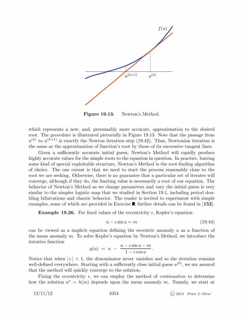
Figure 19.13. Newton’s Method.

which represents a new, and, presumably more accurate, approximation to the desiredroot. The procedure is illustrated pictorially in Figure 19.13. Note that the passage fromu(k) to u(k+1) is exactly the Newton iteration step (19.42). Thus, Newtonian iteration isthe same as the approximation of function’s root by those of its successive tangent lines.

Given a sufficiently accurate initial guess, Newton’s Method will rapidly producehighly accurate values for the simple roots to the equation in question. In practice, barringsome kind of special exploitable structure, Newton’s Method is the root-finding algorithmof choice. The one caveat is that we need to start the process reasonably close to theroot we are seeking. Otherwise, there is no guarantee that a particular set of iterates willconverge, although if they do, the limiting value is necessarily a root of our equation. Thebehavior of Newton’s Method as we change parameters and vary the initial guess is verysimilar to the simpler logistic map that we studied in Section 19.1, including period dou-bling bifurcations and chaotic behavior. The reader is invited to experiment with simpleexamples, some of which are provided in Exercise ; further details can be found in [152].

Example 19.26. For fixed values of the eccentricity ǫ, Kepler’s equation

u− ǫ sinu = m (19.44)

can be viewed as a implicit equation defining the eccentric anomaly u as a function ofthe mean anomaly m. To solve Kepler’s equation by Newton’s Method, we introduce theiterative function

g(u) = u − u− ǫ sinu−m

1− ǫ cosu.

Notice that when | ǫ | < 1, the denominator never vanishes and so the iteration remainswell-defined everywhere. Starting with a sufficiently close initial guess u(0), we are assuredthat the method will quickly converge to the solution.

Fixing the eccentricity ǫ, we can employ the method of continuation to determinehow the solution u⋆ = h(m) depends upon the mean anomaly m. Namely, we start at

12/11/12 1054 c© 2012 Peter J. Olver

0.2 0.4 0.6 0.8 1

0.2

0.4

0.6

0.8

1

1.2

1.4

Figure 19.14. The Solution to the Kepler Equation for Eccentricity ǫ = .5.

m = m0 = 0 with the obvious solution u⋆ = h(0) = 0. Then, to compute the solutionat successive closely spaced values 0 < m1 < m2 < m3 < · · · , we use the previouslycomputed value as an initial guess u(0) = h(mk) for the value of the solution at the nextmesh point mk+1, and run the Newton scheme until it converges to a sufficiently accurateapproximation to the value u⋆ = h(mk+1). As long as mk+1 is reasonably close to mk,Newton’s Method will converge to the solution quite quickly.

The continuation method will quickly produce the values of u at the sample points.Intermediate values can either be determined by an interpolation scheme, e.g., a cubicspline fit of the data, or by running the Newton scheme using the closest known value asan initial condition. A plot for 0 ≤ m ≤ 1 using the value ǫ = .5 appears in Figure 19.14.

Systems of Equations

Let us now turn our attention to nonlinear systems of equations. We shall onlyconsider the case when there are the same number of equations as unknowns:

f1(u1, . . . , un) = 0, . . . fn(u1, . . . , un) = 0. (19.45)

We shall rewrite the system in vector form

f(u) = 0, (19.46)

where f :Rn → Rn is a vector-valued function of n variables. In practice, we do notnecessarily require that f be defined on all of Rn, although this does simplify the exposition.

We shall only consider solutions that are separated from any others. More formally:

Definition 19.27. A solution u⋆ to a system f(u) = 0 is called isolated if thereexists δ > 0 such that f(u) 6= 0 for all u satisfying 0 < ‖u− u⋆ ‖ < δ.

Example 19.28. Consider the planar equation

x2 + y2 = (x2 + y2)2.

12/11/12 1055 c© 2012 Peter J. Olver

Rewriting the equation in polar coordinates as

r = r2 or r(r − 1) = 0,

we immediately see that the solutions consist of the origin x = y = 0 and all points on theunit circle r2 = x2 + y2 = 1. Only the origin is an isolated solution, since every solutionlying on the circle has plenty of other points on the circle that lie arbitrarily close to it.

Typically, solutions to a system of n equations in n unknowns are isolated, althoughthis is not always true. For example, if A is a singular n× n matrix, then the solutions tothe homogeneous linear system Au = 0 form a nontrivial subspace, and so are not isolated.Nonlinear systems with non-isolated solutions can similarly be viewed as exhibiting someform of degeneracy. In general, the numerical computation of non-isolated solutions, e.g.,solving the implicit equations for a curve or surface, is a much more difficult problem, andwe will not attempt to discuss these issues in this introductory presentation. (However, ourcontinuation approach to the Kepler equation in Example 19.26 indicates how one mightproceed in such situations.)

In the case of a single scalar equation, the simple roots, meaning those for whichf ′(u⋆) 6= 0, are the easiest to compute. In higher dimensions, the role of the derivativeof the function is played by the Jacobian matrix (19.28), and this motivates the followingdefinition.

Definition 19.29. A solution u⋆ to a system f(u) = 0 is called nonsingular if theassociated Jacobian matrix is nonsingular there: det f ′(u⋆) 6= 0.

Note that the Jacobian matrix is square if and only if the system has the same numberof equations as unknowns, which is thus one of the requirements for a solution to benonsingular in our sense. Moreover, the Inverse Function Theorem from multivariablecalculus, [9, 129], implies that a nonsingular solution is necessarily isolated.

Theorem 19.30. Every nonsingular solution u⋆ to a system f(u) = 0 is isolated.

Being the multivariate counterparts of simple roots also means that nonsingular solu-tions of systems are the most amenable to practical computation. Computing non-isolatedsolutions, as well as isolated solutions with a singular Jacobian matrix, is a considerablechallenge, and practical algorithms remain much less well developed. For this reason, wefocus exclusively on numerical solution techniques for nonsingular solutions.

Now, let us turn to numerical solution techniques. The first remark is that, unlike thescalar case, proving existence of a solution to a system of equations is often a challengingissue. There is no counterpart to the Intermediate Value Lemma 19.18 for vector-valuedfunctions. It is not hard to find vector-valued functions whose entries take on both positiveand negative values, but admit no solutions; a simple example can be found in Exercise .This precludes any simple analog of the Bisection Method for nonlinear systems in morethan one unknown.

On the other hand, Newton’s Method can be straightforwardly adapted to computenonsingular solutions to systems of equations, and is the most widely used method for this

12/11/12 1056 c© 2012 Peter J. Olver

purpose. The derivation proceeds in very similar manner to the scalar case. First, wereplace the system (19.46) by a fixed point system

u = g(u) (19.47)

having the same solutions. By direct analogy with (19.38), any (reasonable) fixed pointmethod will take the form

g(u) = u− L(u) f(u), (19.48)

where L(u) is an n × n matrix-valued function. Clearly, if f(u) = 0 then g(u) = u;conversely, if g(u) = u, then L(u) f(u) = 0. If we further require that the matrix L(u)be nonsingular, i.e., detL(u) 6= 0, then every fixed point of the iterator (19.48) will be asolution to the system (19.46) and vice versa.

According to Theorem 19.12, the speed of convergence (if any) of the iterative method

u(k+1) = g(u(k)) (19.49)

is governed by the matrix norm (or, more precisely, the spectral radius) of the Jacobianmatrix g′(u⋆) at the fixed point. In particular, if

g′(u⋆) = O (19.50)

is the zero matrix, then the method converges quadratically fast. Let’s figure out how thiscan be arranged. Computing the derivative using the matrix version of the Leibniz rulefor the derivative of a matrix product, (9.40), we find

g′(u⋆) = I − L(u⋆) f ′(u⋆), (19.51)

where I is the n × n identity matrix. (Fortunately, all the terms that involve derivativesof the entries of L(u) go away since f(u⋆) = 0 by assumption; details are relegated toExercise .) Therefore, the quadratic convergence criterion (19.50) holds if and only if

L(u⋆) f ′(u⋆) = I , and hence L(u⋆) = f ′(u⋆)−1

(19.52)

should be the inverse of the Jacobian matrix of f at the solution, which, fortuitously, wasalready assumed to be nonsingular.

As in the scalar case, we don’t know the solution u⋆, but we can arrange that condition(19.52) holds by setting

L(u) = f ′(u)−1

everywhere — or at least everywhere that f has a nonsingular Jacobian matrix. Theresulting fixed point system

u = g(u) = u− f ′(u)−1 f(u), (19.53)

leads to the quadratically convergent Newton iteration scheme

u(k+1) = u(k) − f ′(u(k))−1 f(u(k)). (19.54)

All it requires is that we guess an initial value u(0) that is sufficiently close to the de-sired solution u⋆. We are then guaranteed, by Exercise , that the iterates u(k) convergequadratically fast to u⋆.

12/11/12 1057 c© 2012 Peter J. Olver

Theorem 19.31. Let u⋆ be a nonsingular solution to the system f(u) = 0. Then,

provided u(0) is sufficiently close to u⋆, the Newton iteration scheme (19.54) converges ata quadratic rate to the solution: u(k) → u⋆.

Example 19.32. Consider the pair of simultaneous cubic equations

f1(u, v) = u3 − 3uv2 − 1 = 0, f2(u, v) = 3u2 v − v3 = 0. (19.55)

It is not difficult to prove that there are precisely three solutions:

u⋆1 =

(10

), u⋆

2 =

(−.5

.866025 . . .

), u⋆

3 =

(−.5

−.866025 . . .

). (19.56)

The Newton scheme relies on the Jacobian matrix

f ′(u) =

(3u2 − 3v2 − 6uv

6uv 3u2 − 3v2

).

Since det f ′(u) = 9(u2 + v2) is non-zero except at the origin, all three solutions are non-singular, and hence, for a sufficiently close initial value, Newton’s Method will converge tothe nearby solution. We explicitly compute the inverse Jacobian matrix:

f ′(u)−1 =1

9(u2 + v2)

(3u2 − 3v2 6uv− 6uv 3u2 − 3v2

).

Hence, in this particular example, the Newton iterator (19.53) is

g(u) =

(uv

)− 1

9(u2 + v2)

(3u2 − 3v2 6uv− 6uv 3u2 − 3v2

)(u3 − 3uv2 − 13u2 v − v3

).

A complete diagram of the three basins of attraction, consisting of points whose New-ton iterates converge to each of the three roots, has a remarkably complicated, fractal-likestructure, as illustrated in Figure 19.15. In this plot, the x and y coordinates run from−1.5 to 1.5. The points in the black region all converge to u⋆

1; those in the light gray regionall converge to u⋆

2; while those in the dark gray region all converge to u⋆3. The closer one

is to the root, the sooner the iterates converge. On the interfaces between the basins ofattraction are points for which the Newton iterates fail to converge, but exhibit a random,chaotic behavior. However, round-off errors will cause such iterates to fall into one of thebasins, making it extremely difficult to observe such behavio over the long run.

Remark : The alert reader may notice that in this example, we are in fact merelycomputing the cube roots of unity, i.e., equations (19.55) are the real and imaginary partsof the complex equation z3 = 1 when z = u+ i v.

Example 19.33. A robot arm consists of two rigid rods that are joined end-to-endto a fixed point in the plane, which we take as the origin 0. The arms are free to rotate,and the problem is to configure them so that the robot’s hand ends up at the prescribedposition a = ( a, b )

T. The first rod has length ℓ and makes an angle α with the horizontal,

so its end is at position v1 = ( ℓ cosα, ℓ sinα )T. The second rod has lengthm and makes an

12/11/12 1058 c© 2012 Peter J. Olver

Figure 19.15. Computing the Cube Roots of Unity by Newton’s Method.

α

β

ℓ

m

v1

v1 + v2

Figure 19.16. Robot Arm.

angle β with the horizontal, and so is represented by the vector v2 = (m cosβ,m sinβ )T.

The hand at the end of the second arm is at position v1 + v2, and the problem is to findvalues for the angles α, β so that v1 + v2 = a; see Figure 19.16. To this end, we need tosolve the system of equations

ℓ cosα+m cosβ = a, ℓ sinα +m sinβ = b, (19.57)

for the angles α, β.

To find the solution, we shall apply Newton’s Method. First, we compute the Jacobian

12/11/12 1059 c© 2012 Peter J. Olver

matrix of the system with respect to α, β, which is

f ′(α, β) =

(− ℓ sinα −m sinβℓ cosα m cosβ

),

with inverse

f ′(α, β)−1 =1

ℓm sin(β − α)

(− ℓ sinα m sinβ− ℓ cosα m cosβ

).

As a result, the Newton iteration equation (19.54) has the explicit form(α(k+1)

β(k+1)

)=

(α(k)

β(k)

)−

− 1

ℓm sin(β(k) − α(k))

(− ℓ cosα(k) m sinβ(k)

− ℓ cosα(k) m sinβ(k)

)(ℓ cosα(k) +m cosβ(k) − aℓ sinα(k) +m sinβ(k) − b

).

when running the iteration, one must be careful to avoid points at which α(k) − β(k) = 0or π, i.e., where the robot arm has straightened out.

As an example, let us assume that the rods have lengths ℓ = 2, m = 1, and thedesired location of the hand is at a = ( 1, 1 )

T. We start with an initial guess of α(0) = 0,

β(0) = 12π, so the first rod lies along the x–axis and the second is perpendicular. The first

few Newton iterates are given in the accompanying table. The first column is the iteratenumber k; the second and third columns indicate the angles α(k), β(k) of the rods. Thefourth and fifth give the position (x(k), y(k))T of the joint or elbow, while the final twoindicate the position (z(k), w(k))T of the robot’s hand.

k α(k) β(k) x(k) y(k) z(k) w(k)

0 .0000 1.5708 2.0000 .0000 2.0000 1.0000

1 .0000 2.5708 2.0000 .0000 1.1585 .5403

2 .3533 2.8642 1.8765 .6920 .9147 .9658

3 .2917 2.7084 1.9155 .5751 1.0079 .9948

4 .2987 2.7176 1.9114 .5886 1.0000 1.0000

5 .2987 2.7176 1.9114 .5886 1.0000 1.0000

Observe that the robot has rapidly converged to one of the two possible configurations.(Can you figure out what the second equilibrium is?) In general, convergence depends onthe choice of initial configuration, and the Newton iterates do not always settle down toa fixed point. For instance, if ‖ a ‖ > ℓ +m, there is no possible solution, since the armsare too short for the hand to reach to desired location; thus, no choice of initial conditionswill lead to a convergent scheme and the robot arm flaps around in a chaotic manner.

Now that we have gained a little experience with Newton’s Method for systems ofequations, some supplementary remarks are in order. As we learned back in Chapter 1,except perhaps in very low-dimensional situations, one should not directly invert a matrix,

12/11/12 1060 c© 2012 Peter J. Olver

but rather use Gaussian elimination, or, in favorable situations, a linear iterative scheme,e.g., Jacobi, Gauss–Seidel or even SOR. So a better strategy is to leave the Newton system(19.54) in unsolved, implicit form

f ′(u(k))v(k) = − f(u(k)), u(k+1) = u(k) + v(k). (19.58)

Given the iterate u(k), we compute the Jacobian matrix f ′(u(k)) and the right hand side− f(u(k)), and then use our preferred linear systems solver to find v(k). Adding u(k) tothe result immediately yields the updated approximation u(k+1) to the solution.

The main bottleneck in the implementation of the Newton scheme, particularly forlarge systems, is solving the linear system in (19.58). The coefficient matrix f ′(u(k)) mustbe recomputed at each step of the iteration, and hence knowing the solution to the kth linearsystem does not appear to help us solve the subsequent system. Pereforming a completeGaussian elimination at every step will tend to slow down the algorithm, particularly inhigh dimensional situations involving many equations in many unknowns.

One simple dodge for speeding up the computation is to note that, once we startconverging, u(k) will be very close to u(k−1) and so we will probably not go far wrong byusing f ′(u(k−1)) in place of the updated Jacobian matrix f ′(u(k)). Since we have alreadysolved the linear system with coefficient matrix f ′(u(k−1)), we know its LU factorization,and hence can use Forward and Back Substitution to quickly solve the modified system

f ′(u(k−1))v(k+1) = − f(u(k)), u(k+1) = u(k) + v(k). (19.59)

If u(k+1) is still close to u(k−1), we can continue to use f ′(u(k−1)) as the coefficient matrixwhen proceeding on to the next iterate u(k+2). We proceed in this manner until therehas been a notable change in the iterates, at which stage we can revert to solving thecorrect, unmodified linear system (19.58) by Gaussian Elimination. This strategy maydramatically reduce the total amount of computation required to approximate the solutionto a prescribed accuracy. The down side is that this quasi-Newton scheme is usuallyonly linearly convergent, and so does not home in on the root as fast as the unmodifiedimplementation. The user needs to balance the trade-off between speed of convergenceversus amount of time needed to solve the linear system at each step in the process. See[153] for further discussion.

19.3. Optimization.

We have already noted the importance of quadratic minimization principles for char-acterizing the equilibrium solutions of linear systems of physical significance. In nonlinearsystems, optimization — either maximization or minimization — retains its centrality,and the wealth of practical applications has spawned an entire subdiscipline of appliedmathematics. Physical systems naturally seek to minimize the potential energy function,and so determination of the possible equilibrium configurations requires solving a non-linear minimization principle. Engineering design is guided by a variety of optimizationconstraints, such as performance, longevity, safety, and cost. Non-quadratic minimizationprinciples also arise in the fitting of data by schemes that go beyond the simple linear leastsquares approximation method discussed in Section 4.3. Additional applications naturally

12/11/12 1061 c© 2012 Peter J. Olver

appear in economics and financial mathematics — one often wishes to minimize expensesor maximize profits, in biological and ecological systems, in pattern recognition and signalprocessing, in statistics, and so on. In this section, we will describe the basic mathematicsunderlying simple nonlinear optimization problems along with basic numerical techniques.

The Objective Function

Throughout this section, the real-valued function F (u) = F (u1, . . . , un) to be op-timized — the energy, cost, entropy, performance, etc. — will be called the objective

function. As such, it depends upon one or more variables u = (u1, u2, . . . , un )T

thatbelong to a prescribed subset Ω ⊂ Rn.

Definition 19.34. A point u⋆ ∈ Ω is a global minimum of the objective function

F (u⋆) ≤ F (u) for all u ∈ Ω. (19.60)

The minimum is called strict if

F (u⋆) < F (u) for u⋆ 6= u ∈ Ω. (19.61)

The point u⋆ is called a (strict) local minimum if the relevant inequality holds just forpoints u ∈ Ω nearby u⋆, i.e., satisfying ‖u− u⋆ ‖ < δ for some δ > 0. In particular, strictlocal minima are isolated .

The definition of a maximum — local or global — is the same, but with the reversedinequality: F (u⋆) ≥ F (u) or, in the strict case, F (u⋆) > F (u). Alternatively, a maximumof F (u) is the same as a minimum of the negative −F (u). Therefore, every result thatapplies to minimization of a function can easily be translated into a result on maximization,which allows us to concentrate exclusively on the minimization problem without any loss ofgenerality. We will use extremum as a shorthand term for either a minimum or a maximum.

Remark : As we already noted in Section 4.1, any system of equations can be readilyconverted into a minimization principle. Given a system f(u) = 0, we introduce theobjective function

F (u) = ‖ f(u) ‖2, (19.62)

where ‖ · ‖ is any convenient norm on Rn. By the basic properties of the norm, theminimum value is F (u) = 0, and this is achieved if and only if f(u) = 0, i.e., at a solutionto the system. More generally, if there is no solution to the system, the minimizer(s) ofF (u) play the role of a least squares solution, at least for an inner product-based norm,along with the extensions to more general norms.

In contrast to the rather difficult question of existence of solutions to systems ofequations, there is a general theorem that guarantees the existence of minima (and, hence,maxima) for a broad class of optimization problems.

Theorem 19.35. If F : Ω → R is continuous, and Ω ⊂ Rn is a compact, meaning

closed and bounded, subset, then F has at least one global minimum u⋆ ∈ Ω.

12/11/12 1062 c© 2012 Peter J. Olver

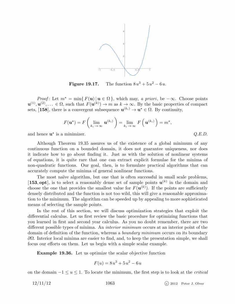
-1 -0.5 0.5 1

2

4

6

Figure 19.17. The function 8u3 + 5u2 − 6u.

Proof : Let m⋆ = minF (u) |u ∈ Ω , which may, a priori , be −∞. Choose pointsu(1),u(2), . . . ∈ Ω, such that F (u(k))→ m as k →∞. By the basic properties of compactsets, [158], there is a convergent subsequence u(ki) → u⋆ ∈ Ω. By continuity,

F (u⋆) = F

(lim

ki →∞u(ki)

)= lim

ki →∞F(u(ki)

)= m⋆,

and hence u⋆ is a minimizer. Q.E.D.

Although Theorem 19.35 assures us of the existence of a global minimum of anycontinuous function on a bounded domain, it does not guarantee uniqueness, nor doesit indicate how to go about finding it. Just as with the solution of nonlinear systemsof equations, it is quite rare that one can extract explicit formulae for the minima ofnon-quadratic functions. Our goal, then, is to formulate practical algorithms that canaccurately compute the minima of general nonlinear functions.

The most naıve algorithm, but one that is often successful in small scale problems,[153, opt], is to select a reasonably dense set of sample points u(k) in the domain andchoose the one that provides the smallest value for F (u(k)). If the points are sufficientlydensely distributed and the function is not too wild, this will give a reasonable approxima-tion to the minimum. The algorithm can be speeded up by appealing to more sophisticatedmeans of selecting the sample points.

In the rest of this section, we will discuss optimization strategies that exploit thedifferential calculus. Let us first review the basic procedure for optimizing functions thatyou learned in first and second year calculus. As you no doubt remember, there are twodifferent possible types of minima. An interior minimum occurs at an interior point of thedomain of definition of the function, whereas a boundary minimum occurs on its boundary∂Ω. Interior local minima are easier to find, and, to keep the presentation simple, we shallfocus our efforts on them. Let us begin with a simple scalar example.

Example 19.36. Let us optimize the scalar objective function

F (u) = 8u3 + 5u2 − 6u

on the domain −1 ≤ u ≤ 1. To locate the minimum, the first step is to look at the critical

12/11/12 1063 c© 2012 Peter J. Olver

points where the derivative vanishes:

F ′(u) = 24u2 + 10u− 6 = 0, and hence u = 13, − 3

4.

To ascertain the local nature of the two critical points, we apply the second derivative test.Since F ′′(u) = 48u+ 10, we have

F ′′ ( 13

)= 26 > 0, whereas F ′′ (− 3

4

)= −26 < 0.

We conclude that 13 is a local minimum, while 3

4 is a local maximum.

To find the global minimum and maximum on the interval [−1, 1], we must also takeinto account the boundary points ±1. Comparing the function values at the four points,

F (−1) = 3, F(13

)= − 31

27≈ −1.148, F

(− 3

4

)= 63

16= 3.9375, F (1) = 7,

we see that 13 is the global minimum, whereas 1 is the global maximum — which occurs on

the boundary of the interval. This is borne out by the graph of the function, as displayedin Figure 19.17.

The Gradient

As you first learn in multi-variable calculus, [9, 129], the interior extrema — minimaand maxima — of a smooth function F (u) = F (u1, . . . , un) are necessarily critical points ,meaning places where the gradient of F vanishes. The standard gradient is the vector fieldwhose entries are its first order partial derivatives:

∇F (u) =

(∂F

∂u1

, . . . ,∂F

∂un

)T

. (19.63)

Let us, in preparation for the more general minimization problems over infinite-dimensionalfunction spaces to be treated in Chapter 21, reformulate the definition of the gradient ina more intrinsic manner. An important but subtle point is that the gradient operator, infact, relies upon the introduction of an inner product on the underlying vector space. Theversion (19.63) is, in fact, based upon on the Euclidean dot product on Rn. Altering theinner product will change the formula for the gradient!

Definition 19.37. Let V be an inner product space. The gradient of a functionF :V → R at a point u ∈ V is the vector ∇F (u) ∈ V that satisfies

〈∇F (u) ;v 〉 = d

dtF (u+ tv)

∣∣∣∣t=0

for all v ∈ V. (19.64)

Remark : The function F does not have to be defined on all of the space V in orderfor this definition to make sense.

The quantity displayed in the preceding formula is known as the directional derivativeof F with respect to v ∈ V , and typically denoted by ∂F/∂v. Thus, by definition, thedirectional derivative equals the inner product with the gradient vector. The directional

12/11/12 1064 c© 2012 Peter J. Olver

derivative measures the rate of change of F in the direction of the vector v, scaled inproportion to its length.

In the Euclidean case, when F (u) = F (u1, . . . , un) is a function of n variables, defined

for u = (u1, u2, . . . , un )T ∈ Rn, we can use the chain rule to compute

d

dtF (u+ tv) =

d

dtF (u1 + t v1, . . . , un + t vn)

=∂F

∂u1

(u+ tv) v1 + · · · + ∂F

∂un

(u+ tv) vn.(19.65)

Setting t = 0, the right hand side of (19.64) reduces to

d

dtF (u+ tv)

∣∣∣∣t=0

=∂F

∂u1

(u) v1 + · · · + ∂F

∂un

(u) vn = ∇F (u) · v.

Therefore, the directional derivative equals the Euclidean dot product between the usualgradient of the function (19.63) and the direction vector v, justifying (19.64) in the Eu-clidean case.

Remark : In this chapter, we will only deal with the standard Euclidean dot product,which results in the usual gradient formula (19.63). If we introduce an alternative innerproduct on Rn, then the notion of gradient, as defined in (19.64) will change. Details areoutlined in Exercise .

A function F (u) is continuously differentiable if and only if its gradient ∇F (u) is acontinuously varying vector-valued function of u. This is equivalent to the requirementthat its first order partial derivatives ∂F/∂ui are all continuous. As usual, we use C1(Ω)to denote the vector space of all continuously differentiable scalar-valued functions definedon a domain Ω ⊂ Rn. From now on, all objective functions are assumed to be continuouslydifferentiable on their domain of definition.

If u(t) represents a parametrized curve contained within the domain of definition ofF (u), then the instantaneous rate of change in the scalar quantity F as we move along thecurve is given by

d

dtF (u(t)) =

⟨∇F (u) ;

du

dt

⟩, (19.66)

which is the directional derivative of F with respect to the velocity or tangent vectorv =

u to the curve. For instance, suppose F (u1, u2) represents the elevation of a mountain

range at position u = (u1, u2 )T. If we travel through the mountains along the path

u(t) = ( u1(t), u2(t) )T, then our instantaneous rate of ascent or descent (19.66) is equal

to the dot product of our velocity vector

u(t) with the gradient of the elevation function.This observation leads to an important interpretation of the gradient vector.

Theorem 19.38. The gradient ∇F (u) of a scalar function F (u) points in the direc-

tion of its steepest increase at the point u. The negative gradient, −∇F (u), which points

in the opposite direction, indicates the direction of steepest decrease.

12/11/12 1065 c© 2012 Peter J. Olver

Thus, when F represents elevation, ∇F tells us the direction that is steepest uphill,while −∇F points directly downhill — the direction water will flow. Similarly, if Frepresents the temperature of a solid body, then ∇F tells us the direction in which itis heating up the quickest. Heat energy (like water) will flow in the opposite, coldestdirection, namely that of the negative gradient vector −∇F .

But you need to be careful in how you interpret Theorem 19.38. Clearly, the fasteryou move along a curve, the faster the function F (u) will vary, and one needs to takethis into account when comparing the rates of change along different curves. The easiestway to effect the comparison is to assume that the tangent vector a =

u has unit norm,so ‖ a ‖ = 1, which means that we are passing through the point u(t) with unit speed.Once this is done, Theorem 19.38 is an immediate consequence of the Cauchy–Schwarzinequality (3.18). Indeed,

∣∣∣∣∂F

∂a

∣∣∣∣ = | a · ∇F | ≤ ‖ a ‖ ‖∇F ‖ = ‖∇F ‖, when ‖ a ‖ = 1,

with equality if and only if a points in the same direction as the gradient. Therefore,the maximum rate of change is when a = ∇F/‖∇F ‖ is the unit vector in the gradientdirection, while the minimum is achieved when a = −∇F/‖∇F ‖ points in the oppositedirection.

Critical Points

Thus, the only points at which the gradient fails to indicate directions of increase/de-crease of the objective fulnction are where it vanishes. Such points play a critical role inthe analysis, whence the following definition.

Definition 19.39. A point u⋆ is called a critical point of the objective function F (u)if

∇F (u⋆) = 0. (19.67)

Let us prove that all local minima are indeed critical points. The most important thingabout this proof is that it only relies on the intrinsic definition of gradient, and thereforeapplies to any function on any inner product space. Moreover, even though the gradientwill change if we alter the underlying inner product, the requirement that it vanish at alocal minimum does not.

Theorem 19.40. Every local (interior) minimum u⋆ of a continuously differentiable

function F (u) is a critical point: ∇F (u⋆) = 0.

Proof : Let 0 6= v ∈ Rn be any vector. Consider the scalar function

g(t) = F (u⋆ + tv) = F (u⋆1 + t v1, . . . , u

⋆n + t vn), (19.68)

where t ∈ R is sufficiently small to ensure that u⋆ + tv remains strictly inside the domainof F . Note that g measures the values of F along a straight line passing through u⋆ in thedirection prescribed by v. Since u⋆ is a local minimum,

F (u⋆) ≤ F (u⋆ + tv), and hence g(0) ≤ g(t)

12/11/12 1066 c© 2012 Peter J. Olver

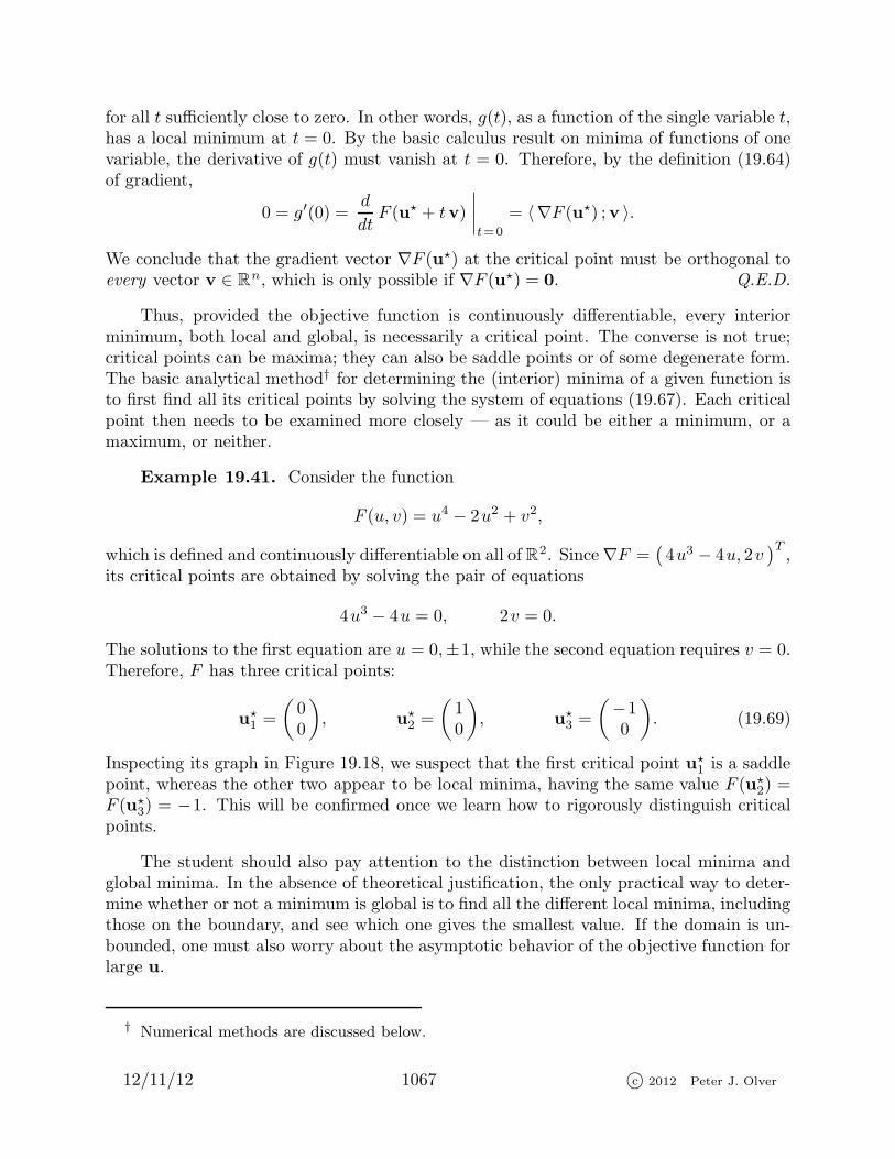
for all t sufficiently close to zero. In other words, g(t), as a function of the single variable t,has a local minimum at t = 0. By the basic calculus result on minima of functions of onevariable, the derivative of g(t) must vanish at t = 0. Therefore, by the definition (19.64)of gradient,

0 = g′(0) =d

dtF (u⋆ + tv)

∣∣∣∣t=0

= 〈∇F (u⋆) ;v 〉.

We conclude that the gradient vector ∇F (u⋆) at the critical point must be orthogonal toevery vector v ∈ Rn, which is only possible if ∇F (u⋆) = 0. Q.E.D.

Thus, provided the objective function is continuously differentiable, every interiorminimum, both local and global, is necessarily a critical point. The converse is not true;critical points can be maxima; they can also be saddle points or of some degenerate form.The basic analytical method† for determining the (interior) minima of a given function isto first find all its critical points by solving the system of equations (19.67). Each criticalpoint then needs to be examined more closely — as it could be either a minimum, or amaximum, or neither.

Example 19.41. Consider the function

F (u, v) = u4 − 2u2 + v2,

which is defined and continuously differentiable on all of R2. Since∇F =(4u3 − 4u, 2v

)T,

its critical points are obtained by solving the pair of equations

4u3 − 4u = 0, 2v = 0.

The solutions to the first equation are u = 0,±1, while the second equation requires v = 0.Therefore, F has three critical points:

u⋆1 =

(00

), u⋆

2 =

(10

), u⋆

3 =

(−10

). (19.69)

Inspecting its graph in Figure 19.18, we suspect that the first critical point u⋆1 is a saddle

point, whereas the other two appear to be local minima, having the same value F (u⋆2) =

F (u⋆3) = −1. This will be confirmed once we learn how to rigorously distinguish critical

points.

The student should also pay attention to the distinction between local minima andglobal minima. In the absence of theoretical justification, the only practical way to deter-mine whether or not a minimum is global is to find all the different local minima, includingthose on the boundary, and see which one gives the smallest value. If the domain is un-bounded, one must also worry about the asymptotic behavior of the objective function forlarge u.

† Numerical methods are discussed below.

12/11/12 1067 c© 2012 Peter J. Olver

Figure 19.18. The Function u4 − 2u2 + v2.

The Second Derivative Test

The status of critical point — minimum, maximum, or neither — can often be resolvedby analyzing the second derivative of the objective function at the critical point. Let usfirst review the one variable second derivative test you learned in first year calculus.

Proposition 19.42. Let g(t) ∈ C2 be a scalar function, and suppose that t⋆ a criticalpoint: g′(t⋆) = 0. If t⋆ is a local minimum, then g′′(t⋆) ≥ 0. Conversely, if g′′(t⋆) > 0,then t⋆ is a strict local minimum. Similarly, g′′(t⋆) ≤ 0 is required at a local maximum,

while g′′(t⋆) < 0 implies that t⋆ is a strict local maximum.

The proof of this result relies on the fact that we can approximate the function by itsquadratic Taylor polynomial near the critical point:

g(t) ≈ g(t⋆) + 12 (t− t⋆)2 g′′(t⋆),

since g′(t⋆) = 0, and so the linear terms in the Taylor polynomial vanish. If g′′(t⋆) 6= 0,then the quadratic Taylor polynomial has a minimum or maximum at t⋆ according to thesign of the second derivative, and this provides the key to the proof. In the borderlinecase, when g′′(t⋆) = 0, the second derivative test is inconclusive, and the point could beeither maximum or minimum or neither. One must analyze the higher order terms in theTaylor expansion to resolve the staus of the critical point; see Exercise .

In multi-variate calculus, the “second derivative” of a function F (u) = F (u1, . . . , un)is represented by the n × n Hessian† matrix , whose entries are its second order partial

† Named after the early eighteenth century German mathematician Ludwig Otto Hesse.

12/11/12 1068 c© 2012 Peter J. Olver

derivatives:

∇2F (u) =

∂2F

∂u21

∂2F

∂u1 ∂u2

. . .∂2F

∂u1 ∂un

∂2F

∂u2 ∂u1

∂2F

∂u22

. . .∂2F

∂u2 ∂un

......

. . ....

∂2F

∂un ∂u1

∂2F

∂un ∂u2

. . .∂2F

∂u2n

, (19.70)

We will always assume that F (u) ∈ C2 has continuous second order partial derivatives. Inthis case, its mixed partial derivatives are equal: ∂2F/∂ui ∂uj = ∂2F/∂uj ∂ui, cf. [9, 129].

As a result, the Hessian is a symmetric matrix: ∇2F (u) = ∇2F (u)T .

The second derivative test for a local minimum of scalar function relies on the positiv-ity of its second derivative. For a function of several variables, the corresponding conditionis that the Hessian matrix be positive definite, as in Definition 3.20. More specifically:

Theorem 19.43. Let F (u) = F (u1, . . . , un) ∈ C2(Ω) be a real-valued, twice con-

tinuously differentiable function defined on an open domain Ω ⊂ Rn. If u⋆ ∈ Ω is a

(local, interior) minimum for F , then it is necessarily a critical point, so ∇F (u⋆) = 0.

Moreover, the Hessian matrix (19.70) must be positive semi-definite at the minimum, so

∇2F (u⋆) ≥ 0. Conversely, if u⋆ is a critical point with positive definite Hessian matrix

∇2F (u⋆) > 0, then u⋆ is a strict local minimum of F .

A maximum requires a negative semi-definite Hessian matrix. If, moreover, the Hes-sian at the critical point is negative definite, then the critical point is a strict local maxi-mum. If the Hessian matrix is indefinite, then the critical point is a saddle point — neitherminimum nor maximum. In the borderline case, when the Hessian is only positive or nega-tive semi-definite at the critical point, the second derivative test is inconclusive. Resolvingthe nature of the critical point requires more detailed knowledge of the objective function,e.g., its higher order derivatives.

We defer the proof of Theorem 19.43 until the end of this section.

Example 19.44. As a first, elementary example, consider the quadratic function

F (u, v) = u2 − 2uv + 3v2.

To minimize F , we begin by computing its gradient

∇F (u, v) =

(2u− 2v−2u+ 6v

).

Solving the pair of equations ∇F = 0, namely

2u− 2v = 0, −2u+ 6v = 0,

12/11/12 1069 c© 2012 Peter J. Olver

we see that the only critical point is the origin u = v = 0. To test whether the origin is amaximum or minimum, we further compute the Hessian matrix

H = ∇2F (u, v) =

(Fuu Fuv

Fuv Fvv

)=

(2 −2−2 6

).

Using the methods of Section 3.5, we easily prove that the Hessian matrix is positivedefinite. Therefore, by Theorem 19.43, u⋆ = 0 is a strict local minimum of F .

Indeed, we recognize F (u, v) to be, in fact, a homogeneous positive definite quadraticform, which can be written in the form

F (u, v) = uTK u, where K =

(1 −1−1 3

)= 1

2H, u =

(uv

).

Positive definiteness of the coefficient matrix K implies that F (u, v) > 0 for all u =

(u, v )T 6= 0, and hence 0 is, in fact, a global minimum.

In general, any quadratic function Q(u) = Q(u1, . . . , un) can be written in the form

Q(u) = uTKu− 2bTu+ c =

m∑

i,j=1

kij uiuj − 2

n∑

i=1

biui + c, (19.71)

where K = KT is a symmetric n × n matrix, b ∈ Rn is a fixed vector, and c ∈ R is ascalar. A straightforward computation produces the formula for its gradient and Hessianmatrix:

∇Q(u) = 2Ku− 2b, ∇2Q(u) = 2K. (19.72)

As a result, the critical points of the quadratic function are the solutions to the linearsystem Ku = b. If K is nonsingular, there is a unique critical point u⋆, which is a strictlocal minimum if and only if K > 0 is positive definite. In fact, Theorem 4.1 tells us that,in the positive definite case, u⋆ is a strict global minimum for Q(u). Thus, the algebraicapproach of Chapter 4 provides additional, global information that cannot be gleaneddirectly from the local, multivariable calculus Theorem 19.43. But algebra is only able tohandle quadratic minimization problems with ease. The analytical classification of minimaand maxima of more complicated objective functions necessarily relies the gradient andHessian criteria of Theorem 19.43.

Example 19.45. The function

F (u, v) = u2 + v2 − v3 has gradient ∇F (u, v) =

(2u

2v − 3v2

).

The critical point equation ∇F = 0 has two solutions: u⋆1 =

(00

)and u⋆

2 =

(023

). The

Hessian matrix of the objective function is

∇2F (u, v) =

(2 00 2− 6v

).

12/11/12 1070 c© 2012 Peter J. Olver

u2 + v2 − v3 u2 + v4 u2 + v3

Figure 19.19. Critical Points.

At the first critical point, the Hessian ∇2F (0, 0) =

(2 00 2

)is positive definite. Therefore,

the origin is a strict local minimum. On the other hand, ∇2F(0, 2

3

)=

(2 00 −2

)is

indefinite, and hence u⋆2 =

(023

)a saddle point. The function is graphed in Figure 19.19,

with the critical points indicated by the small solid balls. The origin is, in fact, only alocal minimum, since F (0, 0) = 0, whereas F (0, v) < 0 for all v > 1. Thus, this particularfunction has no global minimum or maximum on R

2.

Next, consider the function

F (u, v) = u2 + v4, with gradient ∇F (u, v) =

(2u4v3

).

The only critical point is the origin u = v = 0. The origin is a strict global minimumbecause F (u, v) > 0 = F (0, 0) for all (u, v) 6= ( 0, 0 )

T. However, its Hessian matrix

∇2F (u, v) =

(2 00 12v2

)

is only positive semi-definite at the origin, ∇2F (0, 0) =

(2 00 0

).

On the other hand, the origin u = v = 0 is also the only critical point for the function

F (u, v) = u2 + v3 with ∇F (u, v) =

(2u3v2

).

The Hessian matrix is

∇2F (u, v) =

(2 00 6v

), and so ∇2F (0, 0) =

(2 00 0

)

is the same positive semi-definite matrix at the critical point. However, in this case (0, 0)is not a local minimum; indeed

F (0, v) < 0 = F (0, 0) whenever v < 0,

and so there exist points arbitrarily close to the origin where F takes on smaller values.As illustrated in Figure 19.19, the origin is, in fact, a degenerate saddle point.

12/11/12 1071 c© 2012 Peter J. Olver

Finally, the function

F (u, v) = u2 − 2uv + v2 has gradient ∇F (u, v) =

(2u− 2v−2u+ 2v

),

and so every point u = v is a critical point. The Hessian matrix

∇2F (u, v) =

(Fuu Fuv

Fuv Fvv

)=

(2 −2−2 2

)

is positive semi-definite everywhere. Since F (u, u) = 0, while F (u, v) = (u − v)2 > 0when u 6= v, each of these critical points is a non-isolated (and hence non-strict) localminimum. Thus, comparing the three preceding examples, we see that a semi-definiteHessian is unable to distinguish between different types of degenerate critical points.

Finally, the reader should always keep in mind that first and second derivative testsonly determine the local behavior of the function near the critical point. They cannotbe used to determine whether or not we are at a global minimum. This requires someadditional analysis, and, often, a fair amount of ingenuity.

Proof of Theorem 19.43 : We return to the proof of Theorem 19.40. Given a localminimum u⋆, the scalar function g(t) = F (u⋆ + tv) in (19.68) has a local minimum att = 0. As noted above, basic calculus tells us that its derivatives at t = 0 must satisfy

g′(0) = 0, g′′(0) ≥ 0. (19.73)

The first condition leads to the critical point equation ∇F (u⋆) = 0. A straightforwardchain rule calculation produces the formula

g′′(0) =

n∑

i,j=1

∂2F

∂ui ∂uj

(u⋆) vi vj = vT ∇2F (u⋆)v.

As a result, the second condition in (19.73) requires that

vT ∇2F (u⋆)v ≥ 0.

Since this condition is required for every direction v ∈ Rn, the Hessian matrix∇2F (u⋆) ≥ 0satisfies the criterion for positive semi-definiteness, proving the first part of the theorem.

The proof of the converse relies† on the second order Taylor expansion of the function:

F (u) = F (u⋆) +∇F (u⋆) · v + 12 v

T∇2F (u⋆)v + S(v,u⋆)

= F (u⋆) + 12 v

T∇2F (u⋆)v + S(v,u⋆),where v = u− u⋆,

(19.74)

† Actually, it is not hard to prove the first part using the first order Taylor expansion withoutresorting to the scalar function g; see Exercise . On the other hand, when we look at infinite-dimensional minimization problems arising in the calculus of variations, we will no longer have theluxury of appealilng to the finite-dimensional Taylor expansion, whereas the previous argumentcontinues to apply in general contextx.

12/11/12 1072 c© 2012 Peter J. Olver

at the critical point, whence ∇F (u⋆) = 0. The remainder term in the Taylor formula goesto 0 as u→ u⋆ at a rate faster than quadratic:

S(v,u⋆)

‖v ‖2 −→ 0 as v −→ 0. (19.75)

Assuming ∇2F (u⋆), there is a constant C > 0 such that

vT∇2F (u⋆)v ≥ C ‖v ‖2 for all v ∈ Rn.

This is a consequence of the Theorem 3.17 on the equivalence of norms, coupled with thefact that every positive definite matrix defines a norm. By (19.75), we can find δ > 0 suchthat

|S(v,u⋆) | < 12C ‖v ‖2 whenever 0 < ‖v ‖ = ‖u− u⋆ ‖ < δ.

But then the Taylor formula (19.74) implies that, for all u satisfying the preceding in-equality,

0 < 12 v

T∇2F (u⋆)v + S(v,u⋆) = F (u)− F (u⋆),

which implies u⋆ is a strict local minimum of F (u). Q.E.D.

Constrained Optimization and Lagrange Multipliers

In many applications, the function to be minimized is subject to constraints. Forinstance, finding boundary minima requires constraining the minima to the boundary ofthe domain. Another example would be to find the minimum temperature on the surfaceof the earth. Assuming the earth is a perfect sphere of radius R, the temperature functionT (u, v, w) is then to be minimized subject to the constraint u2 + v2 + w2 = R2.

Let us focus on finding the minimum value of an objective function F (u) = F (u, v, w)when its arguments (u, v, w) are constrained to lie on a regular surface S ⊂ R3. Suppose

u⋆ = (u⋆, v⋆, w⋆ )T ∈ S is a (local) minimum for the constrained objective function. Let

u(t) = (u(t), v(t), w(t) )T ⊂ S be any curve contained within the surface that passes

through the minimum, with u(0) = u⋆. Then the scalar function g(t) = F (u(t)) musthave a local minimum at t = 0, and hence, in view of (19.66),

0 = g′(0) =d

dtF (u(t))

∣∣∣∣t=0

= ∇F (u(0)) ·

u(0) = ∇F (u⋆) ·

u(0) . (19.76)

Thus, the gradient of the objective function at the surface minimum must be orthogonalto the tangent vector to the curve. Since the curve was constrained to lies entirely in S, itstangent vector

u(0) is tangent to the surface at the point u⋆. Since every tangent vector tothe surface is tangent to some curve contained in the surface, ∇F (u⋆) must be orthogonalto every tangent vector, and hence point in the normal direction to the surface. Thus, acontrained critical point u⋆ ∈ S of a function on a surface is defined so that

∇F (u⋆) = λn, (19.77)

12/11/12 1073 c© 2012 Peter J. Olver

where n denotes the normal to the surface at the point u⋆. The scalar factor λ is known asthe Lagrange multiplier in honor or Lagrange, one of the pioneers of constrained optimiza-tion. The value of the Lagrange multiplier is not fixed a priori., but must be determinedby solving the critical point system (19.77). The same reasoning applies to local maxima,which are also constrained critical points. The nature of a constrained critical point —local minimum, local maximum, local saddle point, etc. — is fixed by a constrained secondderivative test; details are discussed in Exercise .

Example 19.46. Our problem is to find the minimum value of the objective functionF (u, v, w) = u2−2w3 when u, v, w are restricted to the unit sphere S = (u2 + v2 + w2 = 1).

The radial vector n = (u, v, w )Tis normal to the sphere, and so the critical point condition

(19.77) is

∇F =

2u0

−6w2

= λ

uvw

.

Thus, we must solve the system of equations

2u = λu, 0 = λ v, −6w2 = λw, subject to u2 + v2 + w2 = 1,

for the unknowns u, v, w and λ. This needs to be done carefully to avoid missing any cases.First, if u 6= 0, then λ = 2, v = 0, and either w = 0 whence u = ±1, or w = − 1

3 and so

u = ±√1− w2 = ± 2

√2

3. On the other hand, if u = 0, then either λ = 0, w = 0 and so

v = ±1, or v = 0, w = ±1, and λ = ∓6. Collecting these together, we discover that thereare a total of 8 critical points on the unit sphere:

u⋆1 =

100

, u⋆

2 =

−100

, u⋆

3 =

2√2

3

0

− 13

, u⋆

4 =

− 2

√2

3

0

− 13

,

u⋆5 =

010

, u⋆

6 =

0−10

, u⋆

7 =

001

, u⋆

8 =

00−1

.

Since the unit sphere is closed and bounded, we are assured that F has a global maximumand a global minimum when restricted to S, which are both to be found among ourcandidate critical points. Thus, we merely compute the value of the objective function ateach critical point,

F (u⋆1) = 1, F (u⋆

2) = 1, F (u⋆3) =

2227

, F (u⋆4) =

2627

,

F (u⋆5) = 0, F (u⋆

6) = 0, F (u⋆7) = −2, F (u⋆

8) = 2.

Therefore, u⋆7 must be the global minimum and u⋆

8 the global maximum of the objectivefunction restricted to the unit sphere. The status of the other six critical points — con-strainned local maximum, minimum, or neither — is less evident, and a full classificationrequires the second derivative test outlined in Exercise .

12/11/12 1074 c© 2012 Peter J. Olver

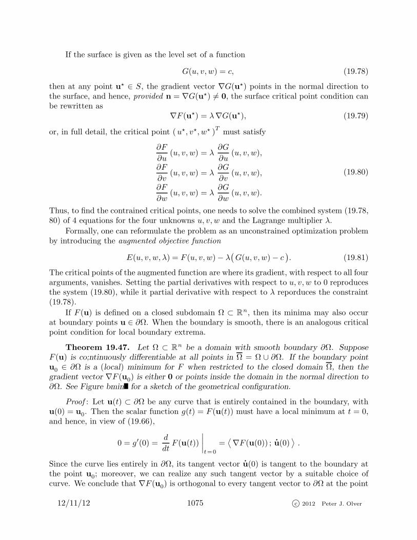
If the surface is given as the level set of a function

G(u, v, w) = c, (19.78)

then at any point u⋆ ∈ S, the gradient vector ∇G(u⋆) points in the normal direction tothe surface, and hence, provided n = ∇G(u⋆) 6= 0, the surface critical point condition canbe rewritten as

∇F (u⋆) = λ∇G(u⋆), (19.79)

or, in full detail, the critical point (u⋆, v⋆, w⋆ )Tmust satisfy

∂F

∂u(u, v, w) = λ

∂G

∂u(u, v, w),

∂F

∂v(u, v, w) = λ

∂G

∂v(u, v, w),

∂F

∂w(u, v, w) = λ

∂G

∂w(u, v, w).

(19.80)

Thus, to find the contrained critical points, one needs to solve the combined system (19.78,80) of 4 equations for the four unknowns u, v, w and the Lagrange multiplier λ.

Formally, one can reformulate the problem as an unconstrained optimization problemby introducing the augmented objective function

E(u, v, w, λ) = F (u, v, w)− λ(G(u, v, w)− c

). (19.81)

The critical points of the augmented function are where its gradient, with respect to all fourarguments, vanishes. Setting the partial derivatives with respect to u, v, w to 0 reproducesthe system (19.80), while it partial derivative with respect to λ reporduces the constraint(19.78).

If F (u) is defined on a closed subdomain Ω ⊂ Rn, then its minima may also occur

at boundary points u ∈ ∂Ω. When the boundary is smooth, there is an analogous criticalpoint condition for local boundary extrema.

Theorem 19.47. Let Ω ⊂ Rn be a domain with smooth boundary ∂Ω. Suppose

F (u) is co;ntinuously differentiable at all points in Ω = Ω ∪ ∂Ω. If the boundary point

u0 ∈ ∂Ω is a (local) minimum for F when restricted to the closed domain Ω, then the

gradient vector ∇F (u0) is either 0 or points inside the domain in the normal direction to

∂Ω. See Figure bmin for a sketch of the geometrical configuration.

Proof : Let u(t) ⊂ ∂Ω be any curve that is entirely contained in the boundary, withu(0) = u0. Then the scalar function g(t) = F (u(t)) must have a local minimum at t = 0,and hence, in view of (19.66),

0 = g′(0) =d

dtF (u(t))

∣∣∣∣t=0

=⟨∇F (u(0)) ;

u(0)⟩.

Since the curve lies entirely in ∂Ω, its tangent vector

u(0) is tangent to the boundary atthe point u0; moreover, we can realize any such tangent vector by a suitable choice ofcurve. We conclude that ∇F (u0) is orthogonal to every tangent vector to ∂Ω at the point

12/11/12 1075 c© 2012 Peter J. Olver

u0, and hence must point in the normal direction to the boundary. Moreover, if non-zero,it cannot point outside Ω since then −∇F (u0), which is the direction of decrease in theobjective function, would point inside the domain, which would preclude u0 from being alocal minimum. Q.E.D.

The same ideas can be applied to optimization problems involving functions of severalvaraibles subject to one or more constraints. Suppose the objective function F (u) =F (u1, . . . , un) is subject to the constraints

G1(u) = c1, · · · Gk(u) = ck. (19.82)

A point u satisfying the constraints is termed regular if the corresponding gradient vectors∇G1(u), . . . ,∇Gk(u) are linearly independent. (Irregular points are more tricky, and mustbe handled separately.) A regular constrained critical point necessarily satisfies the vectorequation

∇F (u) = λ1∇G1(u) + · · · + λ1∇G1(u), (19.83)

where the unspecified scalars λ1, . . . , λk are called the Lagrange multipliers for the con-strained optimization problem. The critical points are thus found by solving the combinedsystem (19.82–83) for the n + k varaibles u1, . . . , un and λ1, . . . , λk. As in (19.81) wecan reformulate this as an uncontrained optimization problem for the augmented objective

function

E(u,λ) = F (u)−k∑

i=1

λi

(Gi(u)− ci

). (19.84)

The gradient with respect to u reproduces the critical point system (19.83), while itsgradient with respect to to λ = (λ1, . . . , λk) recovers the constraints (19.82).

Theorem 19.48. Every regular constrained local minimum and maximum is a con-

strained critical point.

Example 19.49. The problem is to find the point or points on the intersection ofthe elliptical cylinders

u2 + 4v2 = 1, u2 + 9w2 = 4, (19.85)

that is the closest to the origin. Thus, we seek to minimize the squared† distance function

F (u, v, w) = u2 + v2 + w2

subject to the constraints

G(u, v, w) = u2 + 4v2 = 1, H(u, v, w) = u2 + 9w2 = 4,

The augmented objective function (19.81) is

E(u, v, w, λ, µ) = u2 + v2 + w2 − λ(u2 + 4v2 − 1

)+ µ

(u2 + 9w2 − 4

).

† Any distance minimizer also minimizes the squared distance; we work with the latter in orderto avoid square roots in the computation.

12/11/12 1076 c© 2012 Peter J. Olver

To find its critical points, we set all its partial derivatives to zero:

∂E

∂u= 2u+ 2λu+ 2µu = 0,

∂E

∂v= 2v + 8λv = 0,

∂E

∂w= 2w + 18λw = 0,

while the partial derivatives with respect to the Lagrange multipliers λ, µ reproduce thetwo constraints (19.85). Thus,

either u = 0 or λ+ µ = −1, either v = 0 or λ = − 14 , and either w = 0 or µ = − 1

18 .

Thus, at least one of u, v, w must be zero. If u = 0, then v = ± 12 , w = ± 2

3 ; if v = 0,then u = ±1, w = ± 1√

3; while there are no real solutions to the constraints when w = 0.

The first four critical points,(0,± 1

2 ,± 23

)T, all lie a distance 5

6 ≈ .8333 from the origin,

while the second four,(±1, 0,± 2

3

)T, are further away, at distance

√23 ≈ 1.1547. Thus,

the closest points on intersection of the cylinders are the first four, while the furthestpoints from the origin are the last four. (The latter comment relies on the fact that theintersection is a bounded subset of R3.)

Remark : A second derivative test for constrained minima and maxima can be foundin [129].

Numerical Minimization of Scalar Functions

In practical optimization, one typically bypasses the preliminary characterization ofminima as critical points, and instead implements a direct iterative procedure that con-structs a sequence of successively better approximations to the desired minimum. As thecomputation progresses, the approximations are adjusted so that the objective functionis made smaller and smaller, which, we hope, will ensure that we are converging to someform of minimum.

As always, to understand the issues involved, it is essential to consider the simplestscalar situation. Thus, we are given the problem of minimizing a scalar function F (u) ona bounded interval a ≤ u ≤ b. The minimum value can either be at an endpoint or aninterior minimum. Let us first state a result that plays a similar role to the IntermediateValue Lemma 19.18 that formed the basis of the Bisection Method for locating roots.

Lemma 19.50. Suppose that F (u) is defined and continuous for all a ≤ u ≤ b.Suppose that we can find a point a < c < b such that F (c) < F (a) and F (c) < F (b). ThenF (u) has a minimum at some point a < u⋆ < b.

The proof is an easy consequence of Theorem 19.35. Therefore, if we find three pointsa < c < b satisfying the conditions of the lemma, we are assured of the existence of a localminimum for the function between the two endpoints. Once this is done, we can designan algorithm to home in on the minimum u⋆. We choose another point, say d betweena and c and evaluate F (d). If F (d) < F (c), then F (d) < F (a) also, and so the pointsa < d < c satisfy the hypotheses of Lemma 19.50. Otherwise, if F (d) > F (c) then thepoints d < c < b satisfy the hypotheses of the lemma. In either case, a local minimumhas been narrowed down to a smaller interval, either [a, c ] or [d, b ]. In the unlikely even

12/11/12 1077 c© 2012 Peter J. Olver

that F (d) = F (c), one can try another point instead — unless the objective function isconstant, one will eventually find a suitable value of d. Iterating the method will producea sequence of progressively smaller and smaller intervals in which the minimum is trapped,and, just like the Bisection Method, the endpoints of the intervals get closer and closer tou⋆.

The one question is how to choose the point d. We described the algorithm whenit was selected to lie between a and c, but one could equally well try a point betweenc and b. To speed up the algorithm, it makes sense to place d in the larger of the twosubintervals [a, c ] and [c, b ]. One could try placing d in the midpoint of the interval, buta more inspired choice is to place it at a fraction θ = 5√

2− 1

2 ≈ .61803 of the way along

the interval, i.e., at θa + (1 − θ)c if[a, c ] is the longer interval. (One could equally welltake the point (1−θ)a+θ c.) The result is the Golden Section Method . At each stage, thelength of the interval has been reduced by a factor of θ, so the convergence rate is linear,although a bit slower than bisection.

Another strategy is to use an interpolating polynomial passing through the threepoints on the graph of F (u) and use its minimum value as the next approximation to theminimum. According to Exercise 4.4.24, the minimizing value occurs at

d =ms − nt

s− t,

where

s =F (c)− F (a)

c− a, t =

F (b)− F (c)

b− c, m =

a+ c

2, n =

c+ b

2.

As long as a < c < b satisfy the hypothesis of Lemma 19.50, we are assured that thequadratic interpolant has a minimum (and not a maximum!), and that the minimumremains between the endpoints of the interval: a < d < b. If the length of the interval issmall, the minimum value should be a good approximation to the minimizer u⋆ of F (u)itself. Once d is determined, the algorithm proceeds as before. In this case, convergence isnot quite guaranteed, or, in unfavorable situations, could be much slower than the GoldenSection Method. One can even try using the method when the function values do notsatisfy the hypothesis of Lemma 19.50, although now the new point d will not necessarilylie between a and b. Worse, the quadratic interpolant may have a maximum at d, and oneends up going in the wrong direction, which can even happen in the minimizing case dueto the discrepancy between it and the objective function F (u). Thus, this method mustbe handled with care.

A final idea is to focus not on the objective function F (u) but rather its derivativef(u) = F ′(u). The critical points of F are the roots of f(u) = 0, and so one can use oneof the solution methods, e.g., Bisection or Newton’s Method, to find the critical points.Of course, one must then take care that the critical point u⋆ is indeed a minimum, as itcould equally well be a maximum of the original objective function. (It will probably notbe an inflection point, as these do not correspond to simple roots of f(u).) The status ofthe critical point can be checked by looking at the sign of F ′′(u⋆) = f ′(u⋆); indeed, if weuse Newton’s Method we will be computing the derivative at each stage of the algorithm,and can stop looking if the derivative turns out to be of the wrong sign.

12/11/12 1078 c© 2012 Peter J. Olver

Gradient Descent

Now, let us turn our attention to multi-dimensional optimization problems. We areseeking to minimize a (smooth) scalar objective function F (u) = F (u1, . . . , un). Accordingto Theorem 19.38, at any given point u in the domain of definition of F , the negativegradient vector −∇F (u), if nonzero, points in the direction of the steepest decrease inF . Thus, to minimize F , an evident strategy is to “walk downhill”, and, to be efficient,walk downhill as fast as possible, namely in the direction −∇F (u). After walking in thisdirection for a little while, we recompute the gradient, and this tells us the new directionto head downhill. With luck, we will eventually end up at the bottom of the valley, i.e.,at a (local) minimum value of the objective function.

This simple idea forms the basis of the Gradient Descent Method for minimizing theobjective function F (u). In a numerical implementation, we start the iterative procedurewith an initial guess u(0), and let u(k) denote the kth approximation to the minimum u⋆.To compute the next approximation, we set out from u(k) in the direction of the negativegradient, and set

u(k+1) = u(k) − tk∇F (u(k)). (19.86)

for some positive scalar tk > 0. We are free to adjust tk so as to optimize our descentpath, and this is the key to the success of the method.

If ∇F (u(k)) 6= 0, then, at least when tk > 0 is sufficiently small,

F (u(k+1)) < F (u(k)), (19.87)

and so u(k+1) is, presumably, a better approximation to the desired minimum. Clearly, wecannot choose tk too large or we run the risk of overshooting the minimum and reversingthe inequality (19.87). Think of walking downhill in the Swiss Alps. If you walk too farin a straight line, which is what happens as tk increases, then you might very well missthe valley and end up higher than you began — not a good strategy for descending to thebottom! On the other hand, if we choose tk too small, taking very tiny steps, then themethod may end up converging to the minimum much too slowly to be of practical use.

How should we choose an optimal value for the factor tk? Keep in mind that the goalis to minimize F (u). Thus, a good strategy would be to set tk equal to the value of t > 0that minimizes the scalar objective function

g(t) = F(u(k) − t∇F (u(k))

)(19.88)

obtained by restricting F (u) to the ray emanating from u(k) that lies in the negativegradient direction. Physically, this corresponds to setting off in a straight line in thedirection of steepest decrease, and continuing on until we cannot go down any further.Barring luck, we will not have reached the actual bottom of the valley, but must thenreadjust our direction and continue on down the hill in a series of straight line paths.

In practice, one can rarely compute the minimizing value t⋆ of (19.88) exactly. Instead,we employ one of the scalar minimization algorithms presented in the previous subsection.Note that we only need to look for a minimum among positive values of t > 0, since ourchoice of the negative gradient direction assures us that, at least for t sufficiently smalland positive, g(t) < g(0).

12/11/12 1079 c© 2012 Peter J. Olver

A more sophisticated approach is to employ the second order Taylor polynomial toapproximate the function and then use its minimum (assuming such exists) as the nextapproximation to the desired minimizer. Specifically, if u(k) is the current approximationto the minimum, then we approximate

F (u) ≈ c(k) + (u− u(k))Tg(k) + 12 (u− u(k))TH(k)(u− u(k)) (19.89)

near u(k), where

c(k) = F (u(k)), g(k) = ∇F (u(k)), H(k) = ∇2F (u(k)), (19.90)

are, respectively, the function value, the gradient and the Hessian at the current iterate. Ifu⋆ is a stric local minimum, then ∇2F (u⋆) is positive definite, and hence, assuming u(k) isclose, so is H(k) = ∇2F (u(k)). Thus, by Theorem 4.1, the quadratic Taylor approximationhas a unique minimum value u(k+1) which satisfies the linear system

H(k)(u(k+1) − u(k)) = −g(k). (19.91)

The solution serves to define the next approximation u(k+1). While not guaranteed toconverge, the method does perform well in all reasonable situations.

12/11/12 1080 c© 2012 Peter J. Olver