Embed Size (px)
DESCRIPTION
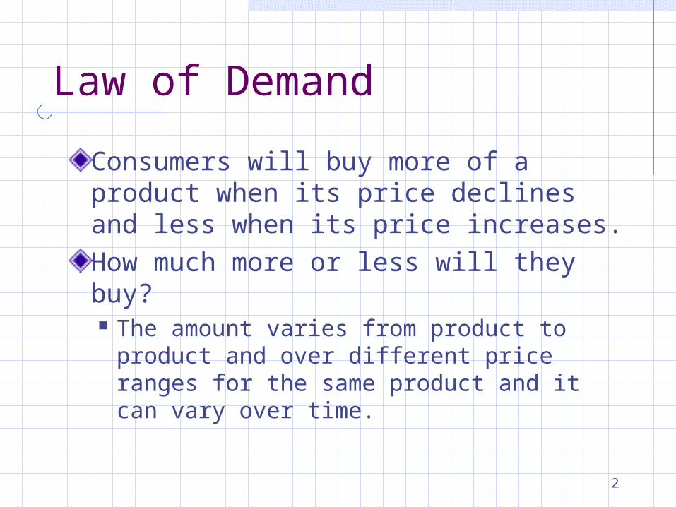
CHAPTER 18 EXTENSIONS OF DEMAND AND SUPPLY. AP ECONOMICS. Law of Demand. Consumers will buy more of a product when its price declines and less when its price increases. How much more or less will they buy? - PowerPoint PPT Presentation
Citation preview

1
CHAPTER 18 EXTENSIONS OF DEMAND AND SUPPLYAP ECONOMICS
2
Law of DemandConsumers will buy more of a product when its price declines and less when its price increases.How much more or less will they buy? The amount varies from product to
product and over different price ranges for the same product and it can vary over time.

3
A BUSINESS CONTEMPLATING A PRICE HIKE, WILL WANT TO KNOW
How will consumers respond Will they remain loyal and thus
increase the revenue of a business Will they “defect en masse” to other
sellers and thus revenue will decrease

4
PRICE ELASTICITY OF DEMAND
Responsiveness of consumers to a price change Examples:
Restaurants Toothpaste
Extent (Degree) to which changes in price cause changes in the quantity demandedTwo types:
Elastic Inelastic
Can help businesses determine pricing policies to increase revenues
5
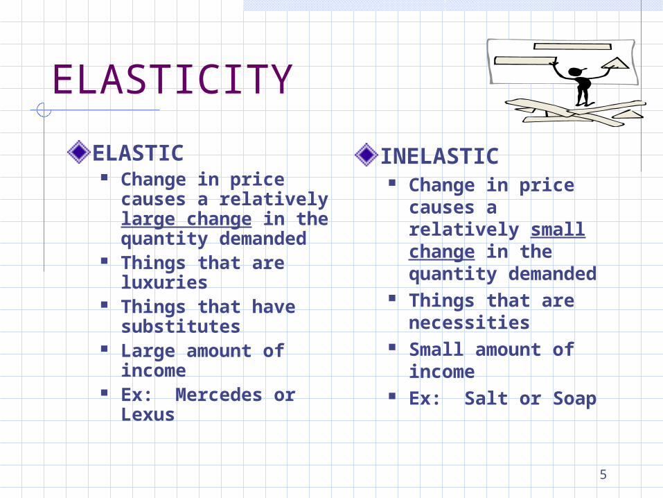
ELASTICITYELASTIC
Change in price causes a relatively large change in the quantity demanded
Things that are luxuries
Things that have substitutes
Large amount of income
Ex: Mercedes or Lexus
INELASTIC Change in price
causes a relatively small change in the quantity demanded
Things that are necessities
Small amount of income
Ex: Salt or Soap

6
Price-Elasticity Coefficient and Formula
Measure degree of price elasticity or inelasticity of demand with Coefficient = Ed
Ed =Percentage Change in Quantity
Demanded of Product XPercentage Change in Price
of Product X

7
Restated Price Elasticy Coefficient
Change in Quantity Demanded of X
Original Price of X
Ed =
Change in Price of XOriginal Quantity Demanded of X
÷

8
Average Midpoint Formula
Change in QuantityEd = Sum of Quantities/2 ÷ Change in PriceSum of Prices/2
9
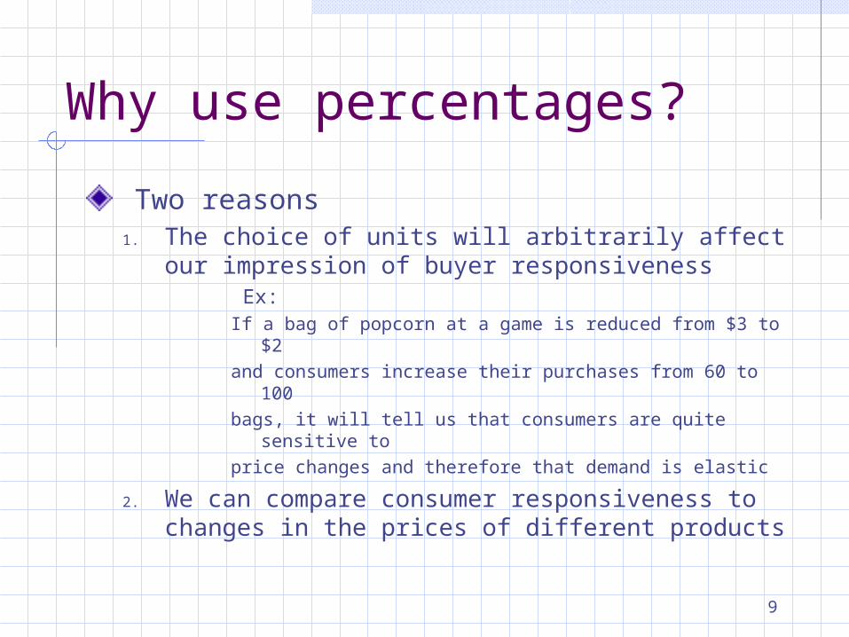
Why use percentages?Two reasons
1. The choice of units will arbitrarily affect our impression of buyer responsiveness Ex:
If a bag of popcorn at a game is reduced from $3 to $2and consumers increase their purchases from 60 to
100bags, it will tell us that consumers are quite sensitive toprice changes and therefore that demand is elastic
2. We can compare consumer responsiveness to changes in the prices of different products
10
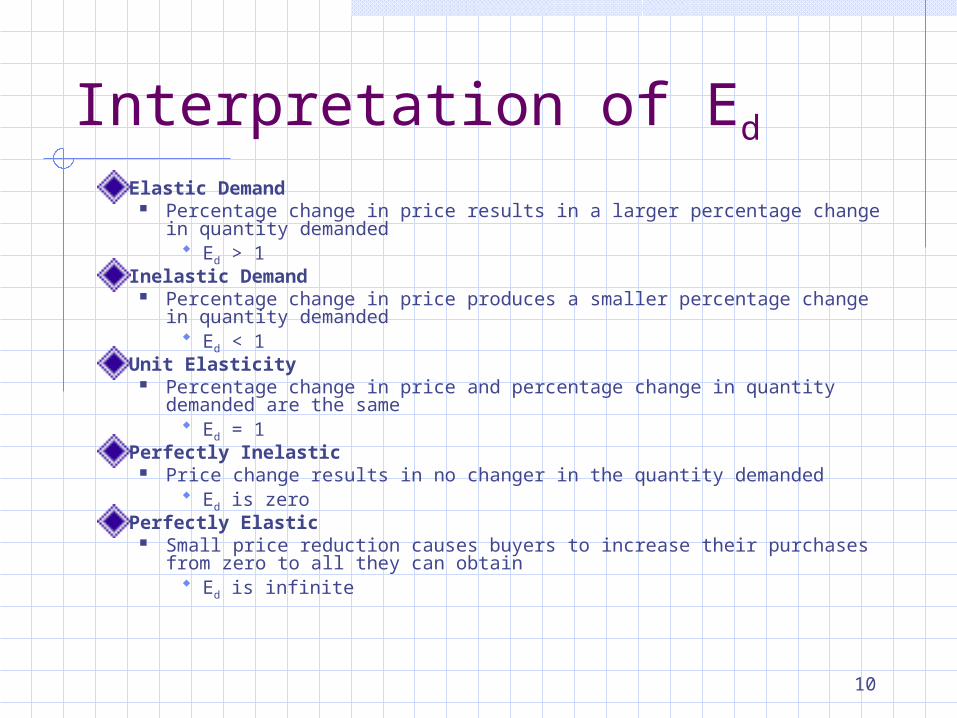
Interpretation of EdElastic Demand
Percentage change in price results in a larger percentage change in quantity demanded
Ed > 1Inelastic Demand
Percentage change in price produces a smaller percentage change in quantity demanded
Ed < 1Unit Elasticity
Percentage change in price and percentage change in quantity demanded are the same
Ed = 1Perfectly Inelastic
Price change results in no changer in the quantity demanded Ed is zero
Perfectly Elastic Small price reduction causes buyers to increase their purchases from zero to
all they can obtain Ed is infinite

11
Price Elasticity of Demand
Extreme CasesPerfectly Inelastic Demand
Perfectly Elastic Demand0
P
Q
P
0 Q
D1
D2
PerfectlyInelasticDemand(Ed = 0)
PerfectlyElasticDemand(Ed = ∞)

12
TOTAL REVENUE TESTTotal revenue is also called total receipts testTo calculate Total Revenue Price X Quantity Sold See Page 344--Chart at bottom of page
Changes in Total Receipts can determine elasticity If TR changes in the opposite direction of the
price, demand is elastic If TR changes in the same direction as price,
demand is inelastic If TR does not change when price changes,
demand is unit-elastic

13
Elastic Demand and TRIf demand is elastic, a decrease in price will increase total revenueIf demand is elastic, a price increase will reduce total revenueSee graph on Page 343 in book

14
Inelastic Demand and TRIf demand is inelastic, a price decrease will reduce total revenueIf demand is inelastic, a price increase will increase total revenueSee graph on Page 343 in book
15
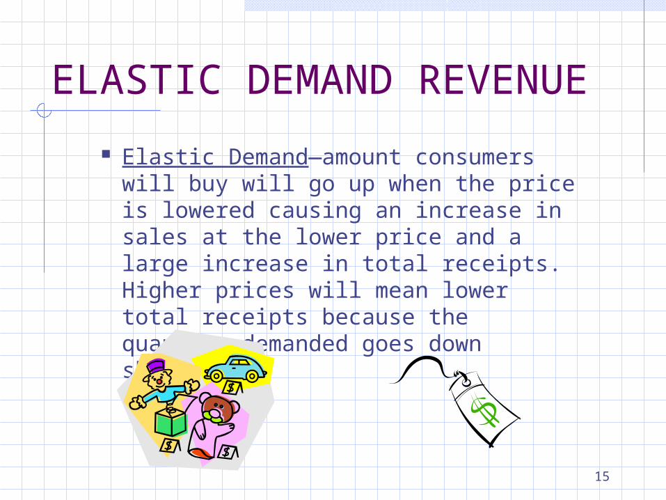
ELASTIC DEMAND REVENUE
Elastic Demand—amount consumers will buy will go up when the price is lowered causing an increase in sales at the lower price and a large increase in total receipts. Higher prices will mean lower total receipts because the quantity demanded goes down sharply.

16
INELASTIC DEMAND REVENUE
Inelastic Demand—lower prices will mean a smaller increase in the quantity demanded and increased sales would not be enough for total receipts to rise. Total revenue will actually increase when prices are raised.

17
DETERMINANTS OF DEMAND ELASTICITY
Can the purchase be delayed? Delayed: elastic Cannot be Delayed: inelasticAre adequate substitutes available? Many substitutes: elastic Few substitutes: inelastic

18
DETERMINANTS CONTINUED
Does the purchase use a large portion of income? Large portion of income: elastic Small portion of income: inelasticSpecific vs. General Market? Gas a particular gas station sells or
gas in general

19
UNIT ELASTIC Unit Elastic--Total revenues neither
increase nor decrease See graph on Page 345 in book
DEMAND SCHEDULEPrice per Pound
Number of Pounds Demanded
Total Receipts
$.80 .70 .60 .50 .40 .30 .20 .10
1,2501,5002,0002,5003,0004,0005,0006,000
$1,000 1,050 1,200 1,250 1,200 1,200 1,000 600
20
Price Elasticity of SupplyIf producers are relatively responsive to price changes, supply is elastic.If producers are relatively insensitive to price changes, supply is inelastic.

21
ELASTICITY OF SUPPLY The degree to which price changes affect the quantity suppliedA product’s supply can be either Elastic Inelastic

22
ELASTIC SUPPLY Exists when a small change in price causes a major change in the quantity supplied Products with elastic supply usually can be made: quickly, inexpensively, and using a few, readily available resourcesSuppliers can change the production rates of such goods easily in order to meet changing consumer demand Examples: Sports teams’ souvenirs, such as
T-shirts, posters, and hats

23
INELASTIC SUPPLY Exists when a change in a good’s price has little impact on the quantity supplied. A product usually has an inelastic supply if production requires a great deal of time, money, and resources that are not readily available.SUPPLIERS cannot easily change the production rates of such goods in order to meet changing consumer demand.
Examples: Gold, fine art, or space shuttles.

24
Measure the Degree of Price Elasticity or Inelasticity
Es
Equation
Percentage Change in QuantitySupplied of Product X
Percentage Change in Priceof Product X
Es =

25
Price Elasticity of SupplyDepends on how easily and therefore quickly producers can shift resources between alternative uses.The longer the time, the greater the resource “shiftability.” The longer a firm has to adjust to a
price change, the greater elasticity of supply

26
Market PeriodPeriod that occurs when the time immediately after a change in market price is too short for producers to respond with a change in quantity suppliedEx. Truckload of tomatoes need a full growing
seasonProducers of goods that can be inexpensively stored, there may be no market period at all.

27
Short RunA period of time too short to change plant capacity, but long enough to use fixed plant more or less intensivelyResult is a somewhat greater output in response to a presumed increase in demand Greater output is reflected in a more elastic
supply of tomatoesEquilibrium price is therefore lower in the short run than in the market period
28
Long RunA time period long enough for firms to adjust their plant sizes and for new firms to enter (or existing firms to leave) the industry.There is not a total revenue test for supplySupply shows a positive or direct relationship between price and amount suppliedSupply curve is upslopingRegardless of the degree of elasticity or inelasticity, price and total revenue always move together

29
Examples of Price Elasticity of Supply
Antiques (inelastic) Reproductions (elastic)Gold (inelastic)
30
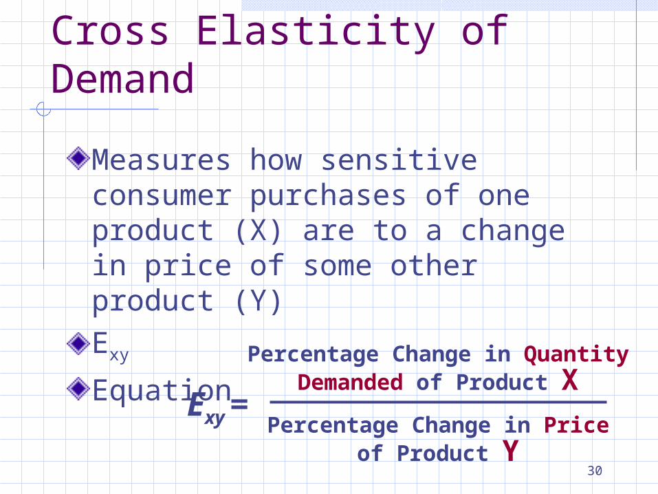
Cross Elasticity of DemandMeasures how sensitive consumer purchases of one product (X) are to a change in price of some other product (Y)Exy
Equation Percentage Change in QuantityDemanded of Product X
Percentage Change in Priceof Product Y
Exy =
31
Cross ElasticityHelps us to more fully understand substitutes and complementary goodsSubstitute Goods
Cross elasticity is positive Sales of X move in the same direction as a change in the price
of Y, then X and Y are substitute goods Ex:
Evian and Dasani The larger the positive cross-elasticity coefficient, the greater is
the substitutability between the two productsComplementary Goods
Cross elasticity is negative X and Y go together Increase in the price of one decreases the demand for the other The larger the negative cross-elasticity coefficient, the greater is
the complementarity between the two goods

32
Independent GoodsA zero or near-zero cross elasticity suggests that the two products being considered are unrelated or independent goods. Ex: walnuts and plums
A change in the price of walnuts does not have an effect on purchases of plums

33
Application of Cross Elasticity
Degree of substitutability of products measured by cross-elasticity co-efficient is important to businesses and governmentUsed to test the sale of one product a company makes against another productGovernments use this for proposed mergers and whether or not they violate anti-trust laws
34
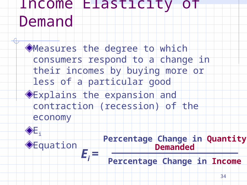
Income Elasticity of Demand
Measures the degree to which consumers respond to a change in their incomes by buying more or less of a particular goodExplains the expansion and contraction (recession) of the economy Ei
Equation Percentage Change in QuantityDemanded
Percentage Change in IncomeEi =

35
Normal Goods versus Inferior Goods
Normal Goods Income elasticity co-efficient is positive More of them are demanded as income rises Also called superior goods Value of Ei varies greatly among normal
goodsInferior Goods Income elasticity co-efficient is negative Less of them are demanded as income rises

36
Cross and Income Elasticity of Demand
Cross Elasticity Positive
Ewz > 0 Quantity demanded of W changes in the same direction as change in price of Z Substitutes
Negative Exy < 0 Quantity demanded of X changes in opposite direction as change in price of Y Complements
Income Elasticity Positive
Ei > 0 Quantity demanded of the product changes in the same direction as change in
income Normal Good
Negative Ei < 0 Quantity demanded of the product changes in opposite direction as change in
income Inferior

37
Consumer SurplusThe difference between maximum price a consumer is willing to pay for a product and actual priceThe utility surplus arises because all consumers pay the equilibrium price even though many would be willing to pay more than that price for the productDemand CurveConsumer surplus and price are inversely related (negative)
Higher prices reduce consumer surplus and lower prices increase consumer surplus

38
Consumer Surplus
Pric
e (P
er B
ag)
P1
Q1
Quantity (Bags)
ConsumerSurplus
Equilibrium Price = $8
D

39
Producer SurplusThe difference between the actual price a producer receives and the minimum acceptable priceSellers receive a producer surplus in most markets because most sellers are willing to accept a lower than equilibrium price in order to sell the productSupply CurveEquilibrium price and amount of producer surplus are directly related (positive)
Lower prices reduce producer surplus and higher prices increase producer surplus

40
Producer Surplus
Pric
e (P
er B
ag)
P1
Quantity (Bags)
ProducerSurplus
Equilibrium Price = $8
S

41
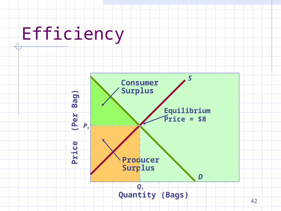
EfficiencyBring supply and demand togetherBring consumer surplus and producer surplus togetherProductive efficiency is achieved because competition forces producers to use the best techniques and combinations of resources in growing and selling productsAllocative efficiency is achieved because the correct quantity of output is produced relative to other goods and services
MB=MC or marginal benefit equals marginal cost Maximum willingness to pay=minimum acceptable price Combined consumer and producer surplus is at a
maximum
42
Efficiency
D
SPr
ice
(Per
Bag
)
P1
Quantity (Bags)
ConsumerSurplus
ProducerSurplus
Equilibrium Price = $8
Q1

43
Efficiency Losses orDeadweight Losses
Reductions of combined consumer and producer surplus associated with underproduction or overproduction of a product

44
Dead Weight Losses
D
SPr
ice
(Per
Bag
)
P1
Q1
Quantity (Bags)
Losses
Q2 Q3
Efficiency