Embed Size (px)
Citation preview
Chapter 17 Probability Models 241
Chapter 17 – Probability Models
1. Bernoulli.
a) These are not Bernoulli trials. The possible outcomes are 1, 2, 3, 4, 5, and 6. There are morethan two possible outcomes.
b) These may be considered Bernoulli trials. There are only two possible outcomes, Type Aand not Type A. Assuming the 120 donors are representative of the population, theprobability of having Type A blood is 43%. The trials are not independent, because thepopulation is finite, but the 120 donors represent less than 10% of all possible donors.
c) These are not Bernoulli trials. The probability of getting a heart changes as cards are dealtwithout replacement.
d) These are not Bernoulli trials. We are sampling without replacement, so the trials are notindependent. Samples without replacement may be considered Bernoulli trials if thesample size is less than 10% of the population, but 500 is more than 10% of 3000.
e) These may be considered Bernoulli trials. There are only two possible outcomes, sealedproperly and not sealed properly. The probability that a package is unsealed is constant, atabout 10%, as long as the packages checked are a representative sample of all packages.Finally, the trials are not independent, since the total number of packages is finite, but the24 packages checked probably represent less than 10% of the packages.
2. Bernoulli 2.
a) These may be considered Bernoulli trials. There are only two possible outcomes, getting a6 and not getting a 6. The probability of getting a 6 is constant at 1/6. The rolls areindependent of one another, since the outcome of one die roll doesn’t affect the other rolls.
b) These are not Bernoulli trials. There are more than two possible outcomes for eye color.
c) These can be considered Bernoulli trials. There are only two possible outcomes, properlyattached buttons and improperly attached buttons. As long as the button problem occursrandomly, the probability of a doll having improperly attached buttons is constant at about3%. The trails are not independent, since the total number of dolls is finite, but 37 dolls isprobably less than 10% of all dolls.
d) These are not Bernoulli trials. The trials are not independent, since the probability ofpicking a council member with a particular political affiliation changes depending on whohas already been picked. The 10% condition is not met, since the sample of size 4 is morethan 10% of the population of 19 people.
e) These may be considered Bernoulli trials. There are only two possible outcomes, cheatingand not cheating. Assuming that cheating patterns in this school are similar to the patternsin the nation, the probability that a student has cheated is constant, at 74%. The trials arenot independent, since the population of all students is finite, but 481 is less than 10% of allstudents.
Copyright 2010 Pearson Education, Inc.
242 Part IV Randomness and Probability
3. Simulating the model.
a) Answers will vary. A component is the simulation of the picture in one box of cereal. Onepossible way to model this component is to generate random digits 0-9. Let 0 and 1represent Tiger Woods and 2-9 a picture of another sports star. Each run will consist ofgenerating random numbers until a 0 or 1 is generated. The response variable will be thenumber of digits generated until the first 0 or 1.
b) Answers will vary.
c) Answers will vary. To construct your simulated probability model, start by calculating thesimulated probability that you get a picture of Tiger Woods in the first box. This is thenumber of trials in which a 0 or 1 was generated first, divided by the total number of trials.Perform similar calculations for the simulated probability that you have to wait until thesecond box, the third box, etc.
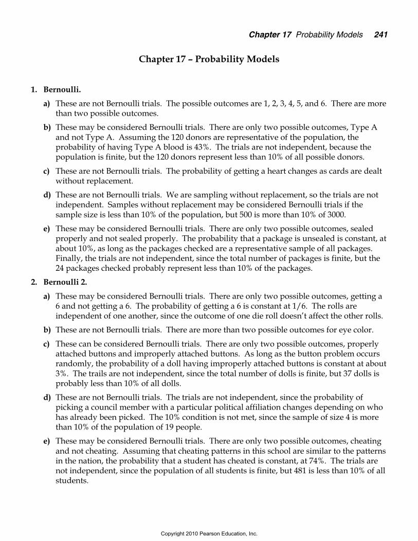
d) Let X = the number of boxes opened until the first Tiger Woods picture is found.
e) Answers will vary.
4. Simulation II.
a) Answers will vary. A component is the simulation of one die roll. One possible way tomodel this component is to generate random digits 1-6. Let 1 represent getting 1 (the rollyou need and let 2-6 represent not getting the roll you need. Each run will consist ofgenerating random numbers until 1 is generated. The response variable will be thenumber of digits generated until the first 1.
b) Answers will vary.
c) Answers will vary. To construct your simulated probability model, start by calculating thesimulated probability that you roll a 1 on the first roll. This is the number of trials in whicha 1 was generated first divided by the total number of trials. Perform similar calculationsfor the simulated probability that you have to wait until the second roll, the third roll, etc.
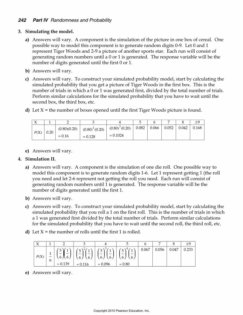
d) Let X = the number of rolls until the first 1 is rolled.
e) Answers will vary.
X 1 2 3 4 5 6 7 8 ≥9
P(X) 0.20( . )( . )
.
0 80 0 20
0 16=( . ) ( . )
.
0 80 0 20
0 128
2
=
( . ) ( . )
.
0 80 0 20
0 1024
3
=
0 082. 0 066. 0 052. 0 042. 0 168.
X 1 2 3 4 5 6 7 8 ≥9
P(X)1
6
5
6
1
6
0 139
≈ .
5
6
1
6
0 116
2
≈ .
5
6
1
6
0 096
3
≈ .
5
6
1
6
0 80
4
≈ .
0 067. 0 056. 0 047. 0 233.
Copyright 2010 Pearson Education, Inc.

Chapter 17 Probability Models 243
5. Tiger again.
a) Answers will vary. A component is the simulation of the picture in one box of cereal. Onepossible way to model this component is to generate random digits 0-9. Let 0 and 1represent Tiger Woods and 2-9 a picture of another sports star. Each run will consist ofgenerating five random numbers. The response variable will be the number of 0s and 1s inthe five random numbers.
b) Answers will vary.
c) Answers will vary. To construct your simulated probability model, start by calculating thesimulated probability that you get no pictures of Tiger Woods in the five boxes. This is thenumber of trials in which neither 0 nor 1 were generated divided by the total number oftrials. Perform similar calculations for the simulated probability that you would get onepicture, 2 pictures, etc.
d) Let X = the number of Tiger Woods pictures in 5 boxes.
e) Answers will vary.
6. Seatbelts.
a) Answers will vary. A component is the simulation of one driver in a car. One possibleway to model this component is to generate pairs of random digits 00-99. Let 01-75represent a driver wearing his or her seatbelt and let 76-99 and 00 represent a driver notwearing his or her seatbelt. Each run will consist of generating five pairs of random digits.The response variable will be the number of pairs of digits that are 00-75.
b) Answers will vary.
c) Answers will vary. To construct your simulated probability model, start by calculating thesimulated probability that none of the five drivers are wearing seatbelts. This is thenumber of trials in which no pairs of digits were 00-75, divided by the total number oftrials. Perform similar calculations for the simulated probability that one driver is wearinghis or her seatbelt, two drivers, etc.
d) Let X = the number of drivers wearing seatbelts in 5 cars.
e) Answers will vary.
X 0 1 2 3 4 5
P(X)
( . ) ( . )
.
0 20 0 80
0 33
0 5
≈
51
1 40 20 0 80
0 41
≈
( . ) ( . )
.
52
2 30 20 0 80
0 20
≈
( . ) ( . )
.
53
3 20 20 0 80
0 05
≈
( . ) ( . )
.
54
4 10 20 0 80
0 01
≈
( . ) ( . )
.
( . ) ( . )
.
0 20 0 80
0 0
5 0
≈
X 0 1 2 3 4 5
P(X)
( . ) ( . )
.
0 75 0 25
0 0
0 5
≈
51
1 40 75 0 25
0 01
≈
( . ) ( . )
.
52
2 30 75 0 25
0 09
≈
( . ) ( . )
.
53
3 20 75 0 25
0 26
≈
( . ) ( . )
.
54
4 10 75 0 25
0 40
≈
( . ) ( . )
.
( . ) ( . )
.
0 75 0 25
0 24
5 0
≈
Copyright 2010 Pearson Education, Inc.
244 Part IV Randomness and Probability
7. On time.
These departures cannot be considered Bernoulli trials. Departures from the same airportduring a 2-hour period may not be independent. They all might be affected by weatherand delays.
8. Lost luggage.
The fate of these bags cannot be considered Bernoulli trials. What happens to 22 pieces ofluggage, all checked on the same flight probably aren’t indpendent.
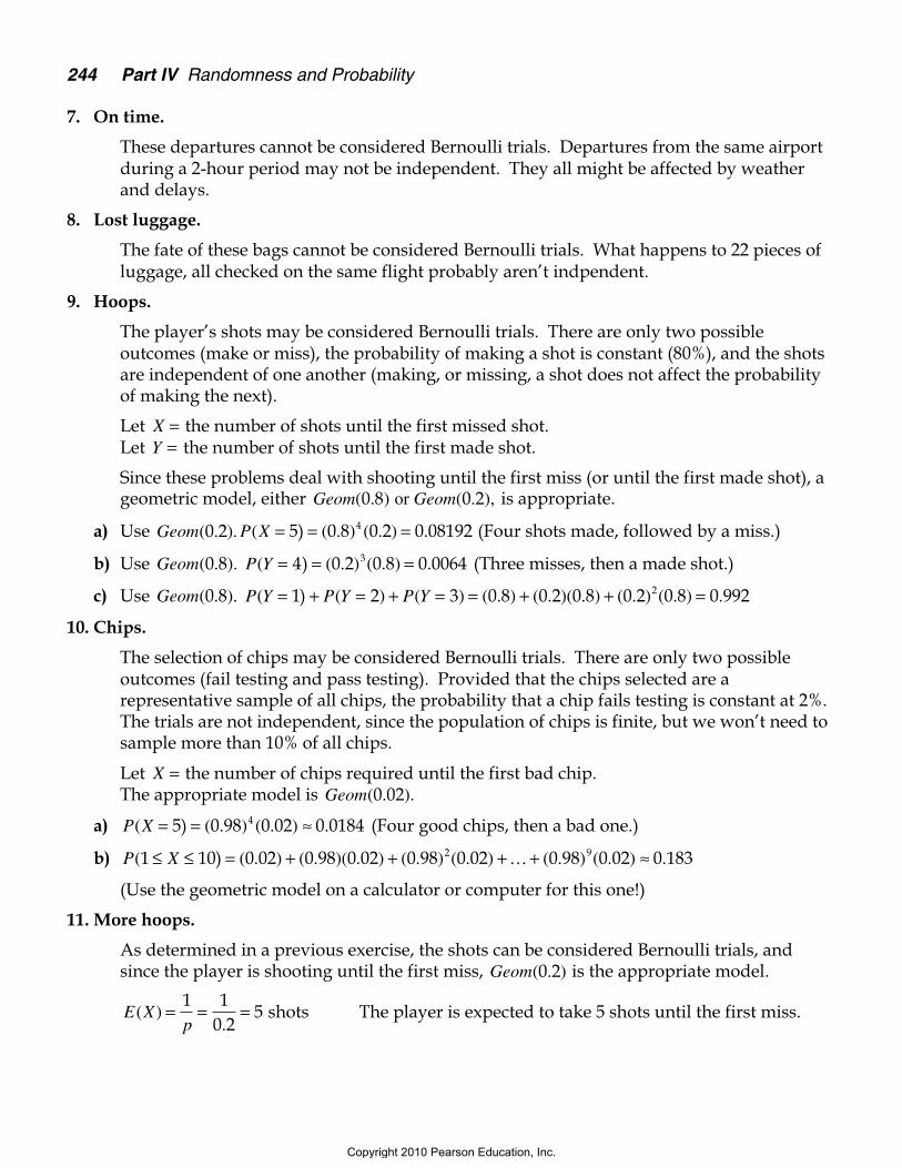
9. Hoops.
The player’s shots may be considered Bernoulli trials. There are only two possibleoutcomes (make or miss), the probability of making a shot is constant (80%), and the shotsare independent of one another (making, or missing, a shot does not affect the probabilityof making the next).
Let X = the number of shots until the first missed shot.Let Y = the number of shots until the first made shot.
Since these problems deal with shooting until the first miss (or until the first made shot), ageometric model, either Geom Geom( . ) ( . ),0 8 0 2 or is appropriate.
a) Use Geom( . ).0 2 P X( ( . ) ( . ) .= = =5 0 8 0 2 0 081924) (Four shots made, followed by a miss.)
b) Use Geom P Y( . ). ( ( . ) ( . ) .0 8 4 0 2 0 8 0 00643 )= = = (Three misses, then a made shot.)
c) Use Geom P Y P Y P Y( . ). ( ( ) ( ) ( . ) ( . )( . ) ( . ) ( . ) .0 8 1 2 3 0 8 0 2 0 8 0 2 0 8 0 9922 )= + = + = = + + =
10. Chips.
The selection of chips may be considered Bernoulli trials. There are only two possibleoutcomes (fail testing and pass testing). Provided that the chips selected are arepresentative sample of all chips, the probability that a chip fails testing is constant at 2%.The trials are not independent, since the population of chips is finite, but we won’t need tosample more than 10% of all chips.
Let X = the number of chips required until the first bad chip.The appropriate model is Geom( . ).0 02
a) P X( ( . ) ( . ) .= = ≈5 0 98 0 02 0 01844) (Four good chips, then a bad one.)
b) P X( ( . ) ( . )( . ) ( . ) ( . ) ( . ) ( . ) .1 10 0 02 0 98 0 02 0 98 0 02 0 98 0 02 0 1832 9≤ ≤ = + + + + ≈) …
(Use the geometric model on a calculator or computer for this one!)
11. More hoops.
As determined in a previous exercise, the shots can be considered Bernoulli trials, andsince the player is shooting until the first miss, Geom( . )0 2 is the appropriate model.
E Xp
( ).
= = =1 1
0 25 shots The player is expected to take 5 shots until the first miss.
Copyright 2010 Pearson Education, Inc.
Chapter 17 Probability Models 245
12. Chips ahoy.
As determined in a previous exercise, the selection of chips can be considered Bernoullitrials, and since the company is selecting until the first bad chip, Geom( . )0 02 is theappropriate model.
E Xp
( ).
= = =1 1
0 0250 chips The first bad chip is expected to be the 50th chip selected.
13. Customer center operator.
The calls can be considered Bernoulli trials. There are only two possible outcomes, takingthe promotion, and not taking the promotion. The probability of success is constant at 5%(50% of the 10% Platinum cardholders.) The trials are not independent, since there are afinite number of cardholders, but this is a major credit card company, so we can assume weare selecting fewer than 10% of all cardholders. Since we are calling people until the firstsuccess, the model Geom( . )0 05 may be used.
Ep
(.
calls) calls.= = =1 1
0 0520 We expect it to take 20 calls to find the first cardholder to take
the double miles promotion.
14. Cold calls.
The donor contacts can be considered Bernoulli trials. There are only two possibleoutcomes, giving $100 or more, and not giving $100 or more. The probability of success isconstant at 1% (5% of the 20% of donors who will make a donation.) The trials are notindependent, since there are a finite number of potential donors, but we will assume thatshe is contacting less than 10% of all possible donors. Since we are contacting people untilthe first success, the model Geom( . )0 01 may be used.
Ep
(.
contacts) contacts.= = =1 1
0 01100 We expect that Justine will have to contact 100
potential donors to find a $100 donor.
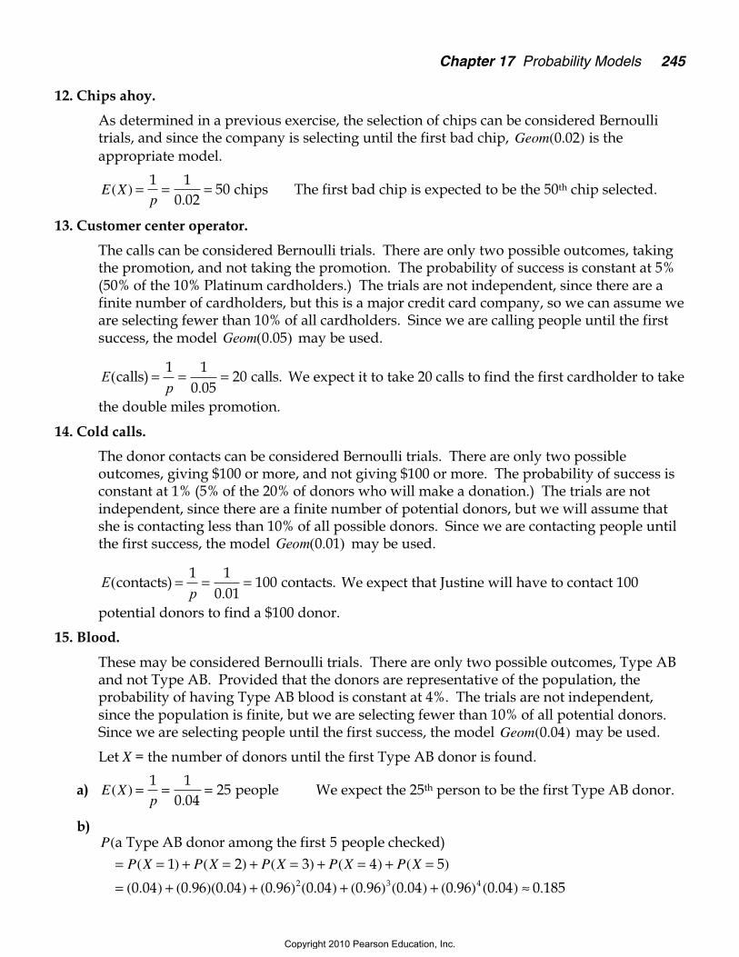
15. Blood.
These may be considered Bernoulli trials. There are only two possible outcomes, Type ABand not Type AB. Provided that the donors are representative of the population, theprobability of having Type AB blood is constant at 4%. The trials are not independent,since the population is finite, but we are selecting fewer than 10% of all potential donors.Since we are selecting people until the first success, the model Geom( . )0 04 may be used.
Let X = the number of donors until the first Type AB donor is found.
a) E Xp
( ).
= = =1 1
0 0425 people We expect the 25th person to be the first Type AB donor.
b)P
P X P X P X P X P X
(
( ) ( ) ( ) ( ) ( )
( . ) ( . )( . ) ( . ) ( . ) ( . ) ( . ) ( . ) ( . ) .
a Type AB donor among the first 5 people checked )
= = + = + = + = + =
= + + + + ≈
1 2 3 4 5
0 04 0 96 0 04 0 96 0 04 0 96 0 04 0 96 0 04 0 1852 3 4
Copyright 2010 Pearson Education, Inc.
246 Part IV Randomness and Probability
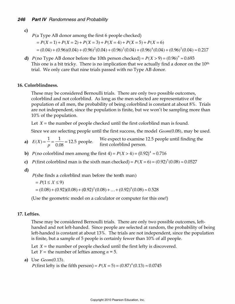
c)P
P X P X P X P X P X P X
(
( ) ( ) ( ) ( ) ( ) ( )
( . ) ( . )( . ) ( . ) ( . ) ( . ) ( . ) ( . ) (
a Type AB donor among the first 6 people checked )
= = + = + = + = + = + =
= + + + +
1 2 3 4 5 6
0 04 0 96 0 04 0 96 0 04 0 96 0 04 0 96 02 3 4 .. ) ( . ) ( . ) .04 0 96 0 04 0 2175+ ≈
d) P P X( ( ) ( . ) .no Type AB donor before the 10th person checked ) = > = ≈9 0 96 0 6939
This one is a bit tricky. There is no implication that we actually find a donor on the 10th
trial. We only care that nine trials passed with no Type AB donor.
16. Colorblindness.
These may be considered Bernoulli trials. There are only two possible outcomes,colorblind and not colorblind. As long as the men selected are representative of thepopulation of all men, the probability of being colorblind is constant at about 8%. Trialsare not independent, since the population is finite, but we won’t be sampling more than10% of the population.
Let X = the number of people checked until the first colorblind man is found.
Since we are selecting people until the first success, the model Geom( . )0 08 , may be used.
a) E Xp
( ).
.= = =1 1
0 0812 5 people.
b) P P X( ( ) .no colorblind men among the first 4 ) (0.92)4= > = ≈4 0 716
c) P P X( ( ) ( . ) ( . ) .first colorblind man is the sixth man checked ) = = = ≈6 0 92 0 08 0 05275
d)P(she finds a colorblind man before the ten tth man )
= ≤ ≤= + +
P X( )
( . ) ( . )( . ) (
1 9
0 08 0 92 0 08 00 92 0 08 0 92 0 08 0 5282 8. ) ( . ) ( . ) ( . ) .+ + ≈…
(Use the geometric model on a calculator or computer for this one!)
17. Lefties.
These may be considered Bernoulli trials. There are only two possible outcomes, left-handed and not left-handed. Since people are selected at random, the probability of beingleft-handed is constant at about 13%. The trials are not independent, since the populationis finite, but a sample of 5 people is certainly fewer than 10% of all people.
Let X = the number of people checked until the first lefty is discovered.Let Y = the number of lefties among n = 5.
a) Use Geom( . )0 13 .P P X( ( ) ( . ) ( . ) .first lefty is the fifth person ) = = = ≈5 0 87 0 13 0 07454
We expect to examine 12.5 people until finding thefirst colorblind person.
Copyright 2010 Pearson Education, Inc.
Chapter 17 Probability Models 247
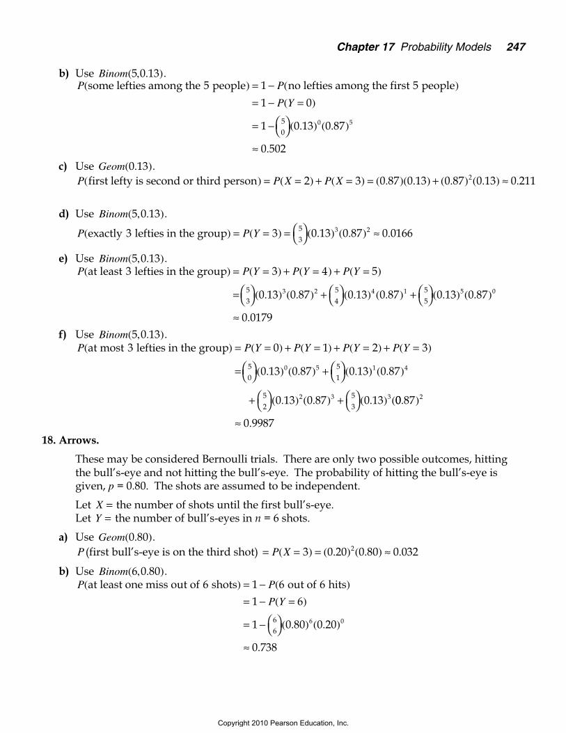
b) Use Binom( , . )5 0 13 .P P
P Y
( (
( )
( . ) ( . )
.
some lefties among the 5 people no lefties among the first 5 people ) )= −= − =
= −
≈
1
1 0
1 0 13 0 87
0 502
50
0 5
c) Use Geom( . )0 13 .P P X P X( ( ) ( ) ( . )( . ) ( . ) ( . ) .first lefty is second or third person ) = = + = = + ≈2 3 0 87 0 13 0 87 0 13 0 2112
d) Use Binom( , . )5 0 13 .
P P Y( ( ) ( . ) ( . ) .exactly 3 lefties in the group ) = = =
≈3 0 13 0 87 0 01665
33 2
e) Use Binom( , . )5 0 13 .P P Y P Y P Y( ( ) ( ) ( )
( . ) ( . ) ( . ) ( . ) ( . ) ( . )
.
at least 3 lefties in the group ) = = + = + =
=
+
+
≈
3 4 5
0 13 0 87 0 13 0 87 0 13 0 87
0 0179
53
54
55
3 2 4 1 5 0
f) Use Binom( , . )5 0 13 .P P Y P Y P Y P Y( ( ) ( ) ( ) ( )
( . ) ( . ) ( . ) ( . )
( . ) ( . ) ( . ) (
at most 3 lefties in the group )
= = + = + = + =
=
+
+
+
0 1 2 3
0 13 0 87 0 13 0 87
0 13 0 87 0 13
50
51
52
53
0 5 1 4
2 3 3 00 87
0 9987
2. )
.≈18. Arrows.
These may be considered Bernoulli trials. There are only two possible outcomes, hittingthe bull’s-eye and not hitting the bull’s-eye. The probability of hitting the bull’s-eye isgiven, p = 0.80. The shots are assumed to be independent.
Let X = the number of shots until the first bull’s-eye.Let Y = the number of bull’s-eyes in n = 6 shots.
a) Use Geom( . )0 80 .P (first bull’s-eye is on the third shot) = = = ≈P X( ) ( . ) ( . ) .3 0 20 0 80 0 0322
b) Use Binom( , . )6 0 80 .P P
P Y
( (
( )
( . ) ( . )
.
at least one miss out of 6 shots 6 out of 6 hits ) )= −= − =
= −
≈
11 6
1 0 80 0 20
0 738
66
6 0
Copyright 2010 Pearson Education, Inc.
248 Part IV Randomness and Probability
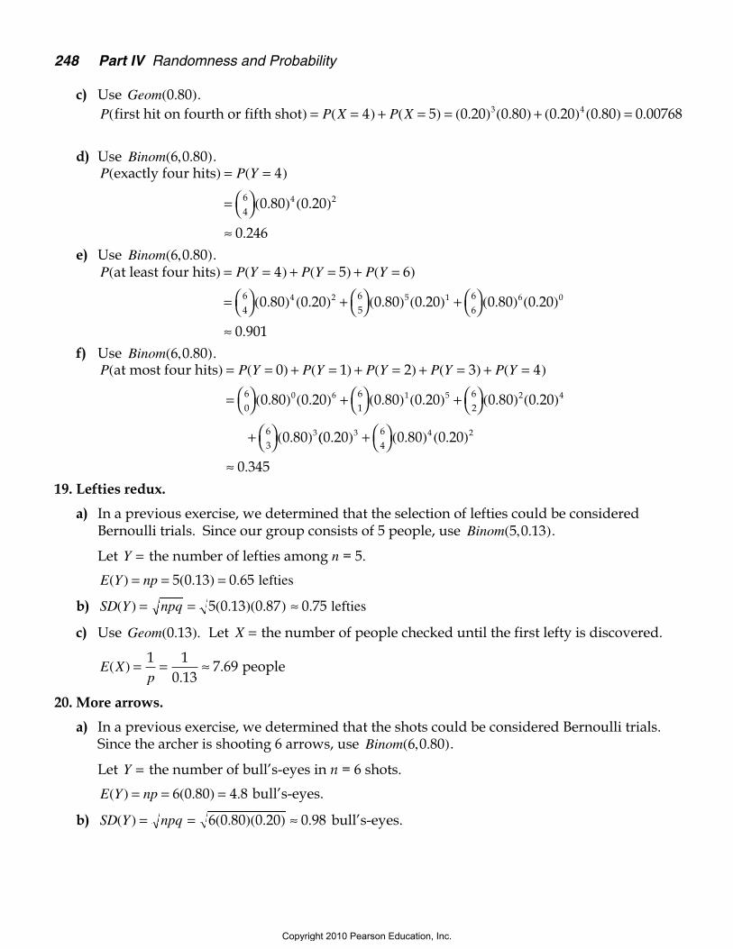
c) Use Geom( . )0 80 .P P X P X( ( ) ( ) ( . ) ( . ) ( . ) ( . ) .first hit on fourth or fifth shot ) = = + = = + =4 5 0 20 0 80 0 20 0 80 0 007683 4
d) Use Binom( , . )6 0 80 .P P Y( )exactly four hits = =
=
≈
( )
( . ) ( . )
.
4
0 80 0 20
0 246
64
4 2
e) Use Binom( , . )6 0 80 .P P Y P Y P Y( )at least four hits = = + = + =
=
+
+
≈
( ) ( ) ( )
( . ) ( . ) ( . ) ( . ) ( . ) ( . )
.
4 5 6
0 80 0 20 0 80 0 20 0 80 0 20
0 901
64
65
66
4 2 5 1 6 0
f) Use Binom( , . )6 0 80 .P P Y P Y P Y P Y P Y( )
at most four hits = = + = + = + = + =
=
+
+
+
( ) ( ) ( ) ( ) ( )
( . ) ( . ) ( . ) ( . ) ( . ) ( . )
( . )
0 1 2 3 4
0 80 0 20 0 80 0 20 0 80 0 20
0 80
60
61
62
63
0 6 1 5 2 4
3(( . ) ( . ) ( . )
.
0 20 0 80 0 20
0 345
3 4 264
+
≈19. Lefties redux.
a) In a previous exercise, we determined that the selection of lefties could be consideredBernoulli trials. Since our group consists of 5 people, use Binom( , . )5 0 13 .
Let Y = the number of lefties among n = 5.
E Y np( ) ( . ) .= = =5 0 13 0 65 lefties
b) SD Y npq( ) ( . )( . ) .= = ≈5 0 13 0 87 0 75 lefties
c) Use Geom( . ).0 13 Let X = the number of people checked until the first lefty is discovered.
E Xp
( ).
.= = ≈1 10 13
7 69 people
20. More arrows.
a) In a previous exercise, we determined that the shots could be considered Bernoulli trials.Since the archer is shooting 6 arrows, use Binom( , . )6 0 80 .
Let Y = the number of bull’s-eyes in n = 6 shots.
E Y np( ) ( . ) .= = =6 0 80 4 8 bull’s-eyes.
b) SD Y npq( ) ( . )( . ) .= = ≈6 0 80 0 20 0 98 bull’s-eyes.
Copyright 2010 Pearson Education, Inc.
Chapter 17 Probability Models 249
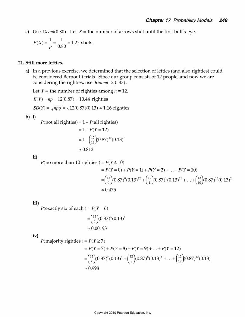
c) Use Geom( . ).0 80 Let X = the number of arrows shot until the first bull’s-eye.
E Xp
( ).
.= = =1 10 80
1 25 shots.
21. Still more lefties.
a) In a previous exercise, we determined that the selection of lefties (and also righties) couldbe considered Bernoulli trials. Since our group consists of 12 people, and now we areconsidering the righties, use Binom( , . )12 0 87 .
Let Y = the number of righties among n = 12.
E Y np( ) ( . ) .= = =12 0 87 10 44 righties
SD Y npq( ) ( . )( . ) .= = ≈12 0 87 0 13 1 16 righties
b) i)P P
P Y
( (
( )
( . ) ( . )
.
not all righties all righties ) )= −= − =
= −
≈
1
1 12
1 0 87 0 13
0 812
1212
12 0
ii)P P Y
P Y P Y P Y P Y
( ( )
( ) ( ) ( ) ( )
( . ) ( . ) ( . ) ( . ) ( . ) ( . )
.
no more than 10 righties ) = ≤= = + = + = + + =
=
+
+ +
≈
10
0 1 2 10
0 87 0 13 0 87 0 13 0 87 0 13
0 475
120
121
1210
0 12 1 11 10 2
…
…
iii)P P Y( ( )
( . ) ( . )
.
exactly six of each ) = =
=
≈
6
0 87 0 13
0 00193
126
6 6
iv)P P Y
P Y P Y P Y P Y
( ( )
( ) ( ) ( ) ( )
( . ) ( . ) ( . ) ( . ) ( . ) ( . )
.
majority righties ) = ≥= = + = + = + + =
=
+
+ +
≈
7
7 8 9 12
0 87 0 13 0 87 0 13 0 87 0 13
0 998
127
128
1212
7 5 8 4 12 0
…
…
Copyright 2010 Pearson Education, Inc.
250 Part IV Randomness and Probability
22. Still more arrows.
a) In a previous exercise, we determined that the archer’s shots could be considered Bernoullitrials. Since our archer is now shooting 10 arrows, use Binom( , . )10 0 80 .
Let Y = the number of bull’s-eyes hit from n = 10 shots.E Y np( ) ( . )= = =10 0 80 8 bull’s-eyes hit.SD Y npq( ) ( . )( . ) .= = ≈10 0 80 0 20 1 26 bull’s-eyes hit.
b) i)P P
P Y
( (
( )
( . ) ( . )
.
no misses out of 10 shots all hits out of 10 shots ) )== =
=
≈
10
0 80 0 20
0 107
1010
10 0
ii)P P Y
P Y P Y P Y P Y
( ( )
( ) ( ) ( ) ( )
( . ) ( . ) ( . ) ( . ) ( . ) ( . )
.
no more than 8 hits ) = ≤= = + = + = + + =
=
+
+ +
≈
80 1 2 8
0 80 0 20 0 80 0 20 0 80 0 20
0 624
100
101
108
0 10 1 9 8 2
…
…
iii)P P Y( ( )
( . ) ( . )
.
exactly 8 out of 10 shots ) = =
=
≈
8
0 80 0 20
0 302
108
8 2
iv)P P Y
P Y P Y P Y
( ( )
( ) ( ) ( )
( . ) ( . ) ( . ) ( . ) ( . ) ( . )
.
more hits than misses ) = ≥= = + = + + =
=
+
+ +
≈
66 7 10
0 80 0 20 0 80 0 20 0 80 0 20
0 967
106
107
1010
6 4 7 3 10 0
…
…
23. Vision.
The vision tests can be considered Bernoulli trials. There are only two possible outcomes,nearsighted or not. The probability of any child being nearsighted is given asp = 0.12. Finally, since the population of children is finite, the trials are not independent.However, 169 is certainly less than 10% of all children, and we will assume that thechildren in this district are representative of all children in relation to nearsightedness.Use Binom( , . ).169 0 12
µ = = = =E np( ( . ) .nearsighted) childre169 0 12 20 28 nn.
σ = = = ≈SD npq( ( . )( . ) .nearsighted) 169 0 12 0 88 4 22 cchildren.
Copyright 2010 Pearson Education, Inc.
Chapter 17 Probability Models 251
24. International students.
The students can be considered Bernoulli trials. There are only two possible outcomes,international or not. The probability of any freshmen being an international student isgiven as p = 0.06. Finally, since the population of freshmen is finite, the trials are notindependent. However, 40 is likely to be less than 10% of all students, and we are told thatthe freshmen in this college are randomly assigned to housing.Use Binom( , . ).40 0 06
µ = = = =E np( ( . ) .international) students40 0 06 2 4 ..
σ = = = ≈SD npq( ( . )( . ) .nearsighted) st40 0 06 0 94 1 5 uudents.
25. Tennis, anyone?
The first serves can be considered Bernoulli trials. There are only two possible outcomes,successful and unsuccessful. The probability of any first serve being good is given asp = 0.70. Finally, we are assuming that each serve is independent of the others. Since she isserving 6 times, use Binom( , . ).6 0 70
Let X = the number of successful serves in n = 6 first serves.
a) b)P P X( ( )
( . ) ( . )
.
all six serves in ) = =
=
≈
6
0 70 0 30
0 118
66
6 0
P P X( ( )
( . ) ( . )
.
exactly four serves in ) = =
=
≈
4
0 70 0 30
0 324
64
4 2
c)P P X P X P X( )at least four serves in = = + = + =
=
+
+
≈
( ) ( ) ( )
( . ) ( . ) ( . ) ( . ) ( . ) ( . )
.
4 5 6
0 70 0 30 0 70 0 30 0 70 0 30
0 744
64
65
66
4 2 5 1 6 0
d)P P X P X P X P X P X( )
no more than four serves in = = + = + = + = + =
=
+
+
+
( ) ( ) ( ) ( ) ( )
( . ) ( . ) ( . ) ( . ) ( . ) ( . )
(
0 1 2 3 4
0 70 0 30 0 70 0 30 0 70 0 30
0
60
61
62
63
0 6 1 5 2 4
.. ) ( . ) ( . ) ( . )
.
70 0 30 0 70 0 30
0 580
3 3 4 264
+
≈26. Frogs.
The frog examinations can be considered Bernoulli trials. There are only two possibleoutcomes, having the trait and not having the trait. If the frequency of the trait has notchanged, and the biologist collects a representative sample of frogs, then the probability ofa frog having the trait is constant, at p = 0.125. The trials are not independent since thepopulation of frogs is finite, but 12 frogs is fewer than 10% of all frogs. Since the biologistis collecting 12 frogs, use Binom( , . ).12 0 125
Let X = the number of frogs with the trait, from n = 12 frogs.
Copyright 2010 Pearson Education, Inc.
252 Part IV Randomness and Probability
a)P P X( ( )
( . ) ( . )
.
no frogs have the trait ) = =
=
≈
0
0 125 0 875
0 201
120
0 12
b)P P X
P X P X P X
( ( )
( ) ( ) ( )
( . ) ( . ) ( . ) ( . ) ( . ) ( . )
.
at least two frogs ) = ≥= = + = + + =
=
+
+ +
≈
2
2 3 12
0 125 0 875 0 125 0 875 0 125 0 875
0 453
12
2
123
1212
2 10 3 9 12 0
…
…
c)P P X P X( ( ) ( )
( . ) ( . ) ( . ) ( . )
.
three or four frogs have trait ) = = + =
=
+
≈
3 4
0 125 0 875 0 125 0 875
0 171
123
124
3 9 4 8
d)P P X P X P X P X( ( ) ( ) ( ) ( )
( . ) ( . ) ( . ) ( . ) ( . ) ( . )
.
no more than four ) = ≤ = = + = + + =
=
+
+ +
≈
4 0 1 4
0 125 0 875 0 125 0 875 0 125 0 875
0 989
120
121
124
0 12 1 11 4 8
…
…
27. And more tennis.
The first serves can be considered Bernoulli trials. There are only two possible outcomes,successful and unsuccessful. The probability of any first serve being good is given asp = 0.70. Finally, we are assuming that each serve is independent of the others. Since she isserving 80 times, use Binom( , . ).80 0 70
Let X = the number of successful serves in n = 80 first serves.
a) E X np( ) ( . )= = =80 0 70 56 first serves in.
SD X npq( ) ( . )( . ) .= = ≈80 0 70 0 30 4 10 first serves in.
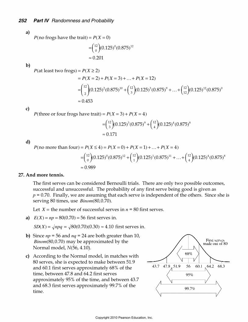
b) Since np = 56 and nq = 24 are both greater than 10,Binom( , . )80 0 70 may be approximated by theNormal model, N(56, 4.10).
c) According to the Normal model, in matches with80 serves, she is expected to make between 51.9and 60.1 first serves approximately 68% of thetime, between 47.8 and 64.2 first servesapproximately 95% of the time, and between 43.7and 68.3 first serves approximately 99.7% of thetime.
Copyright 2010 Pearson Education, Inc.
Chapter 17 Probability Models 253
d) Using Binom(80, 0.70):P P X
P X P X P X
( ( )
( ) ( ) ( )
( . ) ( . ) ( . ) ( . ) ( . ) ( . )
.
at least 65 first serves ) = ≥= = + = + + =
=
+
+ +
≈
6565 66 80
0 70 0 30 0 70 0 30 0 70 0 30
0 0161
8065
8066
8080
65 15 66 14 80 0
…
…
According to the Binomial model, the probability that she makes at least 65 first serves outof 80 is approximately 0.0161.
Using N(56, 4.10):
P X P z( ) ( . ) .≥ ≈ > ≈65 2 195 0 0141
28. More arrows.
These may be considered Bernoulli trials. There are only two possible outcomes, hittingthe bull’s-eye and not hitting the bull’s-eye. The probability of hitting the bull’s-eye isgiven, p = 0.80. The shots are assumed to be independent. Since she will be shooting 200arrows, use Binom(200, 0.80).
Let Y = the number of bull’s-eyes in n = 200 shots.
a) E Y np( ) ( . )= = =200 0 80 160 bull’s-eyes.SD Y npq( ) ( . )( . ) .= = ≈200 0 80 0 20 5 66 bull’s-eyes.
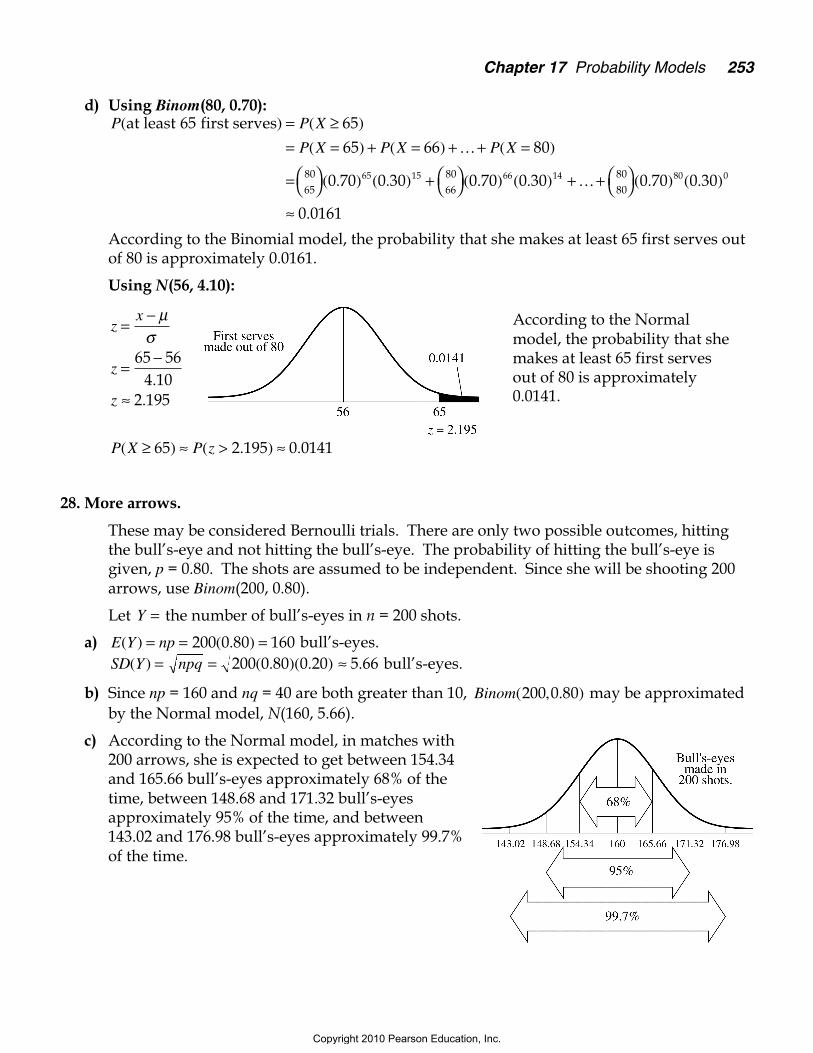
b) Since np = 160 and nq = 40 are both greater than 10, Binom( , . )200 0 80 may be approximatedby the Normal model, N(160, 5.66).
c) According to the Normal model, in matches with200 arrows, she is expected to get between 154.34and 165.66 bull’s-eyes approximately 68% of thetime, between 148.68 and 171.32 bull’s-eyesapproximately 95% of the time, and between143.02 and 176.98 bull’s-eyes approximately 99.7%of the time.
zx
z
z
=−
=−
≈
µσ
65 564 10
2 195.
.
According to the Normalmodel, the probability that shemakes at least 65 first servesout of 80 is approximately0.0141.
Copyright 2010 Pearson Education, Inc.
254 Part IV Randomness and Probability
d) Using Binom(200, 0.80):
P P Y
P Y P Y P Y
( ( )
( ) ( ) ( )
( . ) ( . ) ( . ) ( . ) ( . ) ( . )
.
at most 140 hits ) = ≤= = + = + + =
=
+
+ +
≈
1400 1 140
0 80 0 20 0 80 0 20 0 80 0 70
0 0005
2000
2001
200140
0 200 1 199 140 60
…
…
According to the Binomial model, the probability that she makes at most 140 bull’s-eyesout of 200 is approximately 0.0005.
Using N(160, 5.66):
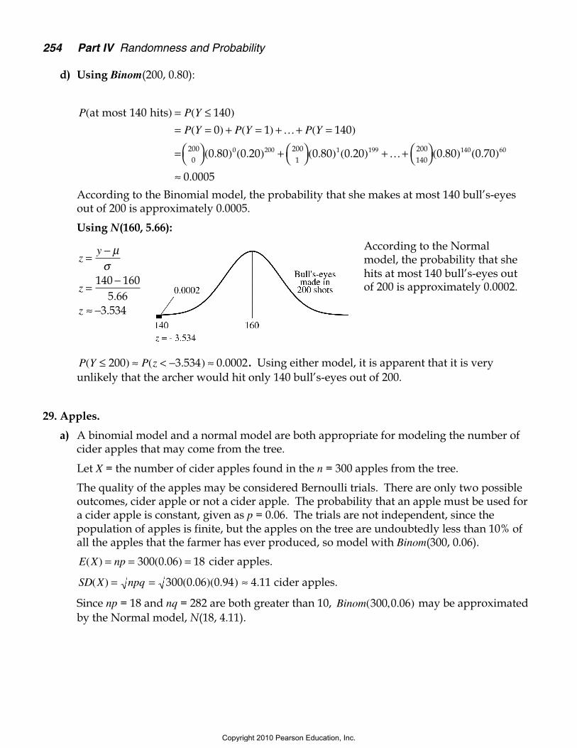
P Y P z( ) ( . ) .≤ ≈ < − ≈200 3 534 0 0002 . Using either model, it is apparent that it is veryunlikely that the archer would hit only 140 bull’s-eyes out of 200.
29. Apples.
a) A binomial model and a normal model are both appropriate for modeling the number ofcider apples that may come from the tree.
Let X = the number of cider apples found in the n = 300 apples from the tree.
The quality of the apples may be considered Bernoulli trials. There are only two possibleoutcomes, cider apple or not a cider apple. The probability that an apple must be used fora cider apple is constant, given as p = 0.06. The trials are not independent, since thepopulation of apples is finite, but the apples on the tree are undoubtedly less than 10% ofall the apples that the farmer has ever produced, so model with Binom(300, 0.06).
E X np( ) ( . )= = =300 0 06 18 cider apples.
SD X npq( ) ( . )( . ) .= = ≈300 0 06 0 94 4 11 cider apples.
Since np = 18 and nq = 282 are both greater than 10, Binom( , . )300 0 06 may be approximatedby the Normal model, N(18, 4.11).
According to the Normalmodel, the probability that shehits at most 140 bull’s-eyes outof 200 is approximately 0.0002.
zy
z
z
=−
=−
≈ −
µσ
140 1605 66
3 534.
.
Copyright 2010 Pearson Education, Inc.
Chapter 17 Probability Models 255
b) Using Binom(300, 0.06):
P P X
P X P X
( ( )
( ) ( )
( . ) ( . ) ( . ) ( . )
.
at most 12 cider apples ) = ≤= = + + =
=
+ +
≈
12
0 12
0 06 0 94 0 06 0 94
0 085
3000
30012
0 300 12 282
…
…
According to the Binomial model, the probability that no more than 12 cider apples comefrom the tree is approximately 0.085.
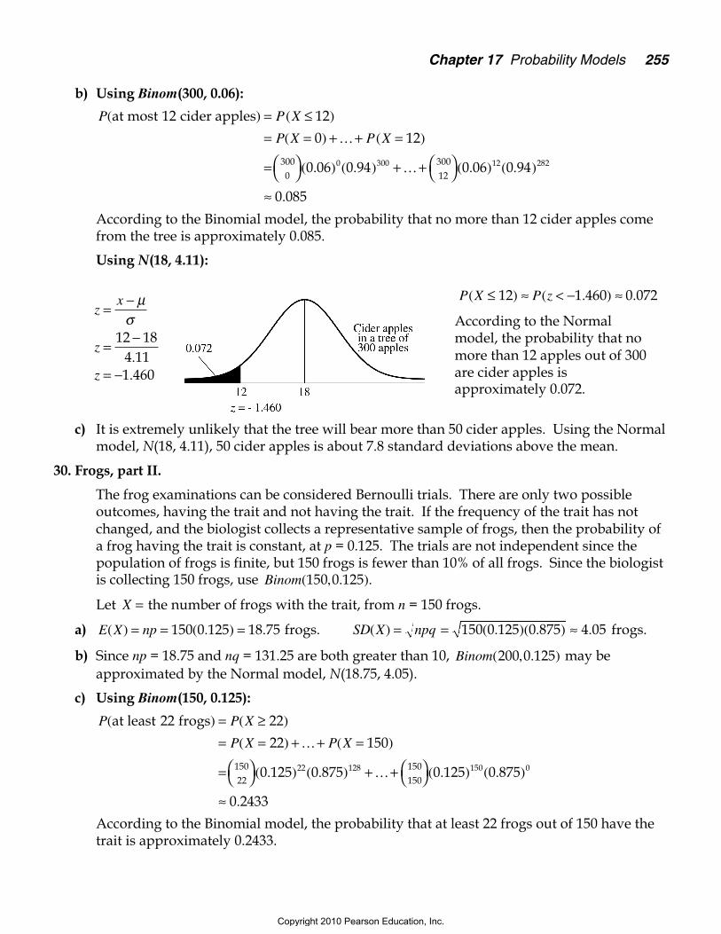
Using N(18, 4.11):
c) It is extremely unlikely that the tree will bear more than 50 cider apples. Using the Normalmodel, N(18, 4.11), 50 cider apples is about 7.8 standard deviations above the mean.
30. Frogs, part II.
The frog examinations can be considered Bernoulli trials. There are only two possibleoutcomes, having the trait and not having the trait. If the frequency of the trait has notchanged, and the biologist collects a representative sample of frogs, then the probability ofa frog having the trait is constant, at p = 0.125. The trials are not independent since thepopulation of frogs is finite, but 150 frogs is fewer than 10% of all frogs. Since the biologistis collecting 150 frogs, use Binom( , . ).150 0 125
Let X = the number of frogs with the trait, from n = 150 frogs.
a) E X np( ) ( . ) .= = =150 0 125 18 75 frogs. SD X npq( ) ( . )( . ) .= = ≈150 0 125 0 875 4 05 frogs.
b) Since np = 18.75 and nq = 131.25 are both greater than 10, Binom( , . )200 0 125 may beapproximated by the Normal model, N(18.75, 4.05).
c) Using Binom(150, 0.125):
P P X
P X P X
( ( )
( ) ( )
( . ) ( . ) ( . ) ( . )
.
at least 22 frogs ) = ≥= = + + =
=
+ +
≈
22
22 150
0 125 0 875 0 125 0 875
0 2433
15022
150150
22 128 150 0
…
…
According to the Binomial model, the probability that at least 22 frogs out of 150 have thetrait is approximately 0.2433.
According to the Normalmodel, the probability that nomore than 12 apples out of 300are cider apples isapproximately 0.072.
P X P z( ) ( . ) .≤ ≈ < − ≈12 1 460 0 072z
x
z
z
=−
=−
= −
µσ
12 184 111 460
..
Copyright 2010 Pearson Education, Inc.
256 Part IV Randomness and Probability
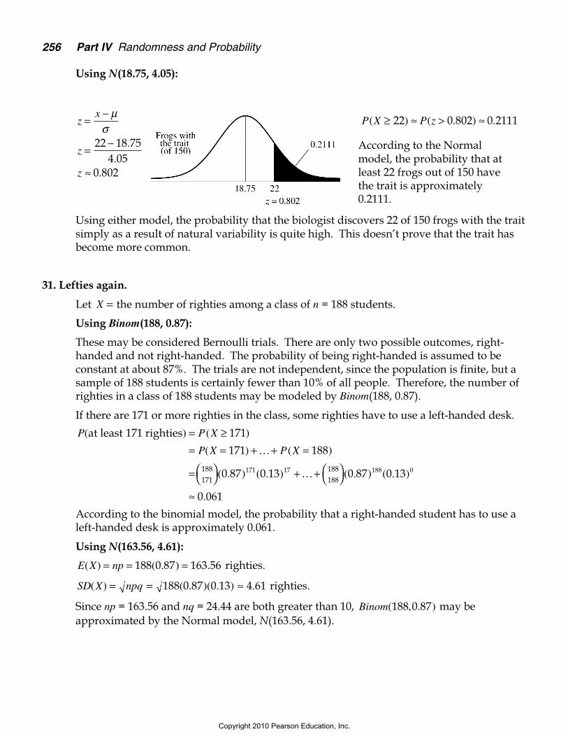
Using N(18.75, 4.05):
Using either model, the probability that the biologist discovers 22 of 150 frogs with the traitsimply as a result of natural variability is quite high. This doesn’t prove that the trait hasbecome more common.
31. Lefties again.
Let X = the number of righties among a class of n = 188 students.
Using Binom(188, 0.87):
These may be considered Bernoulli trials. There are only two possible outcomes, right-handed and not right-handed. The probability of being right-handed is assumed to beconstant at about 87%. The trials are not independent, since the population is finite, but asample of 188 students is certainly fewer than 10% of all people. Therefore, the number ofrighties in a class of 188 students may be modeled by Binom(188, 0.87).
If there are 171 or more righties in the class, some righties have to use a left-handed desk.
P P X
P X P X
( ( )
( ) ( )
( . ) ( . ) ( . ) ( . )
.
at least 171 righties ) = ≥= = + + =
=
+ +
≈
171
171 188
0 87 0 13 0 87 0 13
0 061
188171
188188
171 17 188 0
…
…
According to the binomial model, the probability that a right-handed student has to use aleft-handed desk is approximately 0.061.
Using N(163.56, 4.61):
E X np( ) ( . ) .= = =188 0 87 163 56 righties.
SD X npq( ) ( . )( . ) .= = ≈188 0 87 0 13 4 61 righties.
Since np = 163.56 and nq = 24.44 are both greater than 10, Binom( , . )188 0 87 may beapproximated by the Normal model, N(163.56, 4.61).
zx
z
z
=−
=−
≈
µσ
22 18 754 05
0 802
..
.
According to the Normalmodel, the probability that atleast 22 frogs out of 150 havethe trait is approximately0.2111.
P X P z( ) ( . ) .≥ ≈ > ≈22 0 802 0 2111
Copyright 2010 Pearson Education, Inc.
Chapter 17 Probability Models 257
32. No-shows.
Let X = the number of passengers that show up for the flight of n = 275 passengers.
Using Binom(275, 0.95):These may be considered Bernoulli trials. There are only two possible outcomes, showingup and not showing up. The airlines believe the probability of showing up is constant atabout 95%. The trials are not independent, since the population is finite, but a sample of275 passengers is certainly fewer than 10% of all passengers. Therefore, the number ofpassengers who show up for a flight of 275 may be modeled by Binom(275, 0.95).
If 266 or more passengers show up, someone has to get bumped off the flight.
P P X
P X P X
( ( )
( ) ( )
( . ) ( . ) ( . ) ( . )
.
at least 266 passengers ) = ≥= = + + =
=
+ +
≈
266
266 275
0 95 0 05 0 95 0 05
0 116
275266
275275
266 9 275 0
…
…
According to the binomial model, the probability someone on the flight must be bumped isapproximately 0.116.
Using N(261.25, 3.61):
E X np( ) ( . ) .= = =275 0 95 261 25 passengers.
SD X npq( ) ( . )( . ) .= = ≈275 0 95 0 05 3 61 passengers.
Since np = 261.25 and nq = 13.75 are both greater than 10, Binom( , . )275 0 95 may beapproximated by the Normal model, N(261.25, 3.61).
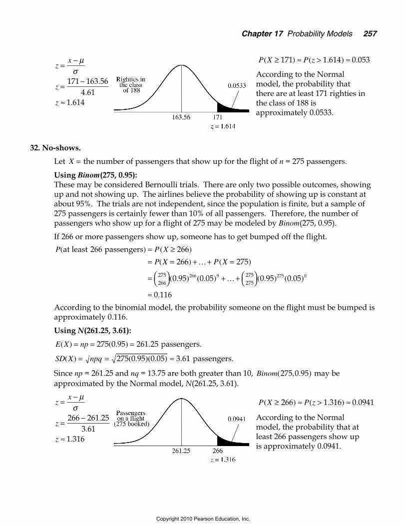
zx
z
z
=−
=−
≈
µσ
171 163 564 61
1 614
..
.
According to the Normalmodel, the probability thatthere are at least 171 righties inthe class of 188 isapproximately 0.0533.
P X P z( ) ( . ) .≥ ≈ > ≈171 1 614 0 053
zx
z
z
=−
=−
≈
µσ
266 261 253 61
1 316
..
.
According to the Normalmodel, the probability that atleast 266 passengers show upis approximately 0.0941.
P X P z( ) ( . ) .≥ ≈ > ≈266 1 316 0 0941
Copyright 2010 Pearson Education, Inc.
258 Part IV Randomness and Probability
33. Annoying phone calls.
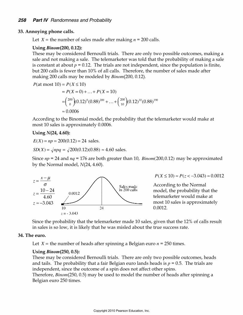
Let X = the number of sales made after making n = 200 calls.
Using Binom(200, 0.12):These may be considered Bernoulli trials. There are only two possible outcomes, making asale and not making a sale. The telemarketer was told that the probability of making a saleis constant at about p = 0.12. The trials are not independent, since the population is finite,but 200 calls is fewer than 10% of all calls. Therefore, the number of sales made aftermaking 200 calls may be modeled by Binom(200, 0.12).
P P X
P X P X
( ( )
( ) ( )
( . ) ( . ) ( . ) ( . )
.
at most 10 ) = ≤= = + + =
=
+ +
≈
100 10
0 12 0 88 0 12 0 88
0 0006
2000
20010
0 200 10 190
…
…
According to the Binomial model, the probability that the telemarketer would make atmost 10 sales is approximately 0.0006.
Using N(24, 4.60):
E X np( ) ( . )= = =200 0 12 24 sales.
SD X npq( ) ( . )( . ) .= = ≈200 0 12 0 88 4 60 sales.
Since np = 24 and nq = 176 are both greater than 10, Binom( , . )200 0 12 may be approximatedby the Normal model, N(24, 4.60).
Since the probability that the telemarketer made 10 sales, given that the 12% of calls resultin sales is so low, it is likely that he was misled about the true success rate.
34. The euro.
Let X = the number of heads after spinning a Belgian euro n = 250 times.
Using Binom(250, 0.5):These may be considered Bernoulli trials. There are only two possible outcomes, headsand tails. The probability that a fair Belgian euro lands heads is p = 0.5. The trials areindependent, since the outcome of a spin does not affect other spins.Therefore, Binom(250, 0.5) may be used to model the number of heads after spinning aBelgian euro 250 times.
zx
z
z
=−
=−
≈ −
µσ
10 244 603 043
..
According to the Normalmodel, the probability that thetelemarketer would make atmost 10 sales is approximately0.0012.
P X P z( ) ( . ) .≤ ≈ < − ≈10 3 043 0 0012
Copyright 2010 Pearson Education, Inc.
Chapter 17 Probability Models 259
P P X
P X P X
( ( )
( ) ( )
( . ) ( . ) ( . ) ( . )
.
at least 140 ) = ≥= = + + =
=
+ +
≈
140140 250
0 5 0 5 0 5 0 5
0 0332
250140
250250
140 110 250 0
…
…
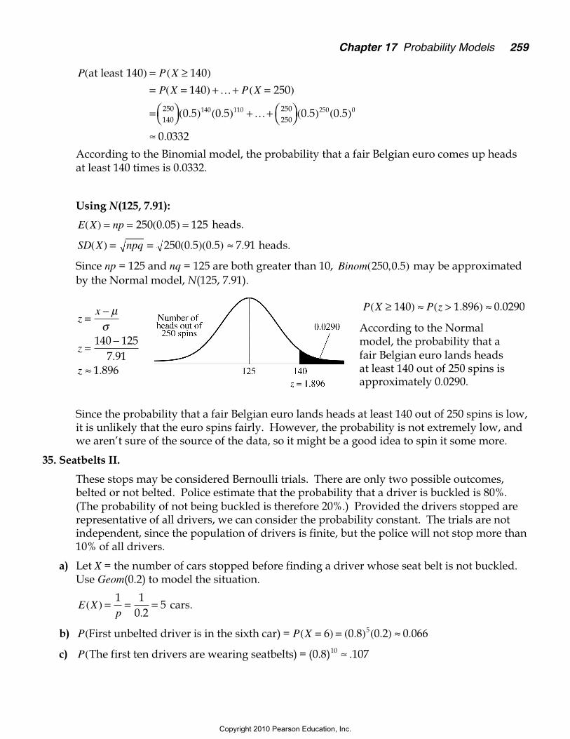
According to the Binomial model, the probability that a fair Belgian euro comes up headsat least 140 times is 0.0332.
Using N(125, 7.91):
E X np( ) ( . )= = =250 0 05 125 heads.
SD X npq( ) ( . )( . ) .= = ≈250 0 5 0 5 7 91 heads.
Since np = 125 and nq = 125 are both greater than 10, Binom( , . )250 0 5 may be approximatedby the Normal model, N(125, 7.91).
Since the probability that a fair Belgian euro lands heads at least 140 out of 250 spins is low,it is unlikely that the euro spins fairly. However, the probability is not extremely low, andwe aren’t sure of the source of the data, so it might be a good idea to spin it some more.
35. Seatbelts II.
These stops may be considered Bernoulli trials. There are only two possible outcomes,belted or not belted. Police estimate that the probability that a driver is buckled is 80%.(The probability of not being buckled is therefore 20%.) Provided the drivers stopped arerepresentative of all drivers, we can consider the probability constant. The trials are notindependent, since the population of drivers is finite, but the police will not stop more than10% of all drivers.
a) Let X = the number of cars stopped before finding a driver whose seat belt is not buckled.Use Geom(0.2) to model the situation.
E Xp
( ).
= = =1 1
0 25 cars.
b) P P X( ( ) ( . ) ( . ) .First unbelted driver is in the sixth car ) = = = ≈6 0 8 0 2 0 0665
c) P( .The first ten drivers are wearing seatbelts ) = (0.8)10 ≈ 107
zx
z
z
=−
=−
≈
µσ
140 1257 91
1 896.
.
According to the Normalmodel, the probability that afair Belgian euro lands headsat least 140 out of 250 spins isapproximately 0.0290.
P X P z( ) ( . ) .≥ ≈ > ≈140 1 896 0 0290
Copyright 2010 Pearson Education, Inc.
260 Part IV Randomness and Probability
d) Let Y = the number of drivers wearing their seatbelts in 30 cars. Use Binom(30, 0.8).
E Y np( ) ( . )= = =30 0 8 24 drivers.
SD Y npq( ) ( . )( . ) .= = ≈30 0 8 0 2 2 19 drivers.
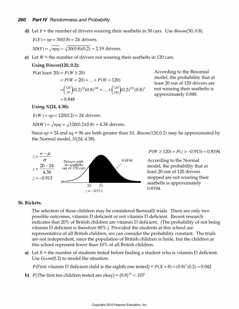
e) Let W = the number of drivers not wearing their seatbelts in 120 cars.
Using Binom(120, 0.2):
P P W
P W P W
( ( )
( ) ( )
( . ) ( . ) ( . ) ( . )
.
at least 20 ) = ≥= = + + =
=
+ +
≈
2020 120
0 2 0 8 0 2 0 8
0 848
12020
120120
20 100 120 0
…
…
Using N(24, 4.38):
E W np( ) ( . )= = =120 0 2 24 drivers.
SD W npq( ) ( . )( . ) .= = ≈120 0 2 0 8 4 38 drivers.
Since np = 24 and nq = 96 are both greater than 10, Binom( , . )120 0 2 may be approximated bythe Normal model, N(24, 4.38).
36. Rickets.
The selection of these children may be considered Bernoulli trials. There are only twopossible outcomes, vitamin D deficient or not vitamin D deficient. Recent researchindicates that 20% of British children are vitamin D deficient. (The probability of not beingvitamin D deficient is therefore 80%.) Provided the students at this school arerepresentative of all British children, we can consider the probability constant. The trialsare not independent, since the population of British children is finite, but the children atthis school represent fewer than 10% of all British children.
a) Let X = the number of students tested before finding a student who is vitamin D deficient.Use Geom(0.2) to model the situation.
P P X( ( ) ( . ) ( . ) .First vitamin D deficient child is the eighth one tested ) = = = ≈8 0 8 0 2 0 0427
b) P( .The first ten children tested are okay ) = (0.8)10 ≈ 107
According to the Binomialmodel, the probability that atleast 20 out of 120 drivers arenot wearing their seatbelts isapproximately 0.848.
zw
z
z
=−
=−
≈ −
µσ
20 244 380 913
..
According to the Normalmodel, the probability that atleast 20 out of 120 driversstopped are not wearing theirseatbelts is approximately0.8194.
P W P z( ) ( . ) .≥ ≈ > − ≈120 0 913 0 8194
Copyright 2010 Pearson Education, Inc.
Chapter 17 Probability Models 261
c) E Xp
( ).
= = =1 1
0 25 kids.
d) Let Y = the number of children who are vitamin D deficient out of 50 children.Use Binom(50, 0.2).
E Y np( ) ( . )= = =50 0 2 10 children. SD Y npq( ) ( . )( . ) .= = ≈50 0 2 0 8 2 83 children.
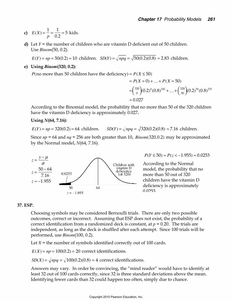
e) Using Binom(320, 0.2):
P P X
P X P X
( ( )
( ) ( )
( . ) ( . ) ( . ) ( . )
.
no more than 50 children have the deficiency ) = ≤= = + + =
=
+ +
≈
50
0 50
0 2 0 8 0 2 0 8
0 027
3200
32050
0 320 50 270
…
…
According to the Binomial model, the probability that no more than 50 of the 320 childrenhave the vitamin D deficiency is approximately 0.027.
Using N(64, 7.16):
E Y np( ) ( . )= = =320 0 2 64 children. SD Y npq( ) ( . )( . ) .= = ≈320 0 2 0 8 7 16 children.
Since np = 64 and nq = 256 are both greater than 10, Binom( , . )320 0 2 may be approximatedby the Normal model, N(64, 7.16).
37. ESP.
Choosing symbols may be considered Bernoulli trials. There are only two possibleoutcomes, correct or incorrect. Assuming that ESP does not exist, the probability of acorrect identification from a randomized deck is constant, at p = 0.20. The trials areindependent, as long as the deck is shuffled after each attempt. Since 100 trials will beperformed, use Binom(100, 0.2).
Let X = the number of symbols identified correctly out of 100 cards.
E X np( ) ( . )= = =100 0 2 20 correct identifications.
SD X npq( ) ( . )( . )= = =100 0 2 0 8 4 correct identifications.
Answers may vary. In order be convincing, the “mind reader” would have to identify atleast 32 out of 100 cards correctly, since 32 is three standard deviations above the mean.Identifying fewer cards than 32 could happen too often, simply due to chance.
zy
z
z
=−
=−
≈ −
µσ
50 647 161 955
..
According to the Normalmodel, the probability that nomore than 50 out of 320children have the vitamin Ddeficiency is approximately0.0253.
P Y P z( ) ( . ) .≤ ≈ < − ≈50 1 955 0 0253
Copyright 2010 Pearson Education, Inc.
262 Part IV Randomness and Probability
38. True-False.
Guessing at answers may be considered Bernoulli trials. There are only two possibleoutcomes, correct or incorrect. If the student was guessing, the probability of a correctresponse is constant, at p = 0.50. The trials are independent, since the answer to onequestion should not have any bearing on the answer to the next. Since 50 questions are onthe test use Binom(500, 0.5).
Let X = the number of questions answered correctly out of 50 questions.
E X np( ) ( . )= = =50 0 5 25 correct answers.
SD X npq( ) ( . )( . ) .= = ≈50 0 5 0 5 3 54 correct answers.
Answers may vary. In order be convincing, the student would have to answer at least 36out of 50 questions correctly, since 36 is approximately three standard deviations above themean. Answering fewer than 36 questions correctly could happen too often, simply due tochance.
39. Hot hand.
A streak like this is not unusual. The probability that he makes 4 in a row with a 55% freethrow percentage is ( . )( . )( . )( . ) .0 55 0 55 0 55 0 55 0 09≈ . We can expect this to happen nearly onein ten times for every set of 4 shots that he makes. One out of ten times is not that unusual.
40. New bow.
A streak like this is not unusual. The probability that she makes 6 consecutive bulls-eyeswith an 80% bulls-eye percentage is ( . )( . )( . )( . )( . )( . ) .0 8 0 8 0 8 0 8 0 8 0 8 0 26≈ . If she were to shootseveral flights of 6 arrows, she is expected to get 6 bulls-eyes about 26% of the time. Anevent that happens due to chance about one out of four times is not that unusual.
41. Hotter hand.
The shots may be considered Bernoulli trials. There are only two possible outcomes, makeor miss. The probability of success is constant at 55%, and the shots are independent of oneanother. Therefore, we can model this situation with Binom(32, 0.55).
Let X = the number of free throws made out of 40.
E X np( ) ( . )= = =40 0 55 22 free throws made.
SD X npq( ) ( . )( . ) .= = ≈40 0 55 0 45 3 15 free throws.
Answers may vary. The player’s performance seems to have increased. 32 made freethrows is ( ) / . .32 22 3 15 3 17− ≈ standard deviations above the mean, an extraordinary feat,unless his free throw percentage has increased. This does NOT mean that the sneakers areresponsible for the increase in free throw percentage. Some other variable may account forthe increase. The player would need to set up a controlled experiment in order todetermine what effect, if any, the sneakers had on his free throw percentage.
Copyright 2010 Pearson Education, Inc.
Chapter 17 Probability Models 263
42. New bow, again.
The shots may be considered Bernoulli trials. There are only two possible outcomes, hit ormiss the bulls-eye. The probability of success is constant at 80%, and the shots areindependent of one another. Therefore, we can model this situation with Binom(50, 0.8).
Let X = the number of bulls-eyes hit out of 50.
E X np( ) ( . )= = =50 0 8 40 bulls-eyes hit.
SD X npq( ) ( . )( . ) .= = ≈50 0 8 0 2 2 83 bulls-eyes.
Answers may vary. The archer’s performance doesn’t seem to have increased.45 bulls-eyes is ( ) / . .45 40 2 83 1 77− ≈ standard deviations above the mean. This isn’tunusual for an archer of her skill level.
Copyright 2010 Pearson Education, Inc.