Embed Size (px)
Citation preview
WinFrog User’s Guide – USBL Calibration 16-1
Chapter 16: USBL Calibration
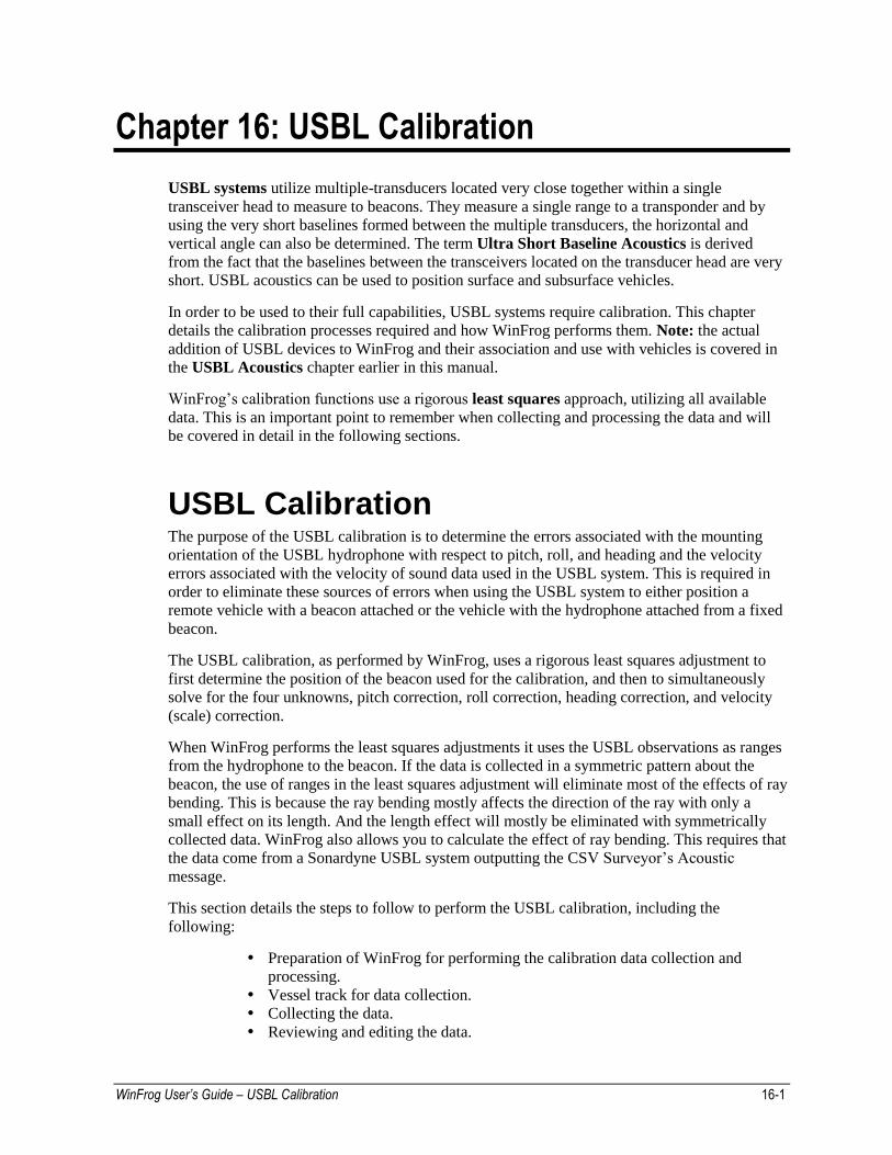
USBL systems utilize multiple-transducers located very close together within a single
transceiver head to measure to beacons. They measure a single range to a transponder and by
using the very short baselines formed between the multiple transducers, the horizontal and
vertical angle can also be determined. The term Ultra Short Baseline Acoustics is derived
from the fact that the baselines between the transceivers located on the transducer head are very
short. USBL acoustics can be used to position surface and subsurface vehicles.
In order to be used to their full capabilities, USBL systems require calibration. This chapter
details the calibration processes required and how WinFrog performs them. Note: the actual
addition of USBL devices to WinFrog and their association and use with vehicles is covered in
the USBL Acoustics chapter earlier in this manual.
WinFrog’s calibration functions use a rigorous least squares approach, utilizing all available
data. This is an important point to remember when collecting and processing the data and will
be covered in detail in the following sections.
USBL Calibration The purpose of the USBL calibration is to determine the errors associated with the mounting
orientation of the USBL hydrophone with respect to pitch, roll, and heading and the velocity
errors associated with the velocity of sound data used in the USBL system. This is required in
order to eliminate these sources of errors when using the USBL system to either position a
remote vehicle with a beacon attached or the vehicle with the hydrophone attached from a fixed
beacon.
The USBL calibration, as performed by WinFrog, uses a rigorous least squares adjustment to
first determine the position of the beacon used for the calibration, and then to simultaneously
solve for the four unknowns, pitch correction, roll correction, heading correction, and velocity
(scale) correction.
When WinFrog performs the least squares adjustments it uses the USBL observations as ranges
from the hydrophone to the beacon. If the data is collected in a symmetric pattern about the
beacon, the use of ranges in the least squares adjustment will eliminate most of the effects of ray
bending. This is because the ray bending mostly affects the direction of the ray with only a
small effect on its length. And the length effect will mostly be eliminated with symmetrically
collected data. WinFrog also allows you to calculate the effect of ray bending. This requires that
the data come from a Sonardyne USBL system outputting the CSV Surveyor’s Acoustic
message.
This section details the steps to follow to perform the USBL calibration, including the
following:
Preparation of WinFrog for performing the calibration data collection and
processing.
Vessel track for data collection.
Collecting the data.
Reviewing and editing the data.
16-2 WinFrog User’s Guide – USBL Calibration
Processing the calibration.
Application of the results.
Troubleshooting the process.
Reviewing and editing of the data and the processing is an iterative process.
Note: You can also use this technique to simply calculate the position of USBL
beacons. In this case, the differences between what is discussed in the remaining
part of this chapter and what would be required are the data collection pattern,
and the processing, which would stop once the beacon positions were
determined.
USBL Calibration Preparation In preparation for performing a USBL Calibration, WinFrog must be properly configured.
Although WinFrog provides recourse during processing to correct for omissions and errors in the
setup for the calibration, it is always better (and easier) to perform the setup correctly and
eliminate the need to use these features.
Key Points to Review Prior to USBL Calibration
1 It is important that the correct Working Transponder file is loaded and available prior to
the configuration for data collection. Check that there is a working file and it is the correct
one.
When performing the calibration and when operating the USBL for positioning (if fixed
beacons are being used), configure the Vehicle window to display the name of the Working
Transponder file.
2 The Transponder file must contain, at a minimum, the beacon that is to be used for the
calibration, the initial approximate position and depth for this beacon, and if the Sonardyne
CSV acoustic message is used then the beacon turn around time must be entered. The depth
is important because it is involved in the reduction of the observations to the map grid.
Depths for the beacon can be determined using depth interrogations, if it is equipped with a
depth sensor. Alternatively, the ship can pass directly over the deployment position while
ranging to the beacon and the shortest range can be used for the depth. Other options
include using a sounder or from a chart.
Note: A working velocity file is only required if the travel time from the USBL system is to
be used, such as the Sonardyne CSV acoustic message or Simrad $---SSB telegrams.
Otherwise, the velocity is entered into the USBL system itself.
3 Ensure that all positioning and related devices are correctly configured, including
operational settings and sensor offsets. These devices must be active and receiving data. If
new data are not present for any POSITION or USBL device that is attached to the
calibration vehicle, no calibration data will be collected. The USBL HYDROPHONE data
item must be attached to the vehicle being used for the calibration.
If an attitude sensor is present it must be injected directly into the USBL system. WinFrog
does not currently support application of attitude data to USBL data or sensor offsets. Note
that this is the only device for which this is true, all other devices and offsets support
application of attitude data.
WinFrog User’s Guide – USBL Calibration 16-3
There may be offsets entered into the USBL system; you must check to see if these are
present. If they are present they must be entered into the USBL HYDROPHONE data item
configuration dialog (>Configure Transducer 1>USBL System internal offsets). Note that
the signs must be correct. This is done so that the leaver arm from the USBL’s offset point
to the transceiver is corrected for attitude. i.e., WinFrog requires the beacon data relative to
the transceiver not an arbitrary point on the vessel.
NOTE: The USBL system must not be configured to operate in Fixed Beacon Depth or
Telemetered Beacon Depth mode, or similar. The Z component as determined from the
analysis of the return signal at the hydrophone head is critical for the USBL Corrections
Calibration process, in particular for the resolution for pitch and roll correction
determinations. The use of an operating mode that uses some other means of determining
the Z component will result in un-usable calibration data. It should be noted that once
observed and recorded, the data cannot be re-engineered to make it usable.
4 It is strongly recommended that the USBL HYDROPHONE data item always be configured
to Positioning - Secondary. While it can, in most cases, be configured to Positioning -
Primary without affecting the data collection and subsequent processing, there are
situations (discussed later) that require it be set to Secondary. Another consideration is that
when set to Positioning – Primary, WinFrog will use the USBL to compute the position of
the vessel. Since this determination will be based upon an estimated position for the fixed
beacon, and USBL is less accurate then the DGPS likely used, it will result in a jump in the
vehicle’s position. This situation may cause alarm among personnel, such as the helmsman,
who are using the WinFrog screens.
5 The computer directories should be setup such that the calibration data have a specific
location to which they are saved. The saving and archival process for the files should be
decided upon to ensure that the necessary steps are followed to ensure safe file saving and
archiving.
6 The USBL beacon used for the calibration should be deployed in an area that will permit
adequate maneuverability to perform the data collection pattern.
The Acoustic Calibration Dialog for Data Collection The Acoustic Calibration dialog, from which all data collection, saving, loading, editing,
processing, and reporting is performed, can be accessed in several ways.
To Access the Acoustic Calibration Dialog
1 Set the Vehicle Text window to display the information for the vehicle to which the USBL
Hydrophone is attached.
2 With the cursor in the Vehicle Text window, right-click to access the pop-up menu.
3 Select Acoustic Calibration.
Or
4 From the Main Menu, select Configure > Vehicles.
5 Highlight the vehicle to which the USBL Hydrophone is attached, and click the Acoustic
Calibration button.
16-4 WinFrog User’s Guide – USBL Calibration
Or
6 From the Acoustic Window, click on Configure > Select Vehicle for Calibration, then
click on the vehicle to which the USBL Hydrophone is attached.
7 Then click on Configure > Calibration.
Note: WinFrog is a multi-vehicle system. Ensure the vehicle that has the USBL
HYDROPHONE data item added to it is the one selected/displayed before clicking the Cal
button or using the right mouse button to access the pop-up menu. Normally this is not a
problem as the button is disabled or the menu item isn’t available, however, it may be enabled if
another acoustic data item is present, such as LBL HYDROPHONE. If the incorrect vehicle is
selected and the Calibration dialog is accessed, you will still be permitted to setup the
calibration data collection, but no data will be collected because no USBL data items are
associated with that vehicle. If it appears that no data are being collected, check for this
problem.
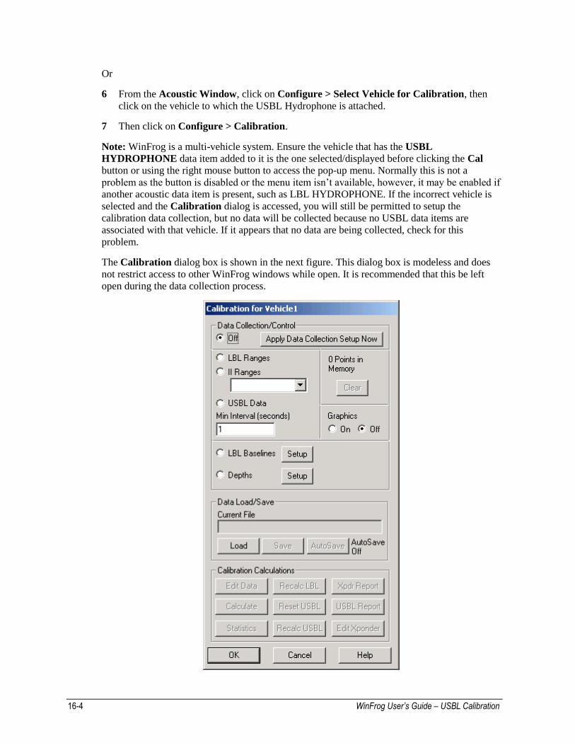
The Calibration dialog box is shown in the next figure. This dialog box is modeless and does
not restrict access to other WinFrog windows while open. It is recommended that this be left
open during the data collection process.
WinFrog User’s Guide – USBL Calibration 16-5
The following details those controls associated with the USBL Calibration data collection
process.
Note: The first time this dialog is opened for a vehicle, it creates a calibration data set
including a copy of the information from the working transponder file. Each subsequent time
the Calibration dialog is opened, WinFrog compares the current Working Transponder file
against the transponder station information contained in the Calibration data set and informs
you of differences between the Working Transponder file and the Calibration Transponder
station data (coordinate variations and discrepancies in stations). You can then decide
whether to overwrite the Calibration data set station information with that from the Working
Transponder file, or ignore the differences and keep the Calibration data set station
information untouched.
Data Collection Control
You control the type of data to collect with the controls in this section. Once selected, the
Apply… button will change to reflect the changes that will be applied if it is clicked.
Alternatively, selecting the data collection type and exiting the dialog with OK will also
apply the settings.
Off Stops data collection
LBL Ranges Not applicable to USBL.
II Ranges Not applicable to USBL.
USBL Data Turns on the collection of USBL data. This is
applicable for all USBL systems.
Min Interval This controls the minimum data collection
interval, in seconds, for the USBL data. During
data collection, WinFrog checks for the presence
of new data from the associated devices and then
checks to see if the minimum interval has been
reached or exceeded, and if so, logs the data. If
either of the preceding checks fails, no data are
logged.
LBL Baselines Not applicable to USBL.
Depths Not applicable to USBL.
Apply… button The text of this button displays the collection
setup that will be applied when clicked. Click this
button to cause the current Data Collection
setting(s) to be applied without having to close the
dialog.
Points In Memory The total number of points currently
loaded/present in WinFrog memory. It is very
important to note that when collecting
calibration data, WinFrog logs the data to
memory and not directly to disk. It is only
written to disk when specifically directed by the
operator.
Clear This will clear the current calibration data in
memory. Note: if these data have not been saved
to disk, they are not recoverable after this is
16-6 WinFrog User’s Guide – USBL Calibration
executed. A confirmation prompt appears when
the Clear button is clicked.
Graphics On/Off Controls the display of the data collection
positions in the Graphics and Bird’s Eye
windows. Thus, the Graphics display provides
both a means for monitoring the progress of the
data collection and clear illustration of the
geometry. After setting this option, the Apply…
button must be clicked or the dialog exited with
OK in order for the changes to take affect. You
may also have to refresh the graphics window by
resizing.
Data Load/Save
Current File This is a read only control giving the path and
name of the currently loaded calibration file or
the last one that had been in WinFrog memory.
Load Enables the browsing of available storage media
to select a calibration file (*.cal) and load it into
memory. Note: this action automatically clears
all calibration data currently in memory. You are
warned of this and are given the option to cancel
the action. You are also prompted as to whether
or not you wish to purge the current Calibration
data set transponder information. If there is a
difference between the station information of the
Calibration data being loaded and the current
Working Transponder file, you are informed of
this and given the option to overwrite the
Calibration data set station information from the
Working Transponder file or ignore the
difference.
Save This is only available if there are calibration data
in memory.
Enables browsing of available storage media to
select an existing file or enter a new file name to
save all the data currently in memory to disk.
Note: when data are saved to an existing file,
that file’s contents are replaced with the contents
of the memory. When this option is accessed and
USBL data is present, you are prompted for the
file format to use. The next figure shows the
available options.
WinFrog User’s Guide – USBL Calibration 16-7
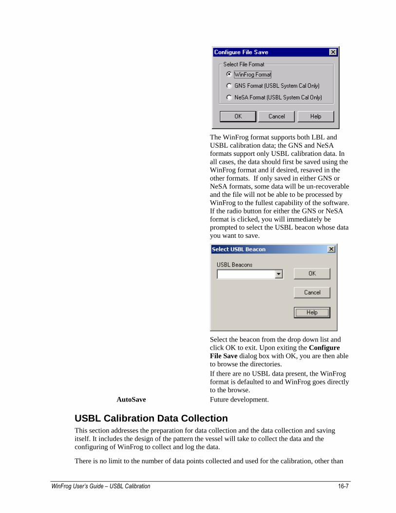
The WinFrog format supports both LBL and
USBL calibration data; the GNS and NeSA
formats support only USBL calibration data. In
all cases, the data should first be saved using the
WinFrog format and if desired, resaved in the
other formats. If only saved in either GNS or
NeSA formats, some data will be un-recoverable
and the file will not be able to be processed by
WinFrog to the fullest capability of the software.
If the radio button for either the GNS or NeSA
format is clicked, you will immediately be
prompted to select the USBL beacon whose data
you want to save.
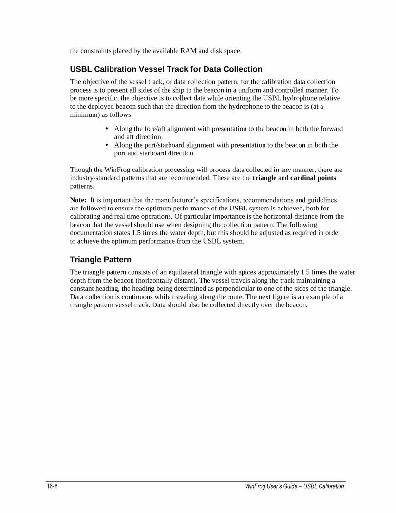
Select the beacon from the drop down list and
click OK to exit. Upon exiting the Configure
File Save dialog box with OK, you are then able
to browse the directories.
If there are no USBL data present, the WinFrog
format is defaulted to and WinFrog goes directly
to the browse.
AutoSave Future development.
USBL Calibration Data Collection This section addresses the preparation for data collection and the data collection and saving
itself. It includes the design of the pattern the vessel will take to collect the data and the
configuring of WinFrog to collect and log the data.
There is no limit to the number of data points collected and used for the calibration, other than
16-8 WinFrog User’s Guide – USBL Calibration
the constraints placed by the available RAM and disk space.
USBL Calibration Vessel Track for Data Collection
The objective of the vessel track, or data collection pattern, for the calibration data collection
process is to present all sides of the ship to the beacon in a uniform and controlled manner. To
be more specific, the objective is to collect data while orienting the USBL hydrophone relative
to the deployed beacon such that the direction from the hydrophone to the beacon is (at a
minimum) as follows:
Along the fore/aft alignment with presentation to the beacon in both the forward
and aft direction.
Along the port/starboard alignment with presentation to the beacon in both the
port and starboard direction.
Though the WinFrog calibration processing will process data collected in any manner, there are
industry-standard patterns that are recommended. These are the triangle and cardinal points
patterns.
Note: It is important that the manufacturer’s specifications, recommendations and guidelines
are followed to ensure the optimum performance of the USBL system is achieved, both for
calibrating and real time operations. Of particular importance is the horizontal distance from the
beacon that the vessel should use when designing the collection pattern. The following
documentation states 1.5 times the water depth, but this should be adjusted as required in order
to achieve the optimum performance from the USBL system.
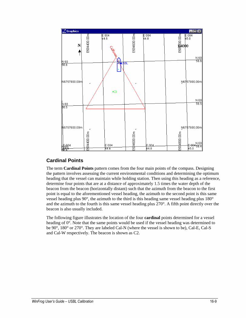
Triangle Pattern
The triangle pattern consists of an equilateral triangle with apices approximately 1.5 times the water
depth from the beacon (horizontally distant). The vessel travels along the track maintaining a
constant heading, the heading being determined as perpendicular to one of the sides of the triangle.
Data collection is continuous while traveling along the route. The next figure is an example of a
triangle pattern vessel track. Data should also be collected directly over the beacon.
WinFrog User’s Guide – USBL Calibration 16-9
Cardinal Points
The term Cardinal Points pattern comes from the four main points of the compass. Designing
the pattern involves assessing the current environmental conditions and determining the optimum
heading that the vessel can maintain while holding station. Then using this heading as a reference,
determine four points that are at a distance of approximately 1.5 times the water depth of the
beacon from the beacon (horizontally distant) such that the azimuth from the beacon to the first
point is equal to the aforementioned vessel heading, the azimuth to the second point is this same
vessel heading plus 90°, the azimuth to the third is this heading same vessel heading plus 180°
and the azimuth to the fourth is this same vessel heading plus 270°. A fifth point directly over the
beacon is also usually included.
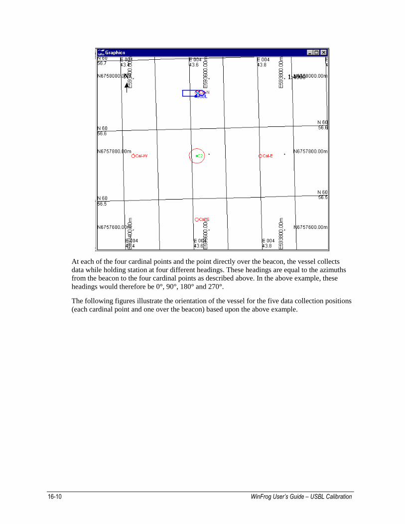
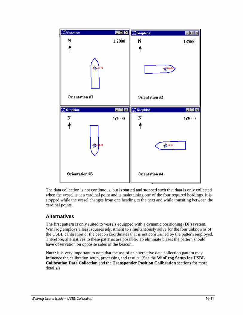
The following figure illustrates the location of the four cardinal points determined for a vessel
heading of 0°. Note that the same points would be used if the vessel heading was determined to
be 90°, 180° or 270°. They are labeled Cal-N (where the vessel is shown to be), Cal-E, Cal-S
and Cal-W respectively. The beacon is shown as C2.
16-10 WinFrog User’s Guide – USBL Calibration
At each of the four cardinal points and the point directly over the beacon, the vessel collects
data while holding station at four different headings. These headings are equal to the azimuths
from the beacon to the four cardinal points as described above. In the above example, these
headings would therefore be 0°, 90°, 180° and 270°.
The following figures illustrate the orientation of the vessel for the five data collection positions
(each cardinal point and one over the beacon) based upon the above example.
WinFrog User’s Guide – USBL Calibration 16-11
The data collection is not continuous, but is started and stopped such that data is only collected
when the vessel is at a cardinal point and is maintaining one of the four required headings. It is
stopped while the vessel changes from one heading to the next and while transiting between the
cardinal points.
Alternatives
The first pattern is only suited to vessels equipped with a dynamic positioning (DP) system.
WinFrog employs a least squares adjustment to simultaneously solve for the four unknowns of
the USBL calibration or the beacon coordinates that is not constrained by the pattern employed.
Therefore, alternatives to these patterns are possible. To eliminate biases the pattern should
have observation on opposite sides of the beacon.
Note: it is very important to note that the use of an alternative data collection pattern may
influence the calibration setup, processing and results. (See the WinFrog Setup for USBL
Calibration Data Collection and the Transponder Position Calibration sections for more
details.)
16-12 WinFrog User’s Guide – USBL Calibration
General
It should be noted that in the case of the triangle and cardinal points patterns, it is the relative
relationship and orientation between the vessel and the beacon that is important, not the absolute.
Thus, in the case of the triangle pattern, the triangle can be rotated to any orientation as long as
the vessel maintains the same heading (perpendicular to one leg of the triangle). Similarly, in the
case of the cardinal points pattern, the actual pattern could be rotated to any orientation as long as
the vessel’s headings at each collection point matched the azimuths from the beacon to each of
the points. This would hold true for an alternative pattern too.
WinFrog Setup for USBL Calibration Data Collection
This section explains the setup of WinFrog for the purpose of collecting data for a USBL
calibration. The assumption is made that the USBL device and other required devices have been
added to WinFrog and that the associated data items (USBL HYDROPHONE, POSITION,
HEADING, etc.) have been attached to the calibration vehicle.
USBL Hardware
The setup of the USBL system is important in order to obtain optimum results from the
calibration. The following steps must be followed.
1 If an attitude sensor is present, it must be injected directly into the USBL system. WinFrog
does not currently support application of attitude data to USBL data or USBL sensor
offsets. Note: this is the only device for which this is true, all other devices and offsets
support application of attitude data.
2 Offsets from the USBL system’s hydrophone to a reference point on the vessel must be
entered into the USBL system. In most cases, these are already present because they are
required to reference the data to the Center of Gravity (COG) of the vessel for output to a
Dynamic Positioning (DP) system. If this is not the case, offsets to the same Common
Reference Point (CRP) that will be used by WinFrog are to be entered, making sure that
the vertical reference is the waterline. This is done so that the leaver arm to the transceiver
is corrected for attitude, as well as the observations from the transceiver to the beacon.
3 The USBL system must not be configured to operate in Fixed Beacon Depth or
Telemetered Beacon Depth mode, or similar. The Z component as determined from the
analysis of the return signal at the hydrophone head is critical for the USBL Corrections
Calibration process, in particular for the resolution for pitch and roll correction
determinations. The use of an operating mode that uses some other means of determining
the Z component will result in un-usable calibration data. It should be noted that the data
cannot be re-engineered to make it usable.
4 The USBL systems may support the direct entry of USBL corrections. Since these are used
to correct the data prior to output to peripheral hardware, they can be left in the system and
the WinFrog calibration is then used to refine the corrections. This is particularly true for
corrections entered to correct for gross USBL installation errors, such as the mis-alignment
of the transducer head by 180°. WinFrog applies a rigorous least squares adjustment and
makes no assumptions that the corrections are small angles. However, it is unable to resolve
a heading error of 180°.
Note: due to the possibility of confusing sign conventions, it is recommended that the
results of the WinFrog USBL Calibration not be entered directly into a USBL system.
WinFrog User’s Guide – USBL Calibration 16-13
Rather, they should be entered and applied within WinFrog. The sign conventions used by
WinFrog and presented to you are provided in such a manner that the sign conventions are
easily followed. The WinFrog results of the calibration are entered into the WinFrog USBL
hydrophone configuration exactly as shown and printed.
Vehicle Configuration
The vehicle configuration consists of editing the data item’s associated with the calibration
vehicle. This is accomplished using that vehicle’s Configure Vehicle-Devices dialog.
It is recommended that the Kalman Filter be turned on and Dead Reckoning enabled for the
USBL Hydrophone vehicle.
Note: all POSITION and USBL HYDROPHONE data associated with the calibration vehicle
will be logged to the calibration file, along with general vehicle data. In addition, a standard
deviation is logged for each data item. This is used to determine the initial weighting for that
data item in the calibration processing (inverse of the standard deviation squared).
If a POSITION data item is configured as Primary its standard deviation is logged in the
calibration file. If a POSITION data item is configured as Secondary, the standard deviation
logged for that data item is 0 or Off. The standard deviation logged for the USBL
HYDROPHONE is the accuracy entered for this data item.
Note: it is recommended that the accuracy settings be “pessimistic” and relative with respect to
the different systems involved. Reasonable settings for a DGPS are 3 to 5 meters and 7 to 10
meters for a USBL system (HYDROPHONE and BEACON). The same relative relationship
should be maintained in real-time and calibration processing.
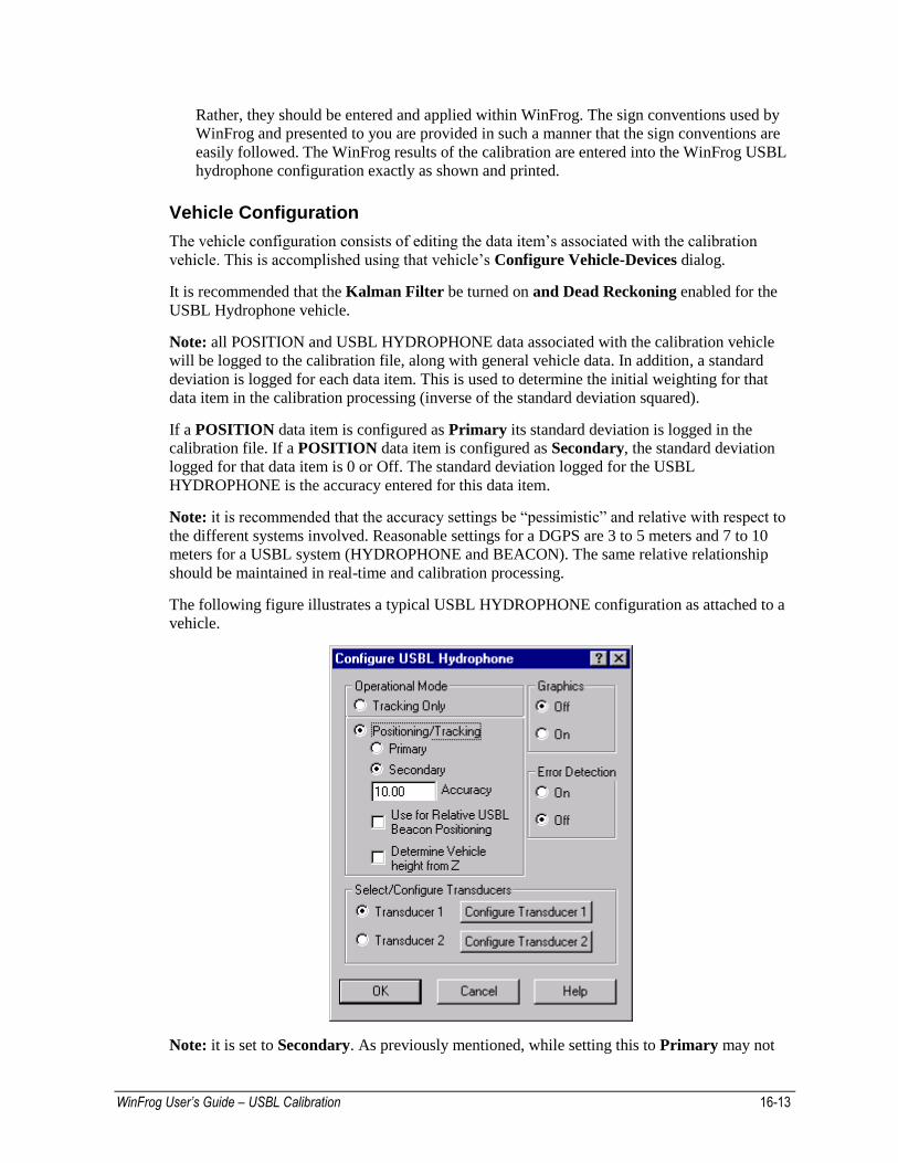
The following figure illustrates a typical USBL HYDROPHONE configuration as attached to a
vehicle.
Note: it is set to Secondary. As previously mentioned, while setting this to Primary may not
16-14 WinFrog User’s Guide – USBL Calibration
affect the calibration processing (see note below), it will affect the real-time positioning. If set
to Primary WinFrog will use the fixed beacon and USBL data to position the vessel. This will
likely produce inaccurate positioning with respect to DGPS and thus position jumps that may
result.
Note: a general procedural recommendation is that the USBL HYDROPHONE data item
always be set to Positioning - Secondary. If an alternative data collection pattern is used, it is
critical that the USBL HYDROPHONE data item be set to Secondary. If set to Secondary, you
are not constrained during the processing by an incorrect decision made at the data collection.
Though it will not affect the data collection, it is recommended that the Use for Relative USBL
Beacon Positioning and Determine Vehicle height from Z check boxes be unchecked.
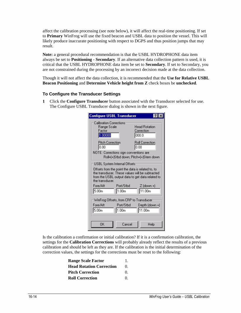
To Configure the Transducer Settings
1 Click the Configure Transducer button associated with the Transducer selected for use.
The Configure USBL Transducer dialog is shown in the next figure.
Is the calibration a confirmation or initial calibration? If it is a confirmation calibration, the
settings for the Calibration Corrections will probably already reflect the results of a previous
calibration and should be left as they are. If the calibration is the initial determination of the
correction values, the settings for the corrections must be reset to the following:
Range Scale Factor 1.
Head Rotation Correction 0.
Pitch Correction 0.
Roll Correction 0.
WinFrog User’s Guide – USBL Calibration 16-15
Note: during the calibration process you have recourse to reset the process, i.e., to revert to the
original raw data unaffected by any calibration corrections applied either at the time of data
collection or during the processing to that point. Therefore, an incorrect decision at this point is
not irreversible.
The offsets must also be confirmed to be correct. There are two sets of offsets to enter for a
USBL system. The first are the offsets currently entered into the USBL system itself to
reference the data to a specified vessel reference point (i.e. COG). Note the sign convention of
these offsets; the values are entered as measured from the said reference point to the transducer.
A vertical offset is positive if the transducer is below the reference point.
The second set of offsets are the standard WinFrog sensor offsets with the respective sign
convention, i.e. values are as measured from the CRP to the sensor and a vertical offset is
positive if the sensor is below the CRP. Remember, the WinFrog CRP must be at water level
and thus, the vertical offset is actually the draft of the transducer.
Note: there is no recourse to the entry of incorrect USBL system offsets within WinFrog once
the data is logged, i.e. if the offsets from the USBL reference point back to the transducer (as
entered directly into the USBL system) are incorrectly entered into WinFrog, the data can not be
used for the calibration. If this happens, the calibration data file can only be recovered through
manipulation using a spreadsheet program. There is however, recourse for the incorrect entry of
the WinFrog sensor offsets.
The previous figure is an example of the WinFrog CRP and the USBL system’s reference point
being, in fact, the same point.
To Collect USBL Calibration Data
The collection of the calibration data is controlled directly from the Acoustic Calibration
dialog.
1 Set the minimum data logging interval.
Since the only limit on the amount of data logged is the available computer memory and
available storage media space, it is better to set this interval fairly small. If too long, any
problems (i.e. acoustic noise) during the data collection may result in unacceptable gaps in the
designed collection track. It is easier to edit out data than wish there was more data present.
2 Toggle the USBL Data radio button.
3 Click the Apply button.
As points are collected, the Points in Memory text will update and, if the Graphics On is
selected, the data collection points will be displayed in the Graphics windows.
New data will not be collected until the minimum time has elapsed and then only when the
next new data are received for all USBL HYDROPHONE and POSITION devices attached
to the vehicle.
When the data collection is complete, or at any time the collection is to be suspended,
toggle the Off radio button and click the Apply button. It is important to note that the data
collection can be suspended and resumed at any time. This is particularly relevant when
using the cardinal points pattern.
16-16 WinFrog User’s Guide – USBL Calibration
WinFrog does not support the writing of the calibration data directly to disk as it is collected.
The saving of the calibration data to file is an operator-initiated action.
To Save Calibration Data to File
1 From the Acoustic Calibration dialog, click the Save button.
This can be performed at any time there are data present in memory. It is very strongly
recommended that the data be saved regularly to a file during the collection process.
Remember, as mentioned previously, when data are saved to an existing file, the contents of
that file are replaced with the complete data currently in memory. Thus, though this
provides an easy technique for repeatedly saving the data to the same file during the data
collection process, care must be exercised to ensure that the correct file is selected.
In addition, an existing data file can be loaded and data collection turned on to add more
calibration data.
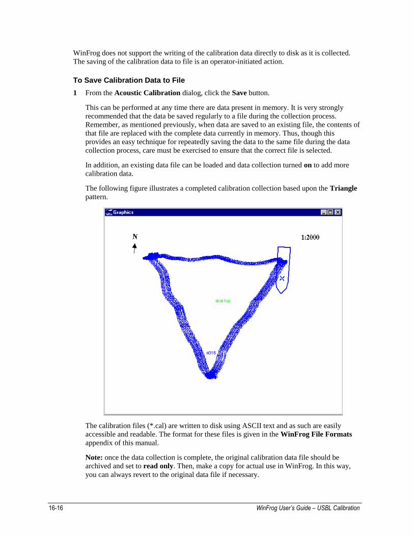
The following figure illustrates a completed calibration collection based upon the Triangle
pattern.
The calibration files (*.cal) are written to disk using ASCII text and as such are easily
accessible and readable. The format for these files is given in the WinFrog File Formats
appendix of this manual.
Note: once the data collection is complete, the original calibration data file should be
archived and set to read only. Then, make a copy for actual use in WinFrog. In this way,
you can always revert to the original data file if necessary.
WinFrog User’s Guide – USBL Calibration 16-17
USBL Data Collection - Monitoring
The number of points collected are displayed in the Calibration configuration dialog box.
However, the data collection process is best monitored with the Calibration Status window in
the Acoustic Window (see the Operator Display Windows chapter).
USBL Calibration Data Editing The data editing can be performed any time there are data available in WinFrog memory,
though it is generally done once the data collection process is complete.
The purpose of viewing and editing the data is to locate and remove those data that are
considered to be invalid. WinFrog provides you with graphical editors that enable easy
inspection of the data, detection of any trends, and direct editing capabilities. The graphical
editors allow you to view the LOP data directly and the LOP residuals. The former is best used
for investigating trends and visually detecting outliers, usually visible due to the associated
break in a trend, and thus, is a very important pre-processing tool. The latter is valuable for
refining the editing in subsequent iterations.
Note: the term editing the data consists of setting the weighting value for any given LOP and
changing data item offsets. You do not have access to the actual data for the purpose of altering
values.
An initial review of the data should be made prior to any calibration calculations. The purpose
of this review is to find obvious flyers and bad data and remove them from the solution
immediately. Then, after each calibration solution, the data should be viewed again for analysis
and any further required editing.
To View USBL Calibration Data for Editing
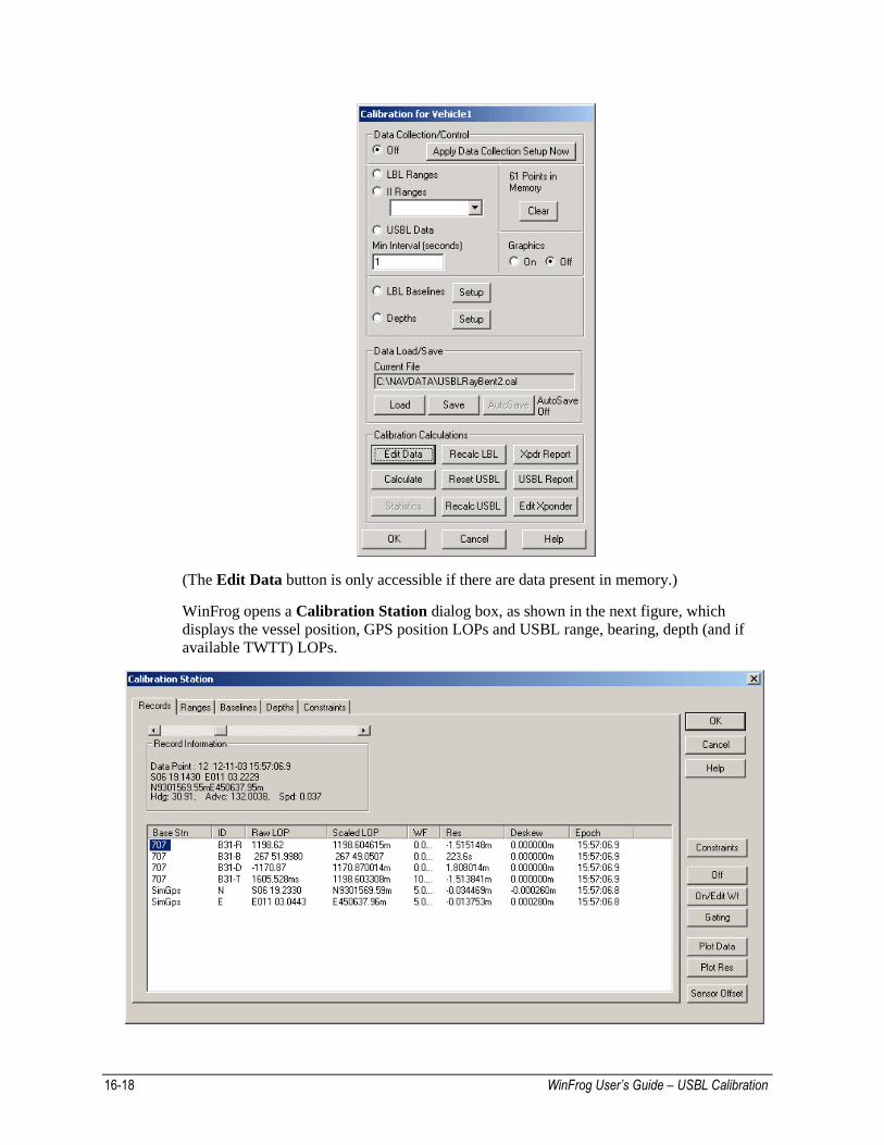
1 From the Calibration dialog box, click the Edit Data button.
16-18 WinFrog User’s Guide – USBL Calibration
(The Edit Data button is only accessible if there are data present in memory.)
WinFrog opens a Calibration Station dialog box, as shown in the next figure, which
displays the vessel position, GPS position LOPs and USBL range, bearing, depth (and if
available TWTT) LOPs.
WinFrog User’s Guide – USBL Calibration 16-19
Note: the example shown above includes four USBL based LOPs, R, B, D and T. The T
LOP is two-way-travel-time and is not available for all USBL devices. If it is not supported
by the respective USBL driver in WinFrog, this LOP is not displayed.
The Calibration Station dialog box presents you with several options for viewing the calibration
data. For a USBL Corrections calibration, generally only the Records and Ranges tab are
relevant. The available editing options accessed via the buttons located on the right side of the
dialog depend on the tab selected, and in the case of the Records tab, the type of LOP selected.
To edit an LOP, simply select it and click the appropriate button on the right. Make the editing
changes as required and exit the editing dialog with OK to save the editing changes or Cancel
to discard any changes made.
The following details the options available and the associated dialog boxes.
Off This simply sets the weighting factor for the
selected LOP to 0, which de-weights it from the
solution. This option is only available with the
Records and Constraints tabs. When associated
with a constraint, this toggles it between applied
and not applied.
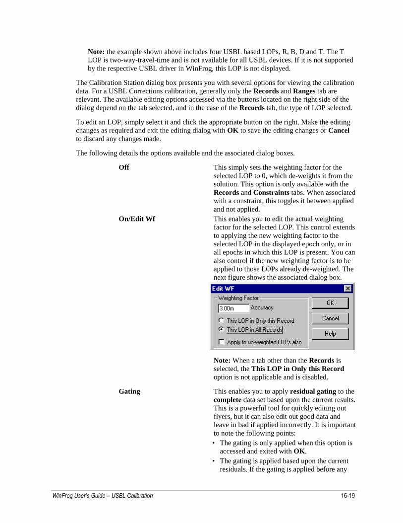
On/Edit Wf This enables you to edit the actual weighting
factor for the selected LOP. This control extends
to applying the new weighting factor to the
selected LOP in the displayed epoch only, or in
all epochs in which this LOP is present. You can
also control if the new weighting factor is to be
applied to those LOPs already de-weighted. The
next figure shows the associated dialog box.
Note: When a tab other than the Records is
selected, the This LOP in Only this Record
option is not applicable and is disabled.
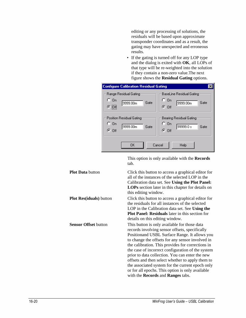
Gating This enables you to apply residual gating to the
complete data set based upon the current results.
This is a powerful tool for quickly editing out
flyers, but it can also edit out good data and
leave in bad if applied incorrectly. It is important
to note the following points:
• The gating is only applied when this option is
accessed and exited with OK.
• The gating is applied based upon the current
residuals. If the gating is applied before any
16-20 WinFrog User’s Guide – USBL Calibration
editing or any processing of solutions, the
residuals will be based upon approximate
transponder coordinates and as a result, the
gating may have unexpected and erroneous
results.
• If the gating is turned off for any LOP type
and the dialog is exited with OK, all LOPs of
that type will be re-weighted into the solution
if they contain a non-zero value.The next
figure shows the Residual Gating options.
This option is only available with the Records
tab.
Plot Data button Click this button to access a graphical editor for
all of the instances of the selected LOP in the
Calibration data set. See Using the Plot Panel:
LOPs section later in this chapter for details on
this editing window.
Plot Res(iduals) button Click this button to access a graphical editor for
the residuals for all instances of the selected
LOP in the Calibration data set. See Using the
Plot Panel: Residuals later in this section for
details on this editing window.
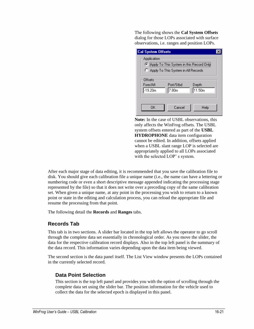
Sensor Offset button This button is only available for those data
records involving sensor offsets, specifically
Positionand USBL Surface Range. It allows you
to change the offsets for any sensor involved in
the calibration. This provides for corrections in
the case of incorrect configuration of the system
prior to data collection. You can enter the new
offsets and then select whether to apply them to
the associated system for the current epoch only
or for all epochs. This option is only available
with the Records and Ranges tabs.
WinFrog User’s Guide – USBL Calibration 16-21
The following shows the Cal System Offsets
dialog for those LOPs associated with surface
observations, i.e. ranges and position LOPs.
Note: In the case of USBL observations, this
only affects the WinFrog offsets. The USBL
system offsets entered as part of the USBL
HYDROPHONE data item configuration
cannot be edited. In addition, offsets applied
when a USBL slant range LOP is selected are
appropriately applied to all LOPs associated
with the selected LOP’ s system.
After each major stage of data editing, it is recommended that you save the calibration file to
disk. You should give each calibration file a unique name (i.e., the name can have a lettering or
numbering code or even a short descriptive message appended indicating the processing stage
represented by the file) so that it does not write over a preceding copy of the same calibration
set. When given a unique name, at any point in the processing you wish to return to a known
point or state in the editing and calculation process, you can reload the appropriate file and
resume the processing from that point.
The following detail the Records and Ranges tabs.
Records Tab
This tab is in two sections. A slider bar located in the top left allows the operator to go scroll
through the complete data set essentially in chronological order. As you move the slider, the
data for the respective calibration record displays. Also in the top left panel is the summary of
the data record. This information varies depending upon the data item being viewed.
The second section is the data panel itself. The List View window presents the LOPs contained
in the currently selected record.
Data Point Selection
This section is the top left panel and provides you with the option of scrolling through the
complete data set using the slider bar. The position information for the vehicle used to
collect the data for the selected epoch is displayed in this panel.
16-22 WinFrog User’s Guide – USBL Calibration
Line 1 The calibration point number and the date and
time for the selected point.
Line 2 The geographic coordinate for vehicle’s CRP on
the working ellipsoid.
Line 3 The map grid coordinate for the vehicle’s CRP.
Line 4 The vehicle’s heading, CMG, and speed in
knots.
Data Point Summary
This section is the lower, larger panel and presents the data (LOPs) collected at the selected
epoch in a list window. Note: there are no sort capabilities available, the data are displayed
in the order that the data items are added to the associated vehicle. It is also important to
note that the selection of an LOP is only possible from the first column. The order does not
affect the calibration processing. A single position data item provides two LOPs: a latitude
and a longitude. A USBL data item provides three LOPs: slope range, bearing, and depth.
Base Stn This lists the LOP’s name. In the case of a
position LOP, the name of the associated device
is shown, in the case of the USBL LOPs, the
name of the station is given.
ID This lists the associated ID of the LOP. In the
case of a position LOP, it is the denotation of
either N(orthing) or E(asting). In the case of a
USBL range LOP, it is the beacon ID with a
code identifying the LOP type:
R = Range, B = Bearing, D = Depth and T =
TWTT.
Raw LOP This is the raw LOP, or actual data, logged for
the LOP. For a position LOP it is the WGS 84
latitude and/or longitude. For USBL LOPs, they
are the raw slope range, bearing, depth and
TWTT as obtained from the USBL system
(corrected for the USBL system offsets).
Scaled LOP This is the scaled LOP, or data reduced to the
map projection. In the case of a position data
item, the WGS 84 position is transformed to the
working ellipsoid and then projected onto the
working map projection. For the USBL LOPs,
the data are projected onto the map grid and
corrected with the current USBL calibration
corrections, either as they were applied in real-
time (during data collection) or determined and
applied as part of the current calibration
processing.
WF This is the weighting factor used for the LOP in
the solution. Note: the lower the value, the
greater affect the LOP will have on the solution.
Res This is the residual for the LOP for the selected
epoch.
WinFrog User’s Guide – USBL Calibration 16-23
Deskew The individual LOPs collected for a given
calibration epoch are actually valid for different
times. The calibration point epoch is defined by
the vessel position epoch. Position LOPs are
deskewed to the vessel epoch using velocity
vectors generated as part of the standard real-
time positioning and processing and logged with
the calibration data. In the case of USBL LOPs,
the vessel position is dekewed to the USBL
epoch and as a result the deskew value for
USBL data is shown as 0 in this window. In fact,
the data capture and logging is driven by the
reception of the USBL data and as a result, if the
vehicle positioning is set to use Kalman Filter
and Dead Reckoning (recommended settings)
the vessel epoch and USBL data epoch will be
virtually the same.
Epoch This is the time stamp for the LOP data.
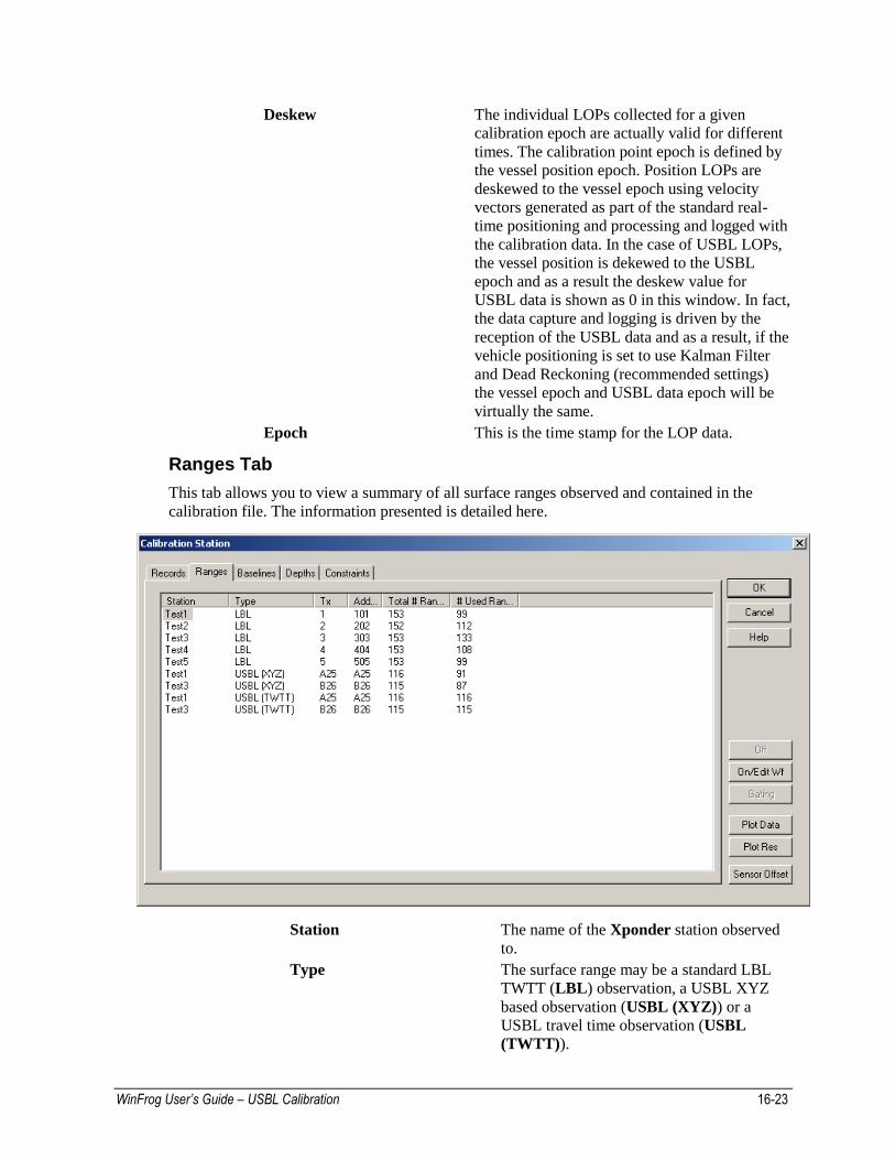
Ranges Tab
This tab allows you to view a summary of all surface ranges observed and contained in the
calibration file. The information presented is detailed here.
Station The name of the Xponder station observed
to.
Type The surface range may be a standard LBL
TWTT (LBL) observation, a USBL XYZ
based observation (USBL (XYZ)) or a
USBL travel time observation (USBL
(TWTT)).
16-24 WinFrog User’s Guide – USBL Calibration
Tx The transmit channel (or frequency) or
beacon ID of the Xponder station observed
to.
Address The address of the Xponder station
observed to, which in the case of a USBL
beacon duplicates the ID.
Total # Ranges The total number of observations made to
the Xponder station.
# Used Ranges The total number of observations made to
the Xponder station that are weighted into
the solution.
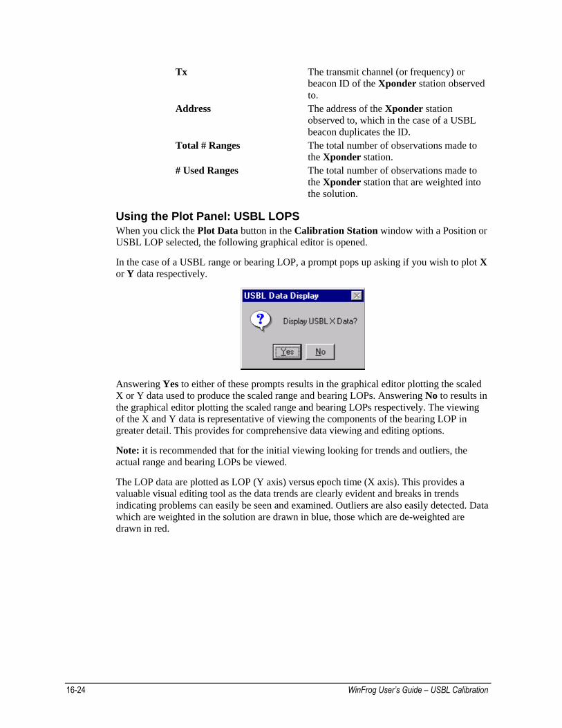
Using the Plot Panel: USBL LOPS
When you click the Plot Data button in the Calibration Station window with a Position or
USBL LOP selected, the following graphical editor is opened.
In the case of a USBL range or bearing LOP, a prompt pops up asking if you wish to plot X
or Y data respectively.
Answering Yes to either of these prompts results in the graphical editor plotting the scaled
X or Y data used to produce the scaled range and bearing LOPs. Answering No to results in
the graphical editor plotting the scaled range and bearing LOPs respectively. The viewing
of the X and Y data is representative of viewing the components of the bearing LOP in
greater detail. This provides for comprehensive data viewing and editing options.
Note: it is recommended that for the initial viewing looking for trends and outliers, the
actual range and bearing LOPs be viewed.
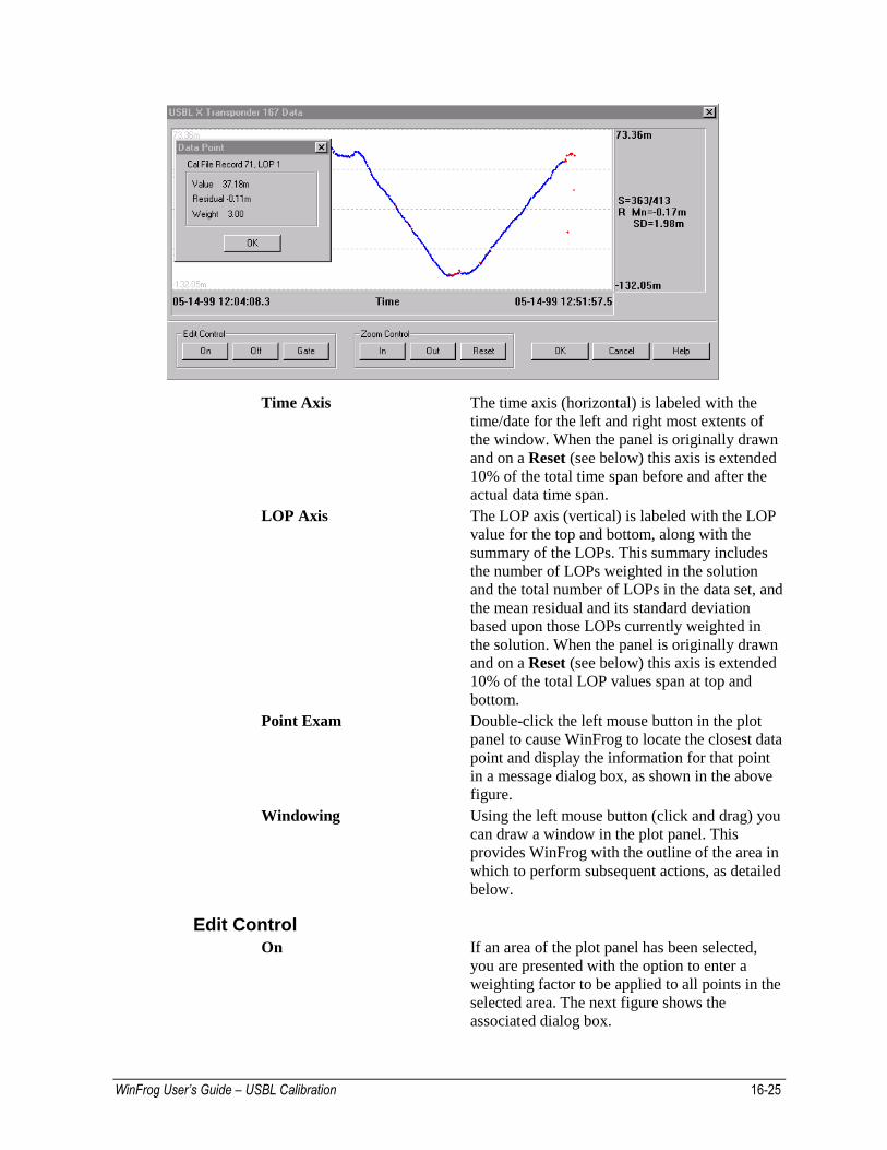
The LOP data are plotted as LOP (Y axis) versus epoch time (X axis). This provides a
valuable visual editing tool as the data trends are clearly evident and breaks in trends
indicating problems can easily be seen and examined. Outliers are also easily detected. Data
which are weighted in the solution are drawn in blue, those which are de-weighted are
drawn in red.
WinFrog User’s Guide – USBL Calibration 16-25
Time Axis The time axis (horizontal) is labeled with the
time/date for the left and right most extents of
the window. When the panel is originally drawn
and on a Reset (see below) this axis is extended
10% of the total time span before and after the
actual data time span.
LOP Axis The LOP axis (vertical) is labeled with the LOP
value for the top and bottom, along with the
summary of the LOPs. This summary includes
the number of LOPs weighted in the solution
and the total number of LOPs in the data set, and
the mean residual and its standard deviation
based upon those LOPs currently weighted in
the solution. When the panel is originally drawn
and on a Reset (see below) this axis is extended
10% of the total LOP values span at top and
bottom.
Point Exam Double-click the left mouse button in the plot
panel to cause WinFrog to locate the closest data
point and display the information for that point
in a message dialog box, as shown in the above
figure.
Windowing Using the left mouse button (click and drag) you
can draw a window in the plot panel. This
provides WinFrog with the outline of the area in
which to perform subsequent actions, as detailed
below.
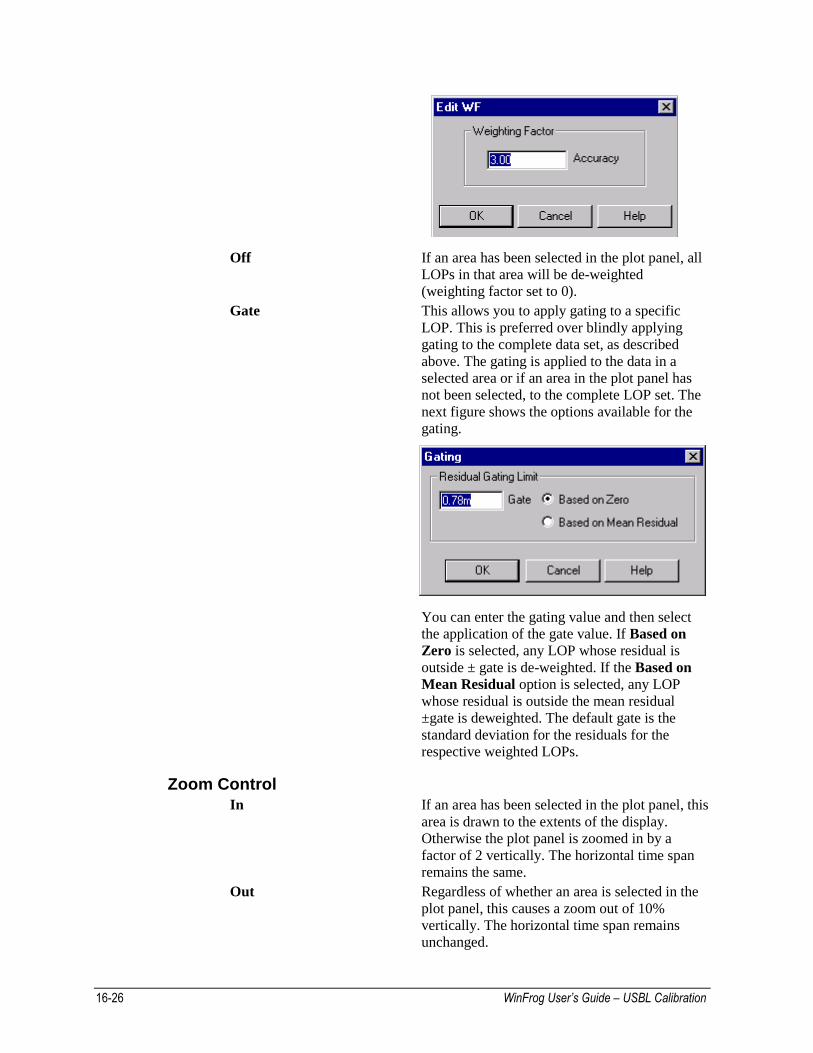
Edit Control
On If an area of the plot panel has been selected,
you are presented with the option to enter a
weighting factor to be applied to all points in the
selected area. The next figure shows the
associated dialog box.
16-26 WinFrog User’s Guide – USBL Calibration
Off If an area has been selected in the plot panel, all
LOPs in that area will be de-weighted
(weighting factor set to 0).
Gate This allows you to apply gating to a specific
LOP. This is preferred over blindly applying
gating to the complete data set, as described
above. The gating is applied to the data in a
selected area or if an area in the plot panel has
not been selected, to the complete LOP set. The
next figure shows the options available for the
gating.
You can enter the gating value and then select
the application of the gate value. If Based on
Zero is selected, any LOP whose residual is
outside ± gate is de-weighted. If the Based on
Mean Residual option is selected, any LOP
whose residual is outside the mean residual
±gate is deweighted. The default gate is the
standard deviation for the residuals for the
respective weighted LOPs.
Zoom Control
In If an area has been selected in the plot panel, this
area is drawn to the extents of the display.
Otherwise the plot panel is zoomed in by a
factor of 2 vertically. The horizontal time span
remains the same.
Out Regardless of whether an area is selected in the
plot panel, this causes a zoom out of 10%
vertically. The horizontal time span remains
unchanged.
WinFrog User’s Guide – USBL Calibration 16-27
Reset Re-draws the plot panel to the original coverage.
To close the window and apply all changes made with this editor, click OK.
Clicking Cancel closes the window, discarding all changes made.
Note: If the data being viewed is a USBL XYZ based LOP (i.e., a calculated slant range, X,
bearing, Y or depth LOP but not the TWTT LOP), and LOPs are de-weighted in the above
process, the associated XYZ based LOPs are automatically de-weighted. This does not
apply to the weighting in of LOPs.
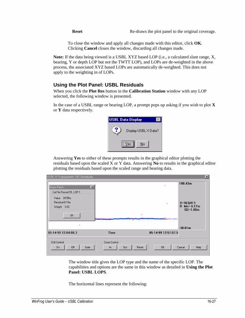
Using the Plot Panel: USBL Residuals
When you click the Plot Res button in the Calibration Station window with any LOP
selected, the following window is presented.
In the case of a USBL range or bearing LOP, a prompt pops up asking if you wish to plot X
or Y data respectively.
Answering Yes to either of these prompts results in the graphical editor plotting the
residuals based upon the scaled X or Y data. Answering No to results in the graphical editor
plotting the residuals based upon the scaled range and bearing data.
The window title gives the LOP type and the name of the specific LOP. The
capabilities and options are the same in this window as detailed in Using the Plot
Panel: USBL LOPS.
The horizontal lines represent the following:
16-28 WinFrog User’s Guide – USBL Calibration
• Long dashed magenta line is 0.
• Short dashed magenta line is the mean of all the residuals.
• Short dashed light blue line is the mean residual ± standard deviation.
The residuals are plotted against time, that is the time stamp for the data reception.
Data weighted in the solution is plotted in blue, that de-weighted is plotted in red.
Note: Though the graphically editing of Residuals is useful, it must be done carefully and
always after the initial calibration processing. It is important to be aware that the least
squares technique minimizes the residuals of all observations. Consequently, it distributes
any errors throughout the whole array. The error from a single observation will appear in
the residuals of all the observations. The amount that appears in each observation depends
upon the geometry, number of observations, and the weight assigned to each observation.
One cannot assume that the observation with the largest residual is necessarily the
observation with the error (although this is where one generally begins to investigate).
Consequently, do not eliminate large blocks of observations all at one time. Remove only a
few of the largest then solve again.
Note: If the residuals being viewed are based upon a USBL XYZ based LOP (i.e., a
calculated slant range, X, bearing, Y or depth LOP but not the TWTT LOP), and LOPs are
de-weighted in the above process, the associated XYZ based LOPs are automatically de-
weighted. This does not apply to the weighting in of LOPs.
USBL Calibration Processing The solution of the USBL calibration is a two-step process. The first step is to determine the
position of the beacon used. The second step is to use this known beacon to determine the
USBL calibration correction values. This process can be repeated to confirm the results.
However, it is recommended that the cycle not be repeated more than twice as this has a
tendency to bias the results and the solution of the calibration corrections may diverge from the
correct results.
Each step of the process has different data requirements and, as a result, the editing of the data
is approached differently for each.
The following sections detail the two steps.
Transponder Position Calibration
As mentioned, the USBL calibration requires that the position of the beacon used be
determined.
Note: the USBL range and USBL Angles (bearing LOPs) can both be used for the
determination of the beacon position (at present, the depth LOP is available only as an editing
tool, not an observable for the solution of the beacon position). However, it is recommended
that only the range LOPs be used. Experience has shown that the slope range, as extracted from
the XYZ data, is more reliable than the range and bearing for many USBL systems. More
importantly, with the use of the range LOPs only, the effects of any unapplied USBL
corrections are minimal and appear to the least squares solution as noise. If a good data
collection pattern has been employed (i.e. either the triangle or cardinal points patterns), this
noise has a minimal affect on the solution of the position as it tends to be cancelled out.
WinFrog User’s Guide – USBL Calibration 16-29
Note: the USBL range data used to calibrate a beacon position can either be that calculated
from the XYZ data or that calculated from the travel time, but not both. In the case of the latter,
a Working Velocity file must be present.
Data Editing
The editing of the data requires an initial editing prior to performing any position calculations.
This is followed by a review of the data once the first position solution has been successfully
performed, to refine the selection of valid data.
Pre-Position Solution Editing
Using the Plot Data option, as detailed previously in the USBL Calibration Data Editing
section, the POSITION and USBL range LOPs collected for the calibration should be reviewed
specifically for those points that appear to break a trend or are obvious outliers. These changes
may be exaggerated, as in the case of a bad hit on the beacon, resulting in a jump in the range to
the beacon of many meters. They may also be subtle, as in the case of the GPS losing the
differential corrections and beginning to drift from a DGPS solution.
It is equally important to re-weight into the solution those points that for one reason or another
were automatically de-weighted during the data collection process, but in review appear to be
valid.
It is important to remember that at this point, the USBL corrections are “unaccounted for.” This
may cause good data to appear to break a trend, especially in the case of the bearing and depth
LOPs. It is for this reason that these LOPs are not examined at this stage in the processing.
The graphical editor should be used to its full capability to zoom in on questionable areas of the
data. If there is doubt as to whether the data are indeed breaking a trend, do not de-weight it at
this stage.
Post-Position Solution Editing
Once a position has been solved for, the data should be reviewed again. The graphical editors
are the best editing tools to use.
It is important to remember that, at this point, the USBL corrections are still “unaccounted for.”
Review the data using the Plot Data to ensure no outliers or trend breakers were missed. Then
use the Plot Residual option to view the residuals for the POSITION and range LOPs. At this
stage, the residuals should be fairly consistent, in that they are not excessive, though in the case
of the USBL LOPs, they will probably be offset from zero. The standard deviation will
generally indicate the range of the errors due to the unaccounted for USBL corrections. Remove
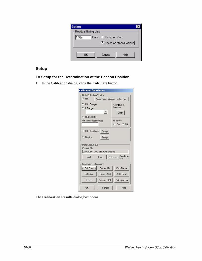
those points with large residuals. Depending upon the quality of the data, the gating feature may
be used to apply further editing of the data, although very carefully. If used, it should be applied
to the Mean Residual, not Zero, as illustrated in the following figure.
16-30 WinFrog User’s Guide – USBL Calibration
Setup
To Setup for the Determination of the Beacon Position
1 In the Calibration dialog, click the Calculate button.
The Calibration Results dialog box opens.
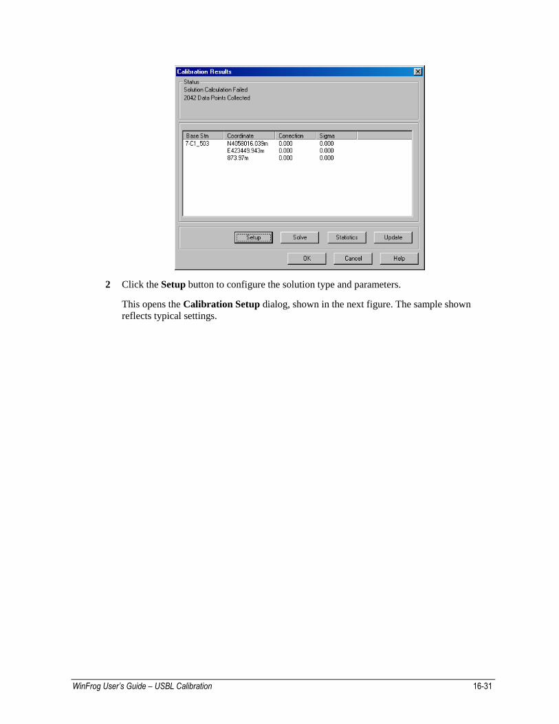
WinFrog User’s Guide – USBL Calibration 16-31
2 Click the Setup button to configure the solution type and parameters.
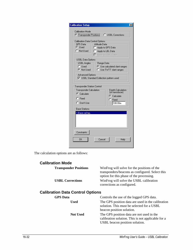
This opens the Calibration Setup dialog, shown in the next figure. The sample shown
reflects typical settings.
16-32 WinFrog User’s Guide – USBL Calibration
The calculation options are as follows:
Calibration Mode
Transponder Positions WinFrog will solve for the positions of the
transponders/beacons as configured. Select this
option for this phase of the processing.
USBL Corrections WinFrog will solve the USBL calibration
corrections as configured.
Calibration Data Control Options
GPS Data Controls the use of the logged GPS data.
Used The GPS position data are used in the calibration
solution. This must be selected for a USBL
beacon position solution.
Not Used The GPS position data are not used in the
calibration solution. This is not applicable for a
USBL beacon position solution.
WinFrog User’s Guide – USBL Calibration 16-33
Attitude Data
Apply to GPS
Data If available during the data collection, the pitch
and roll data logged with the GPS LOPs are
applied to the GPS sensor offsets in the solution.
Apply to LBL
Data Not applicable to a USBL beacon position
solution.
Apply to USBL
Data If available during the data collection, the pitch
and roll data logged with the USBL TWTT LOP
are applied to the USBL sensor offsets in the
solution. Note that this is applicable to the
transponder position portion of the calibration
process when TWTT data is used and never for
the actual USBL correction portion of the
calibration process.
USBL Angles This allows the use of USBL bearing LOPs to be
used in the solution of a USBL beacon position.
For the determination of a USBL beacon
position for the purpose of then solving the
USBL corrections, this is not to be used.
However, it is a useful tool if the position of a
beacon is required and data from a calibrated
USBL system are used to collect data without
actually circling the beacon.
Range Data Note: The radio button labels change depending
upon the data recorded.
Use calculated
slant ranges Select this option if the slant range data to be
used for the transponder beacon position
determination is derived from the XYZ data
(typical).
Use TWTT
slant ranges Select this option if the slant range data to be
used for the transponder beacon position
determination is derived from the observed
signal travel time. Note that if this option is
selected, the Attitude Data option Use Apply to
USBL Data becomes available. This is because
the travel time data is not corrected to a vertical
datum and therefore the application of pitch and
roll to the application of the sensor offsets can
improve the solution. This will be disabled if the
data does not contain two way travel time.
Use Travel Time This radio button will be present if the data
contains two way travel time with no XYZ data.
This is the case with Sonardyne’s surveyor’s
acoustic CSV telegram. When this button is
present the other two will not be present.
16-34 WinFrog User’s Guide – USBL Calibration
Advanced Options
USBL Xponder
Standard Cal This is an important setting. A standard
calibration is considered to be one that
specifically meets the objective of the design of
the data collection pattern.
To summarize the objective here, this is a
collection pattern that evenly distributes the
collection points about the beacon while
presenting the hydrophone to the beacon such
that observations fore and aft, port and starboard
are equal. If the triangle or cardinal points
pattern is used, this should be checked (default
setting). If any other pattern is used, this should
be unchecked in order to ensure that any non-
symmetry of the pattern does not bias the results.
In a Standard Cal, the vessel’s position is
considered an observation and is adjusted using
the data collected during the least squares
adjustment. In a non-Standard Cal, the vessel’s
position is considered a known and is held
unaltered during the processing from the original
position logged during the data collection.
Note: If processed as Standard Cal, in order to
revert back to the original data to try processing
as a non-Standard Cal, use the Reset USBL
option in the main Calibration dialog (see Using
the Reset USBL Option) Alternatively, reload
the original data and repeat the processing as a
non-Standard Cal.
Note: if the data were collected with the USBL
HYDROPHONE data item configuration set to
Positioning-Primary, it is recommended that
the data be processed as a standard calibration.
This is due to the real-time positioning of the
vessel having been affected by the positioning
from an uncalibrated beacon and, therefore,
must be adjusted during the processing.
Transponder Station Control
Transponder Calculation This controls the horizontal position solution for
the beacon selected in the Base Stations list
box.
Calculate Solves for the Northing and Easting of the
beacon.
Fixed The beacon is held fixed (known) in the
solution. This is not applicable in the processing
of a USBL beacon for the purpose of performing
a USBL calibration.
WinFrog User’s Guide – USBL Calibration 16-35
Don’t Use The beacon is not used at all in the solution. It is
important that if a transponder appears in the
list, but there are no data for it in the calibration
data, this option is selected for that transponder.
Otherwise, the solution will fail.
Depth Calculation
This is an important setting in any calibration, but especially in the case of a USBL
calibration. The errors solved for in the USBL calibration include a scale factor, which
(even if excessive) is largely accounted for in the least squares solution with respect to the
horizontal position determination. It can however, influence the determination of the depth,
which will subsequently greatly impact the solution of the USBL corrections. If at all
possible, the depth of the beacon should be determined using a depth sensor in the actual
beacon and then held fixed for processing. As a check, once calibrated, the same data can
be used to solve for the depth to confirm the validity of the solution.
Note: Do not confuse the term Fixed as discussed here in the context of the data processing
with the term Fixed in the configuration the actual USBL system itself. They are
completely different aspects of the calibration process. You are reminded here that the
USBL system itself must not be configured to use Fixed Depth or Telemetered Depth or
similar during the collection of calibration data.
Calculate Solves for the depth of the beacon.
Fixed The depth for the beacon is held fixed in the
solution. You may enter a value here to use as
the fixed depth. The default is the value present
in the Working Xponder file when the
calibration is first started or the depth solved in
subsequent processing.
Base Stations
This lists all the stations available for the calibration solution (set to USBL Fixed in the
Xponder file at the start of the calibration setup process or edited with the Calibration
Edit Xponder option) by station name and, if it has been entered at some point (e.g. if the
beacon is a dual purpose Sonardyne Compatt), the transponder’s address. It is important to
note that when the Calibration dialog is first opened, the current Working Xponder file is
copied to a calibration local copy of that file. It is this copy that is used throughout the
calibration process, not the actual Working Xponder file. It is for this reason that it is very
important to ensure that the Xponder file contains all transponders involved in the
calibration and has their approximate starting coordinates entered prior to starting the
calibration data collection, editing, and calculation process. If there are problems, the
calibration data set station information can be edited using the Edit Xponder feature.
Select each transponder and configure appropriately using the options available in this
panel. Once the configuration is complete, use the OK button to exit this dialog.
Additional Controls
Constraints Click this button to configure constraints for the
Least Squares Adjustment (see To Enter
Constraints for the Least Squares Adjustment).
16-36 WinFrog User’s Guide – USBL Calibration
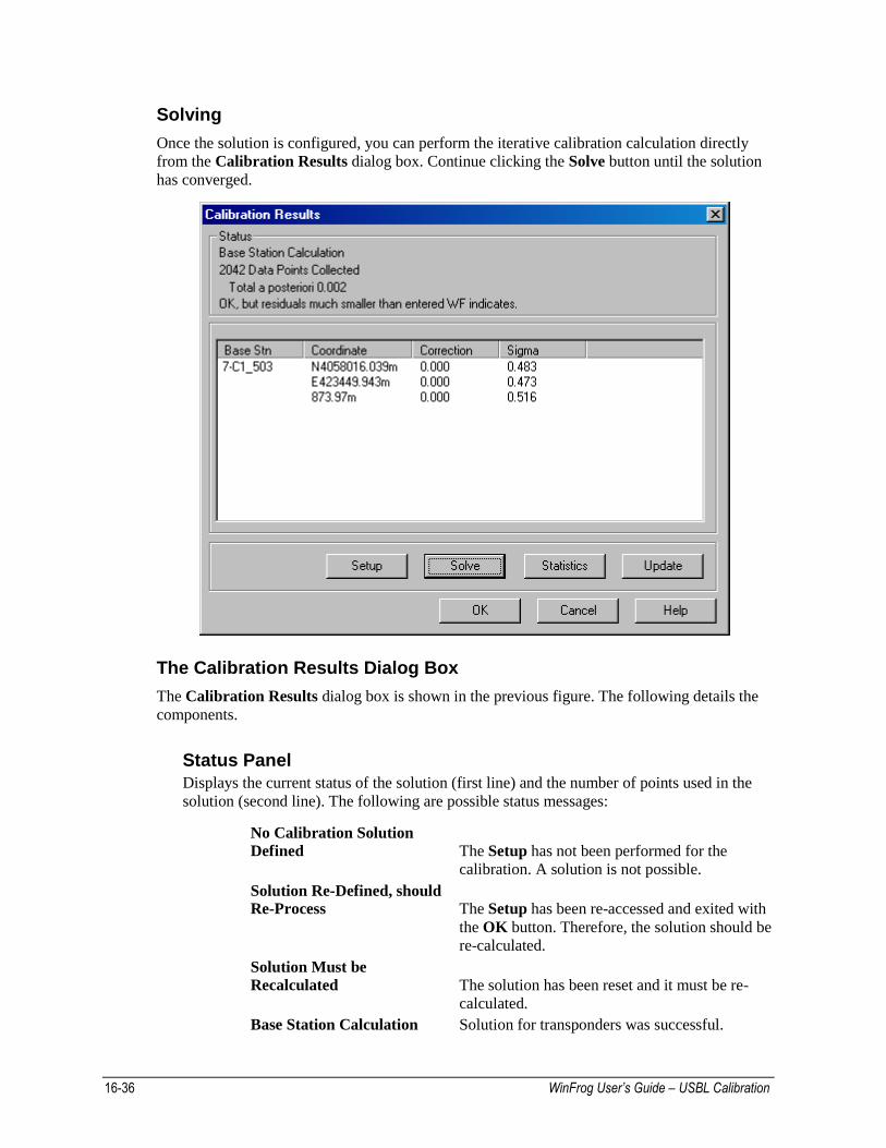
Solving
Once the solution is configured, you can perform the iterative calibration calculation directly
from the Calibration Results dialog box. Continue clicking the Solve button until the solution
has converged.
The Calibration Results Dialog Box
The Calibration Results dialog box is shown in the previous figure. The following details the
components.
Status Panel
Displays the current status of the solution (first line) and the number of points used in the
solution (second line). The following are possible status messages:
No Calibration Solution
Defined The Setup has not been performed for the
calibration. A solution is not possible.
Solution Re-Defined, should
Re-Process The Setup has been re-accessed and exited with
the OK button. Therefore, the solution should be
re-calculated.
Solution Must be
Recalculated The solution has been reset and it must be re-
calculated.
Base Station Calculation Solution for transponders was successful.
WinFrog User’s Guide – USBL Calibration 16-37
Solution Calculation Failed Solution failed. There are major problems with
the data that must be investigated.
Processing… WinFrog is executing the calibration processing.
Data Panel
Base Stn The USBL beacon name of the station.
Coordinates The Northing, Easting, and depth for the station.
Note: the Units/Coordinates/Grid Coordinate
Order controls the order of the Northing or
Easting.
Corrections The corrections determined and applied in the
last adjustment iteration. If the associated
coordinate component has been held Fixed,
instead of the correction value, the term Fixed is
displayed in brackets.
Note: the term corrections here refers to the
adjustments to the unknowns determined by the
least squares adjustment, not the USBL
corrections. The unknowns in this processing are
the beacon coordinates and depth, if it is to be
solved.
Sigmas The sigma of the associated coordinate
component as determined from the last
adjustment iteration.
To Perform the Adjustment
As mentioned previously, the least squares solution is an iterative one.
1 Click the Solve button to perform one adjustment. If the solution is successful (converges),
the results of the adjustment are displayed.
2 Continue to click the Solve button until the value no longer changes with each click.
The correction values continue to converge (get smaller), eventually reaching a value that
remains unchanged on subsequent clicks of the Solve button. This indicates that the
calibration adjustment is complete based upon the currently weighted data.
Note: in a “perfect” solution, the correction values would converge to zero. However, in the
actual calibration, they should converge to values consistent with the accuracy of the
acoustic system being used.
Problems with the calibration data are indicated by the following:
The solution fails. Probable causes are:
A transponder has no data associated with it, but is not set to Don’t Use.
The initial transponder coordinates and/or depths are not sufficiently close to the
actual locations. Also, check that the correct transponder was dropped or located
at the correct location.
There are flyers that have not been de-weighted from the solution.
Incorrect beacons in file. To correct:
A - Exit the calibration process
16-38 WinFrog User’s Guide – USBL Calibration
B - Confirm the validity and completeness of the Working Xponder file
C - Start a new calibration
D - Save to a dummy file.
E - Use a text editor to replace the 901 records in the real calibration file with
those in the just created dummy file.
GPS Data is set to Not Used
The correction values converge, but not to a value consistent with the accuracy
capabilities of the acoustic system being calibrated. This indicates that there are
probably still bad data weighted in the solution. The LOPs should be re-
examined using the graphical editor.
The correction values jump about without converging, or appear to converge,
but before reaching a static result start to increase again. This again indicates
that there are probably still bad data weighted in the solution. The LOPs should
be re-examined using the graphical editor.
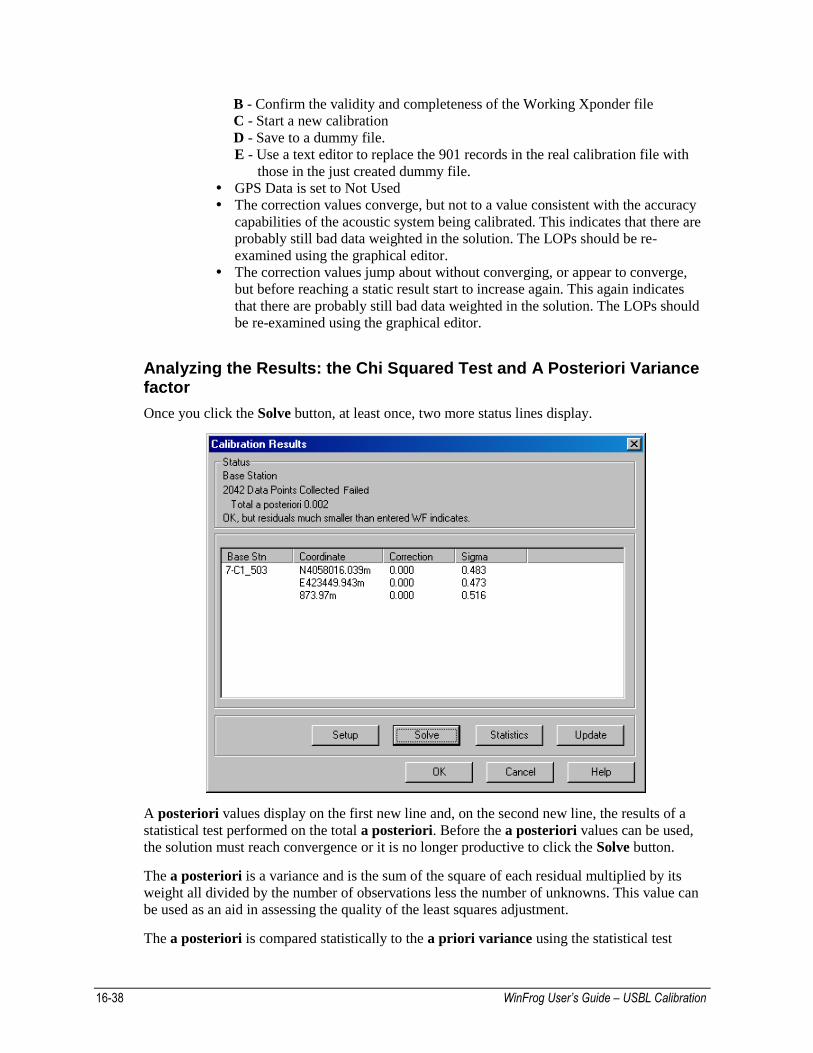
Analyzing the Results: the Chi Squared Test and A Posteriori Variance factor
Once you click the Solve button, at least once, two more status lines display.
A posteriori values display on the first new line and, on the second new line, the results of a
statistical test performed on the total a posteriori. Before the a posteriori values can be used,
the solution must reach convergence or it is no longer productive to click the Solve button.
The a posteriori is a variance and is the sum of the square of each residual multiplied by its
weight all divided by the number of observations less the number of unknowns. This value can
be used as an aid in assessing the quality of the least squares adjustment.
The a posteriori is compared statistically to the a priori variance using the statistical test
WinFrog User’s Guide – USBL Calibration 16-39
termed the Chi squared test. This test is performed at a 95% confidence interval. The value of
the a priori variance is 1 because the standard deviation of each observation is known and set
by the operator.
Why could the Chi Squared Test Fail?
If the test fails and the a posteriori variance is large, the adjustment and consequently the
calculated coordinates of the transponders are unreliable. A failure of this statistical test can
occur for three reasons:
• bad mathematical model
• unmodeled biases in the data (some bad observations)
• incorrect initial weighting (wrong Weighting Factor)
The first possible cause of the failure can be discounted as the mathematical model has been
proven sound by several authors over many years.
The second cause of the failure, unmodeled biases in the data, is usually the cause that
requires investigation. This can be due to the following:
• There is one or more bad observation: a baseline, surface-to-transponder range,
depth or GPS fix.
• Excessive pitch and roll of the vessel during recording of the transceiver-to-
transponder ranges without an attitude sensor input to WinFrog and enabled for
use in the Vehicle positioning. This could effect all surface-to-transponder ranges
and GPS positions. In this case, the unmodeled bias in the data is the un-
calculated change in range due to pitch and roll. (Actually the ship rocks so the
offset between the GPS antenna and the transponder is not correct so the
transponder coordinates are calculated incorrectly at the time the observation is
made.) WinFrog can be configured to use an attitude sensor in realtime and log
the data to the calibration data for use in the calibration processing, if an attitude
sensor is available when the data is observed.
If an attitude sensor is not available and there is excessive ship pitch and roll the
residuals will show a marked sinusoid pattern. The crests and troughs will
usually straddle the mean, but not always evenly as the ship may roll to one side
more than the other. If there are a large number of observations and all the larger
outliers are removed, the pitch or roll to one side will cancel the pitch or roll to
the other and the adjustment should be good. However in this situation one
should multiply the geometric error ellipses by the square root of the total a
posteriori variance to obtain the actual absolute error ellipses. This will then
reflect the uncertainty in the absolute accuracy of the transponders due to the un-
modeled pitch and roll.
• Invalid velocity profile.
The size of the a posteriori is a qualitative indicator of how many bad observations there are. It
usually only requires one bad observation to cause the failure. However, when this happens the
a posteriori variance is usually smaller (say less than 10). The more bad observations there are,
the larger the a posteriori variance can become. If it is greater than 999, it indicates that there
are several bad observations. Note: one large error is roughly equivalent to a few smaller errors.
The third possible reason that the test on the a posteriori variance factor can fail is incorrect
16-40 WinFrog User’s Guide – USBL Calibration
initial weighting. The initial weighting is the weighting factor value assigned to each
observation. The status line may display the message, OK, but residuals much smaller than
initial WF indicates. This means that the statistical test failed, but not due to bad data. This is
caused by assigning weighting factor values that were too pessimistic to the observations, i.e. the
standard error of each observation is better than that entered, as determined by the least squares
adjustment. In this case, the solution is still good and the coordinates are reliable.
The weighting factors can be reduced and the solution re-processed to determine if this improves
the a posteriori variances. However, it is important not to reduce them to unreasonably small
values simply to achieve satisfactory a posteriori variances. If the weighting factors are
reasonable, accept the results and use the geometric error ellipses for the absolute error ellipses
and the error ellipses estimated from the Baseline a posteriori as the bottom relative error ellipses.
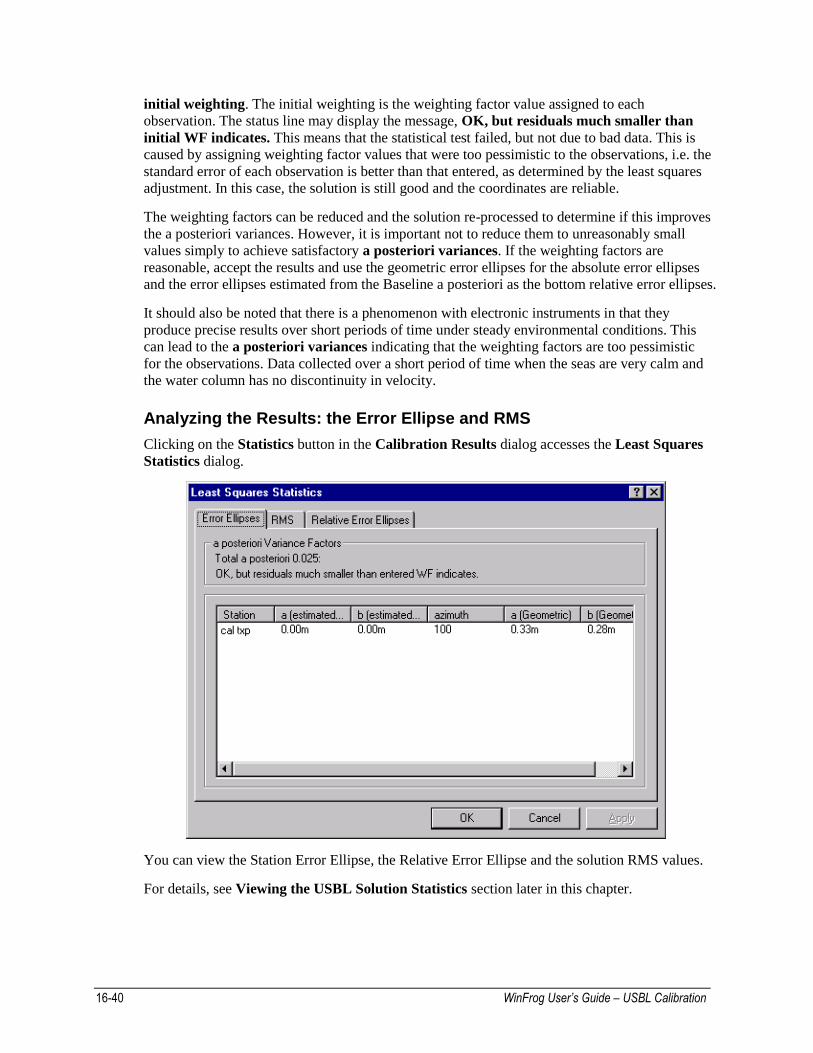
It should also be noted that there is a phenomenon with electronic instruments in that they
produce precise results over short periods of time under steady environmental conditions. This
can lead to the a posteriori variances indicating that the weighting factors are too pessimistic
for the observations. Data collected over a short period of time when the seas are very calm and
the water column has no discontinuity in velocity.
Analyzing the Results: the Error Ellipse and RMS
Clicking on the Statistics button in the Calibration Results dialog accesses the Least Squares
Statistics dialog.
You can view the Station Error Ellipse, the Relative Error Ellipse and the solution RMS values.
For details, see Viewing the USBL Solution Statistics section later in this chapter.
WinFrog User’s Guide – USBL Calibration 16-41
Examining the Results and Repeating the Process
The process of reviewing and editing the data and then performing an adjustment should be
repeated several times. The actual number of cycles depends upon the quality of the data. The
objective is to achieve a reliable solution while using most of the data.
When editing the data by looking at the residuals, be aware that the least squares technique
minimizes the residuals of all of the observations. Consequently, it distributes any errors
throughout the whole array. The error from a single observation will appear in the residuals of
all observations. The amount that appears in each observation depends upon the geometry,
number of observations, and the weight assigned to each observation. One cannot assume that
the observation with the largest residual is necessarily the observation with the error (although
this is where one generally begins to investigate). Therefore, do not eliminate large blocks of
observations all at one time. Remove only a few of the largest, then solve again.
In addition, the USBL corrections are still un-accounted for and the residuals may not be
centered around 0 as one might expect. In this stage, only those LOPs whose residuals are
extreme and are obviously outside of the main grouping should be de-weighted.
Note: as previously mentioned, it is recommended that the calibration be saved after each cycle.
In this way, you can return to a known point or resume processing at a later time, if required.
Once the calibration is considered complete and the final calibration file is saved to a new file,
the intermediate files can be removed, leaving the original untouched file and the final result
file. By loading the final result file, the calibration can be reviewed and/or printed at any time
without having to perform any step other than loading the file.
Note: when a calibration file is saved, all configuration settings are also saved.
Note: if the USBL calibration is being performed only to calibrate the position of USBL
beacons, then the processing is completed after repeating the process as detailed above. A report
can then be generated.
USBL Calibration
With a known beacon position, the USBL system corrections can be determined. This process
requires the same steps as followed for determining the beacon position.
Data Editing
Similar to the editing of the data for the position determination, the editing of the data for the
actual USBL corrections determination has a pre-first solution and post-first solution aspect to
it.
In both cases, the data editing now focuses on the USBL data, specifically the bearing and depth
LOPs. Whereas the range LOP is the least affected of the USBL LOPs by the corrections to be
solved for (and thus the LOP to examine and use for the beacon position solution), the bearing
and depth LOPs are greatly affected. Therefore, they are better indicators of the validity of the
USBL data for use in the determination of the corrections and the results of subsequent
correction determinations. The bearing can also be examined as the X and Y data (see Using
the Plot Panel: USBL LOPs).
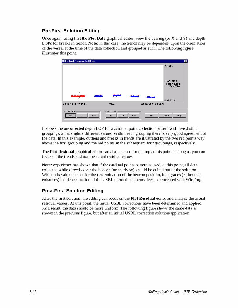
16-42 WinFrog User’s Guide – USBL Calibration
Pre-First Solution Editing
Once again, using first the Plot Data graphical editor, view the bearing (or X and Y) and depth
LOPs for breaks in trends. Note: in this case, the trends may be dependent upon the orientation
of the vessel at the time of the data collection and grouped as such. The following figure
illustrates this point.
It shows the uncorrected depth LOP for a cardinal point collection pattern with five distinct
groupings, all at slightly different values. Within each grouping there is very good agreement of
the data. In this example, outliers and breaks in trends are illustrated by the two red points way
above the first grouping and the red points in the subsequent four groupings, respectively.
The Plot Residual graphical editor can also be used for editing at this point, as long as you can
focus on the trends and not the actual residual values.
Note: experience has shown that if the cardinal points pattern is used, at this point, all data
collected while directly over the beacon (or nearly so) should be edited out of the solution.
While it is valuable data for the determination of the beacon position, it degrades (rather than
enhances) the determination of the USBL corrections themselves as processed with WinFrog.
Post-First Solution Editing
After the first solution, the editing can focus on the Plot Residual editor and analyze the actual
residual values. At this point, the initial USBL corrections have been determined and applied.
As a result, the data should be more uniform. The following figure shows the same data as
shown in the previous figure, but after an initial USBL correction solution/application.
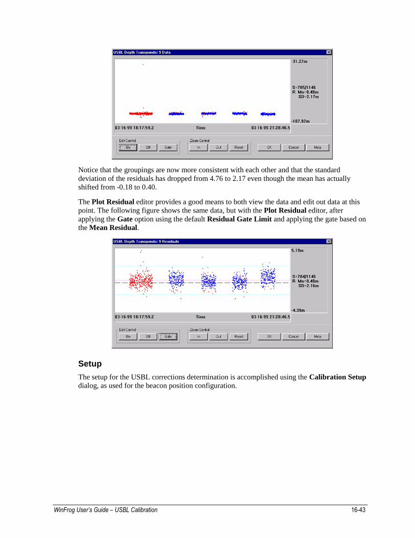
WinFrog User’s Guide – USBL Calibration 16-43
Notice that the groupings are now more consistent with each other and that the standard
deviation of the residuals has dropped from 4.76 to 2.17 even though the mean has actually
shifted from -0.18 to 0.40.
The Plot Residual editor provides a good means to both view the data and edit out data at this
point. The following figure shows the same data, but with the Plot Residual editor, after
applying the Gate option using the default Residual Gate Limit and applying the gate based on
the Mean Residual.
Setup
The setup for the USBL corrections determination is accomplished using the Calibration Setup
dialog, as used for the beacon position configuration.
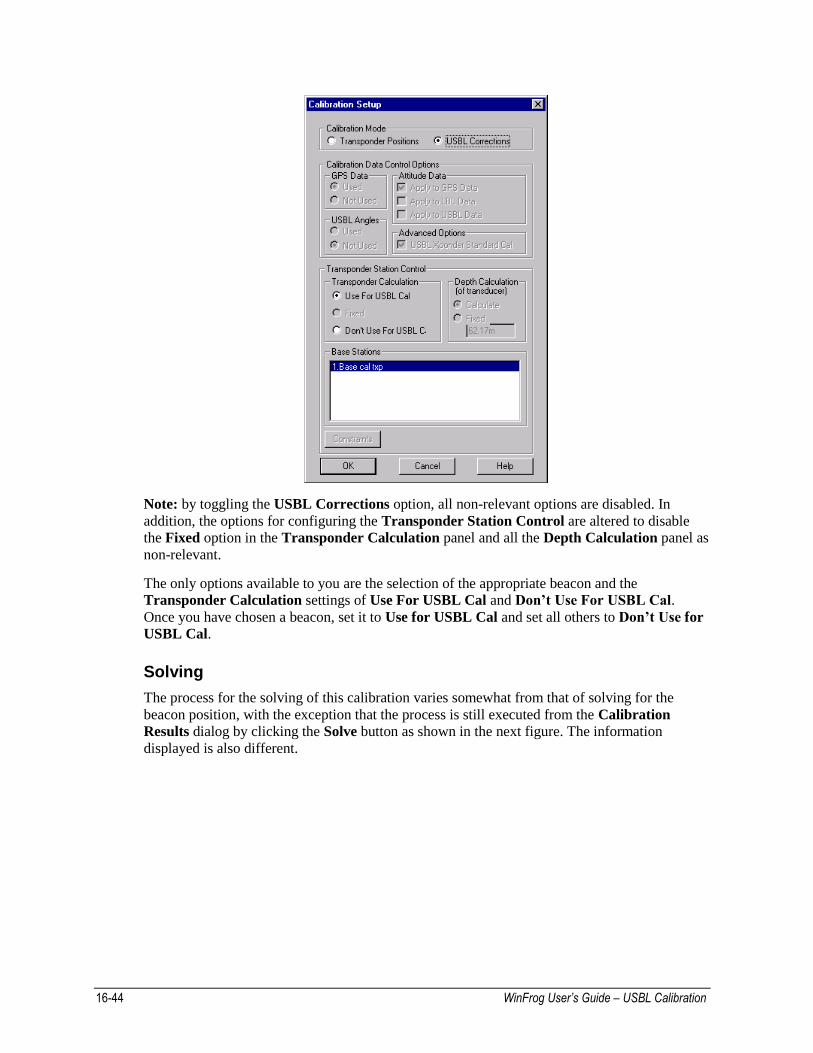
16-44 WinFrog User’s Guide – USBL Calibration
Note: by toggling the USBL Corrections option, all non-relevant options are disabled. In
addition, the options for configuring the Transponder Station Control are altered to disable
the Fixed option in the Transponder Calculation panel and all the Depth Calculation panel as
non-relevant.
The only options available to you are the selection of the appropriate beacon and the
Transponder Calculation settings of Use For USBL Cal and Don’t Use For USBL Cal.
Once you have chosen a beacon, set it to Use for USBL Cal and set all others to Don’t Use for
USBL Cal.
Solving
The process for the solving of this calibration varies somewhat from that of solving for the
beacon position, with the exception that the process is still executed from the Calibration
Results dialog by clicking the Solve button as shown in the next figure. The information
displayed is also different.
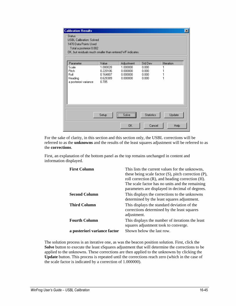
WinFrog User’s Guide – USBL Calibration 16-45
For the sake of clarity, in this section and this section only, the USBL corrections will be
referred to as the unknowns and the results of the least squares adjustment will be referred to as
the corrections.
First, an explanation of the bottom panel as the top remains unchanged in content and
information displayed.
First Column This lists the current values for the unknowns,
these being scale factor (S), pitch correction (P),
roll correction (R), and heading correction (H).
The scale factor has no units and the remaining
parameters are displayed in decimal of degrees.
Second Column This displays the corrections to the unknowns
determined by the least squares adjustment.
Third Column This displays the standard deviation of the
corrections determined by the least squares
adjustment.
Fourth Column This displays the number of iterations the least
squares adjustment took to converge.
a posteriori variance factor Shown below the last row.
The solution process is an iterative one, as was the beacon position solution. First, click the
Solve button to execute the least sSquares adjustment that will determine the corrections to be
applied to the unknowns. These corrections are then applied to the unknowns by clicking the
Update button. This process is repeated until the corrections reach zero (which in the case of
the scale factor is indicated by a correction of 1.000000).
16-46 WinFrog User’s Guide – USBL Calibration
If the solution does not converge to zero, there is either insufficient data or there are bad points
present in the weighted-in data. If this occurs, the data must be reviewed using the editors to
determine the cause of the problem.
Analysis of the Results and Repeating
The results themselves are the primary tools for analysis. These provide a graphic presentation
of the result of the determination of not just the beacon position, but of the data after
determination and application of the USBL corrections. The a posteriori variance factor is also
an indication of the quality of the data and the results. (Another important tool is the USBL
Calibration Report, which will be discussed in a subsequent section.)
After completing a Solve/Update cycle, the data should be reviewed using the Plot Residual
editor. Now that the USBL corrections have been determined and applied, the residuals should
be reduced and match the expected accuracy of the systems involved. In addition, they should
now be centered about or close to zero rather than offset, as is the case prior to this step. The
Gate option can now be used to refine the data to be included in the calibration.
Unfortunately, there are no specific quantitative measures to compare the data against, to decide
what data are acceptable and what data are to be removed. The data must be viewed by
comparing any one LOP to the whole data set.
The prevailing environmental conditions at the time the data were collected have a very large
impact on the results.
Another, but less reliable, analysis tool is the a posteriori variance factor. This should be equal
to one (1.0). A value (much) lower than one is possible when a large quantity of data of high
quality has been collected and/or the weights used are relatively high and pessimistic. A value
greater than one does not necessarily indicate a bad solution, though if this value is greater than
10 the data should be reviewed for outliers.
It is recommended that the data be reviewed and edited once and then the Solve/Update cycle
repeated again afterwards.
As a confirmation, the beacon position can be resolved for using the now corrected data. If the
editing and processing have been correctly performed, the change in the position will be in the
centimeter to decimeter range. If the change is greater, the solution must be suspect and
restarted with greater attention paid to editing the data.
Note: it is recommended that the process of solving the beacon position after the determination
of the USBL corrections be performed for the purpose of confirming the results of the whole
USBL Calibration process only. Repeating the solution of the USBL corrections after resolving
the beacon position can lead to a never-ending cycle that can actually cause the results to
diverge from the correct results.
Viewing the USBL Solution Statistics When a least squares adjustment of the station coordinates is performed the variance co-
variance matrix of all the stations is also computed. These values are independent of the
observations. They are dependent upon geometry and the weighting factors assigned to each
observation.
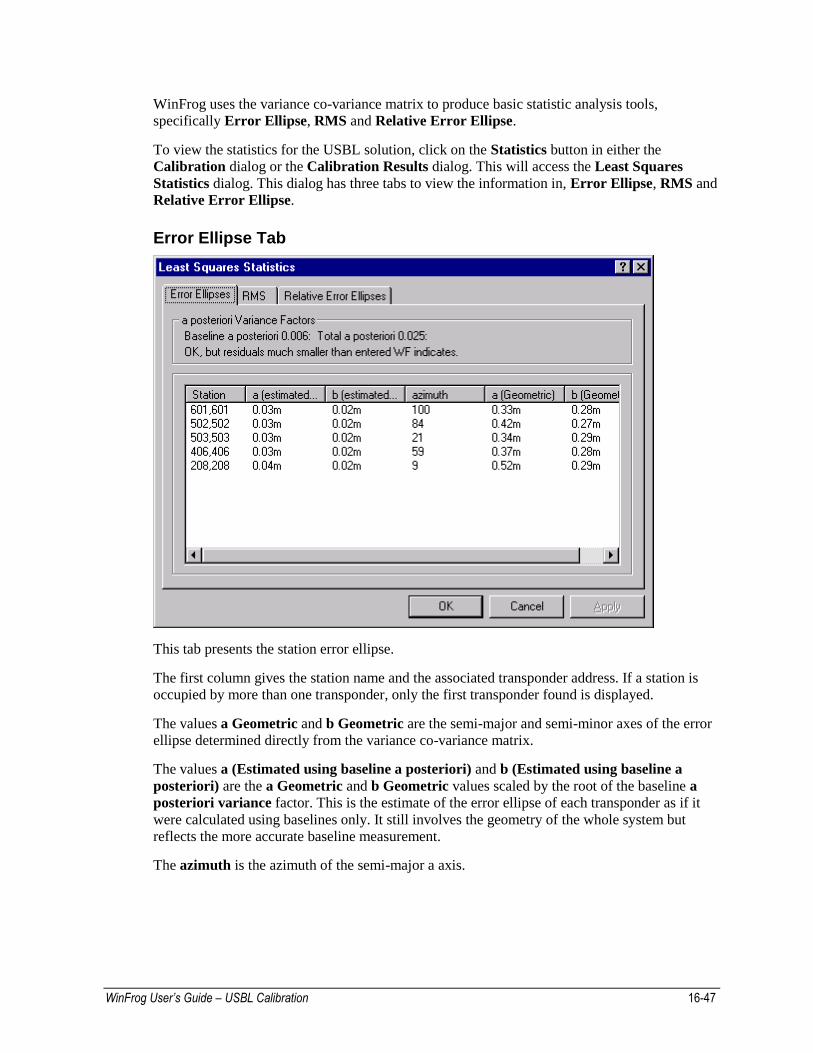
WinFrog User’s Guide – USBL Calibration 16-47
WinFrog uses the variance co-variance matrix to produce basic statistic analysis tools,
specifically Error Ellipse, RMS and Relative Error Ellipse.
To view the statistics for the USBL solution, click on the Statistics button in either the
Calibration dialog or the Calibration Results dialog. This will access the Least Squares
Statistics dialog. This dialog has three tabs to view the information in, Error Ellipse, RMS and
Relative Error Ellipse.
Error Ellipse Tab
This tab presents the station error ellipse.
The first column gives the station name and the associated transponder address. If a station is
occupied by more than one transponder, only the first transponder found is displayed.
The values a Geometric and b Geometric are the semi-major and semi-minor axes of the error
ellipse determined directly from the variance co-variance matrix.
The values a (Estimated using baseline a posteriori) and b (Estimated using baseline a
posteriori) are the a Geometric and b Geometric values scaled by the root of the baseline a
posteriori variance factor. This is the estimate of the error ellipse of each transponder as if it
were calculated using baselines only. It still involves the geometry of the whole system but
reflects the more accurate baseline measurement.
The azimuth is the azimuth of the semi-major a axis.
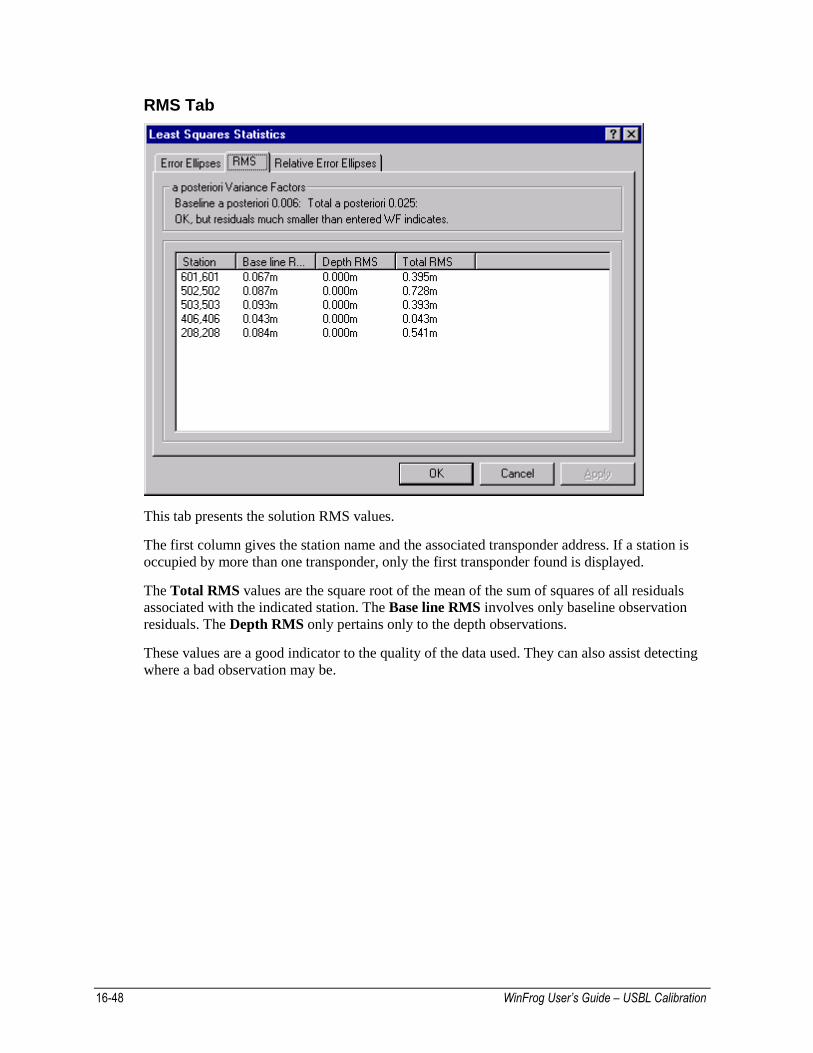
16-48 WinFrog User’s Guide – USBL Calibration
RMS Tab
This tab presents the solution RMS values.
The first column gives the station name and the associated transponder address. If a station is
occupied by more than one transponder, only the first transponder found is displayed.
The Total RMS values are the square root of the mean of the sum of squares of all residuals
associated with the indicated station. The Base line RMS involves only baseline observation
residuals. The Depth RMS only pertains only to the depth observations.
These values are a good indicator to the quality of the data used. They can also assist detecting
where a bad observation may be.
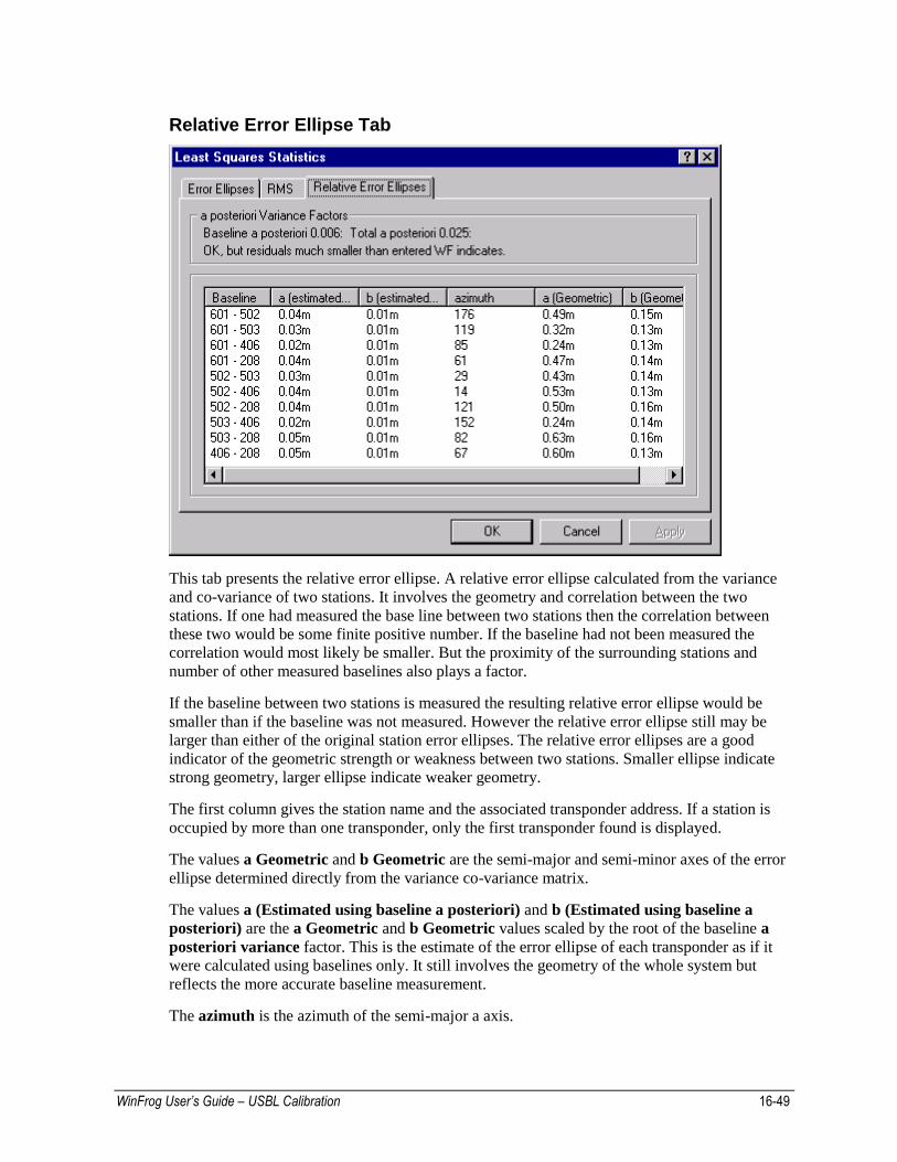
WinFrog User’s Guide – USBL Calibration 16-49
Relative Error Ellipse Tab
This tab presents the relative error ellipse. A relative error ellipse calculated from the variance
and co-variance of two stations. It involves the geometry and correlation between the two
stations. If one had measured the base line between two stations then the correlation between
these two would be some finite positive number. If the baseline had not been measured the
correlation would most likely be smaller. But the proximity of the surrounding stations and
number of other measured baselines also plays a factor.
If the baseline between two stations is measured the resulting relative error ellipse would be
smaller than if the baseline was not measured. However the relative error ellipse still may be
larger than either of the original station error ellipses. The relative error ellipses are a good
indicator of the geometric strength or weakness between two stations. Smaller ellipse indicate
strong geometry, larger ellipse indicate weaker geometry.
The first column gives the station name and the associated transponder address. If a station is
occupied by more than one transponder, only the first transponder found is displayed.
The values a Geometric and b Geometric are the semi-major and semi-minor axes of the error
ellipse determined directly from the variance co-variance matrix.
The values a (Estimated using baseline a posteriori) and b (Estimated using baseline a
posteriori) are the a Geometric and b Geometric values scaled by the root of the baseline a
posteriori variance factor. This is the estimate of the error ellipse of each transponder as if it
were calculated using baselines only. It still involves the geometry of the whole system but
reflects the more accurate baseline measurement.
The azimuth is the azimuth of the semi-major a axis.
16-50 WinFrog User’s Guide – USBL Calibration
USBL Calibration Reporting Reporting for the USBL Calibration is accessed from the Acoustic Calibration dialog by
clicking the USBL Report button. The results of the calibration are printed along with some
statistical values and graphs described below.
The data presented in the USBL calibration report is described below and is essentially derived
by comparison of raw USBL data to the mean position derived from that raw data and
comparison of corrected USBL data to the mean position derived from that corrected data.
The maximum and minimum values of each set are displayed along with a mean, standard
deviation and root mean square (RMS). The main values to consider when assessing the
calibration are the Range C-O of the corrected data, specifically the mean. This is because it’s
the range that is used as the observation for the calibration.
The other C-O quantities are derived, but their RMS should provide a better evaluation number
than the standard deviation. See below for a description of each.
Transponder Coordinates Summary of the results of the position
determination of the beacon used for the
calibration, specifically:
· the beacon code;
· Northing c/w standard deviation;
· Easting c/w standard deviation; and
· Depth c/w standard deviation (if solved for).
Calibration Results Summary of the results of the determination of
the USBL Corrections, specifically:
· the Scale Factor (no units),
· Pitch Correction (decimal of degrees);
· Roll Correction (decimal of degrees);
· Heading Correction (decimal of degrees);
· the a posteriori variance factor; and
· the total number of data available and used in
the calibration.
Data Summary Table The summary table presents the minimum,
maximum, mean, and standard deviation based
upon Calculated-Observed (C-O) for un-corrected
and corrected USBL data. In addition, the RMS
for the respective C-O data sets is given for the
corrected data. Note: to produce these values, the
components of each calibration data record (XYZ)
are subtracted from the corresponding calculated
values derived from the calibrated beacon position
and the USBL hydrophone position. In the case of
the beacon position, range, and azimuth
comparisons, these are derived from the XYZ data
for each calibration data record. Note that only
that data weighted in the USBL calibration
solution are used.
WinFrog User’s Guide – USBL Calibration 16-51
Psns C-O The distance between the mean beacon position
and the position derived from each observation
set (raw and corrected) is calculated. The
statistical values of these two sets are calculated
and displayed. NOTE: This data set is not
normally distributed. In a normally distributed
data set, whose expected mean is zero, adding
more data should cause the mean to approach
zero since some values will be positive and
some negative. However, the distance between
two points is always positive, thus the expected
mean is not zero. Consequently, the mean and
standard deviation should only be looked at as
an indication of the noise in the data. Larger
values indicate noisier data. The RMS is the
better quantity to look at here.
X, Y and Z C-O This is related to the vessel, X port/starboard, Y
fore/aft and Z up/down. The known transceiver
position is compared to the mean beacon
position (raw and corrected) to produce the
computed X, Y or Z value. The difference
between this value and each observed X, Y and
Z value is determined to produce the data sets.
One set for raw data and one for corrected data
for each item. This data should be normally
distributed and does give an indication of the
error in these directions.
Range C-O Similarly to above, the slant range between the
known transceiver position and the mean beacon
positions (raw and corrected) are calculated. From
that is subtracted the slant range (derived from each
USBL observation set) to produce the data sets, one
for raw and one for corrected. This data should be
normally distributed and does give an indication of
the range error. This is the observation that is used
to calculate the beacon position.
Note: Of all the USBL corrections the only one
that affects the slant range is the scalar. Since
the scalar is small there will be very little
difference between the uncorrected and
corrected data.
Bearing C-O The azimuths from the USBL transceiver to the
mean beacon positions (raw and corrected) are
calculated. From these are subtracted the
azimuth from the USBL transceiver to each
observed beacon position (raw and corrected).
This data should be normally distributed.
Perhaps somewhat abstract, these values usually
experience the greatest change between the raw
and corrected data sets.
16-52 WinFrog User’s Guide – USBL Calibration
Plots and Histograms
The histograms based upon the data calculated to produce the Data Summary Table. Note
that only that data weighted in the USBL calibration solution are used. The histograms
include the mean value drawn as a vertical line at the appropriate position complete with
annotation. The standard deviations are also drawn as vertical lines in the appropriate
position.
Vehicle Position This is a plot of the vehicle positions during the
data collection, centered about the calculated
beacon position.
Beacon Position,
Uncorrected USBL This is a scatter plot of the USBL beacon
position calculated for each epoch using un-
corrected USBL data, centered about the
calculated beacon position. Note this is always
uncorrected data. If the data was gathered with
calibration corrections already in the
Hydrophone Data Item configuration dialog they
are not applied in this plot.
Beacon Position,
Corrected USBL This is a scatter plot of the USBL beacon
position calculated for each epoch using
corrected USBL data, centered about the
calculated beacon position. Look for a tighter
group about the center than the uncorrected.
Coor. Position C-O Histogram of the distance from the solved for
USBL beacon position to the position calculated
for each epoch using corrected USBL data for
each epoch. Since the values are distances they
are always positive. This graph indicates how
noisy the data is. The more spread out the graph,
the noisier the data.
In the following histograms look for an improvement in the shape of the corrected data
histograms. The shape should represent a normal distribution.
Raw Range Res, C-O Histogram of the uncorrected USBL range
residuals.
Corr’d Range Res, C-O Histogram of the corrected USBL range
residuals.
Raw Bearing Res, C-O Histogram of the uncorrected USBL bearing
residuals.
Corr’d Bearing Res, C-O Histogram of the corrected USBL bearing
residuals.
Raw X Res, C-O Histogram of the uncorrected USBL X
component residuals.
Corr’d X Res, C-O Histogram of the corrected USBL X component
residuals.
WinFrog User’s Guide – USBL Calibration 16-53
Raw Y Res, C-O Histogram of the uncorrected USBL Y
component residuals.
Corr’d Y Res, C-O Histogram of the corrected USBL Y component
residuals.
Raw Z Res, C-O Histogram of the uncorrected USBL Z
component residuals.
Corr’d Z Res, C-O Histogram of the corrected USBL Z component
residuals.
This window is a valuable analysis tool for the USBL calibration. The scatter plots clearly
illustrate the quality of the data collected and the processing, supported by the histograms. As
an analysis tool, this report provides you with the best summary of all aspects of calibration one
place and should be utilized as such.
Clicking the right mouse button with the cursor in this window gives a pop-up menu with the
following options:
Save to a metafile
This allows you to save the window as an enhanced metafile, which can, subsequently, be
inserted into a document. The example in this manual has been created and inserted in this
way. This provides a report quality presentation of the USBL calibration suitable for
presentation to clients.
Save to CSV file
Saves the data to a file using comma-delimited fields to enable easy loading into another
software package.
Change Vehicle Pos. Scale
Allows you to manipulate the scale of the panel containing the plot of the calibration data
collection points.
Change USBL data Scale
Allows you to manipulate the scale of the panels containing the calculated beacon positions
based upon the raw and corrected USBL data. Note that both panels are plotted with the
same scale.
Change color Graphics
Allows you to manipulate the background color of all panels.
Change color Data
Allows you to manipulate the color used to plot the histogram data.
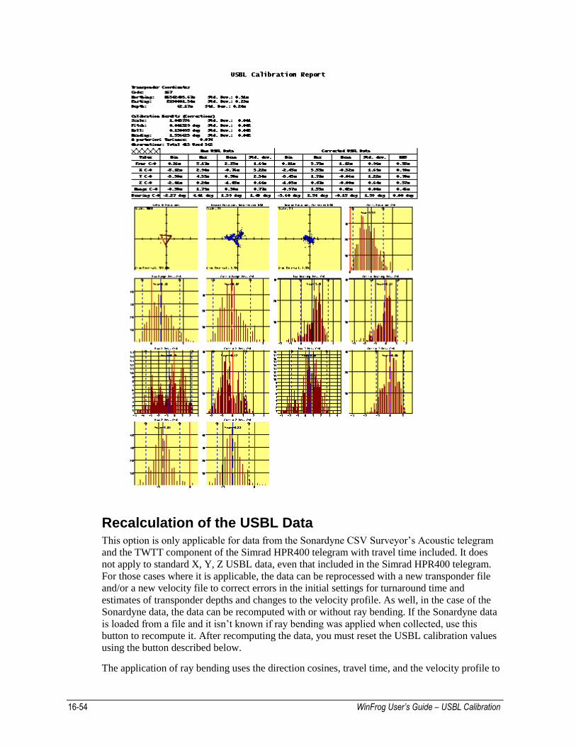
16-54 WinFrog User’s Guide – USBL Calibration
Recalculation of the USBL Data This option is only applicable for data from the Sonardyne CSV Surveyor’s Acoustic telegram
and the TWTT component of the Simrad HPR400 telegram with travel time included. It does
not apply to standard X, Y, Z USBL data, even that included in the Simrad HPR400 telegram.
For those cases where it is applicable, the data can be reprocessed with a new transponder file
and/or a new velocity file to correct errors in the initial settings for turnaround time and
estimates of transponder depths and changes to the velocity profile. As well, in the case of the
Sonardyne data, the data can be recomputed with or without ray bending. If the Sonardyne data
is loaded from a file and it isn’t known if ray bending was applied when collected, use this
button to recompute it. After recomputing the data, you must reset the USBL calibration values
using the button described below.
The application of ray bending uses the direction cosines, travel time, and the velocity profile to
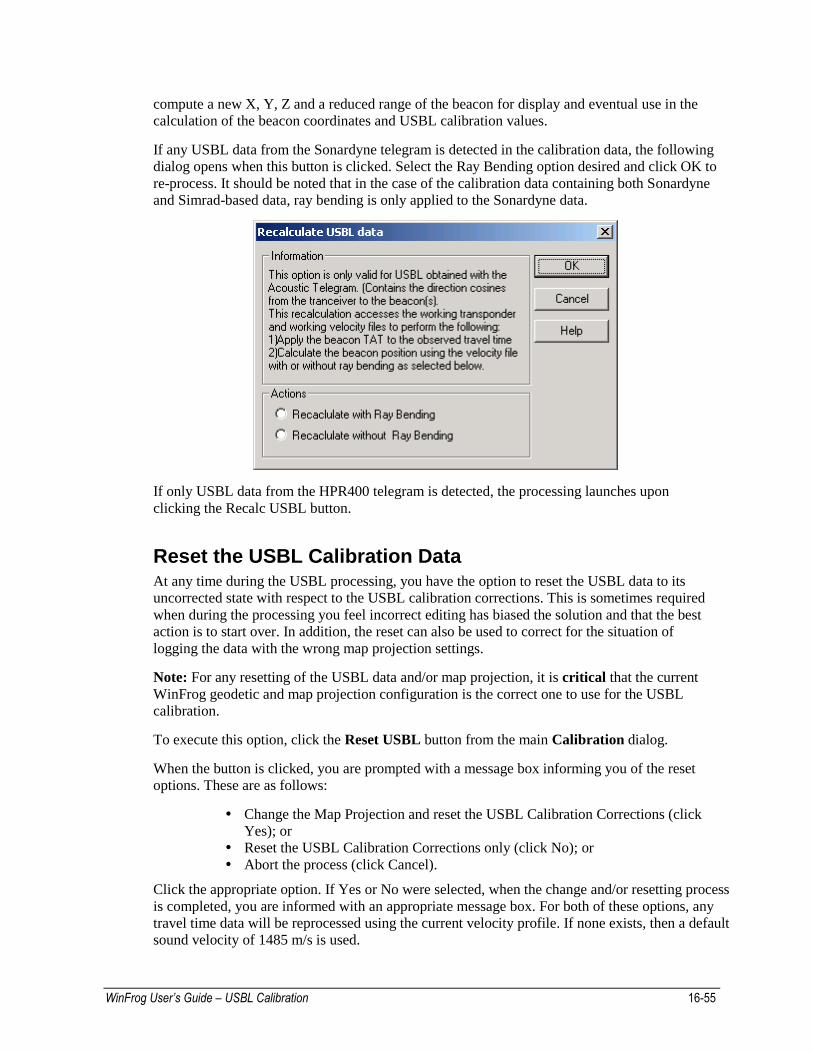
WinFrog User’s Guide – USBL Calibration 16-55
compute a new X, Y, Z and a reduced range of the beacon for display and eventual use in the
calculation of the beacon coordinates and USBL calibration values.
If any USBL data from the Sonardyne telegram is detected in the calibration data, the following
dialog opens when this button is clicked. Select the Ray Bending option desired and click OK to
re-process. It should be noted that in the case of the calibration data containing both Sonardyne
and Simrad-based data, ray bending is only applied to the Sonardyne data.
If only USBL data from the HPR400 telegram is detected, the processing launches upon
clicking the Recalc USBL button.
Reset the USBL Calibration Data At any time during the USBL processing, you have the option to reset the USBL data to its
uncorrected state with respect to the USBL calibration corrections. This is sometimes required
when during the processing you feel incorrect editing has biased the solution and that the best
action is to start over. In addition, the reset can also be used to correct for the situation of
logging the data with the wrong map projection settings.
Note: For any resetting of the USBL data and/or map projection, it is critical that the current
WinFrog geodetic and map projection configuration is the correct one to use for the USBL
calibration.
To execute this option, click the Reset USBL button from the main Calibration dialog.
When the button is clicked, you are prompted with a message box informing you of the reset
options. These are as follows:
Change the Map Projection and reset the USBL Calibration Corrections (click
Yes); or
Reset the USBL Calibration Corrections only (click No); or
Abort the process (click Cancel).
Click the appropriate option. If Yes or No were selected, when the change and/or resetting process
is completed, you are informed with an appropriate message box. For both of these options, any
travel time data will be reprocessed using the current velocity profile. If none exists, then a default
sound velocity of 1485 m/s is used.
16-56 WinFrog User’s Guide – USBL Calibration
The Transformation to a new Map Projection
The change of the map projection involves the following:
Transforms the geographic coordinates for all base stations in the calibration
data set to the current Working Map Projection.
Transforms the geographic vessel positions to the current Working Map
Projection.
Transforms the raw position LOPs (WGS84 ellipsoid latitude and longitude) to
the current Working Ellipsoid and then to the current Working Map Projection.
Note: If the working ellipsoid is NAD83, SPCS 83, SPCS 27 using the
NADCON transformation or NAD 27 using the NADCON transformation, and
the calibration data has been loaded from a file, the ITRF/NAD83
transformation parameters are calculated for each calibration data epoch. This
applies to the case of calibration data loaded from a file and then added to before
this action is executed.
The Resetting of the USBL Data
The resetting of the USBL data involves the following:
The current USBL corrections are reset to default values, that is scale = 1, pitch
= 0, roll = 0 and heading = 0.
The raw XYZ data are reprocessed with the reset calibration corrections and are
projected to the current Working Map Projection to derive new scaled LOPs.
If TWTT data are available, the current Working Velocity file is accessed and
the raw TWTT LOP are reprocessed to determine new Reduced LOPs, i.e., slant
ranges relative to the potentially new map projection.
If direction cosine data are available, they are reprocessed with the current
Working Xponder and Velocity files and the reset calibration corrections and
projected to the current Working Map Projection.
This step also removes the affect of the USBL corrections that were present in WinFrog and
applied during the data collection process.
Note: This option is the only method available for correcting the projection of standard USBL
X, Y, Z data to the map projection if a bad depth was entered in the Working Xponder file
prior to setting up for the calibration.
Updating the USBL Calibration Once the USBL corrections have been determined, WinFrog must be updated in order for them
to be applied. At present, this is not an automated process. After the final iteration of the USBL
corrections processing is complete, the results, as displayed in the Calibration Results dialog
box and printed in the USBL Report, must be manually entered in the appropriate USBL
HYDROPHONE data item transducer configuration.
To Update the USBL Calibration Data in WinFrog
1 Access the calibration vehicle’s Configure Vehicle-Devices dialog.
2 Highlight the USBL HYDROPHONE data item and click Edit or double-click on it.
3 Click the appropriate Configure Transducer button to display the dialog shown below.
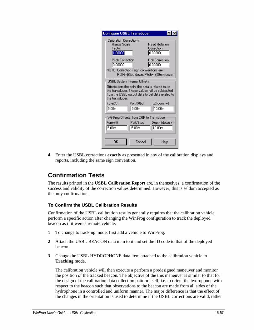
WinFrog User’s Guide – USBL Calibration 16-57
4 Enter the USBL corrections exactly as presented in any of the calibration displays and
reports, including the same sign convention.
Confirmation Tests The results printed in the USBL Calibration Report are, in themselves, a confirmation of the
success and validity of the correction values determined. However, this is seldom accepted as
the only confirmation.
To Confirm the USBL Calibration Results
Confirmation of the USBL calibration results generally requires that the calibration vehicle
perform a specific action after changing the WinFrog configuration to track the deployed
beacon as if it were a remote vehicle.
1 To change to tracking mode, first add a vehicle to WinFrog.
2 Attach the USBL BEACON data item to it and set the ID code to that of the deployed
beacon.
3 Change the USBL HYDROPHONE data item attached to the calibration vehicle to
Tracking mode.
The calibration vehicle will then execute a perform a predesigned maneuver and monitor
the position of the tracked beacon. The objective of the this maneuver is similar to that for
the design of the calibration data collection pattern itself, i.e. to orient the hydrophone with
respect to the beacon such that observations to the beacon are made from all sides of the
hydrophone in a controlled and uniform manner. The major difference is that the effect of
the changes in the orientation is used to determine if the USBL corrections are valid, rather
16-58 WinFrog User’s Guide – USBL Calibration
than to actually determine the corrections themselves. Typical maneuvers are the spin test,
where the vehicle maintains station near the beacon while rotating its heading 360°, and
simply steaming a line towards, over and away form the beacon.
If the results and application of the USBL corrections are correct, the beacon position will
remain static within a specified tolerance.
If the corrections are incorrect, the beacon’s position will appear to shift as the calibration
vehicle performs its maneuver. This shift will be correlated to the orientation of the
calibration vehicle with respect to the beacon.
Summary of the USBL Calibration Process 1 Ensure that all devices involved are operating properly and are correctly configured. These
include the USBL, GPS, gyro and attitude sensor.
2 Ensure that all devices and their associated data items are added to WinFrog and the
calibration vehicle, respectively. Confirm the configurations.
3 Ensure a valid Working Xponder file is opened.
4 Design the appropriate directory structure and file naming standard to ensure the data will be
saved in manner that is easy to understand and manage.
5 Determine the data collection pattern to use.
6 Deploy a Beacon in the calibration area, taking a fix with the surface navigation to
determine the estimated deployment location. Alternatively, if the beacon is deployed with
an ROV (standard for deep water calibrations) take several fixes using the uncalibrated
USBL system to determine an estimate for the deployment location.
7 Determine the depth of the beacon as precisely as possible.
8 Edit the Working Xponder file and ensure that a USBL Fixed beacon is present for the
deployed beacon. Enter the beacon name, estimated deployment coordinates, the best
determination of the depth (as is possible), and the beacon’s code.
9 Setup the calibration data collection in WinFrog and following the pattern, collect the data,
saving regularly to disk during the process.
10 Upon completion of the data collection. Copy the calibration file and set the copy’s
attributes to Read Only.
11 Process the data:
Beacon position determination.
- Review the data (position and range LOPs) and remove obvious bad data
based upon trends. not residuals.
- Setup and solve for the beacon position.
- Review the same data again, this time refining the editing using examination
of both the LOPs and their residuals.
- Resolve the beacon position.
- Repeat until satisfied with the results.
USBL Corrections determination
- Review the data (bearing and depth LOPs) and remove obvious bad data.
WinFrog User’s Guide – USBL Calibration 16-59
- Setup and solve for the USBL corrections.
- Review the data and refine the editing. Include the USBL report in the
examination and analysis of the results to assist the editing.
- Resolve the USBL corrections.
- Repeat until satisfied with the results.
Save the final calibration file.
Save the report to an enhanced metafile for subsequent inclusion in a
document/report.
12 Apply the results, entering the corrections in the appropriate USBL HYDROPHONE
transducer configuration, being careful to enter the data exactly as produced in the
calibration.
13 Perform a confirmation as required.
14 Perform any necessary file management and cleanup of intermediate files.
16-60 WinFrog User’s Guide – USBL Calibration
This page intentionally left blank.