CHAPTER 16Standard Deviation of a

Discrete Random Variable

First center (expected value)Now - spread

Standard Deviation of a Discrete Random Variable

Measures how “spread out” the random variable is

Summarizing data and probability

DataHistogrammeasure of the

center: sample mean x

measure of spread:sample standard deviation s

Random variableProbability

Histogrammeasure of the

center: population mean

measure of spread: population standard deviation

Example

x 0 100p(x) 1/2 1/2

E(x) = 0(1/2) + 100(1/2) = 50

y 49 51p(y) 1/2 1/2

E(y) = 49(1/2) + 51(1/2) = 50

s =

(X X)

n - 1 =

1805.703

34 = 53.10892

i2

i=1

n

VarianceVariance

The deviations of the outcomes from the mean of the probability distribution xi - µ

2 (sigma squared) is the variance of the probability distribution

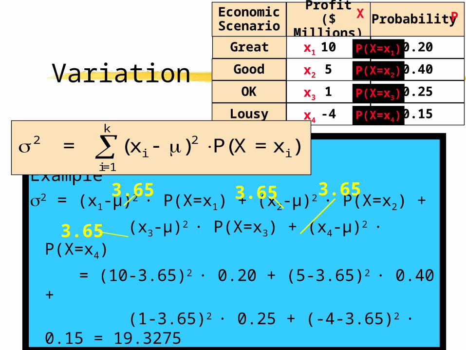
Variation

X - Xi

s =

(X X)

n - 1 =

1805.703

34 = 53.10892

i2

i=1

n

VarianceVariance

Variation

2 2

1

= ( ) ( = )=

x P X xi ii

k

Probability

Great 0.20

Good 0.40

OK 0.25

EconomicScenario

Profit($ Millions)

5

1

-4Lousy 0.15

10

P(X=x4)

X

x1

x2

x3

x4

P

P(X=x1)

P(X=x2)

P(X=x3)

P. 207, Handout 4.1, P. 4

Example2 = (x1-µ)2 · P(X=x1) + (x2-µ)2 · P(X=x2) +

(x3-µ)2 · P(X=x3) + (x4-µ)2 · P(X=x4)

= (10-3.65)2 · 0.20 + (5-3.65)2 · 0.40 + (1-3.65)2 · 0.25 + (-4-3.65)2 · 0.15 =

19.3275

Variation

3.65 3.65

3.65

3.65

2 2

1

= ( ) ( = )=

x P X xi ii

k

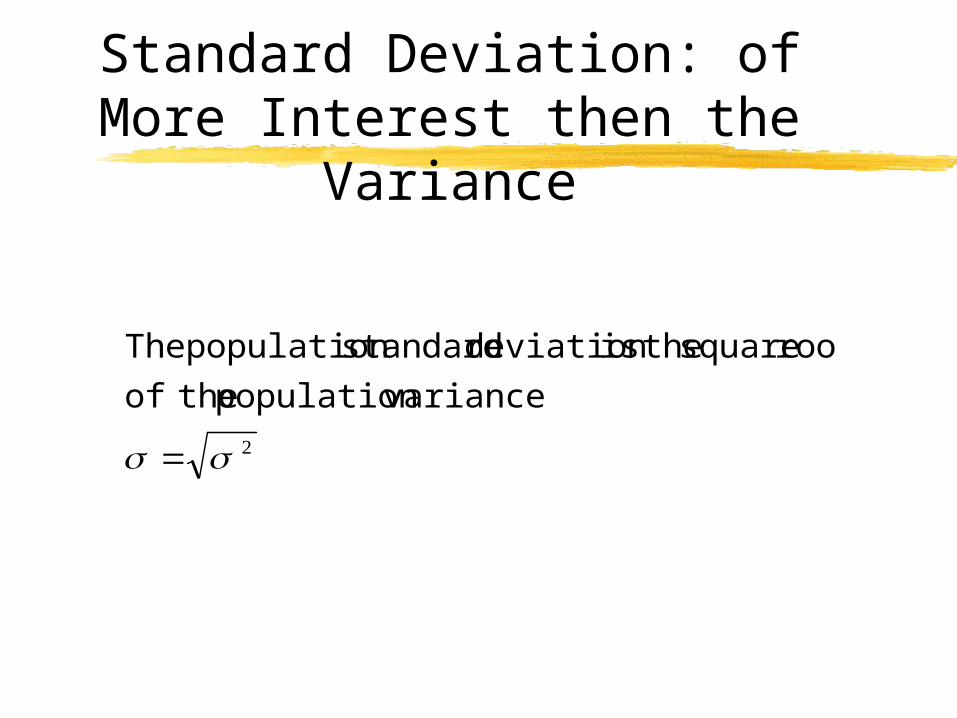
Standard Deviation: of More Interest then the Variance

variancepopulation theof

root square theisdeviation standard population The

Standard Deviation (s) =

Positive Square Root of the Variance

Standard DeviationStandard Deviation

s = s2

or SD, is the standard deviation of the probability distribution

Standard Deviation

(or SD) = 19.3275 4.40 ($ mil.)

2 = 19.3275

2 (or SD) =

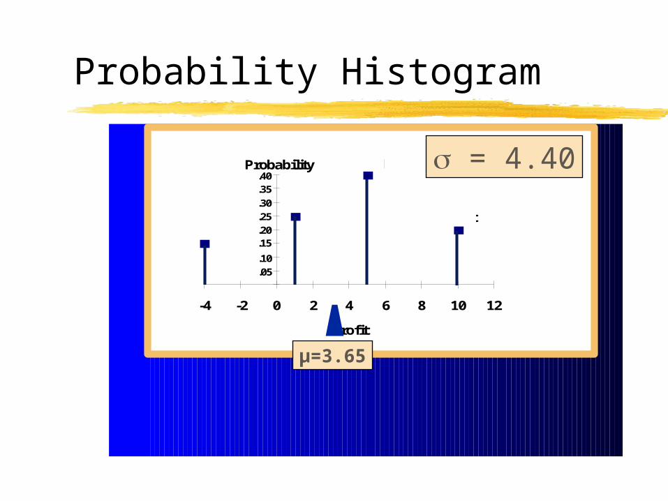
Probability Histogram

-4 -2 0 2 4 6 8 10 12

Profit

Probability

Lousy

OK

Good

Great

.05

.10

.15

.40

.20

.25

.30

.35

µ=3.65

= 4.40

Finance and Investment Interpretation

X = return on an investment (stock, portfolio, etc.)

E(x) = expected return on this investment

is a measure of the risk of the investment

Example

866.75.

.75.

25.2 25. 25. 25.2

)5.13()5.12()5.11()5.10(

: variance theCompute8

1

8

3

8

3

8

1)(

3210

81

83

83

81

812

832

832

8122

xp

x

2 2

1

= ( ) ( = )=

x P X xi ii

k

Example (cont.)Specify the interval ()(1.5 - 1(.866), 1.5 + 1(.866))

(1.5 - .866, 1.5 + .866)

(.634, 2.366)P(.634 x 2.366) = p(1)+p(2)=3/8 + 3/8 = 3/4

68-95-99.7 Rule for Random Variables

For random variables x whose probability histograms are approximately mound-shaped:

P x P x P( x

Rules for E(X), Var(X) and SD(X)adding a constant a

If X is a rv and a is a constant:

E(X+a) = E(X)+a

Example: a = -1

E(X+a)=E(X-1)=E(X)-1

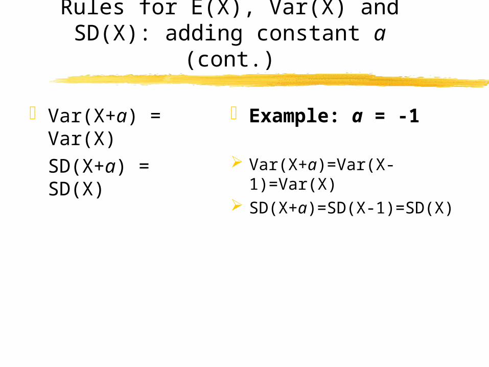
Rules for E(X), Var(X) and SD(X): adding constant a (cont.)

Var(X+a) = Var(X)SD(X+a) = SD(X)

Example: a = -1

Var(X+a)=Var(X-1)=Var(X)

SD(X+a)=SD(X-1)=SD(X)

Probability

Great 0.20

Good 0.40

OK 0.25

EconomicScenario

Profit($ Millions)

5

1

-4Lousy 0.15

10

P(X=x4)

X

x1

x2

x3

x4

P

P(X=x1)

P(X=x2)

P(X=x3)

Probability

Great 0.20

Good 0.40

OK 0.25

EconomicScenario

Profit($ Millions)

5+2

1+2

-4+2Lousy 0.15

10+2

P(X=x4)

X+2

x1+2

x2+2

x3+2

x4+2

P

P(X=x1)

P(X=x2)

P(X=x3)

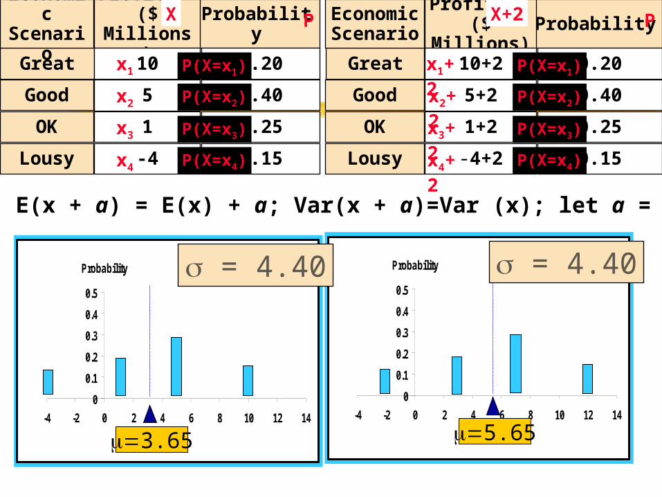
E(x + a) = E(x) + a; Var(x + a)=Var (x); let a = 2

Probability

0

0.1

0.2

0.3

0.4

0.5

-4 -2 0 2 4 6 8 10 12 14

Profit5.65

= 4.40Probability

0

0.1

0.2

0.3

0.4

0.5

-4 -2 0 2 4 6 8 10 12 14

Profit3.65

= 4.40

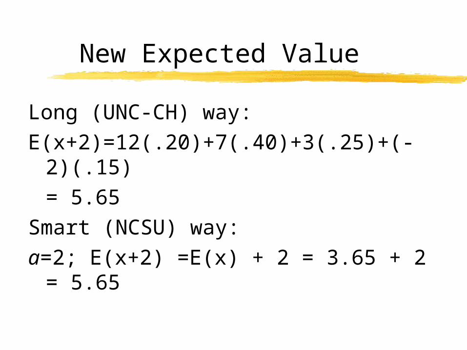
New Expected Value

Long (UNC-CH) way:E(x+2)=12(.20)+7(.40)+3(.25)+(-2)

(.15)= 5.65

Smart (NCSU) way:a=2; E(x+2) =E(x) + 2 = 3.65 + 2 =

5.65

New Variance and SDLong (UNC-CH) way: (compute from

“scratch”)Var(X+2)=(12-5.65)2(0.20)+…

+(-2+5.65)2(0.15) = 19.3275SD(X+2) = √19.3275 = 4.40

Smart (NCSU) way:Var(X+2) = Var(X) = 19.3275SD(X+2) = SD(X) = 4.40

Rules for E(X), Var(X) and SD(X): multiplying by constant b

E(bX)=b E(X)

Var(b X) = b2Var(X)

SD(bX)= |b|SD(X)

Example: b =-1 E(bX)=E(-X)=-E(X)

Var(bX)=Var(-1X)==(-1)2Var(X)=Var(X)

SD(bX)=SD(-1X)==|-1|SD(X)=SD(X)

Expected Value and SD of Linear Transformation a + bx

Let X=number of repairs a new computer needs each year. Suppose E(X)= 0.20 and SD(X)=0.55

The service contract for the computer offers unlimited repairs for $100 per year plus a $25 service charge for each repair.

What are the mean and standard deviation of the yearly cost of the service contract?

Cost = $100 + $25XE(cost) = E($100+$25X)=$100+$25E(X)=$100+$25*0.20== $100+$5=$105SD(cost)=SD($100+

$25X)=SD($25X)=$25*SD(X)=$25*0.55==$13.75

Addition and Subtraction Rules for Random Variables

E(X+Y) = E(X) + E(Y); E(X-Y) = E(X) - E(Y)

When X and Y are independent random variables:

Var(X+Y)=Var(X)+Var(Y) SD(X+Y)=

SD’s do not add:SD(X+Y)≠ SD(X)+SD(Y)

Var(X−Y)=Var(X)+Var(Y) SD(X −Y)=

SD’s do not subtract:SD(X−Y)≠ SD(X)−SD(Y)SD(X−Y)≠ SD(X)+SD(Y)

( ) ( )Var X Var Y

( ) ( )Var X Var Y

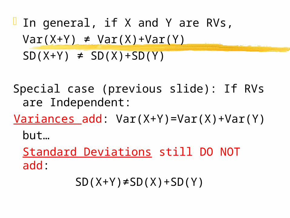
In general, if X and Y are RVs,Var(X+Y) ≠ Var(X)+Var(Y)SD(X+Y) ≠ SD(X)+SD(Y)

Special case (previous slide): If RVs are Independent:

Variances add: Var(X+Y)=Var(X)+Var(Y)but…Standard Deviations still DO NOT add:

SD(X+Y)≠SD(X)+SD(Y)

a2

c2

b2

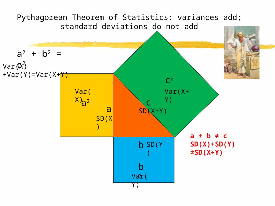
Pythagorean Theorem of Statistics: variances add; standard deviations do not add

a

b

c

a2 + b2 = c2

Var(X)

Var(Y)

Var(X+Y)

SD(X)

SD(Y)

SD(X+Y)

Var(X)+Var(Y)=Var(X+Y)

a + b ≠ cSD(X)+SD(Y) ≠SD(X+Y)

9

25

16

Pythagorean Theorem of Statistics: variances add; standard deviations do not add

3

4

5

32 + 42 = 52

Var(X)

Var(Y)

Var(X+Y)

SD(X)

SD(Y)

SD(X+Y)

Var(X)+Var(Y)=Var(X+Y)

3 + 4 ≠ 5SD(X)+SD(Y) ≠SD(X+Y)

Motivation forVar(X-Y)=Var(X)+Var(Y)

Let X=amount automatic dispensing machine puts into your 16 oz drink (say at McD’s)

A thirsty, broke friend shows up.Let Y=amount you pour into friend’s 8 oz

cup Let Z = amount left in your cup; Z = ?Z = X-YVar(Z) = Var(X-Y) =

Var(X) + Var(Y)

Has 2 components

For random variables, X+X≠2X Let X be the annual payout on a life insurance

policy. From mortality tables E(X)=$200 and SD(X)=$3,867. If the payout amounts are doubled, what are the new expected value and standard deviation?Double payout is 2X.

E(2X)=2E(X)=2*$200=$400SD(2X)=2SD(X)=2*$3,867=$7,734

Suppose insurance policies are sold to 2 people. The annual payouts are X1 and X2. Assume the 2 people behave independently. What are the expected value and standard deviation of the total payout?E(X1 + X2)=E(X1) + E(X2) = $200 + $200 =

$400

1 2 1 2 1 2

2 2

SD(X + X )= ( ) ( ) ( )

(3867) (3867) 14,953,689 14,953,689

29,907,378

Var X X Var X Var X

$5,468.76

The risk to the insurance co. when doubling the payout (2X) is not the same as the risk when selling policies to 2 people.