CHAPTER 16

Sediment budgets as an organizing framework in fluvial geomorphology

Leslie M. Reid1 and Thomas Dunne2

1USDA Forest Service Pacific Southwest Research Station, Arcata, CA, USA 2University of California, Santa Barbara, CA, USA

16.1 Introduction

Fluvial geomorphology concerns the transport of weathered rock debris and its accumulation and organization into land­forms that evolve continuously. Whereas theoretical fluvial geomorphology focuses on the mechanics of fluvial processes and the principles governing the evolution of landforms, applied fluvial geomorphology is devoted to understanding and designing strategies for coexisting with changing fluvial systems. Whenever a fluvial feature changes form, there is a local imbalance in the movement of sediment to and from the site. An understanding of how a river system collects, transports and deposits sediment is therefore central to addressing both applied and theoretical questions regarding how changes in catchment conditions affect channels, how long the effects will last and what the sequence of responses will be. Sediment budgets are tools for building that understanding. Sediment budgets define the most fundamental aspect of

landform evolution: mass conservation as it is achieved by mor­phogenetic processes acting within the boundary conditions imposed by natural or anthropogenic controls. Information about whether the sediment budget of a particular fluvial land­form or a fluvial system is in a steady state — or the degree of imbalance if it is not — is as basic a descriptor as the mean annual flood, mean annual runoff or other commonly used characterizations of fluvial systems. Quantifying sediment sup­plies and transport rates is typically more difficult to accomplish than measurement of hydroclimatic quantities, but technical advances during the past few decades have improved the capac­ity for defining the sediment budgets of fluvial systems. Even rudimentary sediment budgets can prevent oversights and guide the selection of the analytical tools needed for more detailed analyses. Eventually, the degree of detail and sophistication of sediment budgeting is constrained by time and by the avail­ability of data sources and tools, many of which are described in detail in other chapters of this book. This chapter discusses the nature of sediment budgets, provides examples of how they

have been used and describes an approach for designing and constructing useful budgets.

The sediment budget defined A sediment budget describes the input, transport, storage and export of sediment in a geomorphic system. For example, Fig. 16.1 encapsulates the operation of the sediment budget of a small forested mountain catchment. This budget was based ini­tially on qualitative field observations and mapping of sediment sources and storage elements and the conceptual diagram was then used to guide quantitative estimates of the various transfer rates and storage times of the sediment. Sediment budgets can be designed to quantify the magnitude

of a process or response rate, its location and its timing or to explore the influences contributing to a morphological change. They can be used to compare the likely outcomes of different land-management options or climatic changes or to evaluate the significance and implications of climatic, tectonic or land-use changes that have already occurred. Sediment budgets provide a framework for organizing both qualitative information about process interactions and quantitative information about process rates. Budgets can take many forms, describe many scales and incorporate diverse levels of precision. The most commonly used sediment budgets take the form of qualitative flowcharts that describe relationships between sediment sources and trans­port processes. Long-term monitoring projects often are used to provide more precise measurements of particular budget components. Whether qualitative or quantitative, all sediment budgets are

conceptually underlain by the continuity equation for sediment transfer:

sediment input to a landscape element = sediment output

+ change in sediment storage (16.1)

where all terms are expressed as quantities per unit time. The basic equation can be refined in many ways. Changes in grain

Tools in Fluvial Geomorphology, Second Edition. Edited by G. Mathias Kondolf and Hervé Piégay. © 2016 John Wiley & Sons, Ltd. Published 2016 by John Wiley & Sons, Ltd.

357

358 Chapter 16

BedrockSoil

Soil

Mixing, weathering

Creep, weathering

Creep, weathering

Saprolite Weathering

BedrockMixing, weathering Saprolite Weathering

Hollow

Foot slope debris slide

Debris flow

Sediment in

tributary channels

Debris torrent,

high stream

discharge

Debris fan

Debris fan

erosion

Sediment in main valley

Bank erosion

‘Active’ sediment in main channel

Bedload transport

Bedload discharge

Dissolved load

transport

Dissolved load

discharge

Suspended load

transport

Suspended load

discharge

Bed material attrition

Ridge

Side slope

Figure 16.1 Conceptual model of the sediment budget of a small mountainous watershed in the Oregon Coast Range. Rectangles represent storage elements, octagons indicate transfer processes and circles represent outputs. Solid lines indicate the transfer of sediment and dotted lines represent the migration of solutes. Dietrich and Dunne, 1978. Reproduced with permission of Schweizerbart.

size can be accounted for by constructing the equation for different size classes, for example, and specific processes can be isolated. Given the various forms that sediment budgets may take and

the variety of problems to which they can be applied (Table 16.1), it is clearly not useful to think of sediment budgeting as a single tool to be applied using a uniform protocol. Instead, sediment budgeting represents a general approach to geomorphic problem solving and the methods most useful for each budget depend on the intended application of that budget.

History and applications Geomorphologists have long used the concept that imbalances between sediment supply and transport capacity cause aggra­dation and degradation, and results of sediment production and transport measurements were being used to understand landscapes by the late 1800s. Hill (1896), for example, integrated the results of landslide surveys in New Zealand to demonstrate that landslides could influence landscape evolution. Gilbert (1917) used a sediment budget to evaluate the impacts of hydraulic mining in California on downstream navigation, and although later work in the same river system added detail (James 1997; Singer et al. 2013), Gilbert’s basic insight remains useful. Sediment budgeting as a concept for interpreting sparse data

soon proved useful for analysing the landscape-scale effects of land use. Both Haggett (1961) in southeastern Brazil and Trim­ble (1977) in the Southern Appalachian Mountains found large disparities between landscape-averaged estimates of soil erosion

following European colonization and subsequent amounts of fluvial sediment transport in neighbouring lowlands. Both authors interpreted the disparities to indicate that large volumes of sediment must be stored on footslopes and valley floors and would continue to contribute fluvial sediment long after hillslopes restabilize. These studies emphasized the connec­tions between sediment fluxes through landscape elements and highlighted the importance of changes in sediment storage. Although these sediment budgets were rudimentary by modern standards, they revealed the significance of long-term, inter­mittent transfer and storage of sediment throughout landscapes and stimulated decades of research. By the mid-1900s, methods had been developed to quantify

components of sediment regimes and long-term monitoring records and aerial photographs were becoming available. The idea of systematically quantifying the balance between sediment inputs, transport rates and storage changes began to spread. At first, sediment budgets simply involved systematic accounting of process measurements (for a review, see Reid and Dunne 1996). More recently, field monitoring studies were coupled with modelling to interpret, extend and generalize results. New methods of dating now allow long-term deposition rates to be evaluated for large sediment sinks and analyses of cosmogenic isotope concentrations in sediment are used to infer average erosion rates over large catchments and regions. As methodological and conceptual difficulties were sur­

mounted, the organizing power of the sediment budget concept became more evident and the approach is now widely applied to quantify landform evolution under both natural and modified

Sediment budgets as an organizing framework in fluvial geomorphology 359

Table 16.1 Examples of sediment budgets used to address issues in fluvial geomorphology.

Problem and reference Why Regime Precision Time Method PDF DESY LNS AELS MFAESH

Spatial focus: Catchment response Prioritize rehabilitation by erosion potential (Gellis et al. 2001) .D. .E.. ..S … S .FA … Proportion of sediment yield from landslides (Hovius et al. 1997) .D. .E.. .N. A … .FA … Sediment contribution to lake from cyclone (Page et al. 1994) .D. DESY .N. .E.. .FA.S. Effectiveness of soil conservation strategies (Phillips 1986) ..F DESY .N. ..L. .F. Downstream influence of upper-basin sediment (Phillips 1991) PD. DESY .N. ..L. .F. Relation of hillslope erosion to sediment yield (Reneau and Dietrich 1991) P.. .E.Y .N. A. F..SH Spatial focus: Channel system response Plan restoration using erosion distribution (Abernethy and Rutherfurd 1998) .DF DE.. L.S S .F.E.. Extent of channel recovery from old mining debris (James 1997) .DF DES. ..S ..L. MFA..H Effect of mining on downstream channels (Knighton 1991) P.F DESY .N. ..L. .FA Long-channel trends in sediment character (Le Pera and Sorriso-Valvo 2000) .D. D .N. S .F. Effect of land use on downstream channel form (Liébault and Piégay 2001) .D. .ES. .N. ..L. .FAES. Extent of channel recovery from a major flood (Madej and Ozaki 1996) P.. DESY .N. .E.. MFA Downstream distribution of mining debris (Marron 1992) P.. DES. .N. ..L. .FA.S. Effects of land use on downstream conditions (Trimble 1983) P.. DESY .N. ..L. .F.E.. Develop strategy for catchment rehabilitation (Trimble 1993) ..F DESY ..S ..L. .F.E.. Spatial focus: Response of a particular reach Cause of change in channel form (Brooks and Brierley 1997) P.. .ES. L.. ..L. .F..S. Effect of gravel mining on channel form (Collins and Dunne 1989) P.. .ES. .N. ..L. .FAE.H Design appropriate gravel harvest rate (Davis et al. 2000) .D. DES ..S S .F.E.H Sediment exchanges between channel and floodplain (Dunne et al. 1998) .D. DESY .N. A MFAE.. Describe original river sediment regime (Kesel et al. 1992) P.. .ESY .N. A ..H Particle transport mode variation through a reach (McLean et al. 1999) .D. D.SY .N. A M.. Effect of channelization on a wetland (Nakamura et al. 1997) P.. D.S. .N. ..L. MFA Effect of dam on downstream sediment load (Phillips et al. 2004) .D. DESY .N. ..L. .FAE.H Manage river to improve fish habitat (Pitlick and Van Steeter 1998) ..F DES. .N. ..L. MF.E.. Extent of sand deposition during floods (Ten Brinke et al. 1998) .D. D.S. .N. .E.. .FA Extent of deposition of suspended sediment load (Walling et al. 1998) .D. ..S. .N. S MF..S. Design dam release regime for bed material (Wilcock et al. 1996) ..F .ES. .N. A E.. Downstream effect of sediment release (Wohl and Cenderelli 2000) .D. DESY .N. .E.. MF. Effect of dams on Yangtze delta (Yang et al. 2005) .DF .ESY .NS S ..A.. Spatial focus: Specific land use, landform, etc. Controls on gully form and evolution (Harvey 1992) PDF DESY .N. A MFA Sediment input during road construction (Megahan et al. 1986) .D. .E.Y .N. ..L. M.. Effect of land use on lake sedimentation (Page and Trustrum 1997) P.. Y .N. A.L. .S. Effect of small dams on national sediment budget (Renwick et al. 2005) .D. ..SY .N. A E.H

Why: Purpose Precision Method P Explains past development L Qualitative M Monitoring carried out for the study D Describes present system N Quantitative F Field measurements or observations F Forecasts future conditions S Semiquantitative (e.g. rankings) A Aerial photograph interpretation Component of sediment regime Time considered E Modelling or published equations D Involves spatial distribution A Generalized or long-term average S Analysis of sediment deposits E Evaluates erosion E Effect of a specific event H Historical records or archived data S Evaluates sediment storage L Selected to evaluate land use Y Evaluates sediment yield S Referenced to specific period

conditions (Table 16.1). Sediment budgets now play a key role in basic and applied geomorphological studies over a wide range of scales and levels of complexity. For example, Flemings and Jordan (1989) used a model of mountain building, isostasy and crustal flexure to analyse the partitioning of sediment between an evolving orogen, the adjacent sedimentary basin and export downstream, and Church and Slaymaker (1989) illustrated the importance of lagged and indirect responses in erosion and

sedimentation during and after glaciation. Questions about the response of rivers to perturbations such as land use (Trimble 1974), dam construction and gravel mining (Kondolf and Swanson 1993) and sea-level rise (Allison et al. 1998) have also been explored by systematically accounting for input and output of sediment. Other studies have examined the exchange of sediment between channels and their floodplains (Marron 1992; Dunne et al. 1998). More recently, budgets have been used

360 Chapter 16

to predict effects of climate change (Lane et al. 2007) and to investigate the processes of carbon cycling (Cole et al. 2007). Because sediment affects many ecosystem and watershed

processes, sediment budgets can also be used to explore bio­geochemical issues. Graf (1994) and Malmon et al. (2002), for example, studied the migration of radionuclides through channels and floodplains of Los Alamos Canyon, New Mexico, noting in particular the disparate trajectories of coarse sediment that contains little contaminant and the more reactive fine sediment. Walling et al. (2003) evaluated the role of floodplain sedimentation on contaminant flux along several rivers in northern England and Singer et al. (2013) quantified the role of sediment exchanges in distributing mercury within the Central Valley of California. The fate of carbon in large river systems is another emerging target of sediment budgeting (Aufdenkampe et al. 2011) Sediment budgeting has contributed to the management of

sediment-related problems. Studies have described the effects of logging on sediment regimes through long-term monitoring (Swanson et al. 1982) and have quantified the effects of specific activities such as road construction (Megahan et al. 1986) and road use (Reid and Dunne 1984), providing information useful for targeting sediment control efforts. Sediment budgeting has been used to design strategies for catchment-scale sediment control (Phillips 1986; Trimble 1993; Gellis et al. 2001) and riparian restoration (Abernethy and Rutherfurd 1998) and to plan reservoir releases to maintain habitat for particular species (Wilcock et al. 1996; Pitlick and Van Steeter 1998). Sediment budgets for river channels have guided the establishment of appropriate gravel extraction rates (Collins and Dunne 1989; Davis et al. 2000). Dams exert a growing influence on sediment transport

regimes and downstream channel responses that impact valued resources or infrastructure. Sediment budgeting provides a tool for understanding the causes and long-term outcomes of such impacts by accounting for magnitudes and spatial distributions of sediment supplies and also changes in sediment transport, deposition and erosion (Phillips et al. 2004; Yang et al. 2005; Vericat and Batalla 2006). Impoundments remove sediment from rivers and the resulting unsatisfied transport capacity of the emerging flow often causes extensive bed degradation downstream (Williams and Wolman 1984). The extent of the degradation, however, depends on how rapidly the catchment downstream augments the supply of bed material load. In some cases, the reduction of transport capacity due to decreases in flood peaks and the supply of sediment from the undammed catchment allow the channel bed to aggrade within a short distance of the dam, beginning with fans or bar accumulations at tributary mouths. Sediment budgets are increasingly used to aid regulatory over­

sight of land-use activities. Budgets have been used to develop ‘total maximum daily load’ allocations and sediment control plans required by the US Clean Water Act for non-point-source sediment in impaired catchments. Sediment budgeting can also

aid the assessment of environmental impacts from planned projects. Downstream cumulative impacts, in particular, often result from changes in erosion, transport or deposition of sediment.

16.2 Understanding and assessing components of the sediment system

A sediment system can be examined from many points of view and each of these could be represented by a sediment budget. Which point of view is most useful depends on the intended application. To understand the variety of approaches possible and the analytical challenges they involve, the components of a catchment’s sediment production and transport system must first be understood. A wealth of literature is available about specific aspects of the sediment system and other chapters in this book discuss sediment transport and channel change. Here we summarize concepts that are particularly relevant to sedi­ment budgeting and describe assessment methods applicable to components of the sediment system. Samples of relevant references describing applications of the concepts are included in Tables 16.2 and 16.3.

Hillslope processes and sediment delivery to streams Sediment in a catchment originates from bedrock, atmospheric deposition and biological activity. Bedrock becomes sediment through physical and chemical weathering, during which some of the original material is removed by dissolution. The ‘soil pro­duction rate’ (Heimsath et al. 1997) or ‘regolith production rate’ (Small et al. 1999) is the rate per unit area at which soil material is converted from bedrock. As weathering progresses, a particle may remain in place as

saprolite or be dislodged (‘eroded’) and transported downslope as colluvium. Erosion rates are generally described as a net loss of sediment per unit area or a rate of surface lowering, whereas transport rates represent the discharge of sediment per unit width of hillslope or through a channel cross-section. Net erosion occurs only where transport into an area is less than transport out. Ordinarily, a sequence of disparate hillslope processes

(Table 16.2) moves sediment particles intermittently downs­lope to a channel. The rate of sediment production to stream channels has been defined as the rate of colluvial sediment transport across a line corresponding to the stream bank (Reid and Dunne 1996). The words ‘production’ and ‘delivery’ can refer to transfer between any landscape elements, so the context for the usage must be considered carefully to avoid confusion or double-accounting. In an accounting of primary sediment input, any particle can

be delivered to the stream system only once. For example, soil creep moves sediment to the base of a slope, where bank erosion carves away the encroaching sediment. In this case, sediment

Sediment budgets as an organizing framework in fluvial geomorphology 361

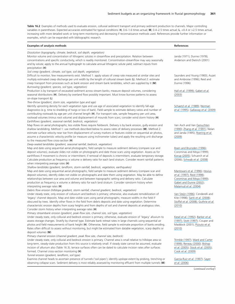
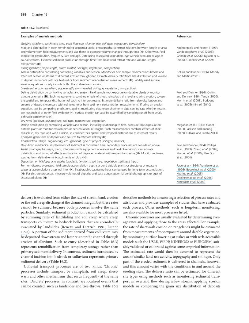
Table 16.2 Examples of methods used to evaluate erosion, colluvial sediment transport and primary sediment production to channels. Major controlling variables in parentheses. Expected accuracies estimated for typical conditions: H, 0.6–1.6 times actual; M, 0.4–2.5 times actual; L, <0.4 or >2.5 times actual, increasing with more detailed work or long-term monitoring and decreasing if reconnaissance methods used. References provide further information or examples, which can be expanded with bibliographic research.

Examples of analysis methods References

Dissolution (topography, climate, bedrock, soil depth, vegetation) Monitor volume and concentration of lithogenic solutes in streamflow and precipitation. Relation between Janda (1971); Dunne (1978); concentrations and specific conductivity, which is readily monitored. Concentration-streamflow may vary seasonally Anderson and Dietrich (2001) and by solute; apply to the annual hydrograph to calculate annual lithogenic solute yield; subtract inputs from precipitation (H) Soil creep (gradient, climate, soil type, soil depth, vegetation) Difficult to monitor; few measurements exist. Method 1: apply values of creep rate measured at similar sites and Saunders and Young (1983); Auzet multiply estimated creep discharge per unit width by the length of colluvial stream bank (L). Method 2: estimate and Ambroise (1996); Reid and creep transport from processes such as bank erosion and stream bank landslides, which are supplied by it (M) Dunne (1996) Burrowing (gradient, species, soil type, vegetation) Production is by transport of excavated sediment across stream banks; measure deposit volumes, considering Hall et al. (1999); Gabet et al. seasonal distributions (H). Delivery by overland flow possibly important. Must know burrow patterns to assess (2003) on-slope transport (L) Tree-throw (gradient, storm size, vegetation type and age) Identify uprooting density for each vegetation type and use age of associated vegetation to identify fall-age Schaetzl et al. (1989); Norman diagnostics (e.g. time to shedding of twigs or loss of bark). Field sample to estimate delivery ratios and number of et al. (1995); Gallaway et al. (2009) contributing rootwads by age per unit channel length (H). For transport rate, sample frequency per unit area, rootwad volumes (minus root volume) and displacement of mounds from scars; consider wind storm history (H) Earthflows (gradient, seasonal rainfall, bedrock, vegetation) Map flows on aerial photographs; less visible flows require fieldwork. Delivery is by bank erosion, gully erosion and Van Asch and Van Genuchten shallow landsliding. Method 1: use methods described below to assess rates of delivery processes (M). Method 2: (1990); Zhang et al. (1991); Nolan estimate surface velocity near toe from displacement of survey markers or features visible on sequential air photos, and Janda (1995); Roering et al. assume a characteristic velocity profile (or measure using inclinometer tubes) and apply the resulting unit discharge (2009) to the measured flow cross-section (H) Deep-seated landslides (gradient, seasonal rainfall, bedrock, vegetation) Map and date using sequential aerial photographs; field sample to measure sediment delivery (compare scar and Ibsen and Brunsden (1996); deposit volumes), evaluate slides not visible on photographs and date those scars using vegetation. Assess as for Corominas and Moya (1999); earthflows if movement is chronic or intermittent; if removal of deposits is intermittent, evaluate temporary storage. Korup (2005); Schuerch et al. Calculate production as frequency × volume × delivery ratio for each land stratum. Consider recent rainfall patterns (2006); Schwab et al. (2008) when interpreting average rates (H) Shallow landslides (gradient, landform, storm rainfall, bedrock, vegetation, earthquakes) Map and date using sequential aerial photographs; field sample to measure sediment delivery (compare scar and Mantovani et al. (1996); Hovius deposit volumes), identify slides not visible on photographs and date them using vegetation. May be able to define et al. (1997); Reid (1998); relationships between scar area and volume and between topographic setting and delivery ratio. Calculate Corominas and Moya (1999); production as frequency × volume × delivery ratio for each land stratum. Consider rainstorm history when Gabet and Dunne (2002); interpreting average rates (H) Malamud et al. (2004) Debris flow erosion (hillslope gradient, storm rainfall, channel gradient, bedrock, vegetation) Under steady state, only erosion of colluvium and bedrock is primary; otherwise, also evaluate remobilization of Van Steijn (1996); Cenderelli and ‘legacy’ channel deposits. Map and date visible scars using aerial photographs; measure widths in the field if Kite (1998); Santi et al. (2008); obscured by trees. Identify other flows in the field from debris deposits and date using vegetation. Determine Stoffel et al. (2008); Guthrie et al. characteristic erosion depths from scarp heights and from depths of soil and channel deposits at analogous sites. (2010) Consider storm history when interpreting average rates (H) Primary streambank erosion (gradient, peak-flow size, channel size, soil type, vegetation) Under steady state, only colluvial and bedrock erosion is primary; otherwise, evaluate erosion of ‘legacy’ alluvium to Kesel et al. (1992); Barker et al. assess storage changes. Stratify by channel type. Estimate bank retreat rates in large channels using sequential air (1997); Stott (1997); Couper and photos and field measurements of bank height (H). Otherwise, field sample to estimate proportion of banks eroding. Maddock (2001); Pizzuto et al. Rates often difficult to assess without monitoring, but might be estimated from datable vegetation, scarp depths or (2010) deposit volumes (M) Primary channel erosion (channel gradient, peak flow size, channel size, bedrock) Under steady state, only colluvial and bedrock erosion is primary. Channel area is small relative to hillslope area so Trimble (1997); Ward and Carter long-term, steady-state production from this source is relatively small. If steady state cannot be assumed, evaluate (1999); Reneau (2000); Bishop incision of alluvium also (Table 16.3); terrace surfaces often can be dated to calculate incision rates after surfaces et al. (2005); Stock et al. (2005); formed. Channel cross-section monitoring (H) Cook et al. (2009) Tunnel erosion (gradient, landform, soil type) Examine channel heads to ascertain presence of tunnels (‘soil pipes’); identify upslope extent by probing, trenching or García-Ruiz et al. (1997); Sayer observing collapse scars. Sediment delivery is most reliably assessed by monitoring effluent from multiple tunnels (M) et al. (2006)

(continued overleaf )

362 Chapter 16

Table 16.2 (continued)

Examples of analysis methods References

Gullying (gradient, catchment area, peak flow size, channel size, soil type, vegetation, compaction) Map and date gullies in open terrain using sequential aerial photographs; construct relations between length or area Nachtergaele and Poesen (1999); and volume from field measurements and use these to estimate volume changes through time (H). Otherwise, field Vandekerckhove et al. (2003); sample for distribution, frequency, size and age. Date using associated vegetation, eye-witness accounts or age of Ghimire et al. (2006); Nyssen et al. causal features. Estimate sediment production through time from headward retreat rate and volume–length (2006); Giménez et al. (2009) relationships (H) Rilling (gradient, slope length, storm rainfall, soil type, vegetation, compaction) Assess distribution considering controlling variables and season. Monitor or field sample rill dimensions before and Collins and Dunne (1986); Moody after wet season or storms of different sizes or through year. Estimate delivery ratio from size distribution and volume and Martin (2001) of deposits (compare with soil texture) or from sediment concentration measurements (H). Widely used surface erosion equations usually include both rill and sheetwash erosion Sheetwash erosion (gradient, slope length, storm rainfall, soil type, vegetation, compaction) Define distribution by controlling variables and season. Field sample root exposure on datable plants or monitor Reid and Dunne (1984); Collins using erosion pins (H). Such measurements combine effects of sheet, rainsplash, dry ravel and wind erosion, so use and Dunne (1986); Yanda (2000); the spatial and temporal distribution of each to interpret results. Estimate delivery ratio from size distribution and Merritt et al. (2003); Bodoque volume of deposits (compare with soil texture) or from sediment concentration measurements. If using an erosion et al. (2005); Kinnell (2010) equation, test by comparing predictions against monitoring data (even short-term data can indicate whether results are reasonable) or other field evidence (H). Surface erosion can also be quantified by sampling runoff from small, definable catchments (H) Dry ravel (gradient, soil moisture, soil type, temperature, vegetation) Define distribution by controlling variables and season, including relationship to fires. Measure root exposure on Megahan et al. (1983); Gabet datable plants or monitor erosion pins or accumulation in troughs. Such measurements combine effects of sheet, (2003); Jackson and Roering rainsplash, dry ravel and wind erosion, so consider their spatial and temporal distributions to interpret results. (2009); DiBiase and Lamb (2013) Compare grain sizes of deposits and sources to estimate delivery (H) Construction, tillage, engineering, etc. (gradient, type of project, soil type, bedrock) Only direct mechanical displacement of sediment is considered here; secondary processes are considered above. Reid and Dunne (1984); Phillips Aerial photographs, maps, plans, interviews with equipment operators and field observations can indicate et al. (1999); Zhang et al. (2004); distribution and timing of effects and location of displaced material with respect to streams (H). Monitor sediment Marden et al. (2006); Van Oost washed from definable mini-catchments or plots (H) et al. (2006) Deposition on hillslopes and swales (gradient, landform, soil type, vegetation, sediment input) For non-discrete processes, field sample accumulation depths around datable plants or structures or measure Page et al. (1994); Vandaele et al. seasonal accumulations atop leaf litter (H). Stratigraphic dating methods can be used for long-term accumulations (1996); Beuselinck et al. (2000); (H). For discrete processes, measure volumes of deposits and date using sequential aerial photographs or ages of Nearing et al. (2005); associated plants (H) Descheemaeker et al. (2006);

Notebaert et al. (2009)

delivery is evaluated from either the rate of stream bank erosion or the soil creep discharge at the channel margin, but these rates cannot be summed because both processes involve the same particles. Similarly, sediment production cannot be calculated by summing rates of landsliding and soil creep where creep transports colluvium to bedrock hollows that are episodically evacuated by landslides (Reneau and Dietrich 1991; Dunne 1998). A portion of the sediment derived from colluvium may be deposited downstream and later re-enter the channel through erosion of alluvium. Such re-entry (described in Table 16.3) represents remobilization from temporary storage rather than primary sediment delivery. In contrast, sediment introduced by channel incision into bedrock or colluvium represents primary sediment delivery (Table 16.2). Colluvial transport processes are of two kinds. ‘Chronic’

processes include transport by rainsplash, soil creep, sheet-wash and other mechanisms that recur frequently at the same sites. ‘Discrete’ processes, in contrast, are localized events that can be counted, such as landslides and tree-throws. Table 16.2

describes methods for measuring a selection of process rates and attributes and provides examples of studies that have evaluated each process. Other methods, such as long-term monitoring, are also available for most processes listed. Chronic processes are usually evaluated by determining aver­

age rates and applying those to the areas affected. For example, the rate of sheetwash erosion on rangelands might be estimated from measurements of root exposure around datable vegetation, by monitoring surface lowering at stakes or with web-accessible models such the USLE, WEPP, KINEROS2 or EUROSEM, suit­ably validated or calibrated against some empirical information. The estimated rate would then be assumed to represent the area of similar land-use activity, topography and soil type. Only part of the eroded sediment is delivered to channels, however, and this amount varies with the conditions in and around the eroding sites. The delivery ratio can be estimated for different site types using methods such as monitoring sediment trans­port in overland flow during a few storms, applying erosion models or comparing the grain size distribution of deposits

Sediment budgets as an organizing framework in fluvial geomorphology 363

Table 16.3 Examples of methods used to evaluate sediment transport and storage in channels, erosion of alluvial sediment and sediment yield. Major controlling variables listed in parentheses. Expected accuracies estimated for typical conditions: H, 0.6–1.6 times actual; M, 0.4–2.5 times actual; L, <0.4 or >2.5 times actual. Accuracy increases with more detailed work or long-term monitoring and decreases if reconnaissance methods are used. References selected to provide further information or examples.

Examples of analysis methods References

Bedload (channel gradient and form, flow distribution, grain size, sediment input, bedrock) Where coarse load is trapped in a lake or low-gradient reach, estimate transport by measuring temporal changes Reid and Dunne (1996); McLean and in depositional landforms using topographic surveys or aerial photographs (H). Bedload sampling data are Church (1999); Davis et al. (2000); available for a few stations, but records are usually sparse and short. Otherwise, use carefully selected bedload Brasington et al. (2003); Pelpola and transport equations, appropriate for the conditions being assessed (M) Hickin (2004); Wilcock et al. (2009) Suspended load (channel gradient and form, flow distribution, grain size, sediment input, bedrock) Measure suspended sediment concentrations over a range of flows to define a sediment rating curve and apply Reid and Dunne (1984); Asselman the resulting curve to annual hydrographs (M to H). Sediment transport equations for suspendable bed-material (2000); Moatar et al. (2006); Gao load are useful if input-dependent washload is not large (M) (2008); Wang et al. (2009) Sediment attrition (transport rate, grain size, rock type) Tumbling-mill experiments can indicate grain-size changes per unit travel distance (H). If different lithologies are Kuenen (1956); Collins and Dunne present in bed material, use changes in relative abundance to estimate relative breakdown rates (M) (1989); Lewin and Brewer (2002); Le

Pera and Sorriso-Valvo (2000) Bed aggradation (channel gradient and form, flow distribution, grain size, sediment load) Land surveys or surveys for bridge planning can be repeated; local residents can describe recent changes; and Brooks and Brierley (1997); Wathen engulfed artefacts, woody debris or plants can indicate the extent and timing of aggradation, as can changes in and Hoey (1998); Lisle and Hilton overbank flood severity. Long-term flow gauging data can document changes in bed elevation. Recently (1999); Sloan et al. (2001); Faustini aggraded bed material often is finer grained and can be probed to determine the depth to a coarser gravel layer. and Jones (2003); Lancaster and Establish timing from personal accounts, vegetation ages and comparison of sequential aerial photographs. Casebeer (2007) Estimate bar aggradation rates by multiplying the areas of bars deposited by average bar heights (H to M) Floodplain aggradation (channel gradient and form, flow history, grain size, sediment load, vegetation) Measure deposit depths around datable plants or structures or date deposits using methods described in other Ten Brinke et al. (1998); Gomez et al. chapters (H). Data from sediment traps or stakes can indicate relation between deposition and flood size, as can (1999); Rumsby (2000); Lecce and post-flood observations of deposition; data from large floods are needed to estimate long-term rates (H). Many Pavlowsky (2001); Knox (2006); Aalto methods for assessing bed aggradation can be applied to banks and floodplains. Several-decade-long cores can et al. (2008); Hoffmann et al. (2009); be dated with 137Cs concentration profiles, profiles of 210Pb attached to clay particles can provide longer records Provansal et al. (2010) and 14C dating produces records dating back thousands of years Channel erosion of alluvial sediments (channel gradient and form, flow distribution, grain size, sediment load, bedrock) Compare channel geometry to that of unaffected channels (H). Land surveys or cross-sections surveyed for James (1997); Gonzalez (2001); bridge planning can be resurveyed if available. Calculate river-bed elevation trends at gauging stations from Liébault and Piégay (2001); Miller et al. low-flow stage records and flow–depth measurements. Residents can describe recent changes and undercut (2001); Kesel (2003) vegetation or exposed bridge piers may provide data. Timing is usually established from personal accounts or comparison of sequential aerial photographs. Evaluate erosion rates from shifting of large channels by multiplying the areas of bank eroded by the average bank height. (H to M) Sediment yield (catchment size, flow distribution, sediment input, bedrock, vegetation, topography) Where catchments drain into lakes or ponds, yield can be estimated from rates of lake sedimentation if the trap Wilby et al. (1997); Lloyd et al. (1998); efficiency is known and the bathymetry has been monitored or can be reconstructed (H). Measurements or Verstraeten and Poesen (2002); calculations of sediment transport at the mouth of a catchment provide an estimate of yield (H to M). Nearby Tamene et al. (2006). catchments with similar characteristics are expected to have similar sediment yields (M)

with that of the eroding material. Sediment production rates are then calculated by multiplying hillslope sediment yields by sediment delivery ratios for each site type and applying these values to the distribution of site types present. The parameter values of predictive models, however, are known only very approximately, despite thousands of plot-years of observations. Most applications of such models result only in discrimina­tion of areas which produce large amounts of sediment and those which provide little. Nevertheless, such discrimination is often sufficient for highlighting which processes or landscape components dominate the sediment supply.

Rates of discrete processes, such as landslides, usually are evaluated by applying the measured spatial and temporal fre­quency of events to the area susceptible. Shallow landslide scars, for example, ordinarily are counted on sequential aerial photographs to determine the number of slides per unit area per unit time. Fieldwork is usually necessary to define a relationship between scar area and scar volume and to determine the propor­tion of landslide debris characteristically delivered to streams, and is also useful for estimating the frequency of landslides too small to detect on photographs. Because shallow landslides are generally triggered by infrequent, large storms, the dependence

364 Chapter 16

of areal landslide density on the magnitude of triggering events may need to be defined to determine whether the sampling period is long enough to estimate valid average rates. For many applications, only the relative rates between different land uses or landforms need be known and results from a single extensive storm often can provide this information. Analysis of other process rates generally follows similar pat­

terns (Table 16.2). The success of each rate analysis depends on (i) having a well-defined objective that identifies the informa­tion required, (ii) using a sampling design that permits valid characterization of the process and (iii) recognizing the area and time period over which the estimate applies. Wherever possible, rates should be estimated using multiple methods and should be checked for consistency; this is particularly important if rates are to be modelled in areas or under conditions for which the model has not been adequately tested.

Sediment transport in channels Changes in hillslope sediment transport arouse concern when sediment reaches a channel. Incoming sediment can modify a channel’s bed, morphology and sediment transport rates and may change the dominant transport mode. Streams transport sediment in three ways. The largest grains are rolled or jostled along the bed as ‘bedload’, while the smallest particles are continuously suspended in the flow (‘washload’). Intermediate grains are entrained repeatedly by eddies and move predomi­nantly as suspended load. These intermediate sizes return to the bed when flow slows and are referred to as ‘bed material sus­pended load’. Most sediment in the streambed represents size fractions moved as bedload (especially in gravel-bed channels) or bed material suspended load (in sand-bed channels). The transport mode for a particular grain varies with flow and with channel characteristics. Travel times for different components of the sediment load

vary widely. Washload can exit a 1500 km2 catchment during the same storm that eroded the sediment from a headwater hillslope, while bedload particles may require many decades to move the same distance. Typical long-term average annual travel distances for particles that are stored intermittently in channel beds are 100s of metres per year for gravel in small streams, 100–1000s of metres per year for gravel in large braided rivers, and 100–1000s of metres per year for sandy bedload (see studies described by Bunte and MacDonald 1999). Matisoff et al. (2002) demonstrated that concentrations of the isotopes 7Be, 137Cs and 210Pb in suspended sediment can be used to measure the speeds and distances of fine sediment transport in single flood seasons. The most accurate estimates of sediment transport rates in

channels are provided by well-designed networks of monitoring stations with records long enough to produce representative results. However, most sediment budgets must be constructed too rapidly for such monitoring to be useful unless the data already exist and can be generalized statistically. In those cases, rates can be estimated using empirical or calibrated transport

equations. Transported amounts can sometimes be obtained by measuring the volume of sediment deposited in natural or artificial sediment traps (such as alluvial fans or reservoirs) over a known period (Table 16.3). In the absence of direct measurements, theoretical trans­

port equations can provide useful estimates of non-washload components if the equations were calibrated over the range of conditions needed for the application. Reid and Dunne (1996) published comparisons between predicted and observed results and identified equations that appear to be reliable for various bed materials and channel sizes. Results are usually more accu­rate for sand-bedded than for gravel-bedded channels, but even the most reliable equations generally are accurate only to within a factor of two. Because washload is influenced more by sedi­ment availability than by flow properties, transport equations are not useful if this component is important to the problem at hand. Instead, short-term monitoring results can be used to produce sediment rating curves, which can then be combined with calculated or measured hydrographs to estimate total sus­pended sediment loads, but they can be misleading if high flows are not sampled. As with any monitoring-based method, errors are introduced if the monitoring period is unrepresentative or if estimates are made by extrapolation beyond the conditions measured. However, if applied carefully, the method is the best available for predictions of washload and probably of all suspended load. During transport, sediment grains are subject to fracture,

abrasion, weathering and dissolution, contributing to widely observed downstream decreases in grain size and shifts in particle composition. Downstream fining is also influenced by size-dependent transport and additions of sediment along the channel, so attrition rates are not directly calculable from down­stream size trends. Breakdown rates have also been estimated by measuring changes in clast size distribution as a function of ‘travel distance’ in rock tumblers that have been modified to provide realistic rates of particle interaction.

Channel and floodplain sediment storage Periods of significant sediment transport in channels are inter­spersed with much longer periods when most of the sediment is temporarily stored in the channel bed, bars and floodplains. Durations of temporary storage vary by depositional feature and by location in a catchment. Small amounts of even washload-size sediment can be trapped within the bed or bank material during transport or can infiltrate as flows recede and fine sediment carried over banks can settle quickly onto floodplains. Storage on floodplains is favoured in rivers with high concentrations of particularly fine-grained sediment. Sediment deposited on floodplains generally remains in place until eroded by chan­nel migration, so its residence time is greater where channel migration is slow. Clay, silt and fine sand are also deposited on stream banks.

Residence times can be very long if banks are well vegetated and sediment is remobilized only by bank erosion, but slumping

Sediment budgets as an organizing framework in fluvial geomorphology 365

and rilling as flows recede can reintroduce some of the newly deposited sediment. Silt and sand can accumulate on stream beds if sediment loads are particularly high or transport capacity is perennially or seasonally low. Where aggradation is triggered by an altered balance between input and transport capacity, pools commonly fill first (e.g. Lisle and Hilton 1999; Wohl and Cenderelli 2000). Gravel is usually deposited within the channel and incor­

porated into the floodplain as the channel migrates. However, unless the channel is aggrading, most coarse sediment resides in bars until the next bed-mobilizing flow moves the clasts further downstream (Hassan et al. 1991). Large increases in coarse sediment inputs to a channel network can produce temporary waveforms of gravel that can be either mobile or stationary (Jacobson and Gran 1999; Lisle et al. 2001). No landscape is unchanging, but many change slowly enough

that ‘steady-state’ rates of sediment production and deposition can be assumed over useful time-scales. Over the long term, the evolution of landforms alters rates (e.g. erosion rates may decrease as progressive erosion reduces hillslope gradients), whereas over a shorter period, weather patterns would need consideration (e.g. 10-year-old flood deposits may provide a temporary sediment source). On average, however, if no areas of chronic aggradation or incision exist downstream, sediment contributed to a stream system under steady-state conditions roughly balances the sediment exported from the catchment. In catchments with rapidly evolving landforms or changing

conditions, this simplified view must be expanded to account for changes in sediment storage (Trimble 1977). Major changes in sediment input, transport and storage can occur because of land use, hydrological regime change or the legacy of deglaciation and volcanism. Long periods may be required for re-equilibration of the system and different portions may respond out of phase with one another (e.g. Womack and Schumm 1977; Trimble 1983; Madej and Ozaki 1996). Under these conditions, both input to and output from channel storage need to be evaluated. Evalua­tion methods for erosion from storage are similar to those for erosion of hillslope materials (Table 16.3); results produce esti­mates of alluvial sediment input due to incision or changes in channel form. Rates of aggradation on streambeds, banks and floodplains can be assessed using stratigraphic and dating meth­ods described in previous chapters.

The catchment: integrating the sediment system Different parts of a catchment participate in the sediment regime in different ways. Low-order channels are often the major conduits for sediment input both because they are most closely connected with hillslopes and because they account for most of the drainage density. Downstream, channels are often inset into their own deposits. These terraces and floodplains can prevent hillslope sediment from reaching the channel directly and channels at these locations may simply rework sediment initially contributed from hillslopes upstream. Opportunities for deposition and long-term storage generally

increase downstream as alluvial valleys widen and gradients decrease. The ‘sediment yield’ is the rate of sediment output from

a catchment. Because sediment yields vary with catchment size, comparisons between catchments are usually based on yields per unit catchment area. Sediment yields per unit area frequently decrease as catchment size increases, both because average hillslope gradients decrease with increasing drainage area and because long-term aggradation is more likely down­stream. Also, short-term spatial variations in precipitation and other disturbances, together with the general inverse relation­ship between area and disturbance intensity, create localized areas of intense erosion that can far exceed the average for the entire catchment. Transport in the channel network integrates supplies from progressively larger areas of lower erosion rate in the sampling period. These effects have been conceptualized as creating a ‘sediment

delivery ratio’ for a catchment, which is defined as the propor­tion of sediment eroded from hillslopes that is exported from the catchment. If there is a permanent sediment delivery ratio of less than 1.0, the catchment is in a state of long-term geo­morphological evolution in which the high, steep uplands are being lowered relative to the lowland, which is either eroding at a slower rate or is accumulating sediment. In many catchments, however, a low sediment delivery ratio is an artefact either of the time-scale since recent disturbances or of sampling limitations. If, for example, small rainstorms during the measurement period tend to move sediment from steep areas and redeposit it on gen­tler slopes or in fans along a stream, a future wet period or major storm may compensate for the storage by scouring the sediment out of the catchment by water or debris flow. A wave of land­scape disturbance, such as described by Haggett (1961), Trim­ble (1977) and many others, may also cause the lower gradient portions of the landscape to act as filters for pulses of sediment released from steeper and more disturbed areas at rates that can­not be accommodated by the catchment-scale transport system. In still other cases, a reported sediment delivery ratio seems to be a compensating artefact to correct for the fact that erosion equations such as the USLE sometimes predict unrealistically high values of sediment supply that are inconsistent with mea­sured stream sediment transport rates or other evidence. When one is using predictive equations, it is wise to be able to iden­tify which of these interpretations of the sediment delivery ratio is appropriate. For example, if a sediment delivery ratio is used to decrease computed sediment yields in mountainous terrain, the user should be able to explain where the sediment is coming to rest. Early work within uniform physiographic regions of pre­

dominantly low relief (e.g. Maner 1958; Roehl 1962) showed sediment delivery ratios that decreased with increasing drainage area. The data defining these relationships were indirect esti­mates from the beginning. Total sediment supplies from the catchments were estimated from hillslope erosion equations and the sediment fluxes at each drainage area were measured

366 Chapter 16

by reservoir surveys corrected for trap efficiency. Although the original relationships have not been widely tested, they have been used elsewhere to estimate catchment sediment yield from evaluations of hillslope erosion. This is probably not an accurate prediction for many basins and thus requires some on-site confirmation. De Vente et al. (2007) evaluated a variety of factors that can influence downstream trends in sediment delivery ratio. Logistical and sampling difficulties have precluded much

comparison of catchment sediment yields to define their repro­ducibility and transferability. However, yields are generally expected to be similar for similar-sized catchments within an area of relatively uniform physiography, geology, climate, land use and vegetation cover, unless large, discrete sediment sources are present. For example, Dunne and Ongweny (1976) used average values for the forested, cultivated and grazed parts of a drainage basin, developed from a few gauged catchments, to identify major sources of sediment threatening the useful life of a reservoir. The results suggested that the original sediment yield estimate for the reservoir site was incorrect because of suspended sediment sampling limitations. In this case, new sampling surveys confirmed the calculations. Such an approach of transferring measurements from sampled to unmeasured

sites requires careful consideration of differences between catchments. The timing of sediment transport varies through a catchment.

Many headwater streams cannot move clasts coarser than peb­bles during frequent floods and gravel and cobbles often are trapped by woody debris. At these sites, bed material might be mobilized only when debris jams fail or during particularly large floods or debris flows. Further downstream, where bed material is finer, bed material may be mobile during ordinary bank-full events. Still further downstream, breakdown of clasts and sequestering of the larger particles lead to fining of the bed material load, until the largest rivers often transport primarily sand, silt and clay almost entirely as washload, but some fine bed material transport also occurs continuously.

16.3 Designing a sediment budget

Construction of a useful sediment budget requires the assess­ment of those parts of the sediment regime that are relevant to the particular application. No two applications have exactly the same goals or setting, so there is no single codifiable method for constructing sediment budgets. Sediment budgets vary widely in scope, approach and methods (Tables 16.1 and 16.4), and much of the skill of budget construction lies in deciding which form of

Table 16.4 Examples of options for sediment budget design. A particular sediment budget would be characterized by one or more options for each numbered attribute.

1. Purpose of budget: 5. Temporal context: 9. Landscape element: Explain landform origin Reconstruct past Hillslopes Explain change or impact Describe present Catchment Describe effect of activity Predict future Specific landform Describe effect of event Altered site Prioritize and plan remediation 6. Duration considered: Channel reach Compare systems Event-specific Channel system Predict system response Specified duration Administrative unit

Long-term average 2. Focal issue: Land-use activity 10. Material: Landform evolution Synthetic average All Land-use activity Non-dissolved Land-use effects 7. Precision: Colluvium/soil

Qualitative Suspended sediment Particular event Order-of-magnitude Bed material Particular impact Variable degree of quantification Clay/sand/gravel

Organic material 3. Target of documentation or 8. Part of sediment regime: prediction: Weathering 11. Method: Absolute amounts Hillslope transport Modelling Relative amounts Hillslope storage Compile evidence Description of interactions Erosion Inference Locations Delivery to channels Analogy/transfer Timing of response Channel storage Historical records

Channel transport Aerial photographs 4. Spatial organization: Sediment attrition Remote sensing Distributed by sites Sediment yield Stratigraphic analysis Generalized by strata Morphological features Monitoring Conceptual Lumped

Sediment budgets as an organizing framework in fluvial geomorphology 367

budget is required to address the question posed. This flexibil­ity can be a problem in applications for which the adequacy of a result is judged by whether it was obtained using standard proce­dures or where procedural manuals are expected to compensate for uneven levels of expertise. In such settings, it is critical to present a strong conceptual model of the sediment budget and to provide clear, well-documented explanations of the basis for the methods used. Table 16.4 lists various attributes of a sediment budget that can be selected for a particular purpose. Selection of appropriate options requires consideration of a suite of questions during design of the budgeting strategy (Table 16.5).

Identifying the study objectives The success of a sediment budget depends strongly on the inves­tigator’s skill in defining the focal question and identifying the information needed to answer that question. To do so, the over­all purpose for the inquiry must be understood. Are results of the sediment budget to be used for identifying the cause of an existing condition? To predict the outcome of future actions? To provide a basis for regulatory oversight? A single inquiry may have multiple interimobjectives, but careful definition of the pri­mary purpose allows the overall strategy to be optimized for that goal. If the budget is constructed as part of a broader project, the goals of the overall project also must be clearly articulated. Once the primary goal is identified, it is useful to specify how

sediment budget results will contribute to meeting that goal. This can be done by first identifying the kinds of conclusions or decisions to be made once results are available and then evaluating how different kinds of results might influence those outcomes. For example, if a project’s ultimate goal is to reduce turbidity in a trout stream, it will be necessary to decide which sediment sources to control and which options are available to control them.

Necessary and sufficient precision An evaluation of how sediment budget results are to be used also helps define the minimum level of precision required. If the result is intended to guide sediment control efforts, for example, a relative ranking of sediment sources based

on order-of-magnitude rate estimates might be sufficient. In contrast, a study to design the management of channel sedi­mentation would require more precise estimates. The necessary precision can be estimated by identifying the range in potential answers over which the decisions to be supported by the study would not be altered. If the range is wide, the precision can be low. Although many investigations would benefit from increased

precision, for many others the attainable precision is higher than that actually needed to answer the relevant questions. Pursuit of unnecessary precision drains resources from other aspects of analysis where effort might be more usefully applied.

Components to be analysed A useful sediment budget need not be complex. Most appli­cations require exploration of only a portion of the overall sediment regime. Targeting of sediment sources for control, for example, requires assessment only of sediment input rates to channels, whereas evaluation of gravel-mining influences focuses instead on changes in sediment storage in and down­stream of the affected reaches. If the intent of the budget is to determine the relative importance of a particular kind of source, it may be sufficient to evaluate the input rate from that source relative to the total sediment yield (e.g. Hovius et al. 1997), and budgets designed to address long-term landscape evolution generally describe the overall mass balance between sediment sources and sinks or net denudation rates rather than considering specific processes or sites (e.g. Matmon et al. 2003). Identification of the portion of the sediment regime requiring

study is easiest once a conceptual model has been developed for the sediment system in the area (e.g. Owens 2005). Such models have generally been in the form of flow charts (e.g. Dietrich and Dunne 1978; Reid and Dunne 1996) and tables (e.g. Kesel et al. 1992), but underlying each of these is the continuity equation for sediment transport, which simply states that, for some time interval, output equals input less any increase in storage. Constructing the relevant continuity equation for a particular application is useful because it requires the identification of rela­tionships that need to be evaluated, discloses the implications of

Table 16.5 Questions useful for guiding design of sediment budgets.

Technical questions 1. What is the overall goal of the study or project of which the sediment budget is to be a part? 2. What kinds of decisions or conclusions are expected to follow from the study’s results? 3. What information is needed to support those decisions or conclusions? 4. Are approaches other than sediment budgeting capable of providing that information? 5. What is the minimum level of precision needed to support the decisions or conclusions? 6. What is the minimum portion of the sediment regime that must be understood to support the decisions or conclusions? 7. To what area must the results apply? 8. To what period must the understanding apply? Logistical questions 9. How much time is available for the study? 10. How much funding and logistical support are available? 11. What kinds of evidence are available?

368 Chapter 16

disregarding particular components of the budget and identifies the information needed to balance the budget. Different formulations of the equation are useful for different

applications. Benda and Dunne (1997), for example, model the stochastic nature of sediment supply to reaches of channel throughout a network from landslides, debris flows and soil creep. To do so, they use a version of eqn. 16.1 modified to apply to individual reaches of third or higher order at specific times:

ΔV(k, t)Qi(k, t) + I(k, t) − Q (k, t) = (16.2)o Δt

The terms representing input (in m3 yr–1) into the channel segment k during year t are Qi(k, t), the fluvial transport (sus­pended and bed load) from upstream and I(k, t), the sum of sediment supplied to the channel segment during the year by the processes illustrated in Fig. 16.2. Q (k, t) is the corresponding oexport (m3 yr–1) from segment k during year t and the final term represents the change in the volume of sediment (V, m3) stored in segment k during year t (represented by Δt, yr). For applications involving other kinds of information, the

equation can be modified to specify the information required. For example, Dunne et al. (1998) examined interactions between the Amazon River and its floodplain (Fig. 16.2), so the equation used to organize the study separated the term describing storage into four parts, including deposition on bars within and adja­cent to the channel (Dbar), diffuse overbank deposition (Dovrbk), deposition in floodplain channels attached to the main channel (Dfpc) and deposition on the bed and banks (A 𝜌bΔz∕Δt, where cA and Δz are, respectively, the area and average elevation c change of the channel bed and banks in the reach, 𝜌b is the bulk

First-and second-order Valley side channels

1

Debris flow fan

2

5Q i(k,t)

3

4

Stream bank QO(k,t)

Figure 16.2 Conceptual model of the sediment budget of third- and higher order channel segments in the Oregon Coast Range. Sediment input processes include (1) shallow landsliding and debris flows in first- and second-order channels, (2) fluvial erosion and transport in first- and second-order channels, (3) bank erosion of debris flow fans and terraces, (4) soil creep along toeslopes of hillsides and (5) landslides from streamside hollows. Qi (k, t) and Q (k, t) represent the annual fluxes of sediment load into o

and out of the kth segment in year t. Source: Benda and Dunne, 1997. Reproduced with permission from AGU.

density of the bedmaterial and Δt is the time interval of the com­putation):

∑ Qu + Qtribi + Ebk = Qd + Dbar + Dovrbk

i

Δz+ Dfpc + Ac𝜌b + 𝜀 (16.3)Δt

where Qu, Qd and Qtrib are, respectively, the annual fluxes of sus­pended and bedload sediment at the upstream and downstream ends of each channel reach and from the i tributaries entering the reach, Ebk is bank erosion and 𝜀 is the error; each term has units of millions of tons per year. This equation, also, was formulated to apply to particular reaches, but in this case the results define the average annual balance of sediment transport of each grain size for each reach. Once the underlying equation has been defined, flowcharts are

useful for organizing specific information about processes. Pre­liminary information about major erosion and transport pro­cesses is usually available for a study area or for similar settings. This information and field inspection can be used to identify potential sediment inputs, outputs and storage changes in the area and to diagram interactions between transport processes and storage elements, with primary focus on aspects of the sed­iment regime on which the study is to concentrate (e.g. Fig. 16.3 and Fig. 9.6 in Chapter 9).

Spatial scale of analysis The most useful spatial analysis strategy for a particular study depends on the kind of area to which results are to be applied. The relevant area might be a real location (e.g. a specific catch­ment, channel reach or administrative district) or a hypothet­ical location (e.g. a ‘typical’ catchment or reach). If the budget is to explain conditions at a particular site, details of that site are often critical to the problem. The location of tributary inputs in a channel reach, for example, may strongly influence the function­ing of the sediment budget, at least in the short term. Similarly, for budgets developed to explore landform evolution, informa­tion concerning process rates must be distributed over that land-form. Geographic information systems (GIS) are useful for con­structing these spatially registered sediment budgets. However, for other applications, this level of spatial specificity is unnec­essary and results can be presented as averages for particular land types, land uses, sub-catchments or entire catchments. Bud­gets constructed for hypothetical settings, which are often used for comparing outcomes from different planning options, can be either spatially distributed or averaged. A preliminary evaluation of the spatial distribution of pro­

cesses usually simplifies budget construction by allowing the study area to be ‘stratified’ into areas that are likely to behave uniformly with respect to a particular process. Variables that control the rate or distribution of processes (Tables 16.2 and 16.3) provide a useful basis for stratification; these often include geological substrate and vegetation type for hillslope pro­cesses and channel order and geological substrate for channels.

Tributary input

Flo

odpla in channe

l Floodplain lake

Sediment budgets as an organizing framework in fluvial geomorphology 369

Suspended sediment

input Local tributary

Bar deposition

Upstream bedload

transport

Bank erosion

Overbank deposition Suspended

sediment output

Downstream bedload transport

Figure 16.3 Components of the budget of channel–floodplain sediment exchanges for ∼ 200 km long reaches of the Amazon River, Brazil. Source: Dunne et al, 1998. Reproduced with permission of Geological Society of America.

In practice, 3–10 stratification units for each process are usu­ally sufficient to facilitate analysis without over-simplifying the problem and a single stratification scheme often applies to multiple processes. Various methods have been used for stratification, ranging from visual delineations using aerial pho­tographs to automated methods using GIS-based information and satellite images (e.g. Fernández et al. 1999; Giles 1998). For most applications, process rates and distribution are most efficiently evaluated using statistically based sampling within strata; rarely are complete inventories necessary. Stratification allows both generalization of results across wider

areas and estimation of values for particular sub-areas, and can also be used to construct budgets for hypothetical conditions. In each case, results are calculated according to the distribution of strata in the area of interest.

Temporal scale of analysis Appropriate temporal scales can be selected for sediment budgets by considering the intended applications and the time-scales over which conditions change in the study area. A budget designed to examine the effects of land use on landslid­ing might evaluate landslide distribution after a single major storm on lands undergoing different uses. In contrast, a budget intended to estimate a long-term average would assess rates over a period long enough to either evaluate or average out year-to-year variations. Budgets that evaluate changes in average sediment input rel­

ative to background conditions must consider two time-scales, the first to assess long-term average natural rates, the second to provide an analogous estimate of impacted rates. Where

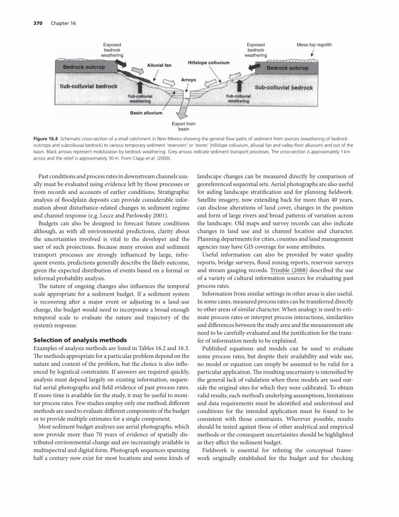
current conditions are changing rapidly, as is the case where land-use patterns are shifting, definition of a ‘long-term average’ for current conditions requires the assessment of the hypothet­ical response of the current land-use pattern to the long-term average distribution of triggering events. If landslide rates are defined as a function of storm size, for example, landslide inci­dence can be evaluated for the distribution of storms expected over a century in order to calculate the average sediment input expected if recent conditions were to be maintained for 100 years (Fig. 16.4). Comparison of current with background conditions requires

estimates of process rates active under conditions no longer present. Where nearby catchments remain in a relatively pris­tine condition, sediment budgets for pristine and disturbed conditions can be compared directly, but usually with signif­icant uncertainty due to stochastic influences, such as storm occurrence. Comparisons are most feasible for catchments of similar, small size. Consequently, processes characteristic of downstream reaches often cannot be directly compared using this strategy. More commonly, pristine examples are unavailable and

catchments or hillslopes undergoing different intensities of land use are examined instead. Analysis of trends along the gradient of land-use intensities then allows inferences about pre-disturbance conditions. A gradient of hillslope conditions usually exists even where land use is uniformly distributed between catchments, so rates of hillslope processes usually can be compared even where comparison of downstream processes is not possible.

370 Chapter 16

Exposed bedrock

weathering

Bedrock outcrop Hillslope colluviumAlluvial fan

Arroyo

Basin alluvium

Export from basin

Exposed Mesa top regolith bedrock

weathering

Bedrock outcrop

Figure 16.4 Schematic cross-section of a small catchment in New Mexico showing the general flow paths of sediment from sources (weathering of bedrock outcrops and subcolluvial bedrock) to various temporary sediment ‘reservoirs’ or ‘stores’ (hillslope colluvium, alluvial fan and valley-floor alluvium) and out of the basin. Black arrows represent mobilization by bedrock weathering. Grey arrows indicate sediment transport processes. The cross-section is approximately 1 km across and the relief is approximately 30 m. From Clapp et al. (2000).

Past conditions and process rates in downstream channels usu­ally must be evaluated using evidence left by those processes or from records and accounts of earlier conditions. Stratigraphic analysis of floodplain deposits can provide considerable infor­mation about disturbance-related changes in sediment regime and channel response (e.g. Lecce and Pavlowsky 2001). Budgets can also be designed to forecast future conditions

although, as with all environmental predictions, clarity about the uncertainties involved is vital to the developer and the user of such projections. Because many erosion and sediment transport processes are strongly influenced by large, infre­quent events, predictions generally describe the likely outcome, given the expected distribution of events based on a formal or informal probability analysis. The nature of ongoing changes also influences the temporal

scale appropriate for a sediment budget. If a sediment system is recovering after a major event or adjusting to a land-use change, the budget would need to incorporate a broad enough temporal scale to evaluate the nature and trajectory of the system’s response.

Selection of analysis methods Examples of analysis methods are listed in Tables 16.2 and 16.3. The methods appropriate for a particular problem depend on the nature and context of the problem, but the choice is also influ­enced by logistical constraints. If answers are required quickly, analysis must depend largely on existing information, sequen­tial aerial photographs and field evidence of past process rates. If more time is available for the study, it may be useful to moni­tor process rates. Few studies employ only one method; different methods are used to evaluate different components of the budget or to provide multiple estimates for a single component. Most sediment budget analyses use aerial photographs, which

now provide more than 70 years of evidence of spatially dis­tributed environmental change and are increasingly available in multispectral and digital form. Photograph sequences spanning half a century now exist for most locations and some kinds of

landscape changes can be measured directly by comparison of georeferenced sequential sets. Aerial photographs are also useful for aiding landscape stratification and for planning fieldwork. Satellite imagery, now extending back for more than 40 years, can disclose alterations of land cover, changes in the position and form of large rivers and broad patterns of variation across the landscape. Old maps and survey records can also indicate changes in land use and in channel location and character. Planning departments for cities, counties and land management agencies may have GIS coverage for some attributes. Useful information can also be provided by water quality

reports, bridge surveys, flood zoning reports, reservoir surveys and stream gauging records. Trimble (2008) described the use of a variety of cultural information sources for evaluating past process rates. Information from similar settings in other areas is also useful.

In some cases, measured process rates can be transferred directly to other areas of similar character. When analogy is used to esti­mate process rates or interpret process interactions, similarities and differences between the study area and the measurement site need to be carefully evaluated and the justification for the trans­fer of information needs to be explained. Published equations and models can be used to evaluate

some process rates, but despite their availability and wide use, no model or equation can simply be assumed to be valid for a particular application. The resulting uncertainty is intensified by the general lack of validation when these models are used out­side the original sites for which they were calibrated. To obtain valid results, each method’s underlying assumptions, limitations and data requirements must be identified and understood and conditions for the intended application must be found to be consistent with those constraints. Wherever possible, results should be tested against those of other analytical and empirical methods or the consequent uncertainties should be highlighted as they affect the sediment budget. Fieldwork is essential for refining the conceptual frame­

work originally established for the budget and for checking

Sediment budgets as an organizing framework in fluvial geomorphology 371

aerial photographic interpretations. Evaluation of most chronic sediment sources requires fieldwork and fieldwork often reveals unexpected measurement opportunities. Fieldwork also allows interviews with local observers and experts at the sites of interest; general recollections can become very specific in the presence of identifiable landmarks. Fieldwork is most usefully approached both with a prioritized list of tasks to be accom­plished and with an eye to finding opportunities to answer the focal questions more effectively. If possible, fieldwork should be scheduled for periods when important processes are likely to be active. Dry-season fieldwork, for example, is rarely useful for evaluating the distribution or even existence of overland flow. Monitoring is sometimes useful during budget construction.

Long-term average process rates can be defined through mon­itoring either if the study duration is long enough to account for temporal variations in rate (e.g. Trimble 1999) or if results define a relation between a process rate and its driving variables that allows the long-term rate to be calculated from a known distribution of driving variables (Reid and Dunne 1984; Clayton and Megahan 1986; Reid 1998). Short-term monitoring also can be useful for testing event-based modelling predictions. Comparison of modelled and monitored results for the range of sampled events indicates the level of confidence that can be placed on modelled results for unsampled events. Short-term monitoring can also reveal differences in process rates between particular site types or treatments. For any of these applica­tions, enough sites should be monitored to provide adequate confidence that results are characteristic of the relevant site type during the monitoring period. Statistical analysis of preliminary results can identify the necessary sample size.

Integrating the results Sediment budgets commonly incorporate disparate kinds of information and each information source usually represents a different temporal or spatial scale and a different granularity and data quality. The overall budget must reconcile these differences to produce an internally consistent, interpretable result. Particular care must be taken to avoid mismatching time­

scales within a budget. Sediment budget results cannot be compared or components of a single budget combined if they represent time periods that are radically different in length or environmental conditions. For example, sediment budgets commonly incorporate monitoring data, modelling results and retrospective rate estimates. If a budget is to be checked by comparing results with 2 years of sediment yield measurements, each kind of information would need to be evaluated in such a way that results apply to that 2-year period. Differences in spatial analysis scales are usually accounted for

by stratification. A single budget, for example, might include an aerial photograph inventory of road-related landslides through­out a catchment and modelled sheet erosion rates from road surfaces on two soil types. Overall rates for both sources would vary through time as the road system developed, so inputs would be calculated per unit length of road. The average annual

landslide delivery would be calculated as the total landslide delivery divided by the road-kilometre-years present during the period for which aerial photographs are available. Similarly, sheet erosion would be calculated by applying the modelled rates for each soil type to the road-kilometre-years present for that soil type during the period of aerial photographic coverage. Results could then be combined to estimate either the total input from these sources over the period of aerial photographic coverage or the combined average rate per unit length of road per year. In general, inventory data can be used directly after suitable

spatial and temporal averaging, while information characteriz­ing particular land strata or site types is applied according to the distribution of those site types. Data that are randomly sampled without regard to site type characterize the area as a whole and cannot be used to describe portions of the sample area unless the random sampling disclosed relationships between rates and controlling variables. This pattern is also true for sampling through time: a process rate evaluated as a long-term average cannot be assumed to apply to a particular interval within the analysis period.

Auditing the sediment budget An answer is not useful if it is not possible to determine whether it is likely to be true. Most sediment budgets represent a com­plex mix of calculations, mapping, measurements and qualita­tive inferences, so standard methods of error analysis are rarely applicable. Instead, results usually are tested by comparing esti­mated with measured sediment yields, assessing the reliability of each of the methods used or carrying out sensitivity analyses. The effectiveness of each approach depends on the kind of error present. The most serious errors generally result from overlooking

important processes and this can be avoided only through careful fieldwork. It is useful to begin with a complete list of major processes, identify the evidence needed to demonstrate their presence and determine whether such evidence is present. Occasionally, comparison of the summed components of the budget with a known output reveals an imbalance, but uncer­tainties in components are often too large for shortfalls to be revealed. Problems have also arisen when a difficult-to-evaluate compo­

nent was estimated as an unmeasured residual by subtracting the other components from a measured total. This approach implic­itly assumes that all components have been identified and that the cumulative error in the sum is small enough that the differ­ence between the sum and the total is meaningful (Kondolf and Matthews 1991). If such an approach is used, a sensitivity anal­ysis should be carried out to identify the potential error in the result and the presence or absence of all potential budget com­ponents should be carefully verified. Uncertainties can remain, however, even when the sediment

budget is to be defined completely by empirical methods and even in reaches of river channel where one would assume that

372 Chapter 16

it is easier than elsewhere in the landscape to characterize and measure the various components. Both the sediment fluxes in and out of a reach and the volume of storage change are usually small residuals obtained from much larger absolute values and errors in each component are squared and summed to obtain the uncertainty in the final residual. Erwin et al. (2012) demonstrated the difficulty, at least for a single flood, using unusually precise measurements of bedload transport into and out of a 4 km long reach of the gravel-bed Provo River, Utah. Even considering the uncertainties in the transport rates, their measurements indicated that influx was an order of magnitude greater than efflux, so storage must have increased. When the researchers tried to locate the resulting change in storage with a combination of ground survey and remote sensing, they were unable to demonstrate rigorously that storage had in fact increased, although its most probable value was 1.6 times that derived from the flux estimates and equivalent to only 5 mm of depth change averaged over the reach. Maps of the change in storage also revealed coherent patterns. The greatest uncertainty therefore was in the average value, rather than the existence, of accumulation within the reach for the single flood. It remains to be seen how many floods would create enough storage to be statistically recognizable with the technology available for measuring such small changes in bed elevation. Topping et al. (2000) and Grams and Schmidt (2005) described even more challenging data limitations on larger rivers over longer periods. Important errors also occur when decisions are founded

on budget results that are mistakenly assumed to be precise and accurate. In many cases, a sensitivity analysis would have revealed the uncertainty in the budget and decisions could have been tempered to reflect that uncertainty or further work done to reduce it. Large errors in individual budget components have occurred

when modelling results were relied on without field evaluation or when short-term rates were assumed to represent long-term averages. Both of these approaches are inherently unreliable and can be identified through technical review. Where such meth­ods are considered necessary, it is important that the associated uncertainty be evaluated and reported. Although no single approach to testing budget results, or other

empirical method, can ensure that the result is accurate, each is useful. Where estimated and measured sediment yields agree, the major components are not likely to be severely over- or underestimated, although compensating errors can occur. For any such test to be valid, clearly the estimates of sediment yield must be completely independent of analysis of budget com­ponents. Methods of ‘fingerprinting’ deposited or transported sediments to identify their provenance (Collins et al. 1998; Hill et al. 1998; Collins and Walling 2004) (see also Chapter 9) can be used to test portions of the overall budget. Even technically valid sediment budgets can mislead if the

question addressed by the budget is not relevant to the under­lying problem. Central to formulation of a useful question is a strong understanding of what the problem to be addressed

actually is. For problems associated with land-use activities, identified technical problems are often merely symptoms of underlying social, political or economic problems (Rossi 1998) and technical solutions that do not consider underlying causes will not be workable over the long term.

Assessing uncertainty The reliability of specific methods used in budget construction usually can be assessed from the performance of a method at other sites or from other knowledge of process rates. In some cases, reliability can be expressed as a confidence interval, whereas in others only a maximum likely error can be estimated. If multiple methods are used to estimate the same budget com­ponent, discrepancies between methods indicate the maximum potential accuracy for the suite of methods used. In some cases, formal error propagation analysis is possible for

parts of a budget. The sediment budget for the Amazon River (Fig. 16.2) (Dunne et al. 1998), for example, was constructed to allow such analysis. Equation 16 was first simplified to

∑ Qu + Qtribi − Qd =

ΔV + 𝜀 (16.4) i Δt

where Qu, Qd and Qtrib are, respectively, the annual fluxes of suspended and bedload sediment at the upstream and down­stream ends of each channel reach and from the i tributaries entering the reach and ΔV∕Δt represents the rate of change of the total sediment volume in storage in the reach. Sediment rat­ing curves and flow duration curves available for each station on the main channel and each tributary were then used to analyse error propagation for the fluvial transport terms, allowing eval­uation of the uncertainties in estimating ΔV∕Δt. The standard errors of the ΔV∕Δt terms for individual reaches differed sig­nificantly from zero for the sand fraction inmany reaches where the geomorphic and hydrological setting, and also independent estimates of the individual processes of sediment exchange, sug­gested that net erosion or deposition would occur. This was not generally the case for the larger silt–clay fraction, although subtle trends in net storage of this fraction did correlate with the same geomorphic and hydrological patterns. Also, the standard error of the storage estimate for the entire 2000 km floodplain reach (200 Mt yr–1) differed significantly from zero for both size frac­tions and it agreed approximately with the storage of 500 Mt yr–1

estimated by quantifying each term in eqn. 16.2. However, the paucity of information available for specific storage fluxes pre­vented formal estimation of uncertainties for terms describing individual exchanges between channel and floodplain. The various kinds of information used to construct a sediment

budget ordinarily incorporate very different kinds and levels of uncertainty, so a standard calculation of uncertainty usually is not possible for the overall result. Instead, the sensitivity of the result to likely levels of uncertainty in the budget components can be assessed by recalculating the result for their estimated ranges of uncertainty. For some components, the uncertainty will be represented by a 95% confidence interval; for others,

Sediment budgets as an organizing framework in fluvial geomorphology 373

it may reflect a maximum likely error or complete removal of the component from consideration. Such calculations can indicate which components of the budget require the most careful analysis. It is useful to distinguish between a result and the conclusions

to which it leads. For example, a result might be a tabulation of sediment input by process, from which it is concluded that sediment control efforts should target road-surface erosion. This distinction allows the evaluation of how much a result must change before the conclusion is affected. The range in values for the result over which the conclusion would remain unchanged defines the operationally significant tolerance interval around the result (Reid and Page 2003).

16.4 Examples

To illustrate the variety of methods and strategies available for constructing sediment budgets, it is useful to examine two contrasting examples of how particular options were selected to address specific questions (Table 16.6). The first example represents a reconnaissance-level, order-of-magnitude budget, whereas the second incorporates more detailed analysis and higher levels of precision.

Evaluating sediment production from a hurricane in Hawaii In 1992; Hurricane Iniki hit the 1325 km2 island of Kauai, in the Hawaiian Islands. Officials wanted to know whether and where the hurricane might have increased future flood hazard by reducing channel capacity through aggradation. A sediment budget study was undertaken to determine whether significant aggradation was likely, to identify endangered areas and to suggest hazard reduction measures (Reid and Smith 1992). The impacts of the hurricane were to be evaluated, so the

budget had to be event-based (Table 16.6). Results did not need to be precise; comparison of the order of magnitude of sediment

inputs to ‘normal’ values would be sufficient to determine the likelihood of a problem. Results needed to be spatially dis­tributed to identify sites at risk. The necessary spatial resolution was at the scale of the 18 major catchments because vulnerable communities and structures are concentrated at catchment mouths. Calculations within each catchment could be spatially generalized. The relevant standard of comparison for this application

ordinarily would be the volume of sediment that the rivers can remove without undergoing significant change in form. If Iniki contributed more than this volume, aggradation could result. Aggradation was not a major problem before Iniki and single rainstorms with recurrence intervals of 100 years or less have triggered landsliding and sediment loading of at least an average year’s sediment yield. It was therefore assumed that downstream aggradation would not occur if the hurricane had contributed less than an average year’s sediment load to a river. The standard of comparison then became the average annual sediment input in years without hurricanes. Sediment yields have not been measured on Kauai, but various estimates suggest that yields range between 300 and 3000 t km–2 yr–1 and the distribution of old landslide scars suggests that years with intense storms have produced considerably higher yields. Landslides were mapped by comparing 1:12,000 colour

infrared aerial photographs taken before and after the storm. Most landslides triggered by the hurricane displaced only the soil profile and their average depth was estimated from average soil depths. The hurricane was relatively dry, so excess sheet erosion could have occurred only in areas bared by the hur­ricane, which were restricted to landslide scars. Trees blown down into streams carried sediment with their roots and these were mapped from a helicopter in streams wider than 5 m. The average frequency of blown-down trees was then extrapolated to smaller drainages. The volume of sediment carried by each rootwad was estimated from field observations. Sheetwash erosion rates, depths of soil removed by landslides and rootwad

Table 16.6 Examples of strategies selected for two sediment budgeting applications (see Table 16.4 for other options).

Sediment budget Hurricane Iniki budget Clearwater road budget attribute (Reid and Smith 1992) (Reid et al. 1981)

1. Purpose of budget Prioritize, plan remediation Prioritize, plan remediation 2. Focal issue Particular event and impact Particular land-use activity and

impact 3. Form of results Relative amounts Absolute amounts 4. Spatial organization Distributed by catchments Hypothetical 5. Temporal context Describe present Describe present 6. Duration considered Event-specific Synthetic average 7. Precision Order of magnitude Precise 8. Part of regime Erosion Delivery to channels 9. Landscape element Catchment Land-use activity sites 10. Material Non-dissolved Non-dissolved 11. Method Modelling, aerial photographs, Monitoring, aerial

existing evidence photographs, existing evidence

374 Chapter 16

Table 16.7 An order-of-magnitude sediment budget for sediment contributed by Hurricane Iniki to catchments and hydrological zones on the island of Kauai, Hawaii. Expected annual sediment inputs are on the order of 1000 t km–2 yr–1.

Watershed or zone Increased sediment input from hurricane

Sheet erosion Landslides Uprooting Total

1. Wainiha ++ +++ + +++ 2. Lumahai ++ +++ + +++ 3. Waioli – – + + 4. Hanalei – – + + 5. Kalihiwai – – + + 6. Kilauea – – + + 7. Anahola – + + ++ 8. Kapaa – + + + 9. Wailua – + + ++ 10. Hanamaulu – – + + 11. Huleia – – + + 12. Waikomo – – + + 13. Lawai – – + + 14. Wahiawa – – + + 15. Hanapepe ++ ++ + ++ 16. Canyon zone – – + + 17. Waimea + ++ + ++ 18. Na Pali zone ++ ++ + ++

Symbols: –, <1 t km–2; +, 1–10 t km–2; ++, 10–100 t km–2; +++, 100–1000 t km–2. Adapted from Reid and Smith (1992).

volumes were represented by likely maximum values so that results would represent the maximum potential input. The orders of magnitude of the estimated storm inputs

were then compared with expected average annual inputs (Table 16.7). Sediment inputs from Iniki were found to be potentially significant only in the two watersheds that contained large debris flows, but even there the storm-related sediment input was of the same order as an average year’s input and so not likely to cause aggradation. On this basis, it was recommended that channel cross-sections be monitored periodically at poten­tially vulnerable locations, but that major mitigation efforts for sediment were not necessary. In all, the budget was constructed using about 10 hours of helicopter time, one day of fieldwork and one week of office work.

Prioritizing erosion control on roads in the Olympic Mountains, Washington, USA The 375 km2 Clearwater watershed, located in the Olympic Mountains of Washington State, is intensively managed for timber production by the Washington Department of Natural Resources. The Clearwater River is an important source of salmon and earlier work suggested that the presence of roads is associated with impairment of spawning habitat because fine-grained sediment eroded from roads accumulates in spawning gravels. Department staff needed to know the most important sources of road-related sediment in order to select effective erosion-control measures, so a sediment budget was constructed to evaluate the relative importance of road-related sediment sources in the area (Reid et al. 1981). Work on the budget required less than one person-year distributed over a 2-year period.

The only portion of the sediment regime that required analysis was sediment production to streams. The budget focused on fine-grained sediment, which had been identified as the major problem and sources not related to roads could be excluded. Results could be in the form of long-term average inputs and so did not need to be related to particular sites or time periods. The budget could therefore be spatially generalized. Because relative values were the major concern, only a moderate level of precision was needed. Road-related landslide, sidecast erosion, gully and debris

flow rates were evaluated for two watersheds using road con­struction records and three sequences of aerial photographs. Delivery ratios for these sources were assessed by measuring the volumes of sediment deposits at a selection of field sites and secondary erosion on landslide scars was estimated from root exposure and erosion pin measurements. Road-surface erosion was evaluated by sampling effluent from 10 culverts during 17 storms of various sizes and defining relations between sediment concentration and discharge for different intensities of road use. Similar measurements on a paved road segment allowed the isolation of roadcut and ditch erosion rates and these were also estimated from measurements at stakes and root exposures on roadcut surfaces. Only the erosion pins required a lengthy monitoring period and they turned out to be unnecessary because root exposure measurements provided analogous data representing a much longer effective sampling period. Culvert hydrographs were reconstructed for unsampled

storms using unit hydrographs. The discharge–concentration relationships then allowed estimation of the sediment yield for each storm over an 11-year period (Reid and Dunne 1984).

Sediment budgets as an organizing framework in fluvial geomorphology 375

Delivery ratios for road-surface, ditch and roadcut sediment were estimated by determining the proportion of culverts that contribute flow directly to streams in the area. Sediment pro­duction from landslides, sheetwash and roadcut erosion was then calculated as an annual rate per kilometre for an average distribution of road types in a hypothetical 20 km2 watershed, taking into account the distribution of road types and use intensities present in the area. Expected yields for any specific watershed could be calculated using the road distribution actually present. Because relations were quantified between road-surface sediment yields, storm intensities and traffic levels, average yields can be estimated for particular years and future yields can be estimated from projected use levels. The results identify the sediment sources in most need of

control: road-surface erosion and landslides each produce 10 times as much sediment as other sources (Table 16.8), while roadcut erosion is relatively unimportant, unlike conditions at some times in some other forested areas (Megahan et al. 1983, 1986). The results also show the importance of road use in generating sediment and quantify the impact of curtailing use during wet weather.

Table 16.8 Road-related production of sand and silt in a hypothetical 20 km2 watershed in the Clearwater basin. Road density is 2.5 kmkm–2, including a representative distribution of road-use intensities: 6% heavily used, 5% moderately used, 39% lightly used and 50% abandoned. Heavily used roads fall into the ‘temporary non-use’ category at night and weekends.

Source Fine sediment production (t km–2 yr–1)

Landslides 40 Debris flows∗ 6.6 Gullies 0.4 Sidecast erosion 2.8 Secondary surface erosion on slide scars 12 Rills on landslide scars 3.2 Roadcut erosion† (4.0)†

Road surface and roadcut: Heavy use 36 Temporary non-use 5.2 Moderate use 5.2 Light use 3.7 Abandoned 0.6

Total 116

∗Only valley-wall erosion by debris flows is listed here; the triggering landslide is included in the land­slide category. †Roadcut erosion is included in the values for ‘Road surface and roadcut’, but is listed separately here to allow comparison. After Reid et al. (1981).

16.5 Conclusions

Recent studies demonstrate the utility of the sediment budgeting approach for addressing a wide range of theoretical and applied problems in fluvial geomorphology (Table 16.1). The most efficiently constructed and effective budgets have been those designed to incorporate the kind and precision of information necessary and sufficient to address the questions posed. Only with a carefully defined focus can the appropriate options for budget construction be selected from the wide array available, and only with carefully defined objectives can the reliability of the resulting budget be assessed.

References

Aalto, R., Lauer, J.W. and Dietrich, W.E. 2008. Spatial and temporal dynamics of sediment accumulation and exchange along Strickland River floodplains (Papua New Guinea) over decadal-to-centennial timescales. Journal of Geophysical Research 113: F01S04.

Abernethy, B. and Rutherfurd, I.D. 1998. Where along a river’s length will vegetation most effectively stabilise stream banks? Geomorphol­ogy 23(1):55–75.

Allison, M.A., Kuehl, S.A., Martin, T.C. and Hassan, A. 1998. Impor­tance of floodplain sedimentation for river sediment budgets and ter­rigenous input to the ocean: insights from the Brahmaputra–Jamuna River. Geology 26(2): 175–178.

Anderson, S.P. and Dietrich, W.E. 2001. Chemical weathering and runoff chemistry in a steep headwater catchment. Hydrological Processes 15: 1791–1815.

Asselman, N.E.M. 2000. Fitting and interpretation of sediment rating curves. Journal of Hydrology 234(3–4): 228–248.

Aufdenkampe, A.K., Mayorga, E., Raymond, P.A., Melack, J.M., Doney, S.C., Alin, S.R., Aalto, R.E. and Yoo, K. 2011. Riverine coupling of bio­geochemical cycles between land, oceans and atmosphere. Frontiers in Ecology and the Environment 9(1): 53–60.

Auzet, A.-V. and Ambroise, B. 1996. Soil creep dynamics, soil moisture and temperature conditions on a forested slope in the granitic Vos­ges Mountains, France. Earth Surface Processes and Landforms 21(6): 531–542.

Barker, R., Dixon, L. and Hooke, J. 1997. Use of terrestrial photogram­metry for monitoring and measuring bank erosion. Earth Surface Pro­cesses and Landforms 22(13): 1217–1227.

Benda, L. and Dunne, T. 1997. Stochastic forcing of sediment storage and routing in channel networks. Water Resources Research 33(12): 2865–2880.

Beuselinck, L., Steegen, A., Govers, G., Nachtergaele, J., Takken, I. and Poesen, J. 2000. Characteristics of sediment deposits formed by intense rainfall events in small catchments in the Belgian Loam Belt. Geomorphology 32(1–2): 69–82.

Bishop, P., Hoey, T.B., Jansen, J.D. and Artza, I.L. 2005. Knickpoint recession rate and catchment area: the case of uplifted rivers in Eastern Scotland. Earth Surface Processes and Landforms 30: 767–778.

Bodoque, J.M., Díez-Herrero, A., Martín-Duque, J.F., Rubiales, J.M., Godfrey, A., Pedraza, J., Carrasco, R.M. and Sanz, M.A. 2005. Sheet erosion rates determined by using dendrogeomorphological analysis

376 Chapter 16

of exposed tree roots: two examples from Central Spain. Catena 64(1): 81–102.

Brasington, J., Langham, J. and Rumsby, B. 2003. Methodological sensi­tivity of morphometric estimates of coarse fluvial sediment transport. Geomorphology 53: 299–316.

Brooks, A.P. and Brierley, G.J. 1997. Geomorphic responses of lower Bega River to catchment disturbance, 1851–1926. Geomorphology 18(3–4): 291–304.

Bunte, K. and MacDonald L.H. 1999. Scale Considerations and the Detectability of Sedimentary Cumulative Watershed Effects, Technical Bulletin 776, Research Triangle Park, NC: National Council of the Paper Industry for Air and Stream Improvement, 327pp.

Cenderelli, D.A. and Kite, J.S. 1998. Geomorphic effects of large debris flows on channel morphology at North Fork Mountain, Eastern West Virginia. Earth Surface Processes and Landforms 23(1): 1–20.

Church, M. and Slaymaker, O. 1989. Disequilibrium of Holocene sedi­ment yield in glaciated British Columbia. Nature 337: 452–454.

Clapp, E.M., Bierman, P.R., Schick, A.P., Lekach, J., Enzel, Y. and Caffee, M. 2000. Sediment yield exceeds sediment production in arid region drainage basins. Geology 28: 995–998.

Clayton, J.L. and Megahan, W.F. 1986. Erosional and chemical denuda­tion rates in the southwestern Idaho Batholith. Earth Surface Processes and Landforms 11(4): 389–400.

Cole, J.J., Prairie, Y.T., Caraco, N.F., McDowell, W.H., Tranvik, L.J., Striegl, R.G., Duarte, C.M., Kortelainen, P., Downing, J.A., Mid­delburg, J.J. and Melack, J. 2007. Plumbing the global carbon cycle: integrating inland waters into the terrestrial carbon budget. Ecosystems 10: 171–184.

Collins, A.L. and Walling, D.E. 2004. Documenting catchment sus­pended sediment sources: problems, approaches and prospects. Progress in Physical Geography 28(2): 159–196.

Collins, B.D. and Dunne, T. 1986. Erosion of tephra from the 1980 erup­tion of Mount St. Helens. Geological Society of America Bulletin 97(7): 896–905.

Collins, B.D. and Dunne, T. 1989. Gravel transport, gravel harvest­ing and channel-bed degradation in rivers draining the southern Olympic Mountains, Washington, USA. Environmental Geology and Water Science 13(3): 213–224.

Collins, A.L., Walling, D.E. and Leeks, G.J.L. 1998. Use of composite fingerprints to determine the provenance of the contemporary sus­pended sediment load transported by rivers. Earth Surface Processes and Landforms 23(1): 31–52.

Cook, K.L., Whipple, K.X., Heimsath, A.M. and Hanks, T.C. 2009. Rapid incision of the Colorado River in Glen Canyon – insights from chan­nel profiles, local incision rates and modeling of lithologic controls. Earth Surface Processes and Landforms 34(7): 994–1010.

Corominas, J. and Moya, J. 1999. Reconstructing recent landslide activ­ity in relation to rainfall in the Llobregat River basin, Eastern Pyre­nees, Spain. Geomorphology 30(1–2): 79–93.

Couper, P.R. and Maddock, I.P. 2001. Subaerial river bank erosion processes and their interaction with other bank erosion mechanisms on the River Arrow, Warwickshire, UK. Earth Surface Processes and Landforms 26(6): 631–646.

Davis, J., Bird, J., Finlayson, B. and Scott, R. 2000. The management of gravel extraction in alluvial rivers: a case study from the Avon River, southeastern Australia. Physical Geography 21(2): 133–154.

Descheemaeker, K., Nyssen, J., Rossi, J., Poesen, J., Haile, M., Raes, D., Muys, B., Moeyersons, J. and Deckers, S. 2006. Sediment deposition

and pedogenesis in exclosures in the Tigray highlands, Ethiopia. Geo­derma 132(3–4): 291–314.

De Vente, J., Poesen, J., Arabkhedri, M. and Verstraeten, G. 2007. The sediment delivery problem revisited. Progress in Physical Geography 31(2): 155–178.

DiBiase, R.A. and Lamb, M.P. 2013. Vegetation and wildfire controls on sediment yield in bedrock landscapes. Geophysical Research Letters 40: 1093–1097.

Dietrich, W.E. and Dunne, T. 1978. Sediment budget for a small catch­ment in mountainous terrain. Zeitschrift für Geomorphologie, Supple­ment Band 29: 191–206.

Dunne, T. 1978. 1978. Rates of chemical denudation of silicate rocks in Kenya. Nature 274: 244–246.

Dunne, T. 1998. Critical data requirements for prediction of erosion and sedimentation in mountain drainage basins. Journal of the American Water Resources Association 34(4): 795–808.

Dunne, T. and Ongweny, G.S.O. 1976. A new estimate of sediment yields in the upper Tana catchment. The Kenya Geographer 2: 109–126.

Dunne, T., Mertes, L.A.K., Meade, R.H., Richey, J.E. and Forsberg, B.R. 1998. Exchanges of sediment between the flood plain and the channel of the Amazon River in Brazil. Geological Society of America Bulletin 110(4): 450–467.

Erwin, S.O., Schmidt, J.C., Wheaton, J.M. and Wilcock, P.R. 2012. Clos­ing a sediment budget for a reconfigured reach of the Provo River, Utah, United States. Water Resources Research 48(10): W10512.

Faustini, J.M. and Jones, J.A. 2003. Influence of large woody debris on channel morphology and dynamics in steep, boulder-rich moun­tain streams, western Cascades, Oregon. Geomorphology 51(1–3): 187–205.

Fernández, C.I., del Castillo, T., Hamdouni, R.E. and Montero, J.C. 1999. Verification of landslide susceptibility mapping: a case study. Earth Surface Processes and Landforms 24(6): 537–544.

Flemings, P.B. and Jordan, T.E. 1989. A synthetic stratigraphic model of foreland basin development. Journal of Geophysical Research 94(B4): 3851–3866.

Gabet, E.J. 2003. Sediment transport by dry ravel. Journal of Geophysical Research 108(B1): 2049.

Gabet, E.J. and Dunne, T. 2002. Landslides on coastal sage-scrub and grassland hillslopes in a severe El Nino winter: the effects of vegeta­tion conversion on sediment delivery. Geological Society of America Bulletin. 114: 983–990.

Gabet, E.J., Reichman, O.J. and Seabloom, E.W. 2003. The effects of bio­turbation on soil processes and sediment transport. Annual Review of Earth and Planetary Sciences 31: 249–273.

Gallaway, J.M., Martin, Y.E. and Johnson, E.A. 2009. Sediment transport due to tree root throw: integrating tree population dynamics, wild­fire and geomorphic response. Earth Surface Processes and Landforms 34(9): 1255–1269.

Gao, P. 2008. Understanding watershed suspended sediment transport. Progress in Physical Geography 32(3): 243–263.

García-Ruiz, J.M., Lasanta, T. and Alberto, F. 1997. Soil erosion by piping in irrigated fields. Geomorphology 20(3–4): 269–278.

Gellis, A.C., Cheama, A. and Lalio, S.M. 2001. Developing a geomor­phic approach for ranking watersheds for rehabilitation, Zuni Indian Reservation, New Mexico. Geomorphology 37(1–2): 105–134.

Ghimire, S.K., Higaki, D. and Bhattarai, T.P. 2006. Gully erosion in the Siwalik Hills, Nepal: estimation of sediment production from active

Sediment budgets as an organizing framework in fluvial geomorphology 377

ephemeral gullies. Earth Surface Processes and Landforms 31(2): 155–165.

Gilbert, G.K. 1917. Hydraulic-mining Débris in the Sierra Nevada, US Geological Survey Professional Paper 105, Washington, DC: US Gov­ernment Printing Office, 154pp.

Giles, P.T. 1998. Geomorphological signatures: classification of aggre­gated slope unit objects from digital elevation and remote sensing data. Earth Surface Processes and Landforms 23(7): 581–594.

Giménez, R., Marazolff, I., Campo, M.A., Seeger, M., Ries, J.B., Casalí, J. and Álvarez-Mozos, J. 2009. Accuracy of high-resolution photogram­metric measurements of gullies with contrasting morphology. Earth Surface Processes and Landforms 34(14): 1915–1926.

Gomez, B., Eden, D.N., Hicks, D.M., Trustrum, N.A., Peacock, D.H. and Wilmshurst, J. 1999. Contribution of floodplain sequestration to the sediment budget of the Waipaoa River, New Zealand. In: Marriott, S.B. and Alexander, J., eds., Floodplains: Interdisciplinary Approaches. Special Publication 163, London: Geological Society of London, pp. 69–88.

Gonzalez, M.A. 2001. Recent formation of arroyos in the Little Missouri Badlands of southwestern North Dakota. Geomorphology 38(1–2): 63–84.

Graf, W.L. 1994. Plutonium and the Rio Grande: Environmental Change and Contamination in the Nuclear Age, New York: Oxford University Press, 329pp.

Grams, P.E. and Schmidt, J.C. 2005. Equilibrium or indeterminate? Where sediment budgets fail: sediment mass balance and adjustment of channel form, Green River downstream from Flaming Gorge Dam, Utah and Colorado. Geomorphology 71(1–2): 156–181.

Guthrie, R.H., Hockin, A., Colquhoun, L., Nagy, T., Evans, S.G. and Ayles, C. 2010. An examination of controls on debris flow mobil­ity: evidence from coastal British Columbia. Geomorphology 114(4): 601–613.

Haggett, P.E. 1961. Land-use and sediment yield in an old plantation tract of the Serra do Mar, Brazil. Geographical Journal 127(1): 50–62.

Hall, K., Boelhouwers, J. and Driscoll, K. 1999. Animals as erosion agents in the alpine zone: some data and observations from Canada, Lesotho and Tibet. Arctic, Antarctic and Alpine Research 31(4): 436–446.

Harvey, A.M. 1992. Process interactions, temporal scales and the devel­opment of hillslope gully systems: Howgill Fells, northwest England. Geomorphology 5(3–5): 323–344.

Hassan, M.A., Church, M. and Schick, A.P. 1991. Distance of movement of coarse particles in gravel bed streams. Water Resources Research 27(4): 503–511.

Heimsath, A.M., Dietrich, W.E., Nishiizumi, K. and Finkel, R.C. 1997. The soil production function and landscape equilibrium. Nature 388: 358–361.

Hill, B.R., DeCarlo, E.H., Fuller, C.C. and Wong, M.F. 1998. Using sed­iment ‘fingerprints’ to assess sediment-budget errors, North Halawa Valley, Oahu, Hawaii, 1991–1992. Earth Surface Processes and Land­forms 23(6): 493–508.

Hill, H. 1896. Denudation as a factor of geologic time. Transactions and Proceedings of the New Zealand Institute 28(11th of New Series): 666–679.

Hoffmann, T., Erkens, G., Gerlach, R., Klostermann, J. and Lang, A. 2009. Trends and controls of Holocene floodplain sedimentation in the Rhine catchment. Catena 77(2): 96–106.

Hovius, N., Stark, C.P. and Allen, P.A. 1997. Sediment flux from a moun­tain belt derived by landslide mapping. Geology 25(3): 231–234.

Ibsen, M.-L. and Brunsden, D. 1996. The nature, use and problems of historical archives for the temporal occurrence of landslides, with specific reference to the south coast of Britain, Ventnor, Isle of Wight. Geomorphology 15(3–4): 241–258.

Jackson, M. and Roering, J.J. 2009. Post-fire geomorphic response in steep, forested landscapes: Oregon Coast Range, USA. Quaternary Science Reviews 28(11–12): 1131–1146.

Jacobson, R.B. and Gran, K.B. 1999. Gravel sediment routing from widespread, low-intensity landscape disturbance, Current River Basin, Missouri. Earth Surface Processes and Landforms 24(10): 897–917.

James, L.A. 1997. Channel incision on the Lower American River, Cali­fornia, from streamflow gage records. Water Resources Research 33(3): 485–490.

Janda, R.J. 1971. An evaluation of procedures used in computing chem­ical denudation rates. Geological Society of America Bulletin 82(1): 67–80.

Kesel, R.H. 2003. Human modifications to the sediment regime of the Lower Mississippi River flood plain. Geomorphology 56(3–4): 325–334.

Kesel, R.H., Yodis, E.G. and McCraw, D.J. 1992. An approximation of the sediment budget of the lower Mississippi River prior to major human modification. Earth Surface Processes and Landforms 17(7): 711–722.

Kinnell, P.I.A. 2010. Event soil loss, runoff and the Universal Soil Loss Equation family of models: a review. Journal of Hydrology 385(1–4): 384–397.

Knighton, A.D. 1991. Channel bed adjustment along mine-affected rivers of northeast Tasmania. Geomorphology 4(3–4): 205–219.

Knox, J.C. 2006. Floodplain sedimentation in the Upper Mississippi Valley: natural versus human accelerated. Geomorphology 79(3–4): 286–310.

Kondolf, G.M. and Matthews, W.V.G. 1991. Unmeasured residuals in sediment budgets: a cautionary note. Water Resources Research 27(9): 2483–2486.

Kondolf, G.M. and Swanson, M.L. 1993. Channel adjustments to reser­voir construction and gravel extraction along Stony Creek, California. Environmental Geology 21(4): 256–269.

Korup, O. 2005. Large landslides and their effect on sediment flux in South Westland, New Zealand. Earth Surface Processes and Landforms 30(3): 305–323.

Kuenen, P.H. 1956. Experimental abrasion of pebbles. 2. Rolling by cur­rent. Journal of Geology 64: 336–368.

Lancaster, S.T. and Casebeer, N.E. 2007. Sediment storage and evacu­ation in headwater valleys at the transition between debris-flow and fluvial processes. Geology 35(11): 1027–1030.

Lane, S.N., Tayefi, V., Reid, S.C., Yu, D. and Hardy, R.J. 2007. Interactions between sediment delivery, channel change, climate change and flood risk in a temperate upland environment. Earth Surface Processes and Landforms 32(3): 429–446.

Lecce, S.A. and Pavlowsky, R.T. 2001. Use of mining-contaminated sed­iment tracers to investigate the timing and rates of historical flood plain sedimentation. Geomorphology 38(1–2): 85–108.

Le Pera, E. and Sorriso-Valvo, M. 2000. Weathering, erosion and sedi­ment composition in a high-gradient river, Calabria, Italy. Earth Sur­face Processes and Landforms 25(3): 277–292.

378 Chapter 16

Lewin, J. and Brewer, P.A. 2002. Laboratory simulation of clast abrasion. Earth Surface Processes and Landforms 27(2): 145–164.

Liébault, F. and Piégay, H. 2001. Assessment of channel changes due to long-term bedload supply decrease, Roubion River, France. Geomor­phology 36(3–4): 167–186.

Lisle, T.E. and Hilton, S. 1999. Fine bed material in pools of natural gravel bed channels. Water Resources Research 35(4): 1291–1304.

Lisle, T.E., Cui, Y., Parker, G., Pizzuto, J.E. and Dodd, A.M. 2001. The dominance of dispersion in the evolution of bed material waves in gravel-bed rivers. Earth Surface Processes and Landforms 26(13): 1409–1420.

Lloyd, S.D., Bishop, P. and Reinfelds, I. 1998. Shoreline erosion: a cau­tionary note on using small farm dams to determine catchment ero­sion rates. Earth Surface Processes and Landforms 23(10): 905–912.

Madej, M.A. and Ozaki, V. 1996. Channel response to sediment wave propagation and movement, Redwood Creek, California, USA. Earth Surface Processes and Landforms 21(10): 911–927.

Malamud, B.D., Turcotte, D.L., Guzzetti, F. and Reichenbach, P. 2004. Landslide inventories and their statistical properties. Earth Surface Processes and Landforms 29(6): 687–711.

Malmon, D.V., Dunne, T. and Reneau, S.L. 2002. Predicting the fate of sediment and pollutants in river floodplains. Environmental Science and Technology 36(9): 2026–2032.

Maner, S.B. 1958. Factors influencing sediment delivery rates in the Red Hills physiographic area. EOS American Geophysical Union Transac­tions 39: 669–675.

Mantovani, F., Soeters, R. and Van Westen, C.J. 1996. Remote sensing techniques for landslide studies and hazard zonation in Europe. Geo­morphology 15(3–4): 213–225.

Marden, M., Rowan, D. and Phillips, C. 2006. Sediment sources and delivery following plantation harvesting in a weathered volcanic ter­rain, Coromandel Peninsula, North Island, New Zealand. Australian Journal of Soil Research 44(3): 219–232.

Marron, D.C. 1992. Floodplain storage of mine tailings in the Belle Fourche River system: a sediment budget approach. Earth Surface Processes and Landforms 17(7): 675–685.

Matisoff, G., Bonniwell, E.C. and Whiting, P.J. 2002. Radionuclides as indicators of sediment transport in agricultural watersheds that drain to Lake Erie. Journal of Environmental Quality 31(1): 62–72.

Matmon, A., Bierman, P.R., Larsen, J., Southworth, S., Pavich, M. and Caffee, M. 2003. Temporally and spatially uniform rates of erosion in the southern Appalachian Great Smoky Mountains. Geology 31(2): 155–158.

McLean, D.G. and Church, M. 1999. Sediment transport along lower Fraser River: 2. Estimates based on the long-term gravel budget. Water Resources Research 35(8): 2549–2559.

McLean, D.G., Church, M. and Tassone, B. 1999. Sediment transport along lower Fraser River: 1. Measurements and hydraulic computa­tions. Water Resources Research 35(8): 2533–2548.

Megahan, W.F., Seyedbagheri, K.A. and Dodson, P.C. 1983. Long-term erosion on granitic roadcuts based on exposed tree roots. Earth Sur­face Processes 8(1): 19–28.

Megahan, W.F., Seyedbagheri, K.A., Mosko, T.L. and Ketcheson, G.L. 1986. Construction phase sediment budget for forest roads on granitic slopes in Idaho. In: Hadley, R., ed., Drainage Basin Sedi­ment Delivery, IAHS Publication No. 159, Wallingford: International Association of Hydrological Sciences, pp. 31–39.

Merritt, W.S., Letcher, R.A. and Jakeman, A.J. 2003. A review of ero­sion and sediment transport models. Environmental Modelling and Software 18: 761–799.

Miller, J., Germanoski, D., Waltman, K., Tausch, R. and Chambers, J. 2001. Influence of late Holocene hillslope processes and landforms on modern channel dynamics in upland watersheds of central Nevada. Geomorphology 38(3–4): 373–391.

Moatar, F., Person, G., Meybeck, M., Coynel, A., Etcheber, H. and Crouzet, P. 2006. The influence of contrasting suspended particulate matter transport regimes on the bias and precision of flux estimates. Science of the Total Environment 370(2–3): 515–531.

Moody, J.A. and Martin, D.A. 2001. Initial hydrologic and geomorphic response following a wildfire in the Colorado Front Range. Earth Sur­face Processes and Landforms 26(10): 1049–1070.

Nachtergaele, J. and Poesen, J. 1999. Assessment of soil losses by ephemeral gully erosion using high-altitude (stereo) aerial pho­tographs. Earth Surface Processes and Landforms 24(8): 693–706.

Nakamura, F., Sudo, T., Kameyama, S. and Jitsu, M. 1997. Influences of channelization on discharge of suspended sediment and wetland veg­etation in Kushiro Marsh, northern Japan. Geomorphology 18(3–4): 279–289.

Nearing, M.A., Kimoto, A., Nichols, M.H. and Ritchie, J.C. 2005. Spatial patterns of soil erosion and deposition in two small, semiarid water­sheds. Journal of Geophysical Research 110, F04020.

Nolan, K.M. and Janda, R.J. 1995. Movement and Sediment Yield of Two Earthflows, Northwestern California, US Geological Survey Pro­fessional Paper 1454-F, Washington, DC: US Government Printing Office, 12pp.

Norman, S.A., Schaetzl, R.J. and Small, T.W. 1995. Effects of slope angle on mass movement by tree uprooting. Geomorphology 14(1): 19–27.

Notebaert, B., Verstraeten, G., Rommens, T., Vanmontfort, B., Govers, G. and Poesen, J. 2009. Establishing a Holocene sediment budget for the river Dijle. Catena 77(2): 150–163.

Nyssen, J., Poesen, J., Veyret-Picot, M., Moeyersons, J., Haile, M., Deck­ers, J., Dewit, J., Naudts, J., Teka, K. and Govers, G. 2006. Assessment of gully erosion rates through interviews and measurements: a case study from northern Ethiopia. Earth Surface Processes and Landforms 31(2): 167–185.

Owens, P.N. 2005. Conceptual models and budgets for sediment man­agement at the river basin scale. Journal of Soils and Sediments 5(4): 201–212.

Page, M.J. and Trustrum, N.A. 1997. A late Holocene lake sediment record of the erosion response to land use change in a steepland catchment, New Zealand. Zeitschrift für Geomorphologie N.F. 41(3): 369–392.

Page, M.J., Trustrum, N.A. and Dymond, J.R. 1994. Sediment budget to assess the geomorphic effect of a cyclonic storm, New Zealand. Geo­morphology 9(3): 169–188.

Pelpola, C.P. and Hicken, E.J. 2004. Long-term bed load transport rate based on aerial-photo and ground penetrating radar sur­veys of fan-delta growth, Coast Mountains, British Columbia. Geomorphology 57(3–4): 169–181.

Phillips, J.D. 1986. The utility of the sediment budget concept in sedi­ment pollution control. Professional Geographer 38(3): 246–252.

Phillips, J.D. 1991. Fluvial sediment budgets in the North Carolina Pied­mont. Geomorphology 4: 231–241.

Sediment budgets as an organizing framework in fluvial geomorphology 379

Phillips, J.D., Slattery, M.C. and Gares, P.A. 1999. Truncation and accre­tion of soil profiles on coastal plain croplands: implications for sedi­ment redistribution. Geomorphology 28(1–2): 119–140.

Phillips, J.D., Slattery, M.C. and Musselman, Z.A. 2004. Dam-to-delta sediment inputs and storage in the lower Trinity River, Texas. Geo­morphology 62(1–2): 17–34.

Pitlick, J. and Van Steeter, M.M. 1998. Geomorphology and endan­gered fish habitats of the upper Colorado River 2. Linking sediment transport to habitat maintenance. Water Resources Research 34(2): 303–316.

Pizzuto, J., O’Neal, M. and Stotts, S. 2010. On the retreat of forested, cohesive riverbanks. Geomorphology 116(3–4): 341–352.

Provansal, M., Villiet, J., Eyrolle, F., Raccasi, G., Gurriaran, R. and Antonelli, C. 2010. High-resolution evaluation of recent bank accretion rate of the managed Rhone: a case study by multi-proxy approach. Geomorphology 117(3–4): 287–297.

Reid, L.M. 1998. Calculation of average landslide frequency using cli­matic records. Water Resources Research 34(4): 869–877.

Reid, L.M. and Dunne, T. 1984. Sediment production from forest road surfaces. Water Resources Research 20(11): 1753–1761.

Reid, L.M. and Dunne, T. 1996. Rapid Evaluation of Sediment Budgets, Reiskirchen: Catena Verlag, 164pp.

Reid, L.M. and Page, M.J. 2003. Magnitude and frequency of landsliding in a large New Zealand catchment. Geomorphology 49(1–2): 71–88.

Reid, L.M. and Smith, C.W. 1992. The Effects of Hurricane Iniki on Flood Hazard on Kauai, Report to the Hawaii Department of Land and Nat­ural Resources, Honolulu, Hawaii, 26pp.

Reid, L.M., Dunne, T. and Cederholm, C.J. 1981. Application of sedi­ment budget studies to the evaluation of logging road impact. Journal of Hydrology (New Zealand) 20(1): 49–62.

Reneau, S.L. 2000. Stream incision and terrace development in Frijoles Canyon, Bandelier National Monument, New Mexico and the influ­ence of lithology and climate. Geomorphology 32(1–2): 171–193.

Reneau, S.L. and Dietrich, W.E. 1991. Erosion rates in the southern Ore­gon Coast Range: evidence for an equilibrium between hillslope ero­sion and sediment yield. Earth Surface Processes and Landforms 16(4): 307–322.

Renwick, W.H., Smith, S.V., Bartley, J.D. and Buddemeier, R.W. 2005. The role of impoundments in the sediment budget of the contermi­nous United States. Geomorphology 71(1–2): 99–111.

Roehl, J.W. 1962. Sediment Source Areas, Delivery Ratios and Influencing Morphological Factors, IAHS Publication No. 59, Wallingford: Inter­national Association of Scientific Hydrology, pp. 202–213.

Roering, J.L., Stimely, L.L., Mackey, B.H. and Schmidt, D.A. 2009. Using DInSAR, airborne LiDAR and archival air photos to quantify landsliding and sediment transport. Geophysical Research Letters 36: L19402.

Rossi, G. 1998. Erosions differ. Zeitschrift fürGeomorphologieN.F. 42(3): 297–305.

Rumsby, B. 2000. Vertical accretion rates in fluvial systems: a compari­son of volumetric and depth-based estimates. Earth Surface Processes and Landforms 25(6): 617–631.

Santi, P.M., deWolfe, V.G., Higgins, J.D., Cannon, S.H. and Gartner, J.E. 2008. Sources of debris flow material in burned areas. Geomorphology 96: 310–321.

Saunders, I. and Young, A. 1983. Rates of surface processes on slopes, slope retreat and denudation. Earth Surface Processes and Landforms 8(5): 473–501.

Sayer, A.M., Walsh, R.P.D. and Bidin, K. 2006. Pipeflow suspended sed­iment dynamics and their contribution to stream sediment budgets in small rainforest catchments, Sabah, Malaysia. Forest Ecology and Management 224(1–2): 119–130.

Schaetzl, R.J., Johnson, D.J., Burns, S.F. and Small, T.W. 1989. Tree uprooting: review of terminology, process and environmental implications. Canadian Journal of Forest Research 19(1): 1–11.

Schuerch, P., Densmore, A.L., McArdell, B.W. and Molnar, P. 2006. The influence of landsliding on sediment supply and channel change in a steep mountain catchment. Geomorphology 78(3–4): 222–235.

Schwab, M., Rieke-Zapp, D., Schneider, H., Liniger, M. and Schluneg­ger, F. 2008. Landsliding and sediment flux in the Central Swiss Alps: a photogrammetric study of the Schimbrig landslide, Entlebuch. Geo­morphology 97(3–4): 392–406.

Singer, M.B., Aalto, R., James, L.A., Kilham, N.E., Higson, J.L. and Ghoshal, S. 2013, Enduring legacy of a toxic fan via episodic redistribution of California gold mining debris. Proceedings of the National Academy of Sciences of the United States of America 110(46): 18436–18441.

Sloan, J., Miller, J.R. and Lancaster, N. 2001. Response and recovery of the Eel River, California and its tributaries to floods in 1955, 1964 and 1997. Geomorphology 36(3–4): 129–154.

Small, E.E., Anderson, R.S. and Hancock, G.S. 1999. Estimates of the rate of regolith production using 10Be and 26Al from an alpine hillslope. Geomorphology 27(1–2): 131–150.

Stock, J.D., Montgomery, D.R., Collins, B.D., Dietrich, W.E. and Sklar, L. 2005. Field measurements of incision rates following bedrock expo­sure: implications for process controls on the long profiles of valleys cut by rivers and debris flows. Geological Society of America Bulletin 117(1–2): 174–194.

Stoffel, M., Conus, D., Grichting, M.A., Lièvre, I. and Maître, G. 2008. Unraveling the patterns of late Holocene debris-flow activity on a cone in the Swiss Alps: chronology, environment and implications for the future. Global and Planetary Change 60(3–4): 222–234.

Stott, T. 1997. A comparison of stream bank erosion processes on forested and moorland streams in the Balquhidder catchments, central Scotland. Earth Surface Processes and Landforms 22(4): 383–399.

Swanson, F.J., Fredriksen, R.L. and McCorison, F.M. 1982. Material transfer in a western Oregon forested watershed. In: Edmonds, R.L., ed., Analysis of Coniferous Forest Ecosystems in the Western United States, Stroudsburg, PA: Hutchinson Press, pp. 233–266.

Tamene, L., Park, S.J., Dikau, R. and Vlek, P.L.G. 2006. Analysis of factors determining sediment yield variability in the highlands of northern Ethiopia. Geomorphology 76(1–2): 76–91.

Ten Brinke, W.B.M., Schoor, M.M., Sorber, A.M. and Berendsen, H.J.A. 1998. Overbank sand deposition in relation to transport volumes dur­ing large-magnitude floods in the Dutch sand-bed Rhine River sys­tem. Earth Surface Processes and Landforms 23(9): 809–824.

Topping, D.J., Rubin, D.M. and Vierra L.E. Jr., 2000. Colorado River sed­iment transport 1. Natural sediment supply limitation and the influ­ence of Glen Canyon Dam. Water Resources Research 36(2): 515–542.

Trimble, S.W. 1974. Man-induced Soil Erosion on the Southern Piedmont, 1700–1970, Ankeny, IA: Soil Conservation Society of America, 180pp.

Trimble, S.W. 1977. The fallacy of stream equilibrium in contemporary denudation studies. American Journal of Science 277: 876–887.