CHAPTER 16 EQUILIBRIUM

16.1 Supply

Supply curveIt measures how much the firm is willing to supply

of a good at each possible market price.The supply curve is the upward-sloping part of the

marginal cost curve that lies above the average cost curve.

16.2 Market Equilibrium

Market supply curve Add up the individual supply curves to get a market supply

curve. Competitive market

A market where each economic agent takes the market price as given.

Equilibrium price The price where the supply of the good equals the demand. The price that clears the market.

D(p*)= S(p*)

16.2 Market Equilibrium

p<p*Demand is greater than supply;Charging higher prices will not reduce sales but

increase revenue;The price gets bid up.

p>p*Demand is less than supply;Firms cut prices to resolve inventory;Downward pressure on the price.

16.3 Two Special Cases

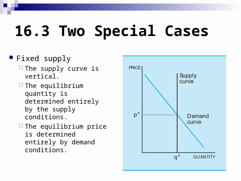
Fixed supply The supply curve is

vertical. The equilibrium quantity

is determined entirely by the supply conditions.

The equilibrium price is determined entirely by demand conditions.

16.3 Two Special Cases

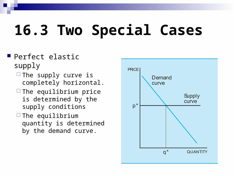
Perfect elastic supply The supply curve is

completely horizontal. The equilibrium price is

determined by the supply conditions

The equilibrium quantity is determined by the demand curve.

16.4 Inverse Demand and Supply Curves

Inverse supply function PS(q)

Inverse demand function PD(q)

Equilibrium is determined by the condition

PS(q)= PD(q)

EXAMPLE: Equilibrium with Linear Curves Suppose that both the demand and the supply

curves are linear:D(p)=a-bpS(p)=c+dp

The equilibrium price can be found by solving the following equation:

D(p)=a-bp=c+dp= S(p)

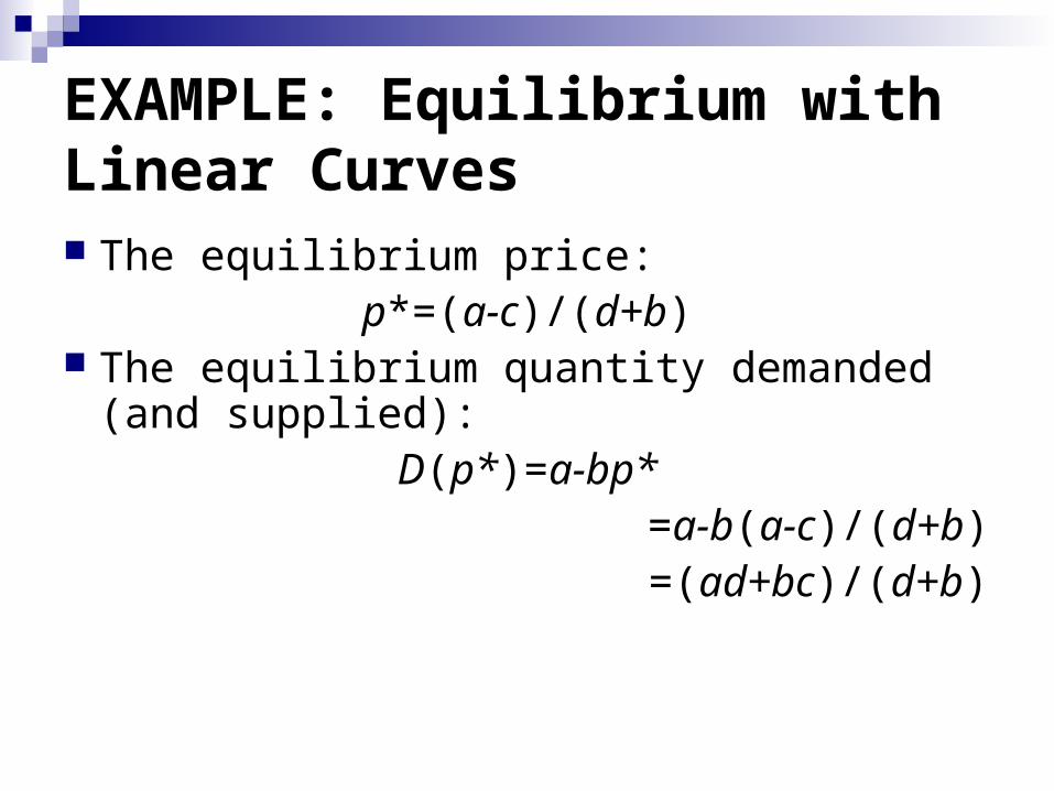
EXAMPLE: Equilibrium with Linear Curves The equilibrium price:

p*=(a-c)/(d+b) The equilibrium quantity demanded (and

supplied):D(p*)=a-bp*

=a-b(a-c)/(d+b) =(ad+bc)/(d+b)

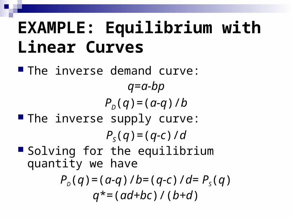
EXAMPLE: Equilibrium with Linear Curves The inverse demand curve:

q=a-bp

PD(q)=(a-q)/b The inverse supply curve:

PS(q)=(q-c)/d Solving for the equilibrium quantity we have

PD(q)=(a-q)/b=(q-c)/d= PS(q)q*=(ad+bc)/(b+d)

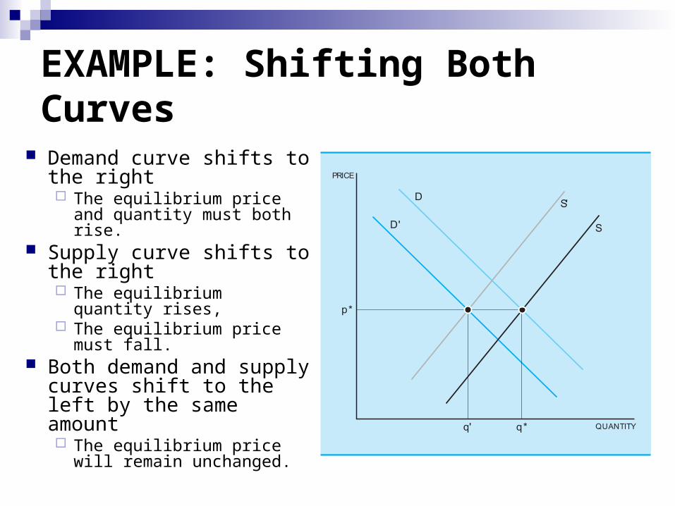
EXAMPLE: Shifting Both Curves

Demand curve shifts to the right The equilibrium price and

quantity must both rise. Supply curve shifts to the

right The equilibrium quantity

rises, The equilibrium price must

fall. Both demand and supply

curves shift to the left by the same amount The equilibrium price will

remain unchanged.

16.6 Taxes

A quantity tax: a tax levied per unit of quantity bought or sold.

PD=PS+t

The equilibrium quantity traded:

PD(q*)-t=PS(q*)

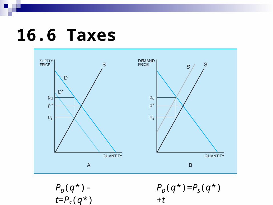
16.6 Taxes

PD(q*)-t=PS(q*) PD(q*)=PS(q*)+t

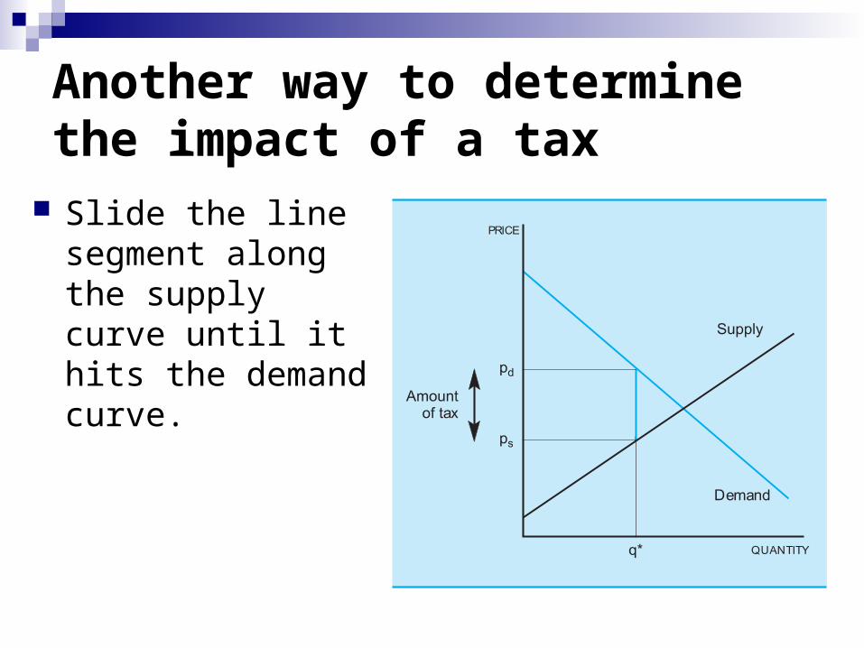
Another way to determine the impact of a tax

Slide the line segment along the supply curve until it hits the demand curve.

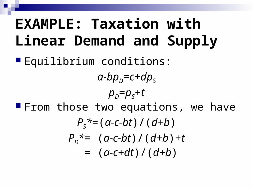
EXAMPLE: Taxation with Linear Demand and Supply Equilibrium conditions:

a-bpD=c+dpS

pD=pS+t From those two equations, we have

PS*=(a-c-bt)/(d+b)

PD*= (a-c-bt)/(d+b)+t= (a-c+dt)/(d+b)

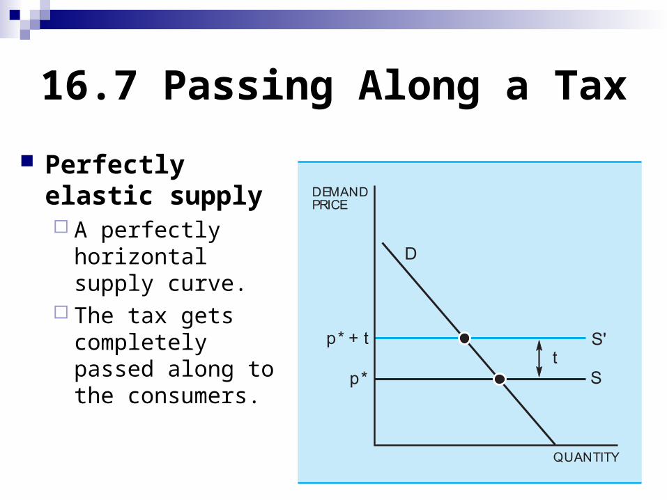
16.7 Passing Along a Tax

Perfectly elastic supply A perfectly horizontal

supply curve. The tax gets

completely passed along to the consumers.

16.7 Passing Along a Tax

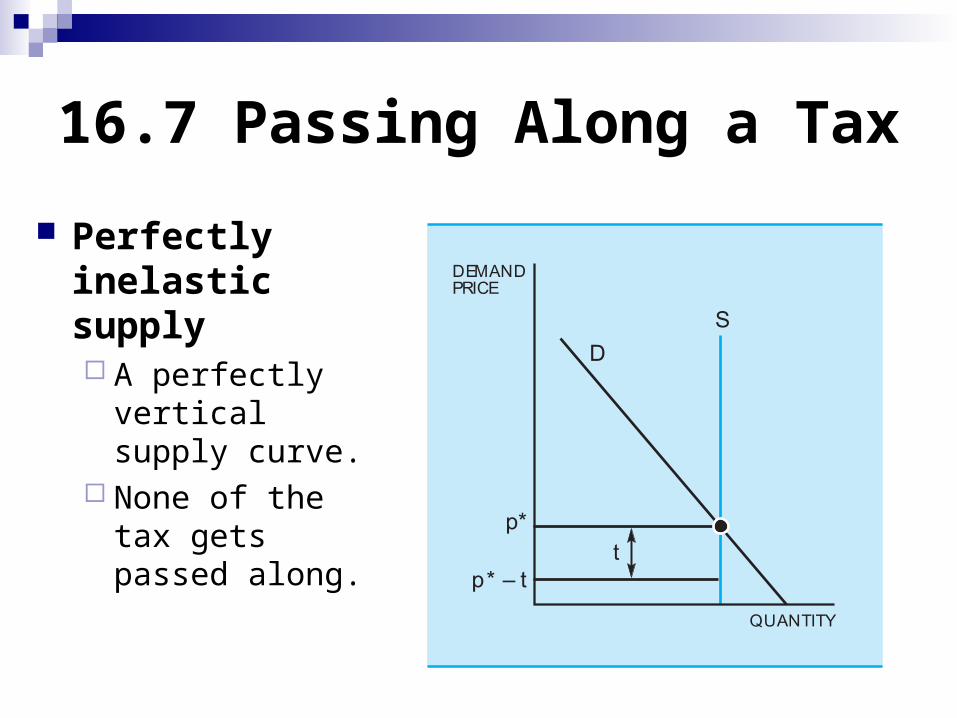
Perfectly inelastic supply A perfectly vertical

supply curve. None of the tax gets

passed along.

16.7 Passing Along a Tax

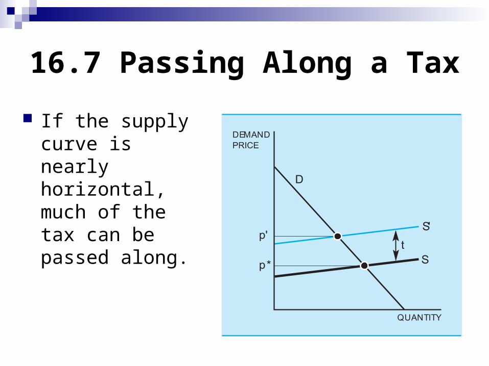
If the supply curve is nearly horizontal, much of the tax can be passed along.

16.7 Passing Along a Tax

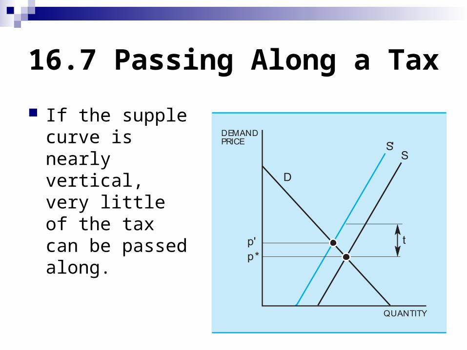
If the supple curve is nearly vertical, very little of the tax can be passed along.

16.8 The Deadweight Loss of a Tax

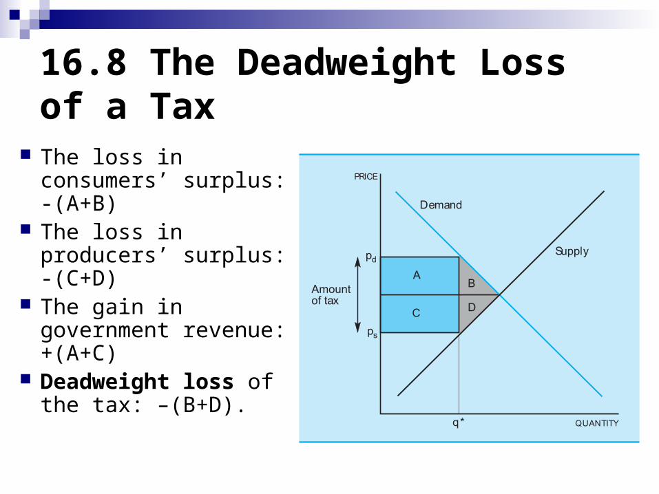
The loss of producers’ and consumers’ surpluses are net costs, and the tax revenue to the government is a net benefit, the total net cost of the tax is the algebraic sum of these areas: the loss in consumers’ surplus, -(A+B), the loss in producers’ surplus, -(C+D), and the gain in government revenue, +(A+C).

16.8 The Deadweight Loss of a Tax

The loss in consumers’ surplus: -(A+B)

The loss in producers’ surplus: -(C+D)

The gain in government revenue: +(A+C)

Deadweight loss of the tax: –(B+D).

EXAMPLE: The Market for Loans

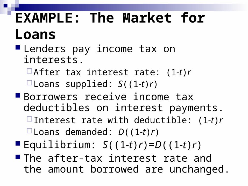
Lenders pay income tax on interests.After tax interest rate: (1-t)rLoans supplied: S((1-t)r)

Borrowers receive income tax deductibles on interest payments.Interest rate with deductible: (1-t)rLoans demanded: D((1-t)r)

Equilibrium: S((1-t)r)=D((1-t)r) The after-tax interest rate and the amount

borrowed are unchanged.

EXAMPLE: The Market for Loans

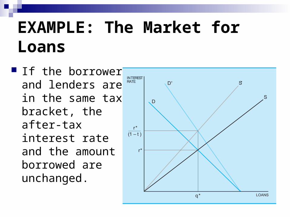
If the borrower and lenders are in the same tax bracket, the after-tax interest rate and the amount borrowed are unchanged.

16.9 Pareto Efficiency

Pareto Efficiency: there is no way to make any person better off without hurting anybody else.

16.9 Pareto Efficiency

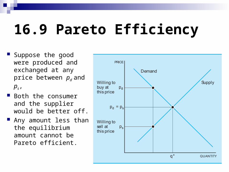
Suppose the good were produced and exchanged at any price between pd and ps,

Both the consumer and the supplier would be better off.

Any amount less than the equilibrium amount cannot be Pareto efficient.