Chapter 16

Complex Analysis

The term “complex analysis” refers to the calculus of complex-valued functions f(z)depending on a single complex variable z. On the surface, it may seem that this subjectshould merely be a simple reworking of standard real variable theory that you learnedin first year calculus. However, this naıve first impression could not be further from thetruth! Complex analysis is the culmination of a deep and far-ranging study of the fun-damental notions of complex differentiation and complex integration, and has an eleganceand beauty not found in the more familiar real arena. For instance, complex functionsare always analytic, meaning that they can be represented as convergent power series. Asan immediate consequence, a complex function automatically has an infinite number ofderivatives, and difficulties with degree of smoothness, strange discontinuities, delta func-tions, and other forms of pathological behavior of real functions never arise in the complexrealm.

The driving force behind many applications of complex analysis is the remarkable andprofound connection between harmonic functions (solutions of the Laplace equation) oftwo variables and complex functions. Namely, the real and imaginary parts of a complexanalytic function are automatically harmonic. In this manner, complex functions provide arich lode of new solutions to the two-dimensional Laplace equation to help solve boundaryvalue problems. One of the most useful practical consequences arises from the elementaryobservation that the composition of two complex functions is also a complex function. Weinterpret this operation as a complex changes of variables, also known as a conformal map-

ping since it preserves angles. Conformal mappings can be effectively used for constructingsolutions to the Laplace equation on complicated planar domains, and play a particularlyimportant role in the solution of physical problems.

Complex integration also enjoys many remarkable properties not found in its realsibling. Integrals of complex functions are similar to the line integrals of planar multi-variable calculus. The remarkable theorem due to Cauchy implies that complex integralsare generally path-independent — provided one pays proper attention to the complexsingularities of the integrand. In particular, an integral of a complex function around aclosed curve can be directly evaluated through the “calculus of residues”, which effectivelybypasses the Fundamental Theorem of Calculus. Surprisingly, the method of residues caneven be applied to evaluate certain types of definite real integrals.

In this chapter, we shall introduce the basic techniques and theorems in complexanalysis, paying particular attention to those aspects which are required to solve boundaryvalue problems associated with the planar Laplace and Poisson equations. Complex anal-ysis is an essential tool in a surprisingly broad range of applications, including fluid flow,

12/11/12 857 c© 2012 Peter J. Olver

elasticity, thermostatics, electrostatics, and, in mathematics, geometry, and even numbertheory. Indeed, the most famous unsolved problem in all of mathematics, the Riemann hy-pothesis, is a conjecture about a specific complex function that has profound consequencesfor the distribution of prime numbers†.

16.1. Complex Variables.

In this section we shall develop the basics of complex analysis — the calculus ofcomplex functions f(z). Here z = x + i y is a single complex variable and f : Ω → C isa complex-valued function defined on a domain z ∈ Ω ⊂ C in the complex plane. Beforediving into this material, you should first make sure you are familiar with the basics ofcomplex numbers, as discussed in Section 3.6.

Any complex function can be written as a complex combination

f(z) = f(x+ i y) = u(x, y) + i v(x, y), (16.1)

of two real functions u, v depending on two real variables x, y, called, respectively, its realand imaginary parts , and written

u(x, y) = Re f(z), and v(x, y) = Im f(z). (16.2)

For example, the monomial function f(z) = z3 is written as

z3 = (x+ i y)3 = (x3 − 3xy2) + i (3x2y − y3),

and so

Re z3 = x3 − 3xy2, Im z3 = 3x2y − y3.

We can identify C with the real, two-dimensional plane R2, so that the complexnumber z = x + i y ∈ C is identified with the real vector (x, y )

T ∈ R2. Based on thisidentification, we shall employ the standard terminology of planar vector calculus, e.g.,domain, curve, etc., without alteration; see Appendix A for details. In this manner, wemay regard a complex function as particular type of real vector field that maps

(xy

)∈ Ω ⊂ R2 to the vector v(x, y) =

(u(x, y)v(x, y)

)∈ R2. (16.3)

Not every real vector field qualifies as a complex function; the components u(x, y), v(x, y)must satisfy certain fairly stringent requirements, which can be found in Theorem 16.3below.

Many of the well-known functions appearing in real-variable calculus — polynomials,rational functions, exponentials, trigonometric functions, logarithms, and many others —have natural complex extensions. For example, complex polynomials

p(z) = an zn + an−1 z

n−1 + · · ·+ a1 z + a0 (16.4)

† Not to mention that a solution will net you a cool $1,000,000.00. For details on how to claimyour prize, check out the web site http://www.claymath.org.

12/11/12 858 c© 2012 Peter J. Olver

are complex linear combinations (meaning that the coefficients ak are allowed to be complexnumbers) of the basic monomial functions zk = (x+ i y)k. Similarly, we have already madesporadic use of complex exponentials such as

ez = ex+ i y = ex cos y + i ex sin y

for solving differential equations. Other examples will appear shortly.

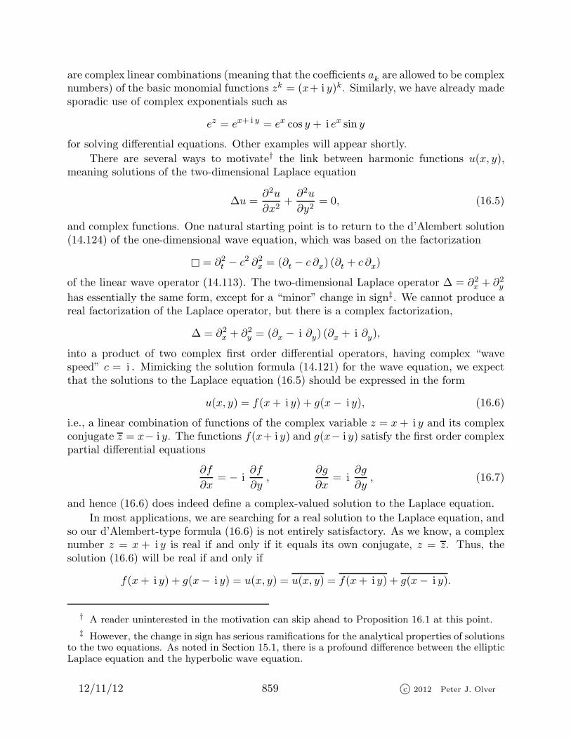
There are several ways to motivate† the link between harmonic functions u(x, y),meaning solutions of the two-dimensional Laplace equation

∆u =∂2u

∂x2+∂2u

∂y2= 0, (16.5)

and complex functions. One natural starting point is to return to the d’Alembert solution(14.124) of the one-dimensional wave equation, which was based on the factorization

= ∂2t − c2 ∂2x = (∂t − c ∂x) (∂t + c ∂x)

of the linear wave operator (14.113). The two-dimensional Laplace operator ∆ = ∂2x + ∂2yhas essentially the same form, except for a “minor” change in sign‡. We cannot produce areal factorization of the Laplace operator, but there is a complex factorization,

∆ = ∂2x + ∂2y = (∂x − i ∂y) (∂x + i ∂y),

into a product of two complex first order differential operators, having complex “wavespeed” c = i . Mimicking the solution formula (14.121) for the wave equation, we expectthat the solutions to the Laplace equation (16.5) should be expressed in the form

u(x, y) = f(x+ i y) + g(x− i y), (16.6)

i.e., a linear combination of functions of the complex variable z = x+ i y and its complexconjugate z = x− i y. The functions f(x+ i y) and g(x− i y) satisfy the first order complexpartial differential equations

∂f

∂x= − i

∂f

∂y,

∂g

∂x= i

∂g

∂y, (16.7)

and hence (16.6) does indeed define a complex-valued solution to the Laplace equation.

In most applications, we are searching for a real solution to the Laplace equation, andso our d’Alembert-type formula (16.6) is not entirely satisfactory. As we know, a complexnumber z = x + i y is real if and only if it equals its own conjugate, z = z. Thus, thesolution (16.6) will be real if and only if

f(x+ i y) + g(x− i y) = u(x, y) = u(x, y) = f(x+ i y) + g(x− i y).

† A reader uninterested in the motivation can skip ahead to Proposition 16.1 at this point.

‡ However, the change in sign has serious ramifications for the analytical properties of solutionsto the two equations. As noted in Section 15.1, there is a profound difference between the ellipticLaplace equation and the hyperbolic wave equation.

12/11/12 859 c© 2012 Peter J. Olver

Now, the complex conjugation operation switches x+ i y and x− i y, and so we expect thefirst term f(x+ i y) to be a function of x− i y, while the second term g(x− i y) will be afunction of x+ i y. Therefore§, to equate the two sides of this equation, we should require

g(x− i y) = f(x+ i y),

and sou(x, y) = f(x+ i y) + f(x+ i y) = 2 Re f(x+ i y).

Dropping the inessential factor of 2, we conclude that a real solution to the two-dimensionalLaplace equation can be written as the real part of a complex function. A direct proof ofthe following key result will appear below.

Proposition 16.1. If f(z) is a complex function, then its real part

u(x, y) = Re f(x+ i y) (16.8)

is a harmonic function.

The imaginary part of a complex function is also harmonic. This is because

Im f(z) = Re (− i f(z))

is the real part of the complex function

− i f(z) = − i [u(x, y) + i v(x, y)] = v(x, y)− i u(x, y).

Therefore, if f(z) is any complex function, we can write it as a complex combination

f(z) = f(x+ i y) = u(x, y) + i v(x, y),

of two real harmonic functions: u(x, y) = Re f(z) and v(x, y) = Im f(z).

Before delving into the many remarkable properties of complex functions, let us lookat some of the most basic examples. In each case, the reader can directly check thatthe harmonic functions given as the real and imaginary parts of the complex function areindeed solutions to the Laplace equation.

Examples of Complex Functions

(a) Harmonic Polynomials : The simplest examples of complex functions are polynomi-als. Any polynomial is a complex linear combinations, as in (16.4), of the basic complexmonomials

zn = (x+ i y)n = un(x, y) + i vn(x, y). (16.9)

The real and imaginary parts of a complex polynomial are known as harmonic polynomials ,and we list the first few below. The general formula for the basic harmonic polynomials

§ We are ignoring the fact that f and g are not quite uniquely determined since one can addand subtract a constant from them. This does not affect the argument in any significant way.

12/11/12 860 c© 2012 Peter J. Olver

Re z2 Re z3

Im z2 Im z3

Figure 16.1. Real and Imaginary Parts of z2 and z3.

un(x, y) and vn(x, y) is easily found by applying the binomial theorem to expand (16.9),as in Exercise .

Harmonic Polynomials

n zn un(x, y) vn(x, y)

0 1 1 0

1 x+ i y x y

2 (x2 − y2) + 2 i xy x2 − y2 2xy

3 (x3 − 3xy2) + i (3x2y − y3) x3 − 3xy2 3x2y − y3

4 (x4 − 6x2y2 + y4) + i (4x3y − 4xy3) x4 − 6x2y2 + y4 4x3y − 4xy3

......

......

We have, in fact, already encountered these polynomial solutions to the Laplace equa-tion. If we write

z = r e i θ, (16.10)

where

r = | z | =√x2 + y2, θ = ph z = tan−1 y

x,

12/11/12 861 c© 2012 Peter J. Olver

Re1z Im

1z

Figure 16.2. Real and Imaginary Parts of f(z) =1z .

are the usual polar coordinates (modulus and phase) of z = x + i y, then Euler’s for-mula (3.84) yields

zn = rn e inθ = rn cosnθ + i rn sinnθ,

and so

un = rn cosnθ, vn = rn sinnθ.

Therefore, the harmonic polynomials are just the polar coordinate separablesolutions(15.38) to the Laplace equation. In Figure 16.1 we plot† the real and imaginary partsof the monomials z2 and z3.

(b) Rational Functions : Ratios

f(z) =p(z)

q(z)(16.11)

of complex polynomials provide a large variety of harmonic functions. The simplest caseis

1

z=

z

z z=

z

| z |2 =x

x2 + y2− i

y

x2 + y2. (16.12)

Its real and imaginary parts are graphed in Figure 16.2. Note that these functions havean interesting singularity at the origin x = y = 0, but are harmonic everywhere else.

A slightly more complicated example is the function

f(z) =z − 1

z + 1. (16.13)

† Graphing a complex function f :C → C is problematic. The identification (16.3) of f with

a real vector-valued function f :R2→ R

2 implies that four real dimensions are needed to displayits complete graph.

12/11/12 862 c© 2012 Peter J. Olver

To write out (16.13) in real form, we multiply and divide by the complex conjugate of thedenominator, leading to

f(z) =z − 1

z + 1=

(z − 1)(z + 1)

(z + 1)(z + 1)=

| z |2 + z − z − 1

| z + 1 |2 =x2 + y2 − 1

(x+ 1)2 + y2+ i

2y

(x+ 1)2 + y2.

(16.14)This manipulation can always be used to find the real and imaginary parts of generalrational functions.

(c) Complex Exponentials : Euler’s formula

ez = ex cos y + i ex sin y (16.15)

for the complex exponential, cf. (3.84), yields two important harmonic functions: ex cos yand ex sin y, which are graphed in Figure 3.8. More generally, writing out ecz for a complexconstant c = a+ i b produces the complex exponential function

ecz = eax−by cos(bx+ ay) + i eax−by sin(bx+ ay). (16.16)

Its real and imaginary parts are harmonic functions for arbitrary a, b ∈ R. Some of thesewere found by applying the separation of variables method in Cartesian coordinates; seethe table in Section 15.2.

(d) Complex Trigonometric Functions : The complex trigonometric functions are de-fined in terms of the complex exponential by adapting our earlier formulae (3.86):

cos z =e i z + e− i z

2= cosx cosh y − i sinx sinh y,

sin z =e i z − e− i z

2 i= sinx cosh y + i cosx sinh y.

(16.17)

The resulting harmonic functions are products of trigonometric and hyperbolic functions.They can all be written as linear combinations of the harmonic functions (16.16) derivedfrom the complex exponential. Note that when z = x is real, so y = 0, these functionsreduce to the usual real trigonometric functions cosx and sinx.

(e) Complex Logarithm: In a similar fashion, the complex logarithm log z is a complexextension of the usual real natural (i.e., base e) logarithm. In terms of polar coordinates(16.10), the complex logarithm has the form

log z = log(r e i θ) = log r + log e i θ = log r + i θ, (16.18)

Thus, the logarithm of a complex number has real part

Re (log z) = log r = log | z | = 12 log(x2 + y2),

which is a well-defined harmonic function on all of R2 except for a logarithmic singularityat the origin x = y = 0. It is, in fact, the logarithmic potential corresponding to a deltafunction forcing concentrated at the origin that played a key role in our construction ofthe Green’s function for the Poisson equation in Section 15.3.

The imaginary partIm (log z) = θ = ph z

12/11/12 863 c© 2012 Peter J. Olver

Re (log z) = log | z | Im (log z) = ph z

Figure 16.3. Real and Imaginary Parts of log z.

of the complex logarithm is the phase (argument) or polar angle of z. The phase is alsonot defined at the origin x = y = 0. Moreover, it is a multi-valued harmonic functionelsewhere, since it is only specified up to integer multiples of 2π. Thus, a given nonzerocomplex number z 6= 0 has an infinite number of possible values for its phase, and hence aninfinite number of possible complex logarithms log z, each differing by an integer multipleof 2π i , reflecting the fact that e2π i = 1. In particular, if z = x > 0 is real and positive,then log z = log x agrees with the real logarithm, provided we choose the angle ph z = 0.Alternative choices for the phase include an integer multiple of 2π i , and so ordinary real,positive numbers x > 0 also have complex logarithms! On the other hand, if z = x < 0 isreal and negative, then log z = log | x |+ (2k + 1)π i is complex no matter which value ofph z is chosen. (This explains why we didn’t attempt to define the logarithm of a negativenumber in first year calculus!) As the point z circles around the origin in a counter-clockwise direction, Im log z = ph z = θ increases by 2π. Thus, its graph can be likened toa parking ramp with infinitely many levels, spiraling ever upwards as one circumabulatesthe origin; Figure 16.3 attempts to sketch it. For the complex logarithm, the origin is atype of singularity known as a logarithmic branch point , the “branches” referring to theinfinite number of possible values that can be assigned to log z at any nonzero point.

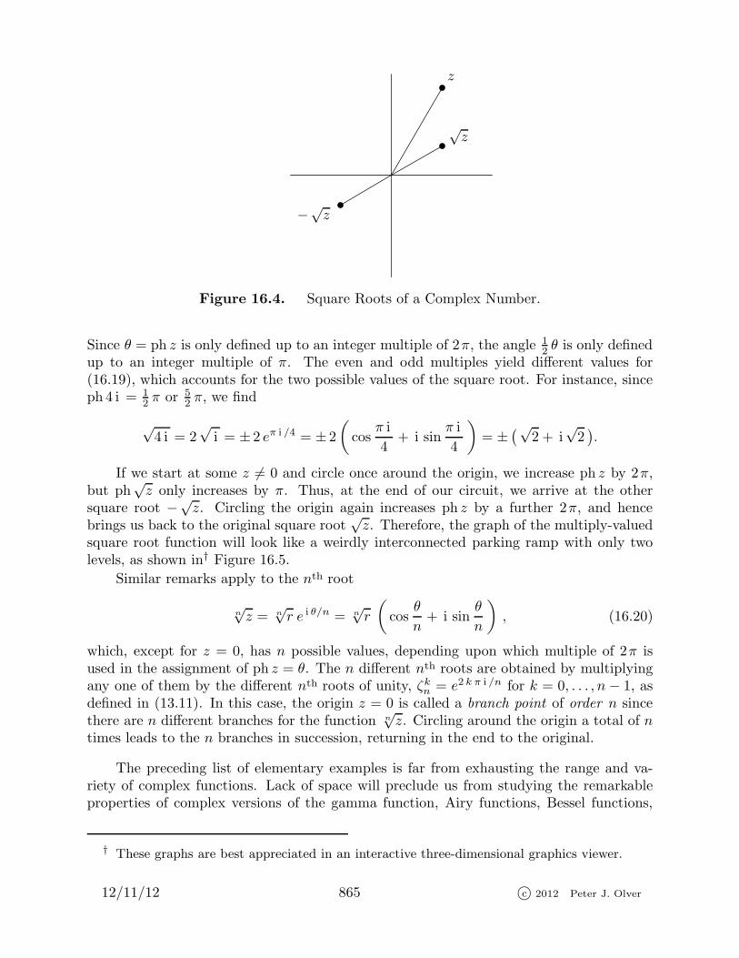
(f ) Roots and Fractional Powers : A similar branching phenomenon occurs with thefractional powers and roots of complex numbers. The simplest case is the square rootfunction

√z. Every nonzero complex number z 6= 0 has two different possible square

roots:√z and −√

z. As illustrated in Figure 16.4, the two square roots lie on oppositesides of the origin, and are obtained by multiplying by −1. Writing z = r e i θ in polarcoordinates, we see that

√z =

√r e i θ =

√r e i θ/2 =

√r

(cos

θ

2+ i sin

θ

2

), (16.19)

i.e., we take the square root of the modulus and halve the phase:

∣∣√z∣∣ =

√| z | =

√r , ph

√z = 1

2 ph z = 12 θ.

12/11/12 864 c© 2012 Peter J. Olver

z

√z

−√z

Figure 16.4. Square Roots of a Complex Number.

Since θ = ph z is only defined up to an integer multiple of 2π, the angle 12 θ is only defined

up to an integer multiple of π. The even and odd multiples yield different values for(16.19), which accounts for the two possible values of the square root. For instance, sinceph 4 i = 1

2π or 5

2π, we find

√4 i = 2

√i = ± 2 eπ i /4 = ± 2

(cos

π i

4+ i sin

π i

4

)= ±

(√2 + i

√2).

If we start at some z 6= 0 and circle once around the origin, we increase ph z by 2π,but ph

√z only increases by π. Thus, at the end of our circuit, we arrive at the other

square root −√z. Circling the origin again increases ph z by a further 2π, and hence

brings us back to the original square root√z. Therefore, the graph of the multiply-valued

square root function will look like a weirdly interconnected parking ramp with only twolevels, as shown in† Figure 16.5.

Similar remarks apply to the nth root

n√z = n

√r e i θ/n = n

√r

(cos

θ

n+ i sin

θ

n

), (16.20)

which, except for z = 0, has n possible values, depending upon which multiple of 2π isused in the assignment of ph z = θ. The n different nth roots are obtained by multiplyingany one of them by the different nth roots of unity, ζkn = e2 k π i /n for k = 0, . . . , n − 1, asdefined in (13.11). In this case, the origin z = 0 is called a branch point of order n sincethere are n different branches for the function n

√z. Circling around the origin a total of n

times leads to the n branches in succession, returning in the end to the original.

The preceding list of elementary examples is far from exhausting the range and va-riety of complex functions. Lack of space will preclude us from studying the remarkableproperties of complex versions of the gamma function, Airy functions, Bessel functions,

† These graphs are best appreciated in an interactive three-dimensional graphics viewer.

12/11/12 865 c© 2012 Peter J. Olver

Figure 16.5. Real and Imaginary Parts of√z .

and Legendre functions that appear in Appendix C, as well as elliptic functions, the Rie-mann zeta function, modular functions, and many, many other important and fascinatingfunctions arising in complex analysis and its manifold applications; see [179, 190].

16.2. Complex Differentiation.

The bedrock of complex function theory is the notion of the complex derivative. Com-plex differentiation is defined in the same manner as the usual calculus limit definition ofthe derivative of a real function. Yet, despite a superficial similarity, complex differenti-ation is profoundly different, and displays an elegance and depth not shared by its realprogenitor.

Definition 16.2. A complex function f(z) is differentiable at a point z ∈ C if andonly if the limiting difference quotient exists:

f ′(z) = limw→ z

f(w)− f(z)

w − z. (16.21)

The key feature of this definition is that the limiting value f ′(z) of the differencequotient must be independent of how w converges to z. On the real line, there are onlytwo directions to approach a limiting point — either from the left or from the right. Theselead to the concepts of left and right handed derivatives and their equality is required forthe existence of the usual derivative of a real function. In the complex plane, there arean infinite variety of directions to approach the point z, and the definition requires thatall of these “directional derivatives” must agree. This is the reason for the more severerestrictions on complex derivatives, and, in consequence, the source of their remarkableproperties.

12/11/12 866 c© 2012 Peter J. Olver

z z + h

z + i k

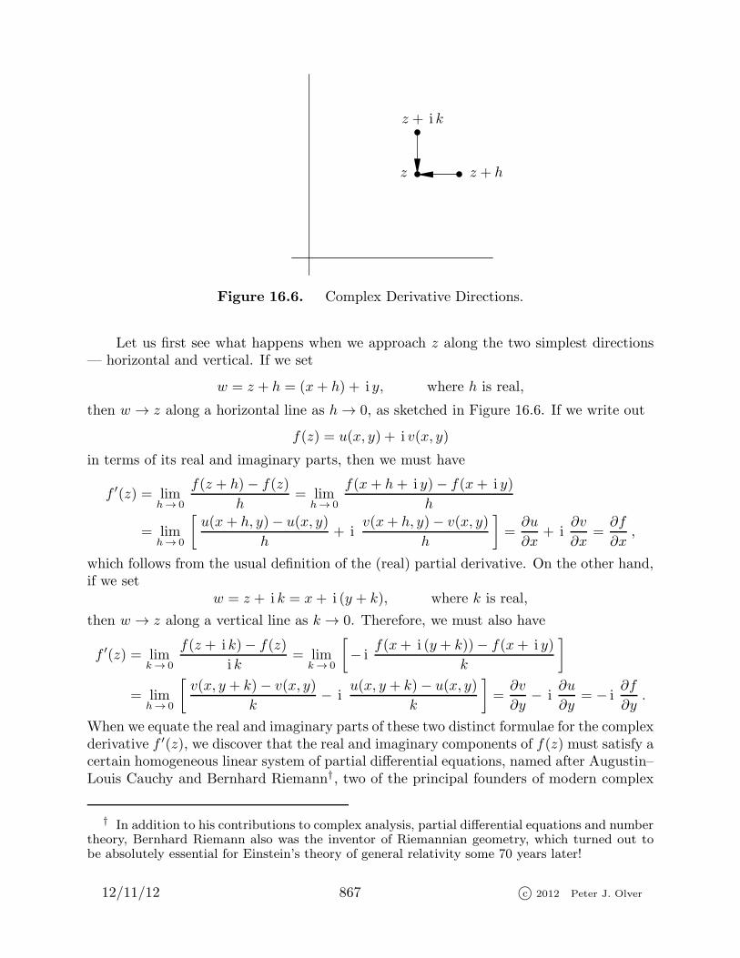
Figure 16.6. Complex Derivative Directions.

Let us first see what happens when we approach z along the two simplest directions— horizontal and vertical. If we set

w = z + h = (x+ h) + i y, where h is real,

then w → z along a horizontal line as h→ 0, as sketched in Figure 16.6. If we write out

f(z) = u(x, y) + i v(x, y)

in terms of its real and imaginary parts, then we must have

f ′(z) = limh→ 0

f(z + h)− f(z)

h= lim

h→ 0

f(x+ h+ i y)− f(x+ i y)

h

= limh→ 0

[u(x+ h, y)− u(x, y)

h+ i

v(x+ h, y)− v(x, y)

h

]=∂u

∂x+ i

∂v

∂x=∂f

∂x,

which follows from the usual definition of the (real) partial derivative. On the other hand,if we set

w = z + i k = x+ i (y + k), where k is real,

then w → z along a vertical line as k → 0. Therefore, we must also have

f ′(z) = limk→ 0

f(z + i k)− f(z)

i k= lim

k→ 0

[− i

f(x+ i (y + k))− f(x+ i y)

k

]

= limh→ 0

[v(x, y + k)− v(x, y)

k− i

u(x, y + k)− u(x, y)

k

]=∂v

∂y− i

∂u

∂y= − i

∂f

∂y.

When we equate the real and imaginary parts of these two distinct formulae for the complexderivative f ′(z), we discover that the real and imaginary components of f(z) must satisfy acertain homogeneous linear system of partial differential equations, named after Augustin–Louis Cauchy and Bernhard Riemann†, two of the principal founders of modern complex

† In addition to his contributions to complex analysis, partial differential equations and numbertheory, Bernhard Riemann also was the inventor of Riemannian geometry, which turned out tobe absolutely essential for Einstein’s theory of general relativity some 70 years later!

12/11/12 867 c© 2012 Peter J. Olver

analysis.

Theorem 16.3. A function f(z) = u(x, y) + i v(x, y), where z = x + i y, has a

complex derivative f ′(z) if and only if its real and imaginary parts are continuously differ-

entiable and satisfy the Cauchy–Riemann equations

∂u

∂x=∂v

∂y,

∂u

∂y= − ∂v

∂x. (16.22)

In this case, the complex derivative of f(z) is equal to any of the following expressions:

f ′(z) =∂f

∂x=∂u

∂x+ i

∂v

∂x= − i

∂f

∂y=∂v

∂y− i

∂u

∂y. (16.23)

The proof of the converse — that any function whose real and imaginary componentssatisfy the Cauchy–Riemann equations is differentiable — will be omitted, but can befound in any basic text on complex analysis, e.g., [4, 160].

Remark : It is worth pointing out that equation (16.23) tells us that f satisfies ∂f/∂x =− i ∂f/∂y, which, reassuringly, agrees with the first equation in (16.7).

Example 16.4. Consider the elementary function

z3 = (x3 − 3xy2) + i (3x2y − y3).

Its real part u = x3−3xy2 and imaginary part v = 3x2y−y3 satisfy the Cauchy–Riemannequations (16.22), since

∂u

∂x= 3x2 − 3y2 =

∂v

∂y,

∂u

∂y= −6xy = − ∂v

∂x.

Theorem 16.3 implies that f(z) = z3 is complex differentiable. Not surprisingly, its deriva-tive turns out to be

f ′(z) = 3z2 = (3x2 − 3y2) + i (6xy) =∂u

∂x+ i

∂v

∂x=∂v

∂y− i

∂u

∂y.

Fortunately, the complex derivative obeys all of the usual rules that you learned inreal-variable calculus. For example,

d

dzzn = n zn−1,

d

dzecz = c ecz,

d

dzlog z =

1

z, (16.24)

and so on. The power n can even be non-integral or, in view of the identity zn = en log z,complex, while c is any complex constant. The exponential formulae (16.17) for the com-plex trigonometric functions implies that they also satisfy the standard rules

d

dzcos z = − sin z,

d

dzsin z = cos z. (16.25)

The formulae for differentiating sums, products, ratios, inverses, and compositions of com-plex functions are all identical to their real counterparts. Thus, thankfully, you don’t needto learn any new rules for performing complex differentiation!

12/11/12 868 c© 2012 Peter J. Olver

Remark : There are many examples of seemingly reasonable functions which do not

have a complex derivative. The simplest is the complex conjugate function

f(z) = z = x− i y.

Its real and imaginary parts do not satisfy the Cauchy–Riemann equations, and hence zdoes not have a complex derivative. More generally, any function f(x, y) = h(z, z) thatexplicitly depends on the complex conjugate variable z is not complex-differentiable.

Power Series and Analyticity

The most remarkable feature of complex analysis, which distinguishes it from realfunction theory, is that the existence of one complex derivative automatically implies theexistence of infinitely many! All complex functions f(z) are infinitely differentiable and, infact, analytic where defined. The reason for this surprising and profound fact will, however,not become evident until we learn the basics of complex integration in Section 16.5. Inthis section, we shall take analyticity as a given, and investigate some of its principalconsequences.

Definition 16.5. A complex function f(z) is called analytic at a point z0 if it has apower series expansion

f(z) = a0 + a1(z − z0) + a2(z − z0)2 + a3(z − z0)

3 + · · · =

∞∑

n=0

an (z − z0)n , (16.26)

which converges for all z sufficiently close to z0.

Typically, the standard ratio or root tests for convergence of (real) series that youlearned in ordinary calculus, [9, 171], can be applied to determine where a given (complex)power series converges. We note that if f(z) and g(z) are analytic at a point z0, so is theirsum f(z) + g(z), product f(z) g(z) and, provided g(z0) 6= 0, ratio f(z)/g(z).

Example 16.6. All of the real power series found in elementary calculus carry overto the complex versions of the functions. For example,

ez = 1 + z + 12 z

2 + 16 z

3 + · · · =

∞∑

n=0

zn

n!(16.27)

is the Taylor series for the exponential function based at z0 = 0. A simple applicationof the ratio test proves that the series converges for all z. On the other hand, the powerseries

1

z2 + 1= 1− z2 + z4 − z6 + · · · =

∞∑

k=0

(−1)k z2k , (16.28)

converges inside the unit disk, where | z | < 1, and diverges outside, where | z | > 1. Again,convergence is established through the ratio test. The ratio test is inconclusive when| z | = 1, and we shall leave the more delicate question of precisely where on the unit diskthis complex series converges to a more advanced treatment, e.g., [4].

12/11/12 869 c© 2012 Peter J. Olver

In general, there are three possible options for the domain of convergence of a complexpower series (16.26):

(a) The series converges for all z.

(b) The series converges inside a disk | z − z0 | < ρ of radius ρ > 0 centered at z0 anddiverges for all | z − z0 | > ρ outside the disk. The series may converge at some(but not all) of the points on the boundary of the disk where | z − z0 | = ρ.

(c) The series only converges, trivially, at z = z0.

The number ρ is known as the radius of convergence of the series. In case (a), we sayρ = ∞, while in case (c), ρ = 0, and the series does not represent an analytic function. Anexample with ρ = 0 is the power series

∑n! zn. In the intermediate case (b), determining

precisely where on the boundary of the convergence disk the power series converges is quitedelicate, and will not be pursued here. The proof of this result can be found in Exercise; see also [4, 95] for further details.

Remarkably, the radius of convergence for the power series of a known analytic functionf(z) can be determined by inspection, without recourse to any fancy convergence tests!Namely, ρ is equal to the distance from z0 to the nearest singularity of f(z), meaning apoint where the function fails to be analytic. This explains why the Taylor series of ez

converges everywhere, while that of (z2 + 1)−1 only converges inside the unit disk. Indeedez is analytic for all z and has no singularities; therefore the radius of convergence of itspower series — centered at any point z0 — is equal to ρ = ∞. On the other hand, thefunction

f(z) =1

z2 + 1=

1

(z + i )(z − i )

has singularities at z = ± i , and so the series (16.28) has radius of convergence ρ = 1,which is the distance from z0 = 0 to the singularities. Thus, the extension of the theoryof power series to the complex plane serves to explain the apparent mystery of why, asa real function, (1 + x2)−1 is well-defined and analytic for all real x, but its power seriesonly converges on the interval (−1, 1). It is the complex singularities that prevent itsconvergence when | x | > 1. If we expand (z2 + 1)−1 in a power series at some other point,say z0 = 1 + 2 i , then we need to determine which singularity is closest. We compute| i − z0 | = | −1− i | =

√2, while | − i − z0 | = | −1− 3 i | =

√10, and so the radius of

convergence ρ =√2 is the smaller. Thus we can determine the radius of convergence

without any explicit formula for its (rather complicated) Taylor expansion at z0 = 1+ 2 i .

There are, in fact, only three possible types of singularities of a complex function f(z):

(i) Pole. A singular point z = z0 is called a pole of order n > 0 if and only if

f(z) =h(z)

(z − z0)n, (16.29)

where h(z) is analytic at z = z0 and h(z0) 6= 0. The simplest example of such afunction is f(z) = a (z − z0)

−n for a 6= 0 a complex constant.

(ii) Branch point . We have already encountered the two basic types: algebraic branch

points , such as the function n√z at z0 = 0, and logarithmic branch points such as

log z at z0 = 0. The degree of the branch point is n in the first case and ∞ in thesecond.

12/11/12 870 c© 2012 Peter J. Olver

(iii) Essential singularity . By definition, a singularity is essential if it is not a pole or abranch point. The simplest example is the essential singularity at z0 = 0 of thefunction e1/z. Details are left as an Exercise .

Example 16.7. The complex function

f(z) =ez

z3 − z2 − 5z − 3=

ez

(z − 3)(z + 1)2

is analytic everywhere except for singularities at the points z = 3 and z = −1, where itsdenominator vanishes. Since

f(z) =h1(z)

z − 3, where h1(z) =

ez

(z + 1)2

is analytic at z = 3 and h1(3) =116 e

3 6= 0, we see that z = 3 is a simple (order 1) pole forf(z). Similarly,

f(z) =h2(z)

(z + 1)2, where h2(z) =

ez

z − 3

is analytic at z = −1 with h2(−1) = − 14e−1 6= 0, we see that the point z = −1 is a double

(order 2) pole.

A complicated complex function can have a variety of singularities. For example, thefunction

f(z) =3√z + 2 e−1/z

z2 + 1(16.30)

has simple poles at z = ± i , a branch point of degree 3 at z = −2, and an essentialsingularity at z = 0.

As in the real case, and unlike Fourier series, convergent power series can always berepeatedly term-wise differentiated. Therefore, given the convergent series (16.26), we havethe corresponding series

f ′(z) = a1 + 2a2(z − z0) + 3a3(z − z0)2 + 4a4(z − z0)

3 + · · · =∞∑

n=0

(n+ 1)an+1(z − z0)n,

f ′′(z) = 2a2 + 6a3(z − z0) + 12a4(z − z0)2 + 20a5(z − z0)

3 + · · ·

=

∞∑

n=0

(n+ 1)(n+ 2)an+2(z − z0)n, (16.31)

and so on, for its derivatives. The proof that the differentiated series have the sameradius of convergence can be found in [4, 160]. As a consequence, we deduce the followingimportant result.

Theorem 16.8. Any analytic function is infinitely differentiable.

12/11/12 871 c© 2012 Peter J. Olver

ρ

z0

Ω

Figure 16.7. Radius of Convergence.

In particular, when we substitute z = z0 into the successively differentiated series, wediscover that

a0 = f(z0), a1 = f ′(z0), a2 = 12 f

′′(z0),

and, in general,

an =f (n)(z)

n!. (16.32)

Therefore, a convergent power series (16.26) is, inevitably, the usual Taylor series

f(z) =∞∑

n=0

f (n)(z0)

n!(z − z0)

n , (16.33)

for the function f(z) at the point z0.

Let us conclude this section by summarizing the fundamental theorem that character-izes complex functions. A complete, rigorous proof relies on complex integration theory,which is the topic of Section 16.5.

Theorem 16.9. Let Ω ⊂ C be an open set. The following properties are equivalent:

(a) The function f(z) has a continuous complex derivative f ′(z) for all z ∈ Ω.

(b) The real and imaginary parts of f(z) have continuous partial derivatives and satisfy

the Cauchy–Riemann equations (16.22) in Ω.

(c) The function f(z) is analytic for all z ∈ Ω, and so is infinitely differentiable and has a

convergent power series expansion at each point z0 ∈ Ω. The radius of convergenceρ is at least as large as the distance from z0 to the boundary ∂Ω; see Figure 16.7.

From now on, we reserve the term complex function to signifiy one that satisfies theconditions of Theorem 16.9. Sometimes one of the equivalent adjectives “analytic” or“holomorphic”, is added for emphasis. From now on, all complex functions are assumed tobe analytic everywhere on their domain of definition, except, possibly, at certain isolatedsingularities.

12/11/12 872 c© 2012 Peter J. Olver

16.3. Harmonic Functions.

We began this section by motivating the analysis of complex functions through appli-cations to the solution of the two-dimensional Laplace equation. Let us now formalize theprecise relationship between the two subjects.

Theorem 16.10. If f(z) = u(x, y)+ i v(x, y) is any complex analytic function, then

its real and imaginary parts, u(x, y), v(x, y), are both harmonic functions.

Proof : Differentiating† the Cauchy–Riemann equations (16.22), and invoking theequality of mixed partial derivatives, we find that

∂2u

∂x2=

∂

∂x

(∂u

∂x

)=

∂

∂x

(∂v

∂y

)=

∂2v

∂x ∂y=

∂

∂y

(∂v

∂x

)=

∂

∂y

(− ∂u

∂y

)= − ∂2u

∂y2.

Therefore, u is a solution to the Laplace equation uxx + uyy = 0. The proof for v issimilar. Q.E.D.

Thus, every complex function gives rise to two harmonic functions. It is, of course, ofinterest to know whether we can invert this procedure. Given a harmonic function u(x, y),does there exist a harmonic function v(x, y) such that f = u + i v is a complex analyticfunction? If so, the harmonic function v(x, y) is known as a harmonic conjugate to u. Theharmonic conjugate is found by solving the Cauchy–Riemann equations

∂v

∂x= − ∂u

∂y,

∂v

∂y=∂u

∂x, (16.34)

which, for a prescribed function u(x, y), constitutes an inhomogeneous linear system ofpartial differential equations for v(x, y). As such, it is usually not hard to solve, as thefollowing example illustrates.

Example 16.11. As the reader can verify, the harmonic polynomial

u(x, y) = x3 − 3x2y − 3xy2 + y3

satisfies the Laplace equation everywhere. To find a harmonic conjugate, we solve theCauchy–Riemann equations (16.34). First of all,

∂v

∂x= − ∂u

∂y= 3x2 + 6xy − 3y2,

and hence, by direct integration with respect to x,

v(x, y) = x3 + 3x2y − 3xy2 + h(y),

where h(y) — the “constant of integration” — is a function of y alone. To determine h wesubstitute our formula into the second Cauchy–Riemann equation:

3x2 − 6xy + h′(y) =∂v

∂y=∂u

∂x= 3x2 − 6xy − 3y2.

† Theorem 16.9 allows us to differentiate u and v as often as desired.

12/11/12 873 c© 2012 Peter J. Olver

Therefore, h′(y) = −3y2, and so h(y) = −y3 + c, where c is a real constant. We concludethat every harmonic conjugate to u(x, y) has the form

v(x, y) = x3 + 3x2y − 3xy2 − y3 + c.

Note that the corresponding complex function

u(x, y) + i v(x, y) = (x3 − 3x2y − 3xy2 + y3) + i (x3 + 3x2y − 3xy2 − y3 + c)

= (1− i )z3 + c

turns out to be a complex cubic polynomial.

Remark : On a connected domain, all harmonic conjugates to a given function u(x, y)only differ by a constant: v(x, y) = v(x, y) + c; see Exercise .

Although most harmonic functions have harmonic conjugates, unfortunately this isnot always the case. Interestingly, the existence or non-existence of a harmonic conjugatecan depend on the underlying geometry of the domain of definition of the function. If thedomain is simply-connected, and so contains no holes, then one can always find a harmonicconjugate. Otherwise, if the domain of definition Ω of our harmonic function u(x, y) is notsimply-connected, then there may not exist a single-valued harmonic conjugate v(x, y) toserve as the imaginary part of a complex function f(z).

Example 16.12. The simplest example where the latter possibility occurs is thelogarithmic potential

u(x, y) = log r = 12 log(x2 + y2).

This function is harmonic on the non-simply-connected domain Ω = C \ 0, but it isnot the real part of any single-valued complex function. Indeed, according to (16.18), thelogarithmic potential is the real part of the multiply-valued complex logarithm log z, andso its harmonic conjugate† is ph z = θ, which cannot be consistently and continuouslydefined on all of Ω. On the other hand, restricting z to a simply connected subdomainΩ 6∋ 0 allows us to select a continuous, single-valued branch of the angle θ = ph z, and solog r does have a genuine harmonic conjugate on Ω.

The harmonic functionu(x, y) =

x

x2 + y2

is also defined on the same non-simply-connected domain Ω = C \ 0 with a singularityat x = y = 0. In this case, there is a single valued harmonic conjugate, namely

v(x, y) = − y

x2 + y2,

which is defined on all of Ω. Indeed, according to (16.12), these functions define the realand imaginary parts of the complex function u+ i v = 1/z. Alternatively, one can directlycheck that they satisfy the Cauchy–Riemann equations (16.22).

† We can, by a previous remark, add in any constant to the harmonic conjugate, but this doesnot affect the subsequent argument.

12/11/12 874 c© 2012 Peter J. Olver

Remark : On the “punctured” plane Ω = C \ 0, the logarithmic potential is, in asense, the only counterexample that prevents a harmonic conjugate from being constructed.It can be shown, [XC], that if u(x, y) is a harmonic function defined on a punctureddisk ΩR =

0 < | z | < R

, where 0 < R ≤ ∞, then there exists a constant c such

that u(x, y) = u(x, y) − c log r is also harmonic and possess a single-valued harmonic

conjugate v(x, y). As a result, the function f = u + i v is analytic on all of ΩR, andso our original function u(x, y) is the real part of the multiply-valued analytic function

f(z) = f(z) + c log z. We shall use this fact in our later analysis of airfoils.

Theorem 16.13. Every harmonic function u(x, y) defined on a simply-connected

domain Ω is the real part of a complex valued function f(z) = u(x, y) + i v(x, y) which is

defined for all z = x+ i y ∈ Ω.

Proof : We first rewrite the Cauchy–Riemann equations (16.34) in vectorial form asan equation for the gradient of v:

∇v = ∇⊥u, where ∇⊥u =

(−uyux

)(16.35)

is the vector field that is everywhere orthogonal to the gradient of u and of the same length:

∇u · ∇⊥u = 0, ‖∇⊥u ‖ = ‖∇u ‖.These properties along with the right hand rule serve to uniquely characterize ∇u⊥. Thus,the gradient of a harmonic function and that of its harmonic conjugate are mutuallyorthogonal vector fields having the same Euclidean lengths:

∇u · ∇v ≡ 0, |‖∇u ‖| ≡ ‖∇v ‖. (16.36)

Now, according to Theorem A.8, provided we work on a simply-connected domain,the gradient equation

∇v = f =

(f1f2

)

has a solution if and only if the vector field f satisfies the curl-free constraint

∇∧ f =∂f2∂x

− ∂f1∂y

≡ 0.

In our specific case, the curl of the perpendicular vector field ∇u⊥ coincides with thedivergence of ∇u, which, in turn, coincides with the Laplacian:

∇∧∇u⊥ = ∇ · ∇u = ∆u = 0, i.e.,∂

∂x

(∂u

∂x

)− ∂

∂y

(− ∂u

∂y

)=∂2u

∂x2+∂2u

∂y2= 0.

The result is zero because we are assuming that u is harmonic. Equation (A.41) permits usto reconstruct the harmonic conjugate v(x, y) from its gradient ∇v through line integration

v(x, y) =

∫

C

∇v · dx =

∫

C

∇u⊥ · dx =

∫

C

∇u · n ds, (16.37)

12/11/12 875 c© 2012 Peter J. Olver

Figure 16.8. Level Curves of the Real and Imaginary Parts of z2 and z3.

where C is any curve connecting a fixed point (x0, y0) to (x, y). Therefore, the har-monic conjugate to a given potential function u can be obtained by evaluating its (path-independent) flux integral (16.37). Q.E.D.

Remark : As a consequence of (16.23) and the Cauchy–Riemann equations (16.34),

f ′(z) =∂u

∂x− i

∂u

∂y=∂v

∂y+ i

∂v

∂x. (16.38)

Thus, the individual components of the gradients ∇u and ∇v appear as the real andimaginary parts of the complex derivative f ′(z).

The orthogonality (16.35) of the gradient of a function and of its harmonic conjugatehas the following important geometric consequence. Recall, Theorem A.14, that the gradi-ent ∇u of a function u(x, y) points in the normal direction to its level curves , that is, thesets u(x, y) = c where it assumes a fixed constant value. Since ∇v is orthogonal to ∇u,this must mean that ∇v is tangent to the level curves of u. Vice versa, ∇v is normal to itslevel curves, and so ∇u is tangent to the level curves of its harmonic conjugate v. Sincetheir tangent directions ∇u and ∇v are orthogonal, the level curves of the real and imagi-nary parts of a complex function form a mutually orthogonal system of plane curves — butwith one key exception. If we are at a critical point , where ∇u = 0, then ∇v = ∇u⊥ = 0,and the vectors do not define tangent directions. Therefore, the orthogonality of the levelcurves does not necessarily hold at critical points. It is worth pointing out that, in view of(16.38), the critical points of u are the same as those of v and also the same as the criticalpoints of the corresponding complex function f(z), i.e., those points where its complexderivative vanishes: f ′(z) = 0.

In Figure 16.8, we illustrate the preceding discussion by plotting the level curves ofthe real and imaginary parts of the monomials z2 and z3. Note that, except at the origin,where the derivative vanishes, the level curves intersect everywhere at right angles.

12/11/12 876 c© 2012 Peter J. Olver

Applications to Fluid Mechanics

Consider a planar† steady state fluid flow, with velocity vector field

v(x) =

(u(x, y)v(x, y)

)at the point x = (x, y) ∈ Ω.

Here Ω ⊂ R2 is the domain occupied by the fluid, while the vector v(x) represents theinstantaneous velocity of the fluid at the point x. Recall that the flow is incompressible ifand only if it has vanishing divergence:

∇ · v =∂u

∂x+∂v

∂y= 0. (16.39)

Incompressibility means that the fluid volume does not change as it flows. Most liquids,including water, are, for all practical purposes, incompressible. On the other hand, theflow is irrotational if and only if it has vanishing curl:

∇∧ v =∂v

∂x− ∂u

∂y= 0. (16.40)

Irrotational flows has no vorticity or circulation and model fluids in non-turbulent condi-tions. In many physical situations, the flow of liquids (and, although less often, gases) isboth incompressible and irrotational, which for short, is designated an ideal fluid flow .

The two constraints (16.39–40) are almost identical to the Cauchy–Riemann equations(16.22)! The only difference is the change in sign in front of the derivatives of v, but thiscan be easily remedied by replacing v by its negative −v. As a result, we deduce a profoundconnection between ideal planar fluid flows and complex functions.

Theorem 16.14. The vector field v = (u(x, y), v(x, y) )T

is the velocity vector of

an ideal fluid flow if and only if

f(z) = u(x, y)− i v(x, y) (16.41)

is a complex analytic function of z = x+ i y.

Thus, the components u(x, y) and −v(x, y) of the velocity vector field for an ideal fluidare harmonic conjugates. The complex function (16.41) is known as the complex velocity

of the fluid flow. When applying this result, do not forget the minus sign that appears infront of the imaginary part of f(z).

As discussed in Example A.7, the fluid particles will follow the trajectories z(t) =x(t) + i y(t) obtained by integrating the differential equations

dx

dt= u(x, y),

dy

dt= v(x, y). (16.42)

† See the remarks in Appendix A on the interpretation of a planar fluid flow as the cross-sectionof a fully three-dimensional fluid motion that does not depend upon the vertical coordinate.

12/11/12 877 c© 2012 Peter J. Olver

f(z) = 1 f(z) = 4 + 3 i f(z) = z

Figure 16.9. Complex Fluid Flows.

In view of the representation (16.41), we can rewrite the system in complex form

dz

dt= f(z) . (16.43)

In fluid mechanics, the curves† parametrized by z(t) are known as the streamlines . Eachfluid particle’s motion z(t) is uniquely prescribed by its position z(t0) = z0 = x0+ i y0 at aninitial time t0. In particular, if the complex velocity vanishes, f(z0) = 0, then the solutionz(t) ≡ z0 to (16.43) is constant, and hence z0 is a stagnation point of the flow. Our steadystate assumption, which is reflected in the fact that the ordinary differential equations(16.42) are autonomous, i.e., there is no explicit t dependence, means that, although thefluid is in motion, the stream lines and stagnation point do not change over time. This isa consequence of the standard existence and uniqueness theorems for solutions to ordinarydifferential equations, to be discussed in detail in Chapter 20.

Example 16.15. The simplest example is when the velocity is constant, correspond-ing to a uniform, steady flow. Consider first the case

f(z) = 1,

which corresponds to the horizontal velocity vector field v = ( 1, 0 )T. The actual fluid flow

is found by integrating the system

z = 1, or

x = 1,

y = 0.

Thus, the solution z(t) = t+z0 represents a uniform horizontal fluid motion whose stream-lines are straight lines parallel to the real axis; see Figure 16.9.

Consider next a more general constant velocity

f(z) = c = a+ i b.

The fluid particles will solve the ordinary differential equation

z = c = a− i b, so that z(t) = c t+ z0.

† See below for more details on complex curves.

12/11/12 878 c© 2012 Peter J. Olver

The streamlines remain parallel straight lines, but now at an angle θ = ph c = − ph c withthe horizontal. The fluid particles move along the streamlines at constant speed | c | = | c |.

The next simplest complex velocity function is

f(z) = z = x+ i y. (16.44)

The corresponding fluid flow is found by integrating the system

z = z, or, in real form,

x = x,

y = − y.

The origin x = y = 0 is a stagnation point. The trajectories of the nonstationary solutions

z(t) = x0 et + i y0 e

−t (16.45)

are the hyperbolas xy = c, and the positive and negative coordinate semi-axes, as illus-trated in Figure 16.9.

On the other hand, if we choose

f(z) = − i z = y − i x,

then the flow is the solution to

z = i z, or, in real form,

x = y,

y = x.

The solutions

z(t) = (x0 cosh t+ y0 sinh t) + i (x0 sinh t+ y0 cosh t),

move along the hyperbolas (and rays) x2−y2 = c2. Observe that this flow can be obtainedby rotating the preceding example by 45.

In general, a solid object in a fluid flow is characterized by the no-flux condition thatthe fluid velocity v is everywhere tangent to the boundary, and hence no fluid flows intoor out of the object. As a result, the boundary will consist of streamlines and stagnationpoints of the idealized fluid flow. For example, the boundary of the upper right quadrantQ = x > 0, y > 0 ⊂ C consists of the positive x and y axes (along with the origin).Since these are streamlines of the flow with complex velocity (16.44), its restriction to Qrepresents the flow past a 90 interior corner, which appears in Figure 16.10. The fluidparticles move along hyperbolas as they flow past the corner.

Remark : We could also restrict this flow to the domain Ω = C \ x < 0, y < 0consisting of three quadrants, corresponding to a 90 exterior corner. However, this flow isnot as physically relevant since it has an unrealistic asymptotic behavior at large distances.See Exercise for the “correct” physical flow around an exterior corner.

Now, suppose that the complex velocity f(z) admits a complex anti-derivative, i.e., acomplex analytic function

χ(z) = ϕ(x, y) + iψ(x, y) that satisfiesdχ

dz= f(z). (16.46)

12/11/12 879 c© 2012 Peter J. Olver

Figure 16.10. Flow Inside a Corner.

Using the formula (16.23) for the complex derivative,

dχ

dz=∂ϕ

∂x− i

∂ϕ

∂y= u− i v, so

∂ϕ

∂x= u,

∂ϕ

∂y= v.

Thus, ∇ϕ = v, and hence the real part ϕ(x, y) of the complex function χ(z) defines avelocity potential for the fluid flow. For this reason, the anti-derivative χ(z) is known as acomplex potential function for the given fluid velocity field.

Since the complex potential is analytic, its real part — the potential function — isharmonic, and therefore satisfies the Laplace equation ∆ϕ = 0. Conversely, any harmonicfunction can be viewed as the potential function for some fluid flow. The real fluid velocityis its gradient v = ∇ϕ. The harmonic conjugate ψ(x, y) to the velocity potential also playsan important role, and, in fluid mechanics, is known as the stream function. It also satisfiesthe Laplace equation ∆ψ = 0, and the potential and stream function are related by theCauchy–Riemann equations (16.22). Thus, the potential and stream function satisfy

∂ϕ

∂x= u =

∂ψ

∂y,

∂ϕ

∂y= v = − ∂ψ

∂x. (16.47)

The level sets of the velocity potential, ϕ(x, y) = c where c ∈ R is fixed, are knownas equipotential curves . The velocity vector v = ∇ϕ points in the normal direction to theequipotentials. On the other hand, as we noted above, v = ∇ϕ is tangent to the levelcurves ψ(x, y) = d of its harmonic conjugate stream function. But v is the velocityfield, and so tangent to the streamlines followed by the fluid particles. Thus, these twosystems of curves must coincide, and we infer that the level curves of the stream function

are the streamlines of the flow , whence its name! Summarizing, for an ideal fluid flow,the equipotentials ϕ = c and streamlines ψ = d form mutually orthogonal systemsof plane curves. The fluid velocity v = ∇ϕ is tangent to the stream lines and normal

12/11/12 880 c© 2012 Peter J. Olver

Figure 16.11. Equipotentials and Streamlines for χ(z) = z.

to the equipotentials, whereas the gradient of the stream function ∇ψ is tangent to theequipotentials and normal to the streamlines.

The discussion in the preceding paragraph implicitly relied on the fact that the velocityis nonzero, v = ∇ϕ 6= 0, which means we are not at a stagnation point , where the fluidis not moving. While streamlines and equipotentials might begin or end at a stagnationpoint, there is no guarantee, and, indeed, in general it is not the case that they meet atmutually orthogonal directions there.

Example 16.16. The simplest example of a complex potential function is

χ(z) = z = x+ i y.

Thus, the velocity potential is ϕ(x, y) = x, while its harmonic conjugate stream functionis ψ(x, y) = y. The complex derivative of the potential is the complex velocity,

f(z) =dχ

dz= 1,

which corresponds to the uniform horizontal fluid motion considered first in Example 16.15.Note that the horizontal stream lines coincide with the level sets y = d of the streamfunction, whereas the equipotentials x = c are the orthogonal system of vertical lines;see Figure 16.11.

Next, consider the complex potential function

χ(z) = 12 z

2 = 12 (x

2 − y2) + i xy.

The associated complex velocity

f(z) = χ′(z) = z = x+ i y

leads to the hyperbolic flow (16.45). The hyperbolic streamlines xy = d are the levelcurves of the stream function ψ(x, y) = xy. The equipotential lines 1

2(x2 − y2) = c form a

system of orthogonal hyperbolas. Figure 16.12 shows (some of) the equipotentials in thefirst plot, the stream lines in the second, and combines them together in the third picture.

Example 16.17. Flow Around a Disk . Consider the complex potential function

χ(z) = z +1

z=

(x+

x

x2 + y2

)+ i

(y − y

x2 + y2

). (16.48)

12/11/12 881 c© 2012 Peter J. Olver

Figure 16.12. Equipotentials and Streamlines for χ(z) = 12 z

2.

Figure 16.13. Equipotentials and Streamlines for z +1

z.

The corresponding complex fluid velocity is

f(z) =dχ

dz= 1− 1

z2= 1− x2 − y2

(x2 + y2)2+ i

2xy

(x2 + y2)2. (16.49)

The equipotential curves and streamlines are plotted in Figure 16.13. The points z = ± 1are stagnation points of the flow, while z = 0 is a singularity. In particular, fluid particlesthat move along the positive x axis approach the leading stagnation point z = 1 as t→ ∞.Note that the streamlines

ψ(x, y) = y − y

x2 + y2= d

are asymptotically horizontal at large distances, and hence, far away from the origin, theflow is indistinguishable from uniform horizontal motion with complex velocity f(z) ≡ 1.

The level curve for the particular value d = 0 consists of the unit circle | z | = 1 andthe real axis y = 0. In particular, the unit circle | z | = 1 consists of semicircular twostream lines and the two stagnation points. The flow velocity vector field v = ∇ϕ iseverywhere tangent to the unit circle, and hence satisfies the no flux condition along theboundary of the unit disk. Thus, we can interpret (16.49), when restricted to the domainΩ =

| z | > 1

, as the complex velocity of a uniformly moving fluid around the outside of

a solid circular disk of radius 1. In three dimensions, this would correspond to the steadyflow of a fluid around a solid cylinder; see Figure fcyl .

In this section, we have focused on the fluid mechanical roles of a harmonic functionand its conjugate. An analogous interpretation applies when ϕ(x, y) represents an elec-tromagnetic potential function; the level curves of its harmonic conjugate ψ(x, y) are the

12/11/12 882 c© 2012 Peter J. Olver

D

f

Ω

Figure 16.14. Mapping to the Unit Disk.

paths followed by charged particles under the electromotive force field v = ∇ϕ. Similarly,if ϕ(x, y) represents the equilibrium temperature distribution in a planar domain, its levellines represent the isotherms or curves of constant temperature, while the level lines of itsharmonic conjugate are the curves of heat flow, whose mutual orthogonality was alreadynoted in Appendix A. Finally, if ϕ(x, y) represents the height of a deformed membrane,then its level curves are the contour lines of elevation. The level curves of its harmonicconjugate are the curves of steepest descent along the membrane, i.e., the routes followedby, say, water flowing down the membrane.

16.4. Conformal Mapping.

As we now know, complex functions provide an almost inexhaustible supply of har-monic functions, i.e., solutions to the Laplace equation. Thus, to solve a boundary valueproblem for Laplace’s equation we “merely” need to find the complex function whose realpart matches the prescribed boundary conditions. Unfortunately, even for relatively simpledomains, this remains a daunting task.

The one case where we do have an explicit solution is that of a circular disk, where thePoisson integral formula (15.48) provides a complete solution to the Dirichlet boundaryvalue problem. (See Exercise for the Neumann problem.) Thus, one evident strategyfor solving the corresponding boundary value problem on a more complicated domain isto convert it into the solved case by an inspired change of variables.

The intimate connections between complex analysis and solutions to the Laplace equa-tion inspires us to look at changes of variables defined by complex functions. Thus, wewill now interpret a complex analytic function

ζ = g(z) or ξ + i η = p(x, y) + i q(x, y) (16.50)

as a mapping that takes a point z = x + i y belonging to a prescribed domain Ω ⊂ C toa point ζ = ξ + i η belonging to the image domain D = g(Ω) ⊂ C, as in Figure 16.14.In many cases, D is the unit disk, but may be something else in more general examples.In order unambigouously relate functions on Ω to functions on D, we require that theanalytic mapping (16.50) be one-to-one so that each point ζ ∈ D comes from a uniquepoint z ∈ Ω. As a result, the inverse function z = g−1(ζ) is a well-defined map from Dback to Ω, which we assume is also analytic on all of D. The calculus formula for the

12/11/12 883 c© 2012 Peter J. Olver

derivative of the inverse function

d

dζg−1(ζ) =

1

g′(z)at ζ = g(z), (16.51)

which remains valid for complex functions, implies that the derivative of g(z) must benonzero everywhere in order that g−1(ζ) be differentiable. This condition,

g′(z) 6= 0 at every point z ∈ Ω, (16.52)

will play a crucial role in the development of the method. Finally, ijn order to matchthe boundary conditions, we will assume that the mapping extends continuously to theboundary ∂Ω and maps it to the boundary ∂D of the image domain.

Before trying to apply this idea to solve boundary value problems for the Laplaceequation, we introduce some of the most important examples of analytic mappings.

Example 16.18. The simplest nontrivial analytic maps are the translations

ζ = z + β = (x+ a) + i (y + b), (16.53)

where β = a+ i b is a fixed complex number. The effect of (16.53) is to translate the entire

complex plane in the direction given by the vector ( a, b )T. In particular, the translation

maps the disk Ω = | z + c | < 1 of radius 1 and center at −β to the unit disk D =| ζ | < 1.

There are two types of linear analytic transformations. First are the scaling maps

ζ = ρ z = ρ x+ i ρ y, (16.54)

where ρ 6= 0 is a fixed nonzero real number. This maps the disk | z | < 1/| ρ | to the unitdisk | ζ | < 1. Second are the rotations

ζ = e iϕ z = (x cosϕ− y sinϕ) + i (x sinϕ+ y cosϕ) (16.55)

around the origin by a fixed (real) angle ϕ. This maps the unit disk to itself.

Any non-constant affine transformation

ζ = α z + β, α 6= 0, (16.56)

defines an invertible analytic map on all of C, whose inverse z = α−1(ζ − β) is also affine.Writing α = ρ e iϕ in polar coordinates, we see that the affine map (16.56) can be viewedas the composition of a rotation (16.55), followed by a scaling (16.54), followed by atranslation (16.53). As such, it takes the disk |αz + β | < 1 of radius 1/|α | = 1/| ρ | andcenter −β/α to the unit disk | ζ | < 1.

Example 16.19. A more interesting example is the complex function

ζ = g(z) =1

z, or ξ =

x

x2 + y2, η = − y

x2 + y2, (16.57)

12/11/12 884 c© 2012 Peter J. Olver

which defines an inversion† of the complex plane. The inversion is a one-to-one analyticmap everywhere except at the origin z = 0; indeed g(z) is its own inverse: g−1(ζ) = 1/ζ.Note that g′(z) = −1/z2 is never zero, and so the derivative condition (16.52) is satisfiedeverywhere. Note that | ζ | = 1/| z |, while ph ζ = − ph z. Thus, if Ω =

| z | > ρ

denotes

the exterior of the circle of radius ρ, then the image points ζ = 1/z satisfy | ζ | = 1/| z |,and hence the image domain is the punctured disk D =

0 < | ζ | < 1/ρ

. In particular,

the inversion maps the outside of the unit disk to its inside, but with the origin removed,and vice versa. The reader may enjoy seeing what the inversion does to other domains,e.g., the unit square 0 < x, y < 1.

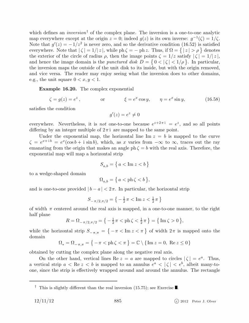
Example 16.20. The complex exponential

ζ = g(z) = ez , or ξ = ex cos y, η = ex sin y, (16.58)

satisfies the conditiong′(z) = ez 6= 0

everywhere. Nevertheless, it is not one-to-one because ez+2π i = ez, and so all pointsdiffering by an integer multiple of 2π i are mapped to the same point.

Under the exponential map, the horizontal line Im z = b is mapped to the curveζ = ex+ i b = ex(cos b+ i sin b), which, as x varies from −∞ to ∞, traces out the rayemanating from the origin that makes an angle ph ζ = b with the real axis. Therefore, theexponential map will map a horizontal strip

Sa,b =a < Im z < b

to a wedge-shaped domainΩa,b =

a < ph ζ < b

,

and is one-to-one provided | b− a | < 2π. In particular, the horizontal strip

S−π/2,π/2 =− 1

2 π < Im z < 12 π

of width π centered around the real axis is mapped, in a one-to-one manner, to the righthalf plane

R = Ω−π/2,π/2 =− 1

2π < ph ζ < 1

2π=Im ζ > 0

,

while the horizontal strip S−π,π =−π < Im z < π

of width 2π is mapped onto the

domainΩ∗ = Ω−π,π =

−π < ph ζ < π

= C \ Im z = 0, Re z ≤ 0

obtained by cutting the complex plane along the negative real axis.

On the other hand, vertical lines Re z = a are mapped to circles | ζ | = ea. Thus,a vertical strip a < Re z < b is mapped to an annulus ea < | ζ | < eb, albeit many-to-one, since the strip is effectively wrapped around and around the annulus. The rectangle

† This is slightly different than the real inversion (15.75); see Exercise .

12/11/12 885 c© 2012 Peter J. Olver

Figure 16.15. The mapping ζ = ez.

Figure 16.16. The Effect of ζ = z2 on Various Domains.

R =a < x < b,−π < y < π

of height 2π is mapped in a one-to-one fashion on an

annulus that has been cut along the negative real axis. See Figure 16.15.

Example 16.21. The squaring map

ζ = g(z) = z2, or ξ = x2 − y2, η = 2xy, (16.59)

is analytic on all of C, but is not one-to-one. Its inverse is the square root functionz =

√ζ , which, as we noted in Section 16.1, is doubly-valued, except at the origin z =

0. Furthermore, the derivative g′(z) = 2z vanishes at z = 0, violating the invertibilitycondition (16.52). However, once we restrict to a simply connected subdomain Ω thatdoes not contain 0, the function g(z) = z2 does define a one-to-one mapping, whoseinverse z = g−1(ζ) =

√ζ is a well-defined, analytic and single-valued branch of the square

root function.

The effect of the squaring map on a point z is to square its modulus, | ζ | = | z |2, whiledoubling its angle, ph ζ = ph z2 = 2 ph z. Thus, for example, the upper right quadrant

Q =x > 0, y > 0

=0 < ph z < 1

2 π

is mapped onto the upper half plane

U = g(Q) =η = Im ζ > 0

=0 < ph ζ < π

.

The inverse function maps a point ζ ∈ U back to its unique square root z =√ζ that lies

in the quadrant Q. Similarly, a quarter disk

Qρ =0 < | z | < ρ, 0 < ph z < 1

2 π

of radius ρ is mapped to a half disk

Uρ2 = g(Ω) =0 < | ζ | < ρ2, Im ζ > 0

of radius ρ2. On the other hand, the unit square S =0 < x < 1, 0 < y < 1

is mapped

to a curvilinear triangular domain, as indicated in Figure 16.16; the edges of the square

12/11/12 886 c© 2012 Peter J. Olver

on the real and imaginary axes map to the two halves of the straight base of the triangle,while the other two edges become its curved sides.

Example 16.22. A particularly important example is the analytic map

ζ =z − 1

z + 1=

x2 + y2 − 1

(x+ 1)2 + y2+ i

2y

(x+ 1)2 + y2, (16.60)

where we derived the formulae for its real and imaginary parts in (16.14). The map isone-to-one with analytic inverse

z =1 + ζ

1− ζ=

1− ξ2 − η2

(1− ξ)2 + η2+ i

2η

(1− ξ)2 + η2, (16.61)

provided z 6= −1 and ζ 6= 1. This particular analytic map has the important propertyof mapping the right half plane R =

x = Re z > 0

to the unit disk D =

| ζ |2 < 1

.

Indeed, by (16.61)

| ζ |2 = ξ2 + η2 < 1 if and only if x =1− ξ2 − η2

(1− ξ)2 + η2> 0.

Note that the denominator does not vanish on the interior of the disk.

The complex functions (16.56, 57, 60) are particular examples of linear fractional trans-formations

ζ =α z + β

γ z + δ, (16.62)

which form one of the most important classes of analytic maps. Here α, β, γ, δ are arbitrarycomplex constants, subject to the restriction

α δ − β γ 6= 0,

since otherwise (16.62) reduces to a trivial constant (and non-invertible) map. (Why?)

Example 16.23. The linear fractional transformation

ζ =z − α

α z − 1where |α | < 1, (16.63)

maps the unit disk to itself, moving the origin z = 0 to the point ζ = α. To prove this, wenote that

| z − α |2 = (z − α)(z − α) = | z |2 − αz − α z + |α |2,|αz − 1 |2 = (α z − 1)(αz − 1) = |α |2 | z |2 − α z − α z + 1.

Subtracting these two formulae,

| z − α |2 − |αz − 1 |2 =(1− |α |2

) (| z |2 − 1

)< 0, whenever | z | < 1, |α | < 1.

Thus, | z − α | < |αz − 1 |, which implies that

| ζ | = | z − α ||αz − 1 | < 1 provided | z | < 1, |α | < 1,

12/11/12 887 c© 2012 Peter J. Olver

f

θ

θ

Figure 16.17. A Conformal Map.

and hence ζ lies within the unit disk.

The rotations (16.55) also map the unit disk to itself, while preserving the origin. Itcan be proved, [4], that the only invertible analytic mappings that take the unit disk toitself are obtained by composing such a linear fractional transformation with a rotation.

Proposition 16.24. If ζ = g(z) is a one-to-one analytic map that takes the unit

disk to itself, then

g(z) = e iϕ z − α

α z − 1for some |α | < 1, 0 ≤ ϕ < 2π. (16.64)

Additional specific properties of linear fractional transformations are outlined in theexercises.

Conformality

A remarkable geometrical characterization of complex analytic functions is that, atnon-critical points, they preserve angles. The mathematical term for this property isconformal mapping . Conformality makes sense for any inner product space, although inpractice one usually deals with Euclidean space equipped with the standard dot product.

Definition 16.25. A function g:Rn → Rn is called conformal if it preserves angles.

But what does it mean to “preserve angles”? In the Euclidean norm, the angle betweentwo vectors is defined by their dot product, as in (3.20). However, most analytic maps arenonlinear, and so will not map vectors to vectors since they will typically map straightlines to curves. However, if we interpret “angle” to mean the angle between two curves,as illustrated in Figure 16.17, then we can make sense of the conformality requirement.Consequently, in order to realize complex functions as conformal maps, we first need tounderstand their effect on curves.

In general, a curve C ∈ C in the complex plane is parametrized by a complex-valuedfunction

z(t) = x(t) + i y(t), a < t < b, (16.65)

that depends on a real parameter t. Note that there is no essential difference between acomplex plane curve (16.65) and a real plane curve, as in (A.1); we have merely switched

from vector notation x(t) = ( x(t), y(t) )Tto complex notation z(t) = x(t)+ i y(t). All the

usual vectorial curve terminology (closed, simple, piecewise smooth, etc.), as summarized

12/11/12 888 c© 2012 Peter J. Olver

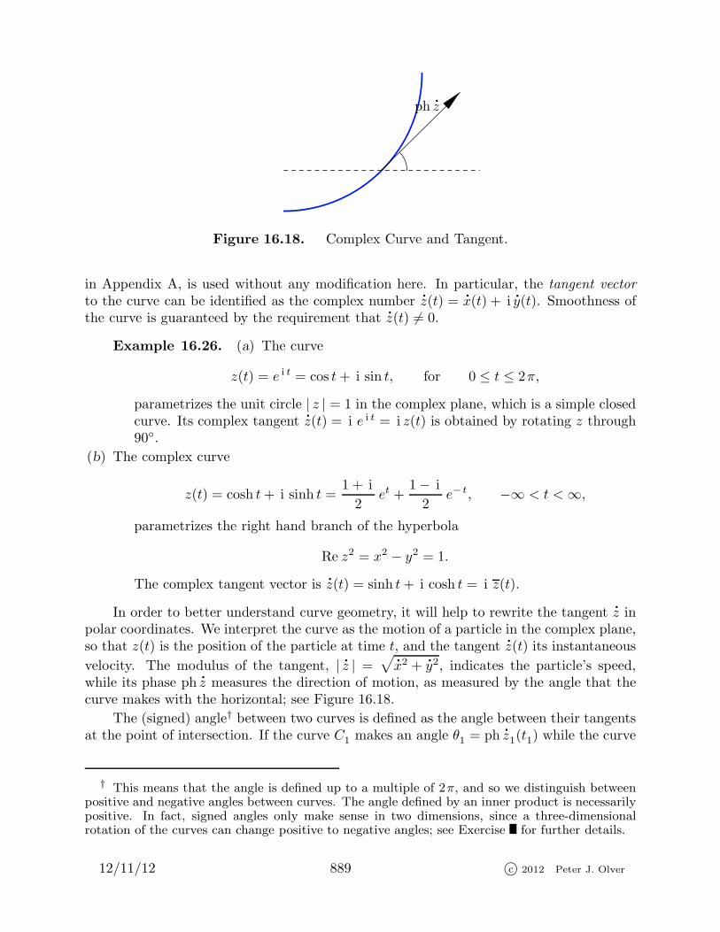
ph

z

Figure 16.18. Complex Curve and Tangent.

in Appendix A, is used without any modification here. In particular, the tangent vector

to the curve can be identified as the complex number

z(t) =

x(t) + i

y(t). Smoothness ofthe curve is guaranteed by the requirement that

z(t) 6= 0.

Example 16.26. (a) The curve

z(t) = e i t = cos t+ i sin t, for 0 ≤ t ≤ 2π,

parametrizes the unit circle | z | = 1 in the complex plane, which is a simple closedcurve. Its complex tangent

z(t) = i e i t = i z(t) is obtained by rotating z through90.

(b) The complex curve

z(t) = cosh t+ i sinh t =1 + i

2et +

1− i

2e−t, −∞ < t <∞,

parametrizes the right hand branch of the hyperbola

Re z2 = x2 − y2 = 1.

The complex tangent vector is

z(t) = sinh t+ i cosh t = i z(t).

In order to better understand curve geometry, it will help to rewrite the tangent

z inpolar coordinates. We interpret the curve as the motion of a particle in the complex plane,so that z(t) is the position of the particle at time t, and the tangent

z(t) its instantaneous

velocity. The modulus of the tangent, |

z | =√

x2 +

y2, indicates the particle’s speed,while its phase ph

z measures the direction of motion, as measured by the angle that thecurve makes with the horizontal; see Figure 16.18.

The (signed) angle† between two curves is defined as the angle between their tangentsat the point of intersection. If the curve C1 makes an angle θ1 = ph

z1(t1) while the curve

† This means that the angle is defined up to a multiple of 2π, and so we distinguish betweenpositive and negative angles between curves. The angle defined by an inner product is necessarilypositive. In fact, signed angles only make sense in two dimensions, since a three-dimensionalrotation of the curves can change positive to negative angles; see Exercise for further details.

12/11/12 889 c© 2012 Peter J. Olver

C2 has angle θ2 = ph

z2(t2) at the common point z = z1(t1) = z2(t2), then the angle θbetween C1 and C2 at z is their difference

θ = θ2 − θ1 = ph

z2 − ph

z1 = ph

(

z2

z1

). (16.66)

Now, suppose we are given an analytic map ζ = g(z). A curve C parametrized by z(t)will be mapped to a new curve Γ = g(C) parametrized by the composition ζ(t) = g(z(t)).The tangent to the image curve is related to that of the original curve by the chain rule:

dζ

dt=dg

dz

dz

dt, or

ζ(t) = g′(z(t))

z(t). (16.67)

Therefore, the effect of the analytic map on the tangent vector

z is to multiply it by thecomplex number g′(z). If the analytic map satisfies our key assumption g′(z) 6= 0, then

ζ 6= 0, and so the image curve is guaranteed to be smooth.

According to equation (16.67),

|

ζ | = | g′(z)

z | = | g′(z) | |

z |. (16.68)

Thus, the speed of motion along the new curve ζ(t) is multiplied by a factor ρ = | g′(z) | > 0.The magnification factor ρ depends only upon the point z and not how the curve passesthrough it. All curves passing through the point z are speeded up (or slowed down if ρ < 1)by the same factor! Similarly, the angle that the new curve makes with the horizontal isgiven by

ph

ζ = ph(g′(z)

z)= ph g′(z) + ph

z, (16.69)

since the phase of the product of two complex numbers is the sum of their individual phases,(3.82). Therefore, the tangent angle of the curve is increased by an amount φ = ph g′(z),which means that the tangent is been rotated through an angle φ. Again, the increase intangent angle only depends on the point z, and all curves passing through z are rotatedby the same amount φ. As a result, the angle between any two curves is preserved. Moreprecisely, if C1 is at angle θ1 and C2 at angle θ2 at a point of intersection, then their imagesΓ1 = g(C1) and Γ2 = g(C2) are at angles ψ1 = θ1+φ and ψ2 = θ2+φ. The angle betweenthe two image curves is the difference

ψ2 − ψ1 = (θ2 + φ) − (θ1 + φ) = θ2 − θ1,

which is the same as the angle between the original curves. This establishes the confor-mality or angle-preservation property of analytic maps.

Theorem 16.27. If ζ = g(z) is an analytic function and g′(z) 6= 0, then g defines a

conformal map.

Remark : The converse is also valid: Every planar conformal map comes from a com-plex analytic function with nonvanishing derivative. A proof is outlined in Exercise .

12/11/12 890 c© 2012 Peter J. Olver

Figure 16.19. Conformality of z2.

Figure 16.20. The Joukowski Map.

The conformality of analytic functions is all the more surprising when one revisitselementary examples. In Example 16.21, we discovered that the function w = z2 mapsa quarter plane to a half plane, and therefore doubles the angle between the coordinateaxes at the origin! Thus g(z) = z2 is most definitely not conformal at z = 0. Theexplanation is, of course, that z = 0 is a critical point, g′(0) = 0, and Theorem 16.27 onlyguarantees conformality when the derivative is nonzero. Amazingly, the map preservesangles everywhere else! Somehow, the angle at the origin is doubled, while angles at allnearby points are preserved. Figure 16.19 illustrates this remarkable and counter-intuitivefeat. The left hand figure shows the coordinate grid, while on the right are the images ofthe horizontal and vertical lines under the map z2. Note that, except at the origin, theimage curves continue to meet at 90 angles, in accordance with conformality.

Example 16.28. A particularly interesting conformal transformation is given by theJoukowski map

ζ =1

2

(z +

1

z

). (16.70)

12/11/12 891 c© 2012 Peter J. Olver

It is used in the study of flows around airplane wings, and named after the pioneeringRussian aero- and hydro-dynamics researcher Nikolai Zhukovskii (Joukowski). Since

dζ

dz=

1

2

(1− 1

z2

)= 0 if and only if z = ±1,

the Joukowski map is conformal except at the critical points z = ±1, as well as at thesingularity z = 0 where it is not defined.

If z = e i θ lies on the unit circle, then

ζ = 12

(e i θ + e− i θ

)= cos θ,

lies on the real axis, with −1 ≤ ζ ≤ 1. Thus, the Joukowski map squashes the unit circledown to the real line segment [−1, 1]. The images of points outside the unit circle fill therest of the ζ plane, as do the images of the (nonzero) points inside the unit circle. Indeed,if we solve (16.70) for

z = ζ ±√ζ2 − 1 , (16.71)

we see that every ζ except ±1 comes from two different points z; for ζ not on the criticalline segment [−1, 1], one point lies inside and and one lies outside the unit circle, whereasif −1 < ζ < 1, the points are situated directly above and below it on the circle. Therefore,(16.70) defines a one-to-one conformal map from the exterior of the unit circle

| z | > 1

onto the exterior of the unit line segment C \ [−1, 1].

Under the Joukowski map, the concentric circles | z | = r 6= 1 are mapped to ellipseswith foci at ±1 in the ζ plane; see Figure 16.20. The effect on circles not centered atthe origin is quite interesting. The image curves take on a wide variety of shapes; severalexamples are plotted in Figure 16.21. If the circle passes through the singular point z = 1,then its image is no longer smooth, but has a cusp at ζ = 1; this happens in the last 5of the figures. Some of the image curves have the shape of the cross-section through anairplane wing or airfoil . Later we will see how to construct the physical fluid flow aroundsuch an airfoil, which proved to be a critical step in early airplane design.

Composition and The Riemann Mapping Theorem

One of the strengths of the method of conformal mapping is that one can build up lotsof complicated examples by simply composing elementary mappings. The method restson the simple fact that the composition of two complex analytic functions is also complexanalytic. This is the complex counterpart of the result, learned in first year calculus, thatthe composition of two differentiable functions is itself differentiable.

Proposition 16.29. If w = f(z) is an analytic function of the complex variable

z = x+ i y, and ζ = g(w) is an analytic function of the complex variable w = u+ i v, thenthe composition† ζ = h(z) ≡ g f(z) = g(f(z)) is an analytic function of z.

† Of course, to properly define the composition, we need to ensure that the range of the functionw = f(z) is contained in the domain of the function ζ = g(w).

12/11/12 892 c© 2012 Peter J. Olver

Center: .1Radius: .5

Center: .2 + iRadius: 1

Center: 1 + iRadius: 1

Center: −2 + 3 iRadius: 3

√2 ≈ 4.2426

Center: .2 + iRadius: 1.2806

Center: .1 + .3 iRadius: .9487

Center: .1 + .1 iRadius: 3

√2 ≈ 4.2426

Center: −.2 + .1 iRadius: 1.2042

Figure 16.21. Airfoils Obtained from Circles via the Joukowski Map.

Proof : The proof that the composition of two differentiable functions is differentiableis identical to the real variable version, [9, 171], and need not be reproduced here. Thederivative of the composition is explicitly given by the usual chain rule:

d

dzg f(z) = g′(f(z)) f ′(z), or, in Leibnizian notation,

dζ

dz=dζ

dw

dw

dz. (16.72)

Further details are left to the reader. Q.E.D.

If both f and g are one-to-one, so is the composition h = g f . Moreover, the compo-sition of two conformal maps is also conformal, a fact that is immediate from the definition,or by using the chain rule (16.72) to show that

h′(z) = g′(f(z)) f ′(z) 6= 0 provided g′(f(z)) 6= 0 and f ′(z) 6= 0.

Thus, if f and g satisfy the conformality condition (16.52), so does h = g f . Q.E.D.

Example 16.30. As we learned in Example 16.20, the exponential function

w = ez

maps the horizontal strip S = −12 π < Im z < 1

2 π conformally onto the right half planeR = Re w > 0. On the other hand, Example 16.22 tells us that the linear fractionaltransformation

ζ =w − 1

w + 1

12/11/12 893 c© 2012 Peter J. Olver

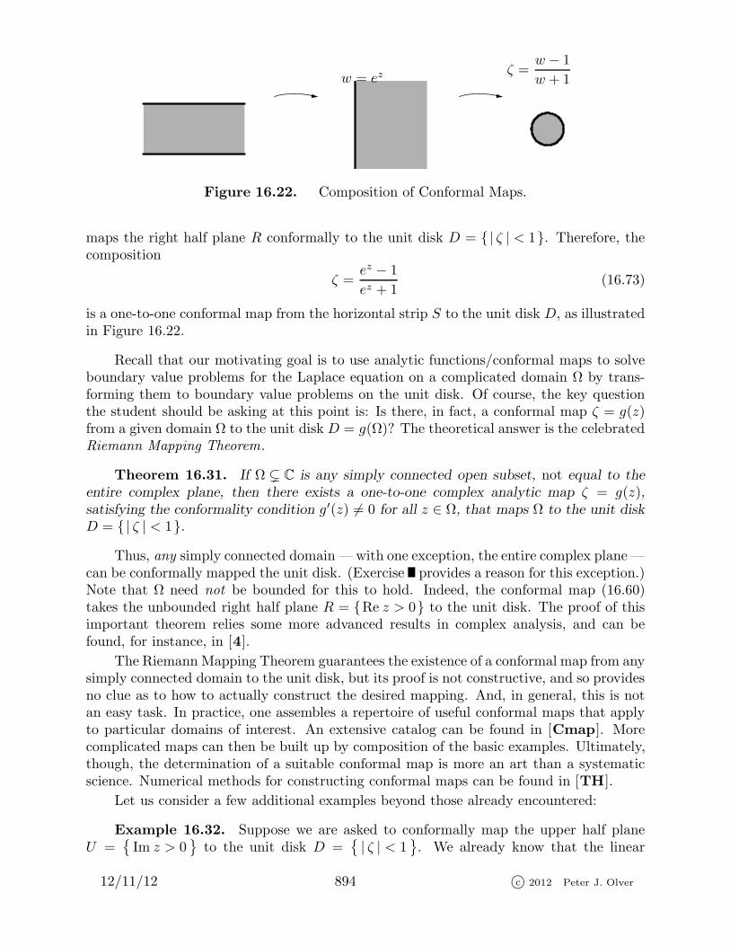
w = ezζ =

w − 1

w + 1

Figure 16.22. Composition of Conformal Maps.

maps the right half plane R conformally to the unit disk D = | ζ | < 1. Therefore, thecomposition

ζ =ez − 1

ez + 1(16.73)

is a one-to-one conformal map from the horizontal strip S to the unit disk D, as illustratedin Figure 16.22.

Recall that our motivating goal is to use analytic functions/conformal maps to solveboundary value problems for the Laplace equation on a complicated domain Ω by trans-forming them to boundary value problems on the unit disk. Of course, the key questionthe student should be asking at this point is: Is there, in fact, a conformal map ζ = g(z)from a given domain Ω to the unit disk D = g(Ω)? The theoretical answer is the celebratedRiemann Mapping Theorem.

Theorem 16.31. If Ω ( C is any simply connected open subset, not equal to the

entire complex plane, then there exists a one-to-one complex analytic map ζ = g(z),satisfying the conformality condition g′(z) 6= 0 for all z ∈ Ω, that maps Ω to the unit disk

D = | ζ | < 1.

Thus, any simply connected domain— with one exception, the entire complex plane—can be conformally mapped the unit disk. (Exercise provides a reason for this exception.)Note that Ω need not be bounded for this to hold. Indeed, the conformal map (16.60)takes the unbounded right half plane R = Re z > 0 to the unit disk. The proof of thisimportant theorem relies some more advanced results in complex analysis, and can befound, for instance, in [4].

The Riemann Mapping Theorem guarantees the existence of a conformal map from anysimply connected domain to the unit disk, but its proof is not constructive, and so providesno clue as to how to actually construct the desired mapping. And, in general, this is notan easy task. In practice, one assembles a repertoire of useful conformal maps that applyto particular domains of interest. An extensive catalog can be found in [Cmap]. Morecomplicated maps can then be built up by composition of the basic examples. Ultimately,though, the determination of a suitable conformal map is more an art than a systematicscience. Numerical methods for constructing conformal maps can be found in [TH].

Let us consider a few additional examples beyond those already encountered:

Example 16.32. Suppose we are asked to conformally map the upper half planeU =

Im z > 0

to the unit disk D =

| ζ | < 1

. We already know that the linear

12/11/12 894 c© 2012 Peter J. Olver

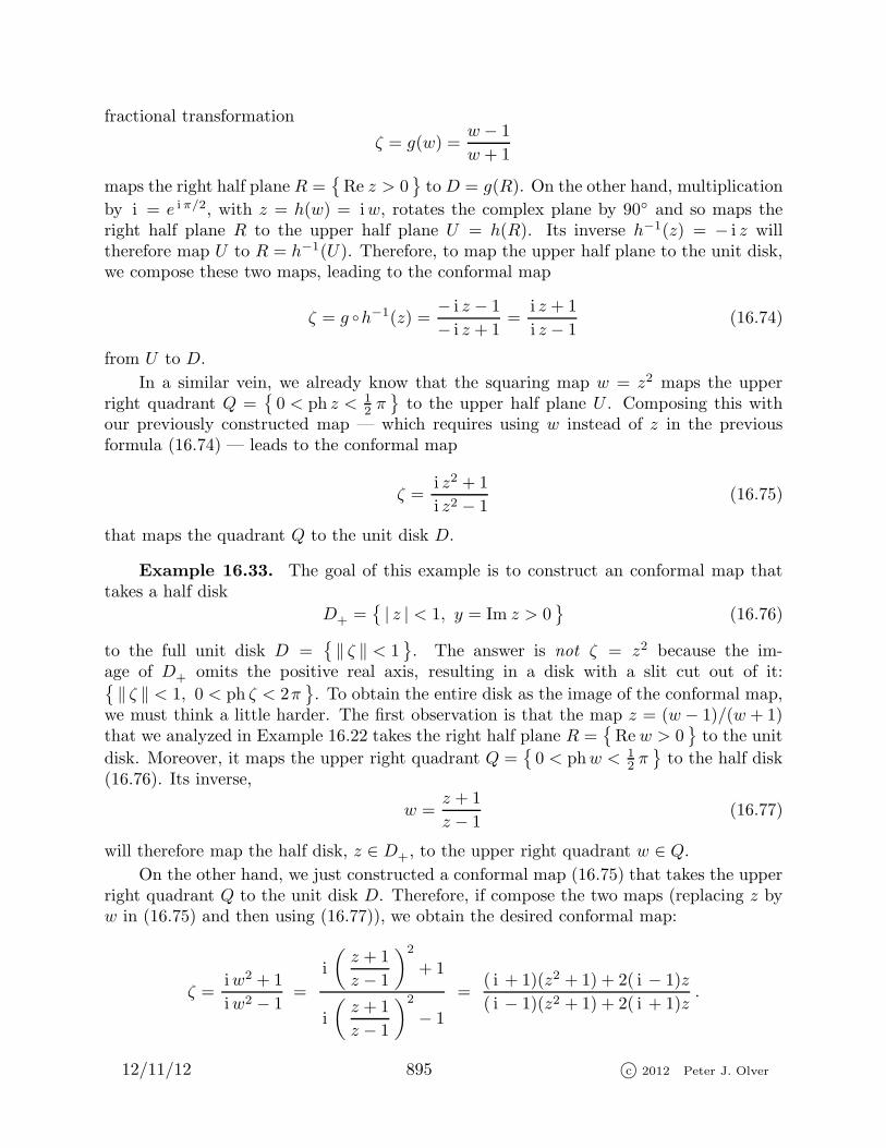
fractional transformation

ζ = g(w) =w − 1

w + 1

maps the right half plane R =Re z > 0

toD = g(R). On the other hand, multiplication

by i = e iπ/2, with z = h(w) = iw, rotates the complex plane by 90 and so maps theright half plane R to the upper half plane U = h(R). Its inverse h−1(z) = − i z willtherefore map U to R = h−1(U). Therefore, to map the upper half plane to the unit disk,we compose these two maps, leading to the conformal map

ζ = g h−1(z) =− i z − 1

− i z + 1=

i z + 1

i z − 1(16.74)

from U to D.

In a similar vein, we already know that the squaring map w = z2 maps the upperright quadrant Q =

0 < ph z < 1

2 πto the upper half plane U . Composing this with

our previously constructed map — which requires using w instead of z in the previousformula (16.74) — leads to the conformal map

ζ =i z2 + 1

i z2 − 1(16.75)

that maps the quadrant Q to the unit disk D.

Example 16.33. The goal of this example is to construct an conformal map thattakes a half disk

D+ =| z | < 1, y = Im z > 0

(16.76)

to the full unit disk D =‖ ζ ‖ < 1

. The answer is not ζ = z2 because the im-

age of D+ omits the positive real axis, resulting in a disk with a slit cut out of it:‖ ζ ‖ < 1, 0 < ph ζ < 2π

. To obtain the entire disk as the image of the conformal map,

we must think a little harder. The first observation is that the map z = (w − 1)/(w + 1)that we analyzed in Example 16.22 takes the right half plane R =

Re w > 0

to the unit

disk. Moreover, it maps the upper right quadrant Q =0 < phw < 1

2 πto the half disk

(16.76). Its inverse,

w =z + 1

z − 1(16.77)

will therefore map the half disk, z ∈ D+, to the upper right quadrant w ∈ Q.

On the other hand, we just constructed a conformal map (16.75) that takes the upperright quadrant Q to the unit disk D. Therefore, if compose the two maps (replacing z byw in (16.75) and then using (16.77)), we obtain the desired conformal map:

ζ =iw2 + 1

iw2 − 1=

i

(z + 1

z − 1

)2

+ 1

i

(z + 1

z − 1

)2

− 1

=( i + 1)(z2 + 1) + 2( i − 1)z

( i − 1)(z2 + 1) + 2( i + 1)z.

12/11/12 895 c© 2012 Peter J. Olver

The formula can be further simplified by multiplying numerator and denominator by i +1,and so

ζ = − iz2 + 2 i z + 1

z2 − 2 i z + 1.

The leading factor − i is unimportant and can be omitted, since it merely rotates the diskby −90, and so

ζ =z2 + 2 i z + 1

z2 − 2 i z + 1(16.78)

is an equally valid solution to our problem.

Finally, as noted in the preceding example, the conformal map guaranteed by theRiemann Mapping Theorem is not unique. Since the linear fractional transformations(16.63) map the unit disk to itself, we can compose them with any conformal Riemannmapping to produce additional conformal maps from a simply-connected domain to theunit disk. For example, composing (16.63) with (16.73) produces a family of mappings

ζ =1 + ez − α(1− ez)

α (1 + ez)− 1 + ez, (16.79)

which, for any |α | < 1, maps the strip S =− 1

2 π < Im z < 12 πonto the unit disk. With

a little more work, it can be shown that this is the only ambiguity, and so, for instance,(16.79) forms a complete list of one-to-ne conformal maps from S to D.

Annular Domains

The Riemann Mapping Theorem does not apply to non-simply connected domains.For purely topological reasons, a hole cannot be made to disappear under a one-to-onecontinuous mapping — much less a conformal map — and so a non-simply connecteddomain cannot be mapped in a on-to-one manner onto the unit disk. So we must lookelsewhere for a simple model domain.

The simplest non-simply connected domain is an annulus consisting of the pointsbetween two concentric circles

Ar,R =r < | ζ | < R

, (16.80)

which, for simplicity, is centered around the origin; see Figure 16.23. The case r = 0corresponds to a punctured disk, while R = ∞ gives the exterior of a disk or radius r. Itcan be proved, [Cmap], that any other domain with a single hole can be mapped to anannulus. The annular radii r, R are not uniquely specified; indeed the linear map ζ = αzmaps the annulus (16.80) to a rescaled annulus Aρr,ρR whose inner and outer radii have

both been scaled by the factor ρ = |α |. But the ratio† r/R of the inner to outer radius ofthe annulus is uniquely specified; annuli with different ratios cannot be mapped to eachother by a conformal map.

† If r = 0 or R = ∞, but not both, then r/R = 0 by convention. The punctured plane, wherer = 0 and R = ∞ remains a separate case.

12/11/12 896 c© 2012 Peter J. Olver

Figure 16.23. An Annulus.

Example 16.34. Let c > 0. Consider the domain

Ω =| z | < 1 and | z − c | > c

contained between two nonconcentric circles. To keep the computations simple, we takethe outer circle to have radius 1 (which can always be arranged by scaling, anyway) whilethe inner circle has center at the point z = c on the real axis and radius c, which meansthat it passes through the origin. We must restrict c < 1

2 in order that the inner circle notoverlap with the outer circle. Our goal is to conformally map this non-concentric annulardomain to a concentric annulus of the form

Ar,1 =r < | ζ | < 1

by a conformal map ζ = g(z).

Now, according, to Example 16.23, a linear fractional transformation of the form

ζ = g(z) =z − α

αz − 1with |α | < 1 (16.81)

maps the unit disk to itself. Moreover, as remarked earlier, and demonstrated in Exercise, linear fractional transformations always map circles to circles. Therefore, we seek a

particular value of α that maps the inner circle | z − c | = c to a circle of the form | ζ | = rcentered at the origin. We choose α real and try to map the points 0 and 2c on the innercircle to the points r and −r on the circle | ζ | = r. This requires

g(0) = α = r, g(2c) =2c− α

2cα− 1= −r. (16.82)

Substituting the first into the second leads to the quadratic equation

cα2 − α+ c = 0.

12/11/12 897 c© 2012 Peter J. Olver

Figure 16.24. Conformal Map for Non-concentric Annulus.

There are two real solutions:

α =1−

√1− 4c2

2cand α =

1 +√1− 4c2

2c. (16.83)

Since 0 < c < 12, the second solution has α > 1, and hence is inadmissible. Therefore, the

first solution yields the required conformal map

ζ =z − 1 +

√1− 4c2

(1−√1− 4c2 ) z − 2c

.

Note in particular that the radius r = α of the inner circle in Ar,1 is not the same as

the radius c of the inner circle in Ω. For example, taking c = 25, equation (16.83) implies

α = 12, and hence the linear fractional transformation ζ =

2z − 1

z − 2maps the annular domain

Ω =| z | < 1,

∣∣ z − 25

∣∣ > 25

to the concentric annulus A = A1/2,1 =

12 < | ζ | < 1

. In

Figure 16.24, we plot the non-concentric circles in Ω that are mapped to concentric circlesin the annulus A.

Applications to Harmonic Functions and Laplace’s Equation

Let us now apply our newly acquired expertise in conformal mapping to the study ofharmonic functions and boundary value problems for the Laplace equation. Our goal wasto change a boundary value problem on a domain Ω into a boundary value problem onthe unit disk D that we know how to solve. To this end, suppose we know a conformalmap ζ = g(z) that takes z ∈ Ω to ζ ∈ D. As we know, the real and imaginary parts ofan analytic function F (ζ) defined on D define harmonic functions. Moreover, accordingto Proposition 16.29, the composition f(z) = F (g(z)) defines an analytic function whosereal and imaginary parts are harmonic functions on Ω. Thus, the conformal mapping canbe regarded as a change of variables between their harmonic real and imaginary parts. Infact, this property does not even require the harmonic function to be the real part of ananalytic function, i.e., we are not required to assume the existence of a harmonic conjugate.

12/11/12 898 c© 2012 Peter J. Olver

Proposition 16.35. If U(ξ, η) is a harmonic function of ξ, η, and

ζ = ξ + i η = p(x, y) + i q(x, y) = g(z) (16.84)

is any analytic function, then the composition

u(x, y) = U(p(x, y), q(x, y)) (16.85)

is a harmonic function of x, y.

Proof : This is a straightforward application of the chain rule:

∂u

∂x=∂U

∂ξ

∂ξ

∂x+∂U

∂η

∂η

∂x,

∂u

∂y=∂U

∂ξ

∂ξ

∂y+∂U

∂η

∂η

∂y,

∂2u

∂x2=∂2U

∂ξ2

(∂ξ

∂x

)2

+ 2∂2U

∂ξ ∂η

∂ξ

∂x

∂η

∂x+∂2U

∂η2

(∂η

∂x

)2

+∂U

∂ξ

∂2ξ

∂x2+∂U

∂η

∂2η

∂x2,

∂2u

∂y2=∂2U

∂ξ2

(∂ξ

∂y

)2

+ 2∂2U

∂ξ ∂η

∂ξ

∂y

∂η

∂y+∂2U

∂η2

(∂η

∂y

)2

+∂U

∂ξ

∂2ξ

∂y2+∂U

∂η

∂2η

∂y2.

Using the Cauchy–Riemann equations

∂ξ

∂x= − ∂η

∂y,

∂ξ

∂y=∂η

∂x,

for the analytic function ζ = ξ + i η, we find, after some algebra,

∆u =∂2u

∂x2+∂2u

∂y2=

[(∂ξ

∂x

)2

+

(∂η

∂x

)2] [

∂2U

∂ξ2+∂2U

∂η2

]= | g′(z) |2 ∆U,

where | g′(z) |2 = ( ∂ξ/∂x )2+ ( ∂η/∂x )

2. We conclude that whenever U(ξ, η) is any har-

monic function, and so solves the Laplace equation ∆U = 0 (in the ξ, η variables), thenu(x, y) is a solution to the Laplace equation ∆u = 0 in the x, y variables, and is thus alsoharmonic. Q.E.D.

This observation has profound consequences for boundary value problems arising inphysical applications. Suppose we wish to solve the Dirichlet problem

∆u = 0 in Ω, u = h on ∂Ω, (16.86)

on a simply connected domain† Ω( C. Let ζ = g(z) = p(x, y) + i q(x, y) be a one-to-oneconformal mapping from the domain Ω to the unit disk D, whose existence is guaranteedby the Riemann Mapping Theorem 16.31. (Although its explicit construction may be muchmore problematic.) Then the change of variables formula (16.85) will map the harmonicfunction u(x, y) on Ω to a harmonic function U(ξ, η) on D. Moreover, the boundary values

† The Riemann Mapping Theorem 16.31 tells us to exclude the case Ω = C. Indeed, this caseis devoid of boundary conditions, and so the problem does not admit a unique solution.

12/11/12 899 c© 2012 Peter J. Olver

of U = H on the unit circle ∂D correspond to those of u = h on ∂Ω by the same changeof variables formula:

h(x, y) = H(p(x, y), q(x, y)), for (x, y) ∈ ∂Ω. (16.87)

We conclude that U(ξ, η) solves the Dirichlet problem

∆U = 0 in D, U = H on ∂D.

But we already know how to solve the Dirichlet problem on the unit disk by the Poissonintegral formula (15.48)! Then the solution to the original boundary value problem isgiven by the composition formula u(x, y) = U

(p(x, y), q(x, y)

). Thus, the solution to

the Dirichlet problem on a unit disk can be used to solve the Dirichlet problem on morecomplicated planar domains — provided we know the appropriate conformal map.

Example 16.36. According to Example 16.22, the analytic function

ξ + i η = ζ =z − 1

z + 1=

x2 + y2 − 1

(x+ 1)2 + y2+ i

2y

(x+ 1)2 + y2(16.88)

maps the right half plane R =x = Re z > 0

to the unit disk D =

| ζ | < 1

. Propo-

sition 16.35 implies that if U(ξ, η) is a harmonic function in the unit disk, then

u(x, y) = U

(x2 + y2 − 1

(x+ 1)2 + y2,

2y

(x+ 1)2 + y2

)(16.89)

is a harmonic function on the right half plane. (This can, of courtse, be checked directlyby a rather unpleasant chain rule computation.)

To solve the Dirichlet boundary value problem

∆u = 0, x > 0, u(0, y) = h(y), (16.90)

on the right half plane, we adopt the change of variables (16.88) and use the Poissonintegral formula to construct the solution to the transformed Dirichlet problem

∆U = 0, ξ2 + η2 < 1, U(cosϕ, sinϕ) = H(ϕ), (16.91)

on the unit disk. The relevant boundary conditions are found as follows. Using the explicitform

x+ i y = z =1 + ζ

1− ζ=

(1 + ζ)(1− ζ)

| 1− ζ |2 =1 + ζ − ζ − | ζ |2

| 1− ζ |2 =1− ξ2 − η2 + 2 i η

(ξ − 1)2 + η2

for the inverse map, we see that the boundary point ζ = ξ + i η = e iϕ on the unit circle∂D will correspond to the boundary point

i y =2 η

(ξ − 1)2 + η2=

2 i sinϕ

(cosϕ− 1)2 + sin2 ϕ= i cot

ϕ

2(16.92)

on the imaginary axis ∂R =Re z = 0

. Thus, the boundary data h(y) on ∂R corresponds

to the boundary dataH(ϕ) = h

(cot 1

2 ϕ)

12/11/12 900 c© 2012 Peter J. Olver

on the unit circle. The Poisson integral formula (15.48) can then be applied to solve(16.91), from which we are able to reconstruct the solution (16.89) to the boundary valueproblem (16.89) on the half plane.

Let’s look at an explicit example. If the boundary data on the imaginary axis isprovided by the step function

u(0, y) = h(y) ≡

1, y > 0,

0, y < 0,

then the corresponding boundary data on the unit disk is a (periodic) step function

H(ϕ) =

1, 0 < ϕ < π,

0, π < ϕ < 2π,

that has values +1 on the upper semicircle, −1 on the lower semicircle, and jump discon-tinuities at ζ = ±1. According to the Poisson formula (15.48), the solution to the latterboundary value problem is given by

U(ξ, η) =1

2π

∫ π

0

1− ρ2

1 + ρ2 − 2ρ cos(ϕ− φ)dφ

=1

π

[tan−1

(1 + ρ

1− ρcot

ϕ

2

)+ tan−1

(1 + ρ

1− ρtan

ϕ

2

)],

whereξ = ρ cosϕ,

η = ρ sinϕ.

Finally, we use (16.89) to construct the solution on the upper half plane, although weshall spare the reader the messy details of the final formula. The result is depicted inFigure zpm1h .

Remark : The solution to the preceding Dirichlet boundary value problem is not, infact, unique, owing to the unboundedness of the domain. The solution that we pick out byusing the conformal map to the unit disk is the one that remains bounded at ∞. There areother solutions, but they are unbounded as | z | → ∞ and would correspond to solutionson the unit disk that have some form of delta function singularity in their boundary dataat the point −1; see Exercise .

Example 16.37. A non-coaxial cable. The goal of this example is to determinethe electrostatic potential inside a non-coaxial cylindrical cable with prescribed constantpotential values on the two bounding cylinders, as illustrated in Figure 16.25. Assumefor definiteness that the larger cylinder has radius 1, and centered at the origin, whilethe smaller cylinder has radius 2

5 , and is centered at z = 25 . The resulting electrostatic

potential will be independent of the longitudinal coordinate, and so can be viewed as aplanar potential in the annular domain contained between two circles representing thecross-sections of our cylinders. The desired potential must satisfy the Dirichlet boundaryvalue problem

∆u = 0 when | z | < 1 and∣∣ z − 2

5

∣∣ > 25 ,

u = a, when | z | = 1, and u = b when∣∣ z − 2

5

∣∣ = 25 .

12/11/12 901 c© 2012 Peter J. Olver

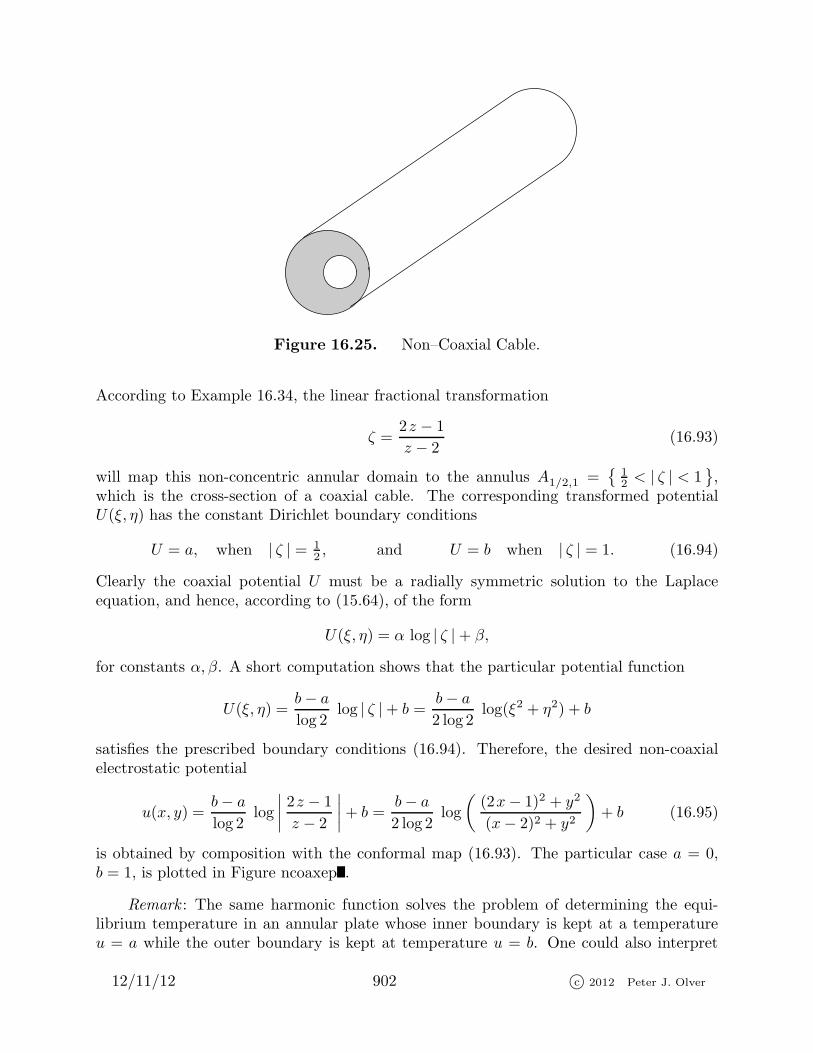
Figure 16.25. Non–Coaxial Cable.

According to Example 16.34, the linear fractional transformation

ζ =2z − 1

z − 2(16.93)

will map this non-concentric annular domain to the annulus A1/2,1 =

12 < | ζ | < 1

,

which is the cross-section of a coaxial cable. The corresponding transformed potentialU(ξ, η) has the constant Dirichlet boundary conditions

U = a, when | ζ | = 12, and U = b when | ζ | = 1. (16.94)

Clearly the coaxial potential U must be a radially symmetric solution to the Laplaceequation, and hence, according to (15.64), of the form

U(ξ, η) = α log | ζ |+ β,

for constants α, β. A short computation shows that the particular potential function

U(ξ, η) =b− a

log 2log | ζ |+ b =

b− a

2 log 2log(ξ2 + η2) + b

satisfies the prescribed boundary conditions (16.94). Therefore, the desired non-coaxialelectrostatic potential

u(x, y) =b− a

log 2log

∣∣∣∣2z − 1

z − 2

∣∣∣∣+ b =b− a

2 log 2log

((2x− 1)2 + y2

(x− 2)2 + y2

)+ b (16.95)

is obtained by composition with the conformal map (16.93). The particular case a = 0,b = 1, is plotted in Figure ncoaxep .

Remark : The same harmonic function solves the problem of determining the equi-librium temperature in an annular plate whose inner boundary is kept at a temperatureu = a while the outer boundary is kept at temperature u = b. One could also interpret

12/11/12 902 c© 2012 Peter J. Olver

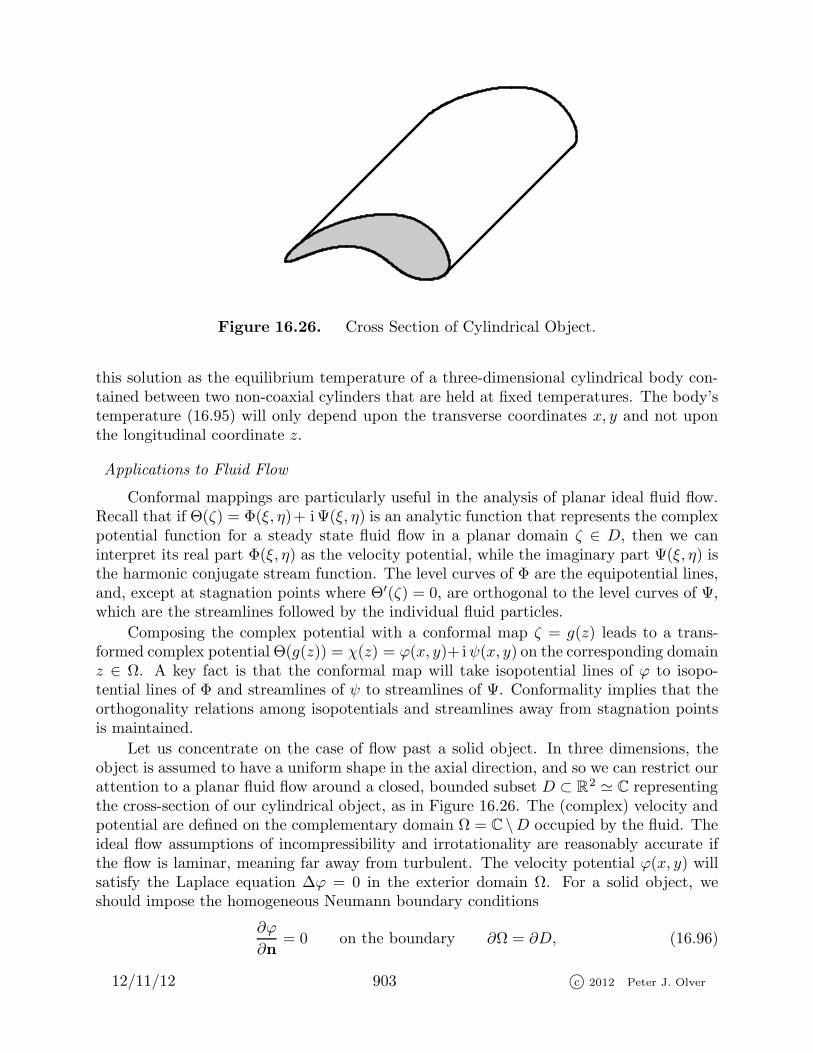
Figure 16.26. Cross Section of Cylindrical Object.

this solution as the equilibrium temperature of a three-dimensional cylindrical body con-tained between two non-coaxial cylinders that are held at fixed temperatures. The body’stemperature (16.95) will only depend upon the transverse coordinates x, y and not uponthe longitudinal coordinate z.

Applications to Fluid Flow

Conformal mappings are particularly useful in the analysis of planar ideal fluid flow.Recall that if Θ(ζ) = Φ(ξ, η)+ iΨ(ξ, η) is an analytic function that represents the complexpotential function for a steady state fluid flow in a planar domain ζ ∈ D, then we caninterpret its real part Φ(ξ, η) as the velocity potential, while the imaginary part Ψ(ξ, η) isthe harmonic conjugate stream function. The level curves of Φ are the equipotential lines,and, except at stagnation points where Θ′(ζ) = 0, are orthogonal to the level curves of Ψ,which are the streamlines followed by the individual fluid particles.

Composing the complex potential with a conformal map ζ = g(z) leads to a trans-formed complex potential Θ(g(z)) = χ(z) = ϕ(x, y)+ iψ(x, y) on the corresponding domainz ∈ Ω. A key fact is that the conformal map will take isopotential lines of ϕ to isopo-tential lines of Φ and streamlines of ψ to streamlines of Ψ. Conformality implies that theorthogonality relations among isopotentials and streamlines away from stagnation pointsis maintained.

Let us concentrate on the case of flow past a solid object. In three dimensions, theobject is assumed to have a uniform shape in the axial direction, and so we can restrict ourattention to a planar fluid flow around a closed, bounded subset D ⊂ R2 ≃ C representingthe cross-section of our cylindrical object, as in Figure 16.26. The (complex) velocity andpotential are defined on the complementary domain Ω = C \D occupied by the fluid. Theideal flow assumptions of incompressibility and irrotationality are reasonably accurate ifthe flow is laminar, meaning far away from turbulent. The velocity potential ϕ(x, y) willsatisfy the Laplace equation ∆ϕ = 0 in the exterior domain Ω. For a solid object, weshould impose the homogeneous Neumann boundary conditions

∂ϕ

∂n= 0 on the boundary ∂Ω = ∂D, (16.96)

12/11/12 903 c© 2012 Peter J. Olver

Figure 16.27. Flow Past a Solid Object.

indicating that there no fluid flux into the object. We note that, according to Exercise ,a conformal map will automatically preserve the Neumann boundary conditions.

In addition, since the flow is taking place on an unbounded domain, we need tospecify the fluid motion at large distances. We shall assume our object is placed in auniform horizontal flow, as in Figure 16.27. Thus, far away, the object will not affect theflow, and so the velocity should approximate the uniform velocity field v = ( 1, 0 )

T, where,

for simplicity, we choose our physical units so that the asymptotic speed of the fluid isequal to 1. Equivalently, the velocity potential should satisfy

ϕ(x, y) ≈ x, so ∇ϕ ≈(10

)when x2 + y2 ≫ 0.

Remark : An alternative physical interpretation is that the fluid is at rest, while theobject moves through the fluid at unit speed 1 in a horizontal direction. For example, thinkof an airplane flying through the air at constant speed. If we adopt a moving coordinatesystem by sitting inside the airplane, then the effect is as if the object is sitting still whilethe air is moving towards us at unit speed.

Example 16.38. The simplest example is a flat plate moving through the fluidin a horizontal direction. The plate’s cross-section is a horizontal line segment, and, forsimplicity, we take it to be the segment D = [−1, 1] lying on the real axis. If the plate isvery thin, it will have absolutely no effect on the horizontal flow of the fluid, and, indeed,the velocity potential is given by

ϕ(x, y) = x, for x+ i y ∈ Ω = C \ [−1, 1].

Note that ∇ϕ = ( 1, 0 )T, and hence this flow satisfies the Neumann boundary conditions

(16.96) on the horizontal segment D = ∂Ω. The corresponding complex potential is χ(z) =

12/11/12 904 c© 2012 Peter J. Olver

z, with complex velocity f(z) = χ′(z) = 1.

Example 16.39. Recall that the Joukowski conformal map defined by the analyticfunction

ζ = g(z) =1

2

(z +

1

z

)(16.97)

squashes the unit circle | z | = 1 down to the real line segment [−1, 1] in the ζ plane.Therefore, it will map the fluid flow outside the unit disk (which is the cross-section of acircular cylinder) to the fluid flow past the line segment, which, according to the previousexample, has complex potential Θ(ζ) = ζ. As a result, the complex potential for the flowpast a disk is the Joukowski function

χ(z) = Θ g(z) = g(z) =1

2

(z +

1

z

). (16.98)

Except for a factor of 12 , this agrees with the flow potential we derived in Example 16.17.

The difference is that, at large distances, the potential

χ(z) ≈ 12 z for | z | ≫ 1.

corresponds to uniform horizontal flow whose velocity(

12 , 0

)Tis half as fast. The discrep-

ancy between the two flows can easily be rectified by multiplying (16.98) by 2, whose onlyeffect is to speed up the flow.

Example 16.40. Let us next consider the case of a tilted plate in a uniformlyhorizontal fluid flow. Thus, the cross-section is the line segment

z(t) = t e i θ, −1 ≤ t ≤ 1,

obtained by rotating the horizontal line segment [−1, 1] through an angle θ, as in Fig-ure tilt . The goal is to construct a fluid flow past the tilted segment that is asymptoticallyhorizontal at large distance.

The critical observation is that, while the effect of rotating a plate in a fluid flow isnot so evident, rotating a circularly symmetric disk has no effect on in the flow aroundit. Thus, the rotation w = e− i θ z maps the Joukowski potential (16.98) to the complexpotential

Υ(w) = χ(e i θw) =1

2

(e i θw +

e− i θ

w

).

The streamlines of the induced flow are no longer asymptotically horizontal, but rather atan angle −θ. If we now apply the original Joukowski map (16.97) to the rotated flow, thecircle is again squashed down to the horizontal line segment, but the flow lines continueto be at angle −θ at large distances. Thus, if we then rotate the resulting flow throughan angle θ, the net effect will be to tilt the segment to the desired angle θ while rotatingthe streamlines to be asymptotically horizontal. Putting the pieces together, we have thefinal complex potential in the form

χ(z) = e i θ(z cos θ − i sin θ

√z2 − e−2 i θ

). (16.99)

Sample streamlines for the flow at several attack angles are plotted in Figure tilt .

12/11/12 905 c© 2012 Peter J. Olver

Example 16.41. As we discovered in Example 16.28, applying the Joukowski mapto off-center disks will, in favorable configurations, produce airfoil-shaped objects. Thefluid motion around such airfoils can thus be obtained by applying the Joukowski map tothe flow past such an off-center circle.

First, an affine mapw = α z + β

has the effect of moving the unit disk | z | ≤ 1 to the disk |w − β | ≤ |α | with centerβ and radius |α |. In particular, the boundary circle will continue to pass through thepoint w = 1 provided |α | = | 1− β |. Moreover, as noted in Example 16.18, the angularcomponent of α has the effect of a rotation, and so the streamlines around the new diskwill, asymptotically, be at an angle ϕ = phα with the horizontal. We then apply theJoukowski transformation

ζ =1

2

(w +

1

w

)=

1

2

(α z + β +

1

α z + β

)(16.100)

to map the disk to the airfoil shape. The resulting complex potential for the flow past theairfoil is obtained by substituting the inverse map

z =w − β

α=ζ − β +

√ζ2 − 1

α,

into the original potential (16.98), whereby

Θ(ζ) =1

2

(ζ − β +

√ζ2 − 1

α+α(ζ − β −

√ζ2 − 1

)

β2 + 1− 2β ζ

).

Since the streamlines have been rotated through an angle ϕ = phα, we then rotate thefinal result back by multiplying by e iϕ in order to see the effect of the airfoil tiled at anangle −ϕ in a horizontal flow. Sample streamlines are graphed in Figure airfoilnolift .

We can interpret all these examples as planar cross-sections of three-dimensional fluidflows past an airplane wing oriented in the longitudinal z direction. The wing is assumed tohave a uniform cross-section shape, and the flow not dependent upon the axial z coordinate.For sufficiently long wings flying in laminar (non-turbulent) flows, this model will be validaway from the wing tips. Underestanding the dynamics of more complicated airfoils withvarying cross-section and/or faster motion requires a fully three-dimensional fluid model.For such problems, complex analysis is no longer applicable, and, for the most part, onemust rely on large scale numerical integration. Only in recent years have computers becomesufficiently powerful to compute realistic three-dimensional fluid motions — and then onlyin reasonably “mild” scenarios†. The two-dimensional versions that have been analyzedhere still provide important clues to the behavior of a three-dimensional flow, as well asuseful initial approximations to the three-dimensional airplane wing design problem.

† The definition of mild relies on the magnitude of the Reynolds number, [13], an overallmeasure of the flow’s complexity.

12/11/12 906 c© 2012 Peter J. Olver

Unfortunately, there is a major flaw with the airfoils that we have just designed. Aswe will see, potential flows do not produce any lift, and hence such airplanes would notfly. Fortunately for us, the physical flow is not of this nature! In order to understand howlift enters into the picture, we need to study complex integration, and so we will return tothis example later. In Example 16.56, we shall construct an alternative flow past an airfoilthat continues to have the correct asymptotic behavior at large distances, while inducinga nonzero lift on the wing. This is the secret to flight.

Poisson’s Equation and the Green’s Function

Although designed for solving the homogeneous Laplace equation, the method of con-formal mapping can also be used to solve its inhomogeneous counterpart — the Poissonequation. As we learned in Chapter 15, to solve an inhomogeneous boundary value problemit suffices to solve the problem when the right hand side is a delta function concentratedat a point in the domain:

−∆u = δζ(x, y) = δ(x− ξ) δ(y− η), ζ = ξ + i η ∈ Ω,

sucject to homogeneous boundary conditions (Dirichlet or mixed) on ∂Ω. (As usual, weexclude pure Neumann boundary conditions due to lack of existence/uniqueness.) Thesolution

u(x, y) = Gζ(x, y) = G(x, y; ξ, η)

is the Green’s function for the given boundary value problem. With the Green’s functionin hand, the solution to the homogeneous boundary value problem under a general externalforcing,

−∆u = f(x, y),

is then provided by the superposition principle

u(x, y) =

∫ ∫

Ω

G(x, y; ξ, η) f(ξ, η) dξ dη. (16.101)

For the planar Poisson equation, the starting point is the logarithmic potential func-tion

u(x, y) = Re1

2πlog z =

1

2πlog | z | = 1

4πlog(x2 + y2), (16.102)

which solves the Dirichlet problem

−∆u = δ0(x, y), (x, y) ∈ D, u = 0 on ∂D,

on the unit disk D for an impulse concentrated at the origin; see Section 15.3 for details.How do we obtain the corresponding solution when the unit impulse is concentrated atanother point ζ = ξ + i η ∈ D instead of the origin? According to Example 16.23, thelinear fractional transformation

w = g(z) =z − ζ

ζ z − 1, where | ζ | < 1, (16.103)

12/11/12 907 c© 2012 Peter J. Olver

maps the unit disk to itself, moving the point z = ζ to the origin w = g(ζ) = 0. The

logarithmic potential U =1

2πlog |w | will thus be mapped to the Green’s function

G(x, y; ξ, η) =1

2πlog

∣∣∣∣∣z − ζ

ζ z − 1

∣∣∣∣∣ (16.104)

at the point ζ = ξ + i η. Indeed, by the properties of conformal mapping, since U isharmonic except at the singularity w = 0, the function (16.104) will also be harmonicexcept at the image point z = ζ. The fact that the mapping does not affect the deltafunction singularity is not hard to check; the details are relegated to Exercise . Moreover,since the conformal map does not alter the boundary | z | = 1, the function (16.104)continues to satisfy the homogeneous Dirichlet boundary conditions.

Formula (16.104) reproduces the Poisson formula (15.78) for the Green’s functionthat we previously derived by the method of images. This identification can be verifiedby substituting z = r e i θ, ζ = ρ e iϕ, or, more simply, by noting that the numerator inthe logarithmic fraction gives the potential due to a unit impulse at z = ζ, while thedenominator represents the image potential at z = 1/ ζ required to cancel out the effect ofthe interior potential on the boundary of the unit disk.

Now that we know the Green’s function on the unit disk, we can use the methodsof conformal mapping to produce the Green’s function for any other simply connecteddomain Ω( C.

Proposition 16.42. Let w = g(z) denote the conformal map that takes the domain

z ∈ Ω to the unit disk w ∈ D, guaranteed by the Riemann Mapping Theorem 16.31. Then

the Green’s function associated with homogeneous Dirichlet boundary conditions on Ω is

explicitly given by

G(z; ζ) =1

2πlog

∣∣∣∣∣g(z)− g(ζ)

g(ζ) g(z)− 1

∣∣∣∣∣ . (16.105)

Example 16.43. According to Example 16.22, the analytic function

w =z − 1

z + 1

maps the right half plane x = Re z > 0 to the unit disk | ζ | < 1. Therefore, by (16.105),the Green’s function for the right half plane has the form

G(z; ζ) =1

2πlog

∣∣∣∣∣∣∣∣∣

z − 1

z + 1− ζ − 1

ζ + 1

z − 1

z + 1

ζ − 1

ζ + 1− 1

∣∣∣∣∣∣∣∣∣

=1

2πlog

∣∣∣∣(ζ + 1)(z − ζ)

(z + 1)(z − ζ)

∣∣∣∣ . (16.106)

One can then write the solution to the Poisson equation in a superposition as in (16.101).

12/11/12 908 c© 2012 Peter J. Olver

16.5. Complex Integration.

The magic and power of calculus ultimately rests on the amazing fact that differen-tiation and integration are mutually inverse operations. And, just as complex functionshave many remarkable differentiability properties not enjoyed by their real siblings, so thesublime beauty and innate structure complex integration goes far beyond its more mun-dane real counterpart. In the remaining two sections of this chapter, we shall develop thebasics of complex integration theory and present a few of its important applications.

The first step is to motivate the definition of a complex integral. As you know, the

(definite) integral of a real function,

∫ b

a

f(t) dt, is evaluated on an interval [a, b ] ⊂ R.

In complex function theory, integrals are taken along curves in the complex plane, andthus have the flavor of the line integrals appearing in real vector calculus. Indeed, theidentification of a complex number z = x+ i y with a planar vector x = ( x, y )

Twill serve

to connect the two theories.

Consider a curve C in the complex plane, parametrized, as in (16.65), by z(t) =x(t) + i y(t) for a ≤ t ≤ b. We define the integral of the complex function f(z) along thecurve C to be the complex number

∫

C

f(z) dz =

∫ b

a

f(z(t))dz

dtdt. (16.107)

We shall always assume that the integrand f(z) is a well-defined complex function at eachpoint on the curve. Let us write out the integrand

f(z) = u(x, y) + i v(x, y)

in terms of its real and imaginary parts. Also,

dz =dz

dtdt =

(dx

dt+ i

dy

dt

)dt = dx+ i dy.

As a result, the complex integral (16.107) splits up into a pair of real line integrals:∫

C

f(z) dz =

∫

C

(u+ i v)(dx+ i dy) =

∫

C

(u dx− v dy) + i

∫

C

(v dx+ u dy). (16.108)

Example 16.44. Let us compute complex integrals∫

C

zn dz, (16.109)

of the monomial function f(z) = zn, where n is an integer, along several different curves.We begin with a straight line segment along the real axis connecting the points −1 to 1,which we parametrize by z(t) = t for −1 ≤ t ≤ 1. The defining formula (16.107) impliesthat the complex integral (16.109) reduces to a real integral:

∫

C

zn dz =

∫ 1

−1

tn dt =

0, n = 2k + 1 > 0 is odd ,2

n+ 1, n = 2k ≥ 0 is even.

12/11/12 909 c© 2012 Peter J. Olver

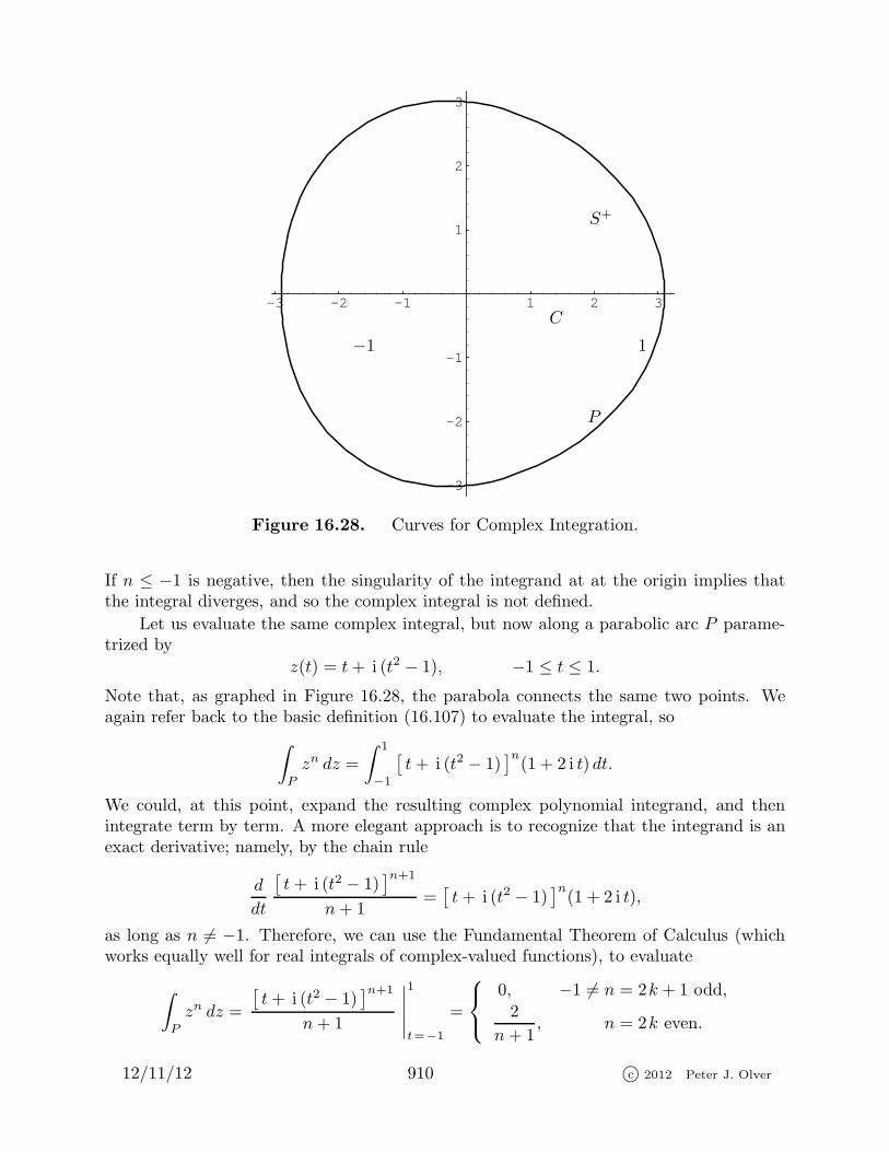
-3 -2 -1 1 2 3

-3

-2

-1

1

2

3

1−1

P

C

S+

Figure 16.28. Curves for Complex Integration.

If n ≤ −1 is negative, then the singularity of the integrand at at the origin implies thatthe integral diverges, and so the complex integral is not defined.

Let us evaluate the same complex integral, but now along a parabolic arc P parame-trized by

z(t) = t+ i (t2 − 1), −1 ≤ t ≤ 1.

Note that, as graphed in Figure 16.28, the parabola connects the same two points. Weagain refer back to the basic definition (16.107) to evaluate the integral, so

∫

P

zn dz =

∫ 1

−1

[t+ i (t2 − 1)

]n(1 + 2 i t) dt.

We could, at this point, expand the resulting complex polynomial integrand, and thenintegrate term by term. A more elegant approach is to recognize that the integrand is anexact derivative; namely, by the chain rule

d

dt

[t+ i (t2 − 1)

]n+1

n+ 1=[t+ i (t2 − 1)

]n(1 + 2 i t),

as long as n 6= −1. Therefore, we can use the Fundamental Theorem of Calculus (whichworks equally well for real integrals of complex-valued functions), to evaluate

∫

P

zn dz =

[t+ i (t2 − 1)

]n+1

n+ 1

∣∣∣∣∣

1

t=−1

=

0, −1 6= n = 2k + 1 odd,2

n+ 1, n = 2k even.

12/11/12 910 c© 2012 Peter J. Olver

Thus, when n ≥ 0 is a positive integer, we obtain the same result as before. Interestingly,in this case the complex integral is well-defined even when n is a negative integer because,unlike the real line segment, the parabolic path does not go through the singularity of zn

at z = 0. The case n = −1 needs to be done slightly differently, and integration of 1/zalong the parabolic path is left as an exercise for the reader — one that requires somecare. We recommend trying the exercise now, and then verifying your answer once wehave become a little more familiar with basic complex integration techniques.

Finally, let us try integrating around a semi-circular arc, again with the same endpoints−1 and 1. If we parametrize the semi-circle S+ by z(t) = e i t, 0 ≤ t ≤ π, we find

∫

S+

zn dz =

∫ π

0

zndz

dtdt =

∫ π

0

e int i e i t dt =

∫ π

0

i e i (n+1)t dt

=e i (n+1)t

n+ 1

∣∣∣∣π

t=0

=1− e i (n+1)π

n+ 1=

0, −1 6= n = 2k + 1 odd,

− 2

n+ 1, n = 2k even.

This value is the negative of the previous cases — but this can be explained by the factthat the circular arc is oriented to go from 1 to −1 whereas the line segment and parabolaboth go from −1 to 1. Just as with line integrals, the direction of the curve determines thesign of the complex integral; if we reverse direction, replacing t by −t, we end up with thesame value as the preceding two complex integrals. Moreover — again provided n 6= −1— it does not matter whether we use the upper semicircle or lower semicircle to go from−1 to 1 — the result is exactly the same. However, the case n = −1 is an exception tothis “rule”. Integrating along the upper semicircle S+ from 1 to −1 yields

∫

S+

dz

z=

∫ π

0

i dt = π i , (16.110)

whereas integrating along the lower semicircle S− from 1 to −1 yields the negative∫

S−

dz

z=

∫ −π

0

i dt = −π i . (16.111)

Hence, when integrating the function 1/z, it makes a difference which direction we goaround the origin.

Integrating zn for any integer n 6= −1 around an entire circle gives zero — irrespectiveof the radius. This can be seen as follows. We parametrize a circle of radius r by z(t) = re i t

for 0 ≤ t ≤ 2π. Then, by the same computation,

∮

C

zn dz =

∫ 2π

0

(rne int)(r i e i t) dt =

∫ 2π

0

i rn+1e i (n+1)t dt =rn+1

n+ 1e i (n+1)t

∣∣∣∣2π

t=0

= 0,

(16.112)provided n 6= −1. Here, as in Appendix A, the circle on the integral sign serves to remindus that we are integrating around a closed curve. The case n = −1 remains special.Integrating once around the circle in the counter-clockwise direction yields a nonzero result

∮

C

dz

z=

∫ 2π

0

i dt = 2π i . (16.113)

12/11/12 911 c© 2012 Peter J. Olver

Let us note that a complex integral does not depend on the particular parametrizationof the curve C. It does, however, depend upon the orientation of the curve: if we traversethe curve in the reverse direction, then the complex integral changes its sign:

∫

−C

f(z) dz = −∫

C

f(z) dz. (16.114)

Moreover, if we chop up the curve into two non-overlapping pieces, C = C1 ∪ C2, with acommon orientation, then the complex integral can be decomposed into a sum over thepieces: ∫

C1∪C2

f(z) =

∫

C1

f(z) dz +

∫

C2

f(z) dz. (16.115)

For instance, the integral (16.113) of 1/z around the circle is the difference of the individualsemicircular integrals (16.110–111); the lower semicircular integral acquires a negative signto flip its orientation so as to agree with that of the entire circle. All these facts areimmediate consequences of the basic properties of line integrals, or can be easily proveddirectly from the defining formula (16.107).

Note: In complex integration theory, a simple closed curve is often referred to as acontour , and so complex integration is sometimes referred to as contour integration. Unlessexplicitly stated, we always go around contours in the counter-clockwise direction.

Further experiments lead us to suspect that complex integrals are usually path-independent, and hence evaluate to zero around closed contours. One must be careful,though, as the integral (16.113) makes clear. Path independence, in fact, follows from thecomplex version of the Fundamental Theorem of Calculus.

Theorem 16.45. Let f(z) = F ′(z) be the derivative of a single-valued complex

function F (z) defined on a domain Ω ⊂ C. Let C ⊂ Ω be any curve with initial point αand final point β. Then

∫

C

f(z) dz =

∫

C

F ′(z) dz = F (β)− F (α). (16.116)

Proof : This follows immediately from the definition (16.107) and the chain rule:

∫

C

F ′(z) dz =

∫ b

a

F ′(z(t))dz

dtdt =

∫ b

a

d

dtF (z(t)) dt = F (z(b))− F (z(a)) = F (β)− F (α),

where α = z(a) and β = z(b) are the endpoints of the curve. Q.E.D.

For example, when n 6= −1, the function f(z) = zn is the derivative of the single-

valued function F (z) =1

n+ 1zn+1. Hence

∫

C

zn dz =βn+1

n+ 1− αn+1

n+ 1

12/11/12 912 c© 2012 Peter J. Olver

whenever C is a curve connecting α to β. When n < 0, the curve is not allowed to passthrough the origin, z = 0, as it is a singularity for zn.

In contrast, the function f(z) = 1/z is the derivative of the complex logarithm

log z = log | z |+ i ph z,

which is not single-valued on all of C \ 0, and so Theorem 16.45 cannot be applieddirectly. However, if our curve is contained within a simply connected subdomain thatdoes not include the origin, 0 6∈ Ω ⊂ C, then we can use any single-valued branch of thecomplex logarithm to evaluate the integral

∫

C

dz

z= log β − logα,

where α, β are the endpoints of the curve. Since the common multiples of 2π i cancel, theanswer does not depend upon which particular branch of the complex logarithm is chosenas long as we are consistent in our choice. For example, on the upper semicircle S+ ofradius 1 going from 1 to −1,

∫

S+

dz

z= log(−1)− log 1 = π i ,

where we use the branch of log z = log | z |+ i ph z with 0 ≤ ph z ≤ π. On the other hand,if we integrate on the lower semi-circle S− going from 1 to −1, we need to adopt a differentbranch, say that with −π ≤ ph z ≤ 0. With this choice, the integral becomes

∫

S−

dz

z= log(−1)− log 1 = −π i ,

thus reproducing (16.110, 111). Pay particular attention to the different values of log(−1)in the two cases!

The most important consequence of Theorem 16.45 is that, as long as the integrandf(z) has a single-valued anti-derivative, its complex integral is independent of the pathconnecting two points — the value only depends on the endpoints of the curve and nothow one gets from point α to point β.

Theorem 16.46. Let f(z) = F ′(z), where F (z) is a single-valued complex function

for z ∈ Ω. If C ⊂ Ω is any closed curve, then

∮

C

f(z) dz = 0. (16.117)

Conversely, if (16.117) holds for all closed curves C ⊂ Ω contained in the domain of

definition of f(z), then f admits a single-valued complex anti-derivative with F ′(z) = f(z).

Proof : We have already demonstrated the first statement. As for the second, wedefine

F (z) =

∫ z

z0

f(z) dz,

12/11/12 913 c© 2012 Peter J. Olver

Figure 16.29. Orientation of Domain Boundary.

where z0 ∈ Ω is any fixed point, and we choose any convenient curve C ⊂ Ω connecting†

z0 to z. (16.117) assures us that the value does not depend on the chosen path. The proofthat this formula does define an anti-derivative of f is left as an exercise, which can besolved in the same fashion as the case of a real line integral, cf. (22.42). Q.E.D.

The preceding considerations suggest the following fundamental theorem, due in itsgeneral form to Cauchy. Before stating it, we introduce the convention that a complexfunction f(z) is to be called analytic on a domain Ω ⊂ C provided it is analytic at everypoint inside Ω and, in addition, remains (at least) continuous on the boundary ∂Ω. WhenΩ is bounded, its boundary ∂Ω consists of one or more simple closed curves. In general,as in Green’s Theorem A.26, we orient ∂Ω so that the domain is always on our left handside. This means that the outermost boundary curve is traversed in the counter-clockwisedirection, but any interior holes are take on a clockwise orientation. Our convention isdepicted in Figure 16.29.

Theorem 16.47. If f(z) is analytic on a bounded domain Ω ⊂ C, then

∮

∂Ω

f(z) dz = 0. (16.118)

Proof : If we apply Green’s Theorem to the two real line integrals in (16.108), we find

∮

∂Ω

u dx− v dy =

∫ ∫

Ω

(− ∂v

∂x− ∂u

∂y

)= 0,

∮

∂Ω

v dx+ u dy =

∫ ∫

Ω

(∂u

∂x− ∂v

∂y

)= 0,

both of which vanish by virtue of the Cauchy–Riemann equations (16.22). Q.E.D.

If the domain of definition of our complex function f(z) is simply connected, then, bydefinition, the interior of any closed curve C ⊂ Ω is contained in Ω, and hence Cauchy’sTheorem 16.47 implies path independence of the complex integral within Ω.

† This assumes Ω is a connected domain; otherwise, apply the result to its individual connectedcomponents.

12/11/12 914 c© 2012 Peter J. Olver

CS

Ω

C

SK

Figure 16.30. Integration Around Two Closed Curves.

Corollary 16.48. If f(z) is analytic on a simply connected domain Ω ⊂ C, then its

complex integral

∫

C

f(z) dz for C ⊂ Ω is independent of path. In particular,

∮

C

f(z) dz = 0 (16.119)

for any closed curve C ⊂ Ω.

Remark : Simple connectivity of the domain is an essential hypothesis — our evalua-tion (16.113) of the integral of 1/z around thye unit circle provides a simple counterexampleto (16.119) in the non-simply connected domain Ω = C\0. Interestingly, this result alsoadmits a converse: a continuous function f(z) that satisfies (16.119) for all closed curvesis necessarily analytic; see [4] for a proof.

We will also require a slight generalization of this result.

Proposition 16.49. If f(z) is analytic in a domain that contains two simple closed

curves S and C, and the entire region lying between them, then, assuming they are oriented

in the same direction, ∮

C

f(z) dz =

∮

S

f(z) dz. (16.120)

Proof : If C and S do not cross each other, we let Ω denote the domain containedbetween them, so that ∂Ω = C ∪ S; see the first plot in Figure 16.30. According to

Cauchy’s Theorem 16.47,

∮

∂Ω

f(z) = 0. Now, our orientation convention for ∂Ω means

that the outer curve, say C, is traversed in the counter-clockwise direction, while the innercurve S has the opposite, clockwise orientation. Therefore, if we assign both curves thesame counter-clockwise orientation,

0 =

∮

∂Ω

f(z) =

∮

C

f(z) dz −∮

S

f(z) dz,

12/11/12 915 c© 2012 Peter J. Olver

proving (16.120).

If the two curves cross, we can construct a nearby curve K ⊂ Ω that neither crosses,as in the second sketch in Figure 16.30. By the preceding paragraph, each integral is equalto to that over the third curve,

∮

C

f(z) dz =

∮

K

f(z) dz =

∮

S

f(z) dz,

and formula (16.120) remains valid. Q.E.D.

Example 16.50. Consider the function f(z) = zn where n is an integer†. In(16.112), we already computed

∮

C

zn dz =

0, n 6= −1,

2π i , n = −1,(16.121)

when C is a circle centered at z = 0. When n ≥ 0, Theorem 16.45 immediately impliesthat the integral of zn is 0 over any closed curve in the plane. The same applies in thecases n ≤ −2 provided the curve does not pass through the singular point z = 0. Inparticular, the integral is zero around closed curves encircling the origin, even though zn

for n ≤ −2 has a singularity inside the curve and so Cauchy’s Theorem 16.47 does notapply as stated.

The case n = −1 has particular significance. Here, Proposition 16.49 implies thatthe integral is the same as the integral around a circle — provided the curve C also goesonce around the origin in a counter-clockwise direction. Thus (16.113) holds for any closedcurve that goes counter-clockwise once around the origin. More generally, if the curve goesseveral times around the origin‡, then

∮

C

dz

z= 2kπ i (16.122)

is an integer multiple of 2π i . The integer k is called the winding number of the curve C,and measures the total number of times C goes around the origin. For instance, if C windsthree times around 0 in a counter-clockwise fashion, then k = 3, while k = −5 indicatesthat the curve winds 5 times around 0 in a clockwise direction, as in Figure 16.31. Inparticular, a winding number k = 0 indicates that C is not wrapped around the origin. IfC represents a loop of string wrapped around a pole (the pole of 1/z at 0) then a windingnumber k = 0 would indicate that the string can be disentangled from the pole withoutcutting; nonzero winding numbers would indicate that the string is truly entangled§.

† When n is fractional or irrational, the integrals are not well-defined owing to the branchpoint at the origin.

‡ Such a curve is undoubtedly not simple and must necessarily cross over itself.

§ Actually, there are more subtle three-dimensional considerations that come into play, andeven strings with zero winding number cannot be removed from the pole without cutting if theyare linked in some nontrivial manner, cf. [115]. Can you think of an example?

12/11/12 916 c© 2012 Peter J. Olver

k = 0 k = 3 k = −5

Figure 16.31. Winding Numbers.

Lemma 16.51. If C is any simple closed curve, and a is any point not lying on C,then ∮

C

dz

z − a=

2π i , a inside C

0 a outside C.(16.123)

If a ∈ C, then the integral does not converge.

Proof : Note that the integrand f(z) = 1/(z − a) is analytic everywhere except atz = a, where it has a simple pole. If a is outside C, then Cauchy’s Theorem 16.47 applies,and the integral is zero. On the other hand, if a is inside C, then Proposition 16.49implies that the integral is equal to the integral around a circle centered at z = a. Thelatter integral can be computed directly by using the parametrization z(t) = a+ r e i t for0 ≤ t ≤ 2π, as in (16.113). Q.E.D.

Example 16.52. Let D ⊂ C be a closed and connected domain. Let a, b ∈ D betwo points in D. Then

∮

C

(1

z − a− 1

z − b

)dz =

∮

C

dz

z − a−∮

C

dz

z − b= 0

for any closed curve C ⊂ Ω = C \ D lying outside the domain D. This is because, byconnectivity of D, either C contains both points in its interior, in which case both integralsequal 2π i , or C contains neither point, in which case both integrals are 0. According toTheorem 16.46, the integrand admits a single-valued anti-derivative on the domain Ω, eventhough each individual term is the derivative of a multiply-valued complex logarithm. Theconclusion is that, while the individual logarithms are multiply-valued, their difference

F (z) = log(z − a)− log(z − b) (16.124)

is a consistent, single-valued complex function on all of Ω = C\D. The difference (16.124),in fact, an infinite number of possible values, differing by integer multiples of 2π i ; theambiguity can be removed by choosing one of its value at a single point in Ω. Theseconclusions rest on the fact that D is connected, and are not valid, say, for the twice-punctured plane C \ a, b.

We are sometimes interested in estimating the size of a complex integral. The basicinequality bounds it in terms of an arc length integral.

12/11/12 917 c© 2012 Peter J. Olver

Proposition 16.53. The modulus of the integral of the complex function f along a

curve C is bounded by the integral of its modulus with respect to arc length:

∣∣∣∣∫

C

f(z) dz

∣∣∣∣ ≤∫

C

| f(z) | ds. (16.125)

Proof : We begin with a simple lemma on real integrals of complex functions.

Lemma 16.54. Let f(t) be a complex-valued function depending on the real variable

a ≤ t ≤ b. Then ∣∣∣∣∣

∫ b

a

f(t)dt

∣∣∣∣∣ ≤∫ b

a

| f(t) | dt. (16.126)

Proof : If

∫ b

a

f(t) dt = 0, the inequality is trivial. Otherwise, let θ = ph

∫ b

a

f(t)dt.

Then, using Exercise 3.6.9,∣∣∣∣∣

∫ b

a

f(t) dt

∣∣∣∣∣ = Re

[e− i θ

∫ b

a

f(t) dt

]=

∫ b

a

Re[e− i θ f(t)

]dt ≤

∫ b

a

| f(t) | dt,

which proves the lemma. Q.E.D.

To prove the proposition, we write out the complex integral, and use (16.126) asfollows:

∣∣∣∣∫

C

f(z) dz

∣∣∣∣ =∣∣∣∣∣

∫ b

a

f(z(t))dz

dtdt

∣∣∣∣∣ ≤∫ b

a

| f(z(t)) |∣∣∣∣dz

dt

∣∣∣∣ dt =∫

C

| f(z) | ds,

since | dz | = |

z | dt =√

x2 +

y2 dt = ds is the arc length integral element (A.30). Q.E.D.

Corollary 16.55. If the curve C has length L = L(C), and f(z) is an analytic

function such that | f(z) | ≤M for all points z ∈ C, then

∣∣∣∣∫

C

f(z) dz

∣∣∣∣ ≤ M L. (16.127)

Lift and Circulation

In fluid mechanical applications, the complex integral can be assigned an importantphysical interpretation. As above, we consider the steady state flow of an incompressible,irrotational fluid. Let f(z) = u(x, y)− i v(x, y) denote the complex velocity corresponding

to the real velocity vector v = ( u(x, y), v(x, y) )Tat the point (x, y).

As we noted in (16.108), the integral of the complex velocity f(z) along a curve Ccan be written as a pair of real line integrals. In the present situation,∫

C

f(z) dz =

∫

C

(u− i v)(dx+ i dy) =

∫

C

(u dx+ v dy)− i

∫

C

(v dx− u dy). (16.128)

12/11/12 918 c© 2012 Peter J. Olver

According to (A.37, 42), the real part is the circulation integral∫

C

v · dx =

∫

C

u dx+ v dy, (16.129)

while the imaginary part is minus the flux integral∫

C

v · n ds =

∫

C

v ∧ dx =

∫

C

v dx− u dy, (16.130)

along the curve C under the associated steady state fluid flow.

If the complex velocity admits a single-valued complex potential

χ(z) = ϕ(z) − iψ(z), where χ′(z) = f(z)

— which is always the case if its domain of definition is simply connected — then thecomplex integral is independent of path, and one can use the Fundamental Theorem 16.45to evaluate it: ∫

C

f(z) dz = χ(β)− χ(α) (16.131)

for any curve C connecting α to β. Path independence of the complex integral reconfirmsthe path independence of the flux and circulation integrals for irrotational, incompressiblefluid dynamics. The real part of formula (16.131) evaluates the circulation integral

∫

C

v · dx =

∫

C

∇ϕ · dx = ϕ(β)− ϕ(α), (16.132)

as the difference in the values of the (real) potential at the endpoints α, β of the curve C.On the other hand, the imaginary part of formula (16.131) computes the flux integral

∫

C

v ∧ dx =

∫

C

∇ψ · dx = ψ(β)− ψ(α), (16.133)

as the difference in the values of the stream function at the endpoints of the curve. Thus,the stream function acts as a “flux potential” for the flow. Thus, for ideal fluid flows, fluxis independent of path, and depends only upon the endpoints of the curve. In particular,if C is a closed contour, ∮

C

v · dx = 0 =

∮

C

v ∧ dx, (16.134)

and so there is no net circulation or flux along any closed curve in this situation.

In aerodynamics, lift is the result of the circulation of the fluid (air) around the body,[13, 170]. More precisely, let D ⊂ C be a closed, bounded subset representing the cross-section of a cylindrical body, e.g., an airplane wing. The velocity vector field v of a steadystate flow around the exterior of the body is defined on the domain Ω = C \D. Accordingto Blasius’ Theorem, the body will experience a net lift if and only if it has nonvanishing

circulation integral

∮

C

v · dx 6= 0, where C is any simple closed contour encircling the

body. However, if the complex velocity admits a single-valued complex potential in Ω,then (16.134) tells us that the circulation is automatically zero, and so the body cannotexperience any lift!

12/11/12 919 c© 2012 Peter J. Olver

Example 16.56. Let us investigate the role of lift in flow around an airfoil. Considerfirst the flow around a disk, as discussed in Examples 16.17 and 16.39. The Joukowskipotential χ(z) = z + z−1 is a single-valued analytic function everywhere except at theorigin z = 0. Therefore, the circulation integral (16.132) around any contour encirclingthe disk will vanish, and hence the disk experiences no net lift. This is more or less evidentfrom the Figure 16.13 graphing the streamlines of the flow; they are symmetric above andbelow the disk, and hence there cannot be any net force in the vertical direction.

Any conformal map will maintain single-valuedness of the complex potentials, andhence preserve the zero-circulation property. In particular, all the flows past airfoils con-structed in Example 16.41 also admit single-valued potentials, and so also have zero cir-culation integral. Such an airplane will not fly, because its wings experience no lift! Ofcourse, physical airplanes do fly, and so there must be some physical assumption we areneglecting in our treatment of flow past a body. Abandoning incompressibility or irrota-tionality would draw us outside the manicured gardens of complex variable theory, and intothe jungles of fully nonlinear partial differential equations of fluid mechanics. Moreover,although air is slightly compressible, water is, for all practical purposes, incompressible,and hydrofoils do experience lift when traveling through water.

The only way to introduce lift into the picture is through a (single-valued) complexvelocity with a non-zero circulation integral, and this requires that its complex potential bemultiply-valued. The one function that we know that has such a property is the complexlogarithm

λ(z) = log(a z + b), whose derivative λ′(z) =1

a z + b

is single-valued away from the singularity at z = − b/a. Thus, we are naturally led tointroduce the family of complex potentials†

χk(z) =1

2

(z +

1

z

)− i k log z. (16.135)

According to Exercise , the coefficient k must be real in order to maintain the no fluxboundary conditions on the unit circle. By (16.128), the circulation is equal to the realpart of the integral of the complex velocity

fk(z) =dχk

dz=

1

2− 1

2z2− i k

z. (16.136)

By Cauchy’s Theorem 16.47 coupled with formula (16.123), if C is a curve going oncearound the disk in a counter-clockwise direction, then

∮

C

fk(z) dz =

∮

C

(1

2− 1

2z2− i k

z

)dz = 2πk.

† We center the logarithmic singularity at the origin in order to maintain the no flux boundaryconditions on the unit circle. Moreover, Example 16.52 tells us that more than one logarithm inthe potential is redundant, since the difference of any two logarithms is effectively a single-valuedfunction, and hence contributes nothing to the circulation integral.

12/11/12 920 c© 2012 Peter J. Olver

Therefore, when Rek 6= 0, the circulation integral is non-zero, and the cylinder experiencesa net lift. In Figure liftc , the streamlines for the flow corresponding to a few representativevalues of k are plotted. Note the asymmetry of the streamlines that accounts for the liftexperienced by the disk.

When we compose the modified lift potentials (16.135) with the Joukowski transfor-mation (16.100), we obtain a complex potential

Θk(ζ) = χk(z) when ζ =1

2

(w +

1

w

)=

1

2

(a z + β +

1

a z + β

)

for flow around the corresponding airfoil — the image of the unit disk. The conformalmapping does not affect the value of the complex integrals, and hence, for any k 6= 0, thereis a nonzero circulation around the airfoil under the modified fluid flow. This circulationis the cause of a net lift on the airfoil, and at last our airplane will fly!

However, there is now a slight embarrassment of riches, since we have designed flowsaround the airfoil with an arbitrary value 2πk for the circulation integral, and hencehaving an arbitrary amount of lift! Which of these possible flows most closely realizes thetrue physical version with the correct amount of lift? In his 1902 thesis, Martin Kuttahypothesized that Nature chooses the constant k so as to keep the velocity of the flow atthe trailing edge of the airfoil, ζ = 1, to be finite. With some additional analysis, it turnsout that this condition serves to uniquely specify k, and yields a reasonably good physicalapproximation to the actual lift experienced by such an airfoil in flight, provided the tiltor attack angle of the airfoil in the flow is not too large. Further details, can be found inseveral references, including [13, 126, 116, 170].

16.6. Cauchy’s Integral Formulae and the Calculus of Residues.

Cauchy’s Integral Theorem 16.47 and its consequences underlie almost all applicationsof complex integration. The fact that we can move the contours of complex integralsaround freely — as long as we do not cross over singularities of the integrand — grantsus great flexibility in their evaluation. A key consequence of Cauchy’s Theorem is thatthe value of a complex integral around a closed contour depends only upon the nature ofthe singularities of the integrand that happen to lie inside the contour. This observationinspires us to develop a direct method, known as the “calculus of residues”, for evaluatingsuch integrals. The residue method effectively bypasses the Fundamental Theorem ofCalculus — no antiderivatives are required! Remarkably, the method of residues can evenbe applied to evaluate certain types of real definite integrals, as the final examples in thissection shall demonstrate.

Cauchy’s Integral Formula

The first important consequence of Cauchy’s Theorem is the justly famous Cauchy

integral formulae. It enables us to compute the value of an analytic function at a point byevaluating a contour integral around a closed curve encircling the point.

12/11/12 921 c© 2012 Peter J. Olver

Theorem 16.57. Let Ω ⊂ C be a bounded domain with boundary ∂Ω, and let

a ∈ Ω. If f(z) is analytic on Ω, then

f(a) =1

2π i

∮

∂Ω

f(z)

z − adz. (16.137)

Remark : As always, we traverse the boundary curve ∂Ω so that the domain Ω lies onour left. In most applications, Ω is simply connected, and so ∂Ω is a simple closed curveoriented in the counter-clockwise direction.

It is worth emphasizing that Cauchy’s formula (16.137) is not a form of the Funda-mental Theorem of Calculus, since we are reconstructing the function by integration —not its anti-derivative! Cauchy’s formula is a cornerstone of complex analysis, and has noreal counterpart, once again underscoring the profound difference between complex andreal analysis.

Proof : We first prove that the difference quotient

g(z) =f(z)− f(a)

z − a

is an analytic function on all of Ω. The only problematic point is at z = a where thedenominator vanishes. First, by the definition of complex derivative,

g(a) = limz→ a

f(z)− f(a)

z − a= f ′(a)

exists and therefore g(z) is well-defined and, in fact, continuous at z = a. Secondly, wecan compute its derivative at z = a directly from the definition:

g′(a) = limz→ a

g(z)− g(a)

z − a= lim

z→ a

f(z)− f(a)− f ′(a) (z − a)

(z − a)2= 1

2 f′′(a),

where we use Taylor’s Theorem C.1 (or l’Hopital’s rule) to evaluate the final limit. Knowingthat g is differentiable at z = a suffices to establish that it is analytic on all of Ω. Thus,we may appeal to Cauchy’s Theorem 16.47, and conclude that

0 =

∮

∂Ω

g(z) dz =

∮

∂Ω

f(z)− f(a)

z − adz =

∮

∂Ω

f(z)

z − adz − f(a)

∮

∂Ω

dz

z − a

=

∮

∂Ω

f(z)

z − adz − 2π i f(a).

The second integral was evaluated using (16.123). Rearranging terms completes the proofof the Cauchy formula. Q.E.D.

Remark : The proof shows that if, in contrast, a 6∈ Ω, then the Cauchy integral van-ishes:

1

2π i

∮

∂Ω

f(z)

z − adz = 0.

If a ∈ ∂Ω, then the integral does not converge.

12/11/12 922 c© 2012 Peter J. Olver

Let us see how we can apply this result to evaluate seemingly intractable complexintegrals.

Example 16.58. Suppose that you are asked to compute the contour integral∮

C

ez dz

z2 − 2z − 3

where C is a circle of radius 2 centered at the origin. A direct evaluation is not possible,since the integrand does not have an elementary anti-derivative†. However, we note that

ez

z2 − 2z − 3=

ez

(z + 1)(z − 3)=

f(z)

z + 1where f(z) =

ez

z − 3

is analytic in the disk | z | ≤ 2 since its only singularity, at z = 3, lies outside the contourC. Therefore, by Cauchy’s formula (16.137), we immediately obtain the integral

∮

C

ez dz

z2 − 2z − 3=

∮

C

f(z)

z + 1dz = 2π i f(−1) = − π i

2 e.

Note: Path independence implies that the integral has the same value on any othersimple closed contour, provided it is oriented in the usual counter-clockwise direction andencircles the point z = 1 but not the point z = 3.

In this example, if the contour encloses both singularities, at z = 1 and 3, then wecannot apply Cauchy’s formula directly. However, as we will see, Theorem 16.57 can beadapted in a direct manner to such situations. This more general result will lead us directlyto the calculus of residues, to be discussed shortly.

Derivatives by Integration

The fact that we can recover values of complex functions by integration is noteworthy.Even more amazing‡ is the fact that we can compute derivatives of complex functionsby integration — turning the Fundamental Theorem on its head! Let us differentiateboth sides of Cauchy’s formula (16.137) with respect to a. The integrand in the Cauchyformula is sufficiently nice so as to allow us to bring the derivative inside the integral sign.Moreover, the derivative of the Cauchy integrand with respect to a is easily found:

∂

∂a

(f(z)

z − a

)=

f(z)

(z − a)2.

In this manner, we deduce an integral formulae for the derivative of an analytic function:

f ′(a) =1

2π i

∮

C

f(z)

(z − a)2dz, (16.138)

† At least not one listed in any integration tables, e.g., [83]. A more profound analysis, [Int],confirms that its anti-derivative cannot be expressed in closed form using elementary functions.

‡ Readers who have successfully tackled Exercise may be less shocked by this fact.

12/11/12 923 c© 2012 Peter J. Olver

where, as before, C is any closed curve that goes once around the point z = a in a counter-clockwise direction§. Further differentiation yields the general integral formulae

f (n)(a) =n !

2π i

∮

C

f(z)

(z − a)n+1dz (16.139)

that expresses the nth order derivative of a complex function in terms of a contour integral.

These remarkable formulae, which again have no counterpart in real function theory,can be used to prove our earlier claim that an analytic function is infinitely differentiable,and thereby complete the proof of Theorem 16.9.

Example 16.59. Let us compute the integral

∮

C

ez dz

z3 − z2 − 5z − 3=

∮

C

ez dz

(z + 1)2(z − 3),

around the circle of radius 2 centered at the origin. We use (16.138) with

f(z) =ez

z − 3, whereby f ′(z) =

(z − 4) ez

(z − 3)2.

Since f(z) is analytic inside C, the integral formula (16.138) that

∮

C

ez dz

z3 − z2 − 5z − 3=

∮

C

f(z)

(z + 1)2dz = 2π i f ′(−1) = − 5π i

8 e.

One application is the following remarkable result due to Liouville, whom we alreadymet in Section 11.5. It says that the only bounded complex functions are the constants!

Theorem 16.60. If f(z) is analytic at all z ∈ C, and satisfies | f(z) | ≤M for some

fixed positive number M > 0, then f(z) ≡ c is constant.

Proof : According to Cauchy’s formula (16.137), for any point a ∈ C,

f ′(a) =1

2π i

∮

CR

f(z)

(z − a)2dz,

where we take CR = z | | z − a | = R to be a circle of radius R centered at z = a. Wethen estimate the complex integral using (16.125), whence

| f ′(a) | = 1

2π

∣∣∣∣∮

CR

f(z)

(z − a)2dz

∣∣∣∣ ≤ 1

2π

∮

CR

| f(z) || z − a |2 ds ≤ 1

2π

∮

CR

M

R2ds =

M

R,

since the length of CR is 2πR. Since f(z) is analytic everywhere, we can let R → ∞and conclude that f ′(a) = 0. Since this occurs for all possible points a, we conclude thatf ′(z) ≡ 0 is everywhere zero, which suffices to prove constancy of f(z). Q.E.D.

§ Or, more generally, has winding number +1 around the point z = a.

12/11/12 924 c© 2012 Peter J. Olver

One outstanding application of Liouville’s Theorem 16.60 is a proof of the Fundamen-tal Theorem of Algebra, first proved by Gauss in 1799; see [69] for an extensive discussion.Although it is, in essence, a purely algebraic result, this proof relies in an essential way oncomplex analysis and complex integration.

Theorem 16.61. Every nonconstant (complex or real) polynomial f(z) has at leastone complex root z0 ∈ C.

Proof : Suppose

f(z) = an zn + an−1 z

n−1 + · · · + a1 z + a0 6= 0 for all z ∈ C. (16.140)

Then we claim that its reciprocal

g(z) =1

f(z)=

1

an zn + an−1 z

n−1 + · · · + a1 z + a0

satisfies the hypotheses of Theorem 16.60, and hence must be constant, in contradictionto our hypothesis. Therefore, f(z) cannot be non-zero for all z, and this establishes theresult.

To prove the claim, note first that our nonvanishing assumption (16.140) implies thatg(z) is analytic for all z ∈ C. Moreover,

| f(z) | = | z |n∣∣∣ an +

an−1

z+ · · · +

a1zn−1

+a0zn

∣∣∣

≤ | z |n(| an |+ | an−1 |+ · · · + | a1 |+ | a0 |

),

whenever | z | ≥ 1,

which implies that | f(z) | → ∞ as | z | → ∞, and so

| g(z) | = 1

| f(z) | −→ 0 as | z | → ∞.

This suffices to prove that | g(z) | ≤M is bounded for z ∈ C. Q.E.D.

Corollary 16.62. Every complex polynomial of degree n can be factored,

f(z) = an (z − z1) (z − z2) · · · (z − zn)

where z1, . . . , zn are the roots of f(z), listed in accordance with their multiplicity.

Proof : Theorem 16.61 guarantees that there is at least one point z1 ∈ C where f(z1) =0. Therefore, by the rules of polynomial factorization, we can write

f(z) = (z − z1) g(z)

where g(z) is a polynomial of degree n − 1. A straightforward induction on the degree ofthe polynomial completes the proof. Q.E.D.

12/11/12 925 c© 2012 Peter J. Olver

C

z = a

Figure 16.32. Computing a Residue.

The Calculus of Residues

Cauchy’s Theorem and Integral Formulae provide us with some amazingly versatiletools for evaluating complicated complex integrals. The upshot is that one only needsto understand the singularities of the integrand within the domain of integration — noindefinite integration is required! With a little more work, we are led to a general methodfor efficiently computing contour integrals, known as the Calculus of Residues . While theresidue method has no counterpart in real integration theory, it can, remarkably, be usedto evaluate a large variety of interesting definite real integrals, including many without anexplicitly known anti-derivative.

Definition 16.63. Let f(z) be an analytic function for all z near, but not equal toa. The residue of f(z) at the point z = a is defined by the contour integral

Resz=a

f(z) =1

2π i

∮

C

f(z) dz, (16.141)

where C is any simple, closed curve that contains a in its interior, oriented, as always, ina counter-clockwise direction, and such that f(z) is analytic everywhere inside C exceptat the point z = a; see Figure 16.32. For example, C could be a small circle centered at a.The residue is a complex number, and tells us important information about the singularityof f(z) at z = a.

The simplest example is the monomial function f(z) = czn, where c is a complexconstant and the exponent n is assumed to be an integer. (Residues are not defined atbranch points.) According to (16.112),

Resz=0

czn =1

2π i

∮

C

czn dz =

0, n 6= −1,

c, n = −1.(16.142)

Thus, only the case n = −1 gives a nonzero residue. The residue singles out the function1/z, which, not coincidentally, is the only one with a logarithmic, and multiply-valued,antiderivative.

12/11/12 926 c© 2012 Peter J. Olver

Cauchy’s Theorem 16.47, when applied to the integral in (16.141), implies that if f(z)is analytic at z = a, then it has zero residue at a. Therefore, all the monomials, including1/z, have zero residue at any nonzero point:

Resz=a

czn = 0 for a 6= 0. (16.143)

Since integration is a linear operation, the residue is a linear operator, mapping com-plex functions to complex numbers:

Resz=a

[f(z) + g(z)

]= Res

z=af(z) + Res

z=ag(z), Res

z=a

[cf(z)

]= c Res

z=af(z), (16.144)

for any complex constant c. Thus, by linearity, the residue of any finite linear combinationof monomials,

f(z) =c−m

zm+c−m+1

zm−1+ · · · +

c−1

z+ c0 + c1 z + · · · + cn z

n =n∑

k=−m

ck zk,

is equal toResz=0

f(z) = c−1.

Thus, the residue effectively picks out the coefficient of the term 1/z in such an expansion.

The easiest nontrivial residues to compute are at the poles of a function. Accordingto (16.29), the function f(z) has a simple pole at z = a if

h(z) = (z − a) f(z) (16.145)

is analytic at z = a and h(a) 6= 0. The next result allows us to bypass the contour integralwhen evaluating such a residue.

Lemma 16.64. If f(z) =h(z)

z − ahas a simple pole at z = a, then Res

z=af(z) = h(a).

Proof : We substitute the formula for f(z) into the definition (16.141), and so

Resz=a

f(z) =1

2π i

∮

C

f(z) dz =1

2π i

∮

C

h(z) dz

z − a= h(a)

by Cauchy’s formula (16.137). Q.E.D.

Example 16.65. Consider the function

f(z) =ez

z2 − 2z − 3=

ez

(z + 1)(z − 3).

From the factorization of the denominator, we see that f(z) has simple pole singularitiesat z = −1 and z = 3. The residues are given, respectively, by

Resz=−1

ez

z2 − 2z − 3=

ez

z − 3

∣∣∣∣z=−1

= − 1

4 e, Res

z=3

ez

z2 − 2z − 3=

ez

z + 1

∣∣∣∣z=3

=e3

4.

Since f(z) is analytic everywhere else, its residue at any other point is automatically 0.

12/11/12 927 c© 2012 Peter J. Olver

Recall that a function g(z) is said to have simple zero at z = a provided

g(z) = (z − a) k(z)

where k(z) is analytic at z = a and k(a) = g′(a) 6= 0. If f(z) is analytic at z = a, then thequotient

f(z)

g(z)=

f(z)

(z − a) k(z)

has a simple pole at z = a, with residue

Resz=a

f(z)

g(z)= Res

z=a

f(z)

(z − a) k(z)=f(a)

k(a)=f(a)

g′(a)(16.146)

by Lemma 16.64. More generally, if z = a is a zero of order n of

g(z) = (z − a)n k(z), so that k(a) =g(n)(a)

n !6= 0,

then

Resz=a

f(z)

g(z)=

1

(n− 1) !

dn−1

dzn−1

(f(z)

k(z)

) ∣∣∣∣z=a

. (16.147)

The proof of the latter formula is left as Exercise .

Example 16.66. As an illustration, let us compute the residue of sec z = 1/ cos z atthe point z = 1

2 π. Note that cos z has a simple zero at z = 12 π since its derivative, namely

− sin z, is nonzero there. Thus, according to (16.146) with f(z) ≡ 1,

Resz=π/2

sec z = Resz=π/2

1

cos z=

−1

sin 12 π

= −1.

The direct computation of the residue using the defining contour integral (16.141) is muchharder.

The Residue Theorem

Residues are the building blocks of a general method for computing contour integralsof analytic functions. The Residue Theorem says that the value of the integral of a complexfunction around a closed curve depends only on its residues at the enclosed singularities.Since the residues can be computed directly from the function, the resulting formula pro-vides an effective mechanism for painless evaluation of complex integrals, that completelyavoids the anti-derivative. Indeed, the residue method copntinues to be effective even whenthe integrand does not have an anti-derivative that can be expressed in terms of elementaryfunctions.

Theorem 16.67. Let C be a simple, closed curve, oriented in the counter-clockwise

direction. Suppose f(z) is analytic everywhere inside C except at a finite number of

singularities, a1, . . . , an. Then

1

2π i

∮

C

f(z) dz = Resz=a1

f(z) + · · · + Resz=an

f(z). (16.148)

12/11/12 928 c© 2012 Peter J. Olver

C

a1

C1

a2

C2

Figure 16.33. Residues Inside a Contour.

Keep in mind that only the singularities that lie inside the contour C contribute tothe residue formula (16.148).

Proof : We draw a small circle Ci around each singularity ai. We assume the circlesall lie inside the contour C and do not cross each other, so that ai is the only singularitycontained within Ci; see Figure 16.33. Definition 16.63 implies that

Resz=ai

f(z) =1

2π i

∮

Ci

f(z) dz, (16.149)

where the line integral is taken in the counter-clockwise direction around Ci.

Consider the domain Ω consisting of all points z which lie inside the given curve C, butoutside all the small circles C1, . . . , Cn; this is the shaded region in Figure 16.33. By ourconstruction, the function f(z) is analytic on Ω, and hence by Cauchy’s Theorem 16.47,the integral of f(z) around the boundary ∂Ω is zero. The boundary ∂Ω must be orientedconsistently, so that the domain is always lying on one’s left hand side. This means thatthe outside contour C should be traversed in a counter-clockwise direction, whereas theinside circles Ci are taken in a clockwise direction. Therefore, the integral around theboundary of the domain Ω can be broken up into a difference

0 =1

2π i

∮

∂Ω

f(z) dz =1

2π i

∮

C

f(z) −n∑

i=1

1

2π idz

∮

Ci

f(z) dz

=1

2π i

∮

C

f(z) −n∑

i=1

Resz=ai

f(z) dz.

The minus sign converts the circular integrals to the counterclockwise orientation used inthe definition (16.149) of the residues. Rearranging the final identity leads to the residueformula (16.148). Q.E.D.

12/11/12 929 c© 2012 Peter J. Olver

Example 16.68. Let us use residues to evaluate the contour integral∮

Cr

ez

z2 − 2z − 3dz

where Cr denotes the circle of radius r centered at the origin. According to Example 16.65,the integrand has two singularities at −1 and 3, with respective residues −1/(4 e) and e3/4.If the radius of the circle is r > 3, then it goes around both singularities, and hence by theresidue formula (16.148)

∮

C

ez dz

z2 − 2z − 3= 2π i

(− 1

4e+e3

4

)=

(e4 − 1)π i

2e, r > 3.

If the circle has radius 1 < r < 3, then it only encircles the singularity at −1, and hence∮

C

ez

z2 − 2z − 3dz = − π i

2e, 1 < r < 3.

If 0 < r < 1, the function has no singularities inside the circle and hence, by Cauchy’sTheorem 16.47, the integral is 0. Finally, when r = 1 or r = 3, the contour passes througha singularity, and the integral does not converge.

Evaluation of Real Integrals

One important — and unexpected — application of the Residue Theorem 16.67 is toaid in the evaluation of certain definite real integrals. Of particular note is that it evenapplies to cases in which one is unable to evaluate the corresponding indefinite integralin closed form. Nevertheless, converting the definite real integral into (part of a) complexcontour integral leads to a direct evaluation via the calculus of residues that sidesteps thedifficulties in finding the antiderivative.

The method treats two basic types of real integral, although numerous variations ap-pear in more extensive treatments of the subject. The first category are real trigonometricintegrals of the form

I =

∫ 2π

0

F (cos θ, sin θ) dθ. (16.150)

Such integrals can often be evaluated by converting them into complex integrals aroundthe unit circle C =

| z | = 1

. If we set

z = e i θ so1

z= e− i θ,

then

cos θ =e i θ + e− i θ

2=

1

2

(z +

1

z

), sin θ =

e i θ − e− i θ

2 i=

1

2 i

(z − 1

z

).

(16.151)Moreover,

dz = de i θ = i e i θ dθ = i z dθ, and so dθ =dz

i z. (16.152)

12/11/12 930 c© 2012 Peter J. Olver

Therefore, the integral (16.150) can be written in the complex form

I =

∮

C

F

(z + z−1

2,z + z−1

2 i

)dz

i z. (16.153)

If we know that the resulting complex integrand is well-defined and single-valued, except,possibly, for a finite number of singularities inside the unit circle, then the residue for-mula (16.148) tells us that the integral can be directly evaluated by adding together itsresidues and multiplying by 2π i .

Example 16.69. We compute the relatively simple example

∫ 2π

0

dθ

2 + cos θ.

Applying the substitution (16.153), we find

∫ 2π

0

dθ

2 + cos θ=

∮

C

dz

i z[2 + 1

2(z + z−1)] = − i

∮

C

2 dz

z2 + 4z + 1.

The complex integrand has singularities where its denominator vanishes:

z2 + 4z + 1 = 0, so that z = −2±√3 .

Only one of these singularities, namely −2 +√3 lies inside the unit circle. Therefore,

applying (16.146), we find

− i

∮

C

2 dz

z2 + 4z + 1= 2π Res

z=−2+√3

2

z2 + 4z + 1=

4π

2z + 4

∣∣∣∣z=−2+

√3

=2π√3.

As you may recall from first year calculus, this particular integral can, in fact, be computeddirectly via a trigonometric substitution. However, the integration is not particularlypleasant, and, with a little practice, the residue method is seen to be an easier method.Moreover, it straightforwardly applies to situations where no elementary anti-derivativeexists.

Example 16.70. The goal is to evaluate the definite integral∫ π

0

cos 2θ

3− cos θdθ.

The first thing to note is that the integral omnly runs from 0 to π and so is not explicitlyof the form (16.150). However, note that the integrand is even, and so

∫ π

0

cos 2θ

3− cos θdθ =

1

2

∫ π

−π

cos 2θ

3− cos θdθ,

which will turn into a contour integral around the entire unit circle under the substitution(16.151). Also note that

cos 2θ =e2 i θ + e−2 i θ

2=

1

2

(z2 +

1

z2

),

12/11/12 931 c© 2012 Peter J. Olver

and so

∫ π

−π

cos 2θ

3− cos θdθ =

∮

C

12 (z

2 + z−2)

3− 12(z + z−1)

dz

i z= i

∮

C

z4 + 1

z2(z2 − 6z + 1)dz.

The denominator has 4 roots — at 0, 3− 2√2, and 3 + 2

√2 — but the last one does not

lie inside the unit circle and so cn be ignored. We use (16.146) with f(z) = (z4 + 1)/z2

and g(z) = z2 − 6z + 1 to compute

Resz=3−2

√2

z4 + 1

z2(z2 − 6z + 1)=

z4 + 1

z2

∣∣∣∣z=−2+

√3

1

2z − 6= 17

4

√2 ,

whereas (16.147) is used to compute

Resz=0

z4 + 1

z2(z2 − 6z + 1)=

d

dz

(z4 + 1

z2 − 6z + 1

) ∣∣∣∣z=0

=2(z5 − 9z4 + 2z3 − z + 3)

(z2 − 6z + 1)2

∣∣∣∣z=0

= 6 .

Therefore,

∫ π

0

cos 2θ

3− cos θdθ = π

[Resz=0

z4 + 1

z2(z2 − 6z + 1)+ Res

z=3−2√2

z4 + 1

z2(z2 − 6z + 1)

]= −6π + 17

4

√2 π.

A second type of real integral that can often be evaluated by complex residues areintegrals over the entire real line, from −∞ to∞. Here the technique is a little more subtle,and we sneak up on the integral by using larger and larger closed contours that includemore and more of the real axis. The basic idea is contained in the following example.

Example 16.71. The problem is to evaluate the real integral

I =

∫ ∞

0

cosx

1 + x2dx. (16.154)

The corresponding indefinite integral cannot be evaluated in elementary terms, and so weare forced to rely on the calculus of residues. We begin by noting that the integrand iseven, and hence the integral I = 1

2 J is one half the integral

J =

∫ ∞

−∞

cosx

1 + x2dx

over the entire real line. Moreover, for x real, we can write

cosx

1 + x2= Re

e ix

1 + x2, and hence J = Re

∫ ∞

−∞

e ix

1 + x2dx. (16.155)

Let CR be the closed contour consisting of a large semicircle of radius R ≫ 0, whichwe denote by SR, connected at its ends by the real interval −R ≤ x ≤ R, as plotted

12/11/12 932 c© 2012 Peter J. Olver

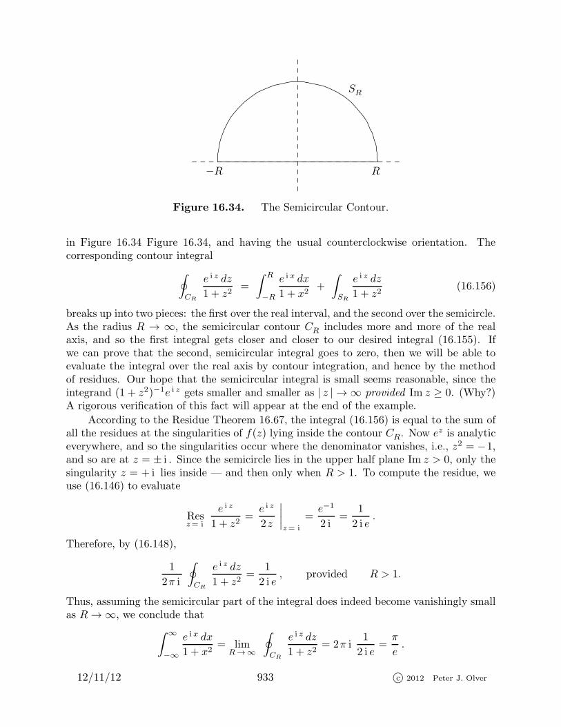
R−R

SR

Figure 16.34. The Semicircular Contour.

in Figure 16.34 Figure 16.34, and having the usual counterclockwise orientation. Thecorresponding contour integral

∮

CR

e i z dz

1 + z2=

∫ R

−R

e ix dx

1 + x2+

∫

SR

e i z dz

1 + z2(16.156)

breaks up into two pieces: the first over the real interval, and the second over the semicircle.As the radius R → ∞, the semicircular contour CR includes more and more of the realaxis, and so the first integral gets closer and closer to our desired integral (16.155). Ifwe can prove that the second, semicircular integral goes to zero, then we will be able toevaluate the integral over the real axis by contour integration, and hence by the methodof residues. Our hope that the semicircular integral is small seems reasonable, since theintegrand (1 + z2)−1e i z gets smaller and smaller as | z | → ∞ provided Im z ≥ 0. (Why?)A rigorous verification of this fact will appear at the end of the example.

According to the Residue Theorem 16.67, the integral (16.156) is equal to the sum ofall the residues at the singularities of f(z) lying inside the contour CR. Now ez is analyticeverywhere, and so the singularities occur where the denominator vanishes, i.e., z2 = −1,and so are at z = ± i . Since the semicircle lies in the upper half plane Im z > 0, only thesingularity z = + i lies inside — and then only when R > 1. To compute the residue, weuse (16.146) to evaluate

Resz= i

e i z

1 + z2=e i z

2z

∣∣∣∣z= i

=e−1

2 i=

1

2 i e.

Therefore, by (16.148),

1

2π i

∮

CR

e i z dz

1 + z2=

1

2 i e, provided R > 1.

Thus, assuming the semicircular part of the integral does indeed become vanishingly smallas R→ ∞, we conclude that

∫ ∞

−∞

e ix dx

1 + x2= lim

R→∞

∮

CR

e i z dz

1 + z2= 2π i

1

2 i e=π

e.

12/11/12 933 c© 2012 Peter J. Olver

Incidentally, the integral is real because its imaginary part,∫ ∞

−∞

sinx dx

1 + x2= 0,

is the integral of an odd function which is automatically zero. Consequently,

I =

∫ ∞

0

cosx dx

1 + x2=

1

2Re

∫ ∞

−∞

e ix dx

1 + x2=

π

2e, (16.157)

which is the desired result.

To complete the argument, let us estimate the size of the semicircular integral. Theintegrand is bounded by

∣∣∣∣e i z

1 + z2

∣∣∣∣ ≤ 1

1 + | z |2 =1

1 +R2whenever | z | = R, Im z ≥ 0,

where we are using the fact that∣∣ e i z

∣∣ = e−y ≤ 1 whenever z = x+ i y with y ≥ 0.

According to Corollary 16.55, the size of the integral of a complex function is boundedby its maximum modulus along the curve times the length of the semicircle, namely πR.Thus, in our case,

∣∣∣∣∫

SR

e i z dz

1 + z2

∣∣∣∣ ≤ πR

1 +R2≤ π

R−→ 0 as R −→ ∞,

as required.

Example 16.72. Here we will use residues to evaluate the real integral∫ ∞

−∞

dx

1 + x4. (16.158)

The indefinite integral can, in fact, be found by the method of partial fractions, but, asyou may know, this is not a particularly pleasant task. Let us try the method of residues.Let CR denote the same semicircular contour as in Figure 16.34. The integrand has polesingularities where the denominator vanishes, i.e., z4 = −1, and so at the four fourth rootsof −1. These are

eπ i /4 =1 + i√

2, e3π i /4 =

−1 + i√2

, e5π i /4 =1− i√

2, e7π i /4 =

−1− i√2

.

Only the first two roots lie inside CR when R > 1. Their residues can be computed using(16.146):

Resz=eπ i /4

1

1 + z4=

1

4z3

∣∣∣∣z=eπ i /4

=e−3π i /4

4=

−1− i

4√2

,

Resz=e3π i /4

1

1 + z4=

1

4z3

∣∣∣∣z=e3π i /4

=e−9π i /4

4=

1− i

4√2.

12/11/12 934 c© 2012 Peter J. Olver

Therefore, by the residue formula (16.148),

∮

CR

dz

1 + z4= 2π i

( −1− i

4√2

+1− i

4√2

)=

π√2. (16.159)

On the other hand, we can break up the contour integral into an integral along thereal axis and an integral around the semicircle:

∮

CR

dz

1 + z4=

∫ R

−R

dx

1 + x4+

∫

SR

dz

1 + z4.

The first integral goes to the desired real integral as the radius R → ∞. On the otherhand, on a large semicircle | z | = R, the integrand is small:

∣∣∣∣1

1 + z4

∣∣∣∣ ≤ 1

1 + | z |4 =1

1 +R4when | z | = R.

Thus, using Corollary 16.55, the integral around the semicircle can be bounded by∣∣∣∣∫

SR

dz

1 + z4

∣∣∣∣ ≤ 1

1 +R4πR ≤ π

R3−→ 0 as R −→ ∞.

Thus, as R→ ∞, the complex integral (16.159) goes to the desired real integral (16.158),and so ∫ ∞

−∞

dx

1 + x4=

π√2.

Note that the result is real and positive, as it must be.

12/11/12 935 c© 2012 Peter J. Olver