Chapter 16

Management of Short-term Assets

Preliminary Definitions

• Working capital: Current (short-term) assets

• Net working capital: Current assets minus current liabilities

• Working capital policy: Management of current assets and current liabilities

The Operating Cycle

• Time it takes to produce output, sell it, and collect payment

• Timing of payments– Varies among industries

– Affects the need for short-term finance

Financing and Working Capital Policy

• Matching sources and uses of funds

• Basic principle: do not use short-term sources to finance long-term assets

• Cost structure of funds:– Long-term sources tend to be more

expensive than short-term source

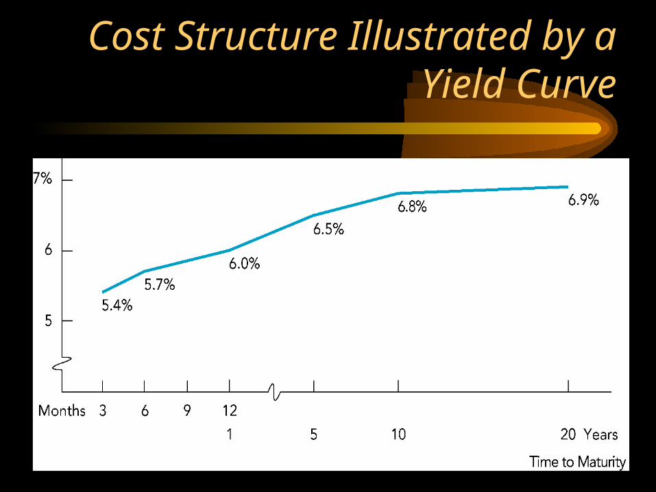
Cost Structure Illustrated by a Yield Curve

Aggressive Working Capital Policy

• Use of more short-term sources– Increases profitability

– Increases risk

• But also increases the need to roll over or refinance short-term debt

Inventory Cycle

• Inventory is– acquired

– drawn down to some level

– replenished

– and the cycle is repeated

• The safety stock

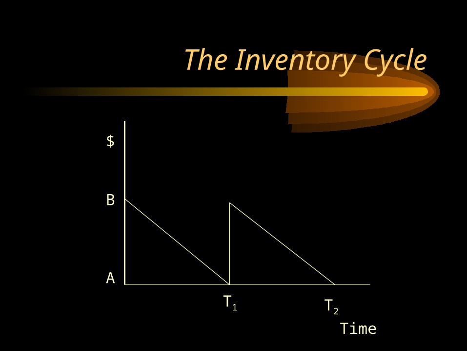
The Inventory Cycle

$

Time

T1

A

B

T2

The Economic Order Quantity (EOQ)

• Ordering costs versus carrying costs

• Fewer orders reduce ordering costs but increases carrying costs

The Economic Order Quantity (EOQ)

• The EOQ minimizes the sum of– Ordering costs (e.g., shipping and

processing costs) plus

– Carrying costs (e.g., warehouse expense, insurance, and interest expense)

The Economic Order Quantity (EOQ)

• EOQ = (2SF/C).5

• EOQ = ((2 x 10,000 x $50)/$10).5 = 316

The Economic Order Quantity (EOQ)

$ Costs

Order Size316

B

Total Ordering Costs

Total Carrying Costs

D

Total Costs

F

C

$3,180

E

A

The Inventory Cycle Combined with the EOQ

Days10

50

366

15

Safety Stock

Level of Inventory

Units of Inventory

0 5

The Inventory Cycle Combined with the EOQ

• Maximum inventory: EOQ plus the safety stock

• Minimum inventory: Safety stock

• Average inventory: EOQ/2 + safety stock

EOQ Model

• A very simple model

• Assumes– sales occur evenly– no quantity discounts– individual items are identifiable

• Highlights the trade off between ordering costs and carrying costs

Just-in-Time inventory management

• Designed to minimize the amount of inventory

• Requires– accurate forecasts– excellent timing– dependable shipping– flexible schedules– frequent communication

Management of Accounts Receivable

• Credit policy encompasses

– Who will receive credit

– Terms of credit

– Collections

Decision to Grant Credit

• Trade-off between additional sales versus additional costs

• Additional costs– Cost of goods sold

– Credit and collection costs

– Bad debt expense

– Carrying costs

Analyzing Accounts Receivable

• Receivables turnover: Credit sales/Accounts receivable

• Aging schedules: Determine payment patterns

Cash Management

• Faster collections

• Slower disbursements

• Investing short-term funds

Facilitating Faster Collections

• Electronic funds transfers

• Lockbox

The Flow of Checks and Funds

Money Market Instruments and Yields the Instruments

• U.S. Treasury bills

• Commercial paper

• Negotiable certificates of deposit

• Banker's acceptances

• Eurodollar CDs

• Repurchase agreements (REPOs)

Yields: the Discount Yield

• Depends on– The principal amount

– The amount of the discount– The time to maturity

Yd = Par value - Price x ________360_______

Par value Number of days to maturity

Yields: the Discount Yield

• Yd = Par value - Price x ________360_______

Par value Number of days to maturity

• $10,000 - $9,791 x _360_ = $10,000 180

4.18%

Yields: the Discount Yield

• Weaknesses– Use of 360 days

– Return based on par value and not price

• Yd = Par value - Price x _ 365______

Price Number of days to maturity

• $10,000 - $9,791 x _365_ = $9,791 180

Alternative Calculation: Simple Interest

4.33%

Alternative Calculation: Compound Interest

• Price(1 + i)t = Face Value

• Example– price: $9,791

face value: $10,000time period: 180 days$9,791(1 + i)0.49315 = $10,000i = (1.02135)2.0278 - 1 = 4.38%