Embed Size (px)
Citation preview
Chapter 15 – Scheduling
Operations Managementby
R. Dan Reid & Nada R. Sanders2nd Edition © Wiley 2005
PowerPoint Presentation by R.B. Clough - UNH
Learning Objectives
Explain the different kinds of scheduling Describe different shop loading methods Develop a schedule using priority rules Calculate scheduling performance measures Develop a schedule for multiple
workstations Describe the theory of constraints Describe scheduling for service applications Develop a workforce schedule in which each
employee has two consecutive days off
Scheduling Definitions Routing:
The operations to be performed, their sequence, the work centers visited, & the time standards
Bottleneck: A resource whose capacity is less than the demand placed on
it Due date:
When the job is supposed to be finished Slack:
The time that a job can be delayed & still finish by its due date Queue:
A waiting line
High-Volume Operations Flow operations like automobiles, bread, gasoline High-volume standard items; discrete or
continuous with smaller profit margins Designed for high efficiency and high utilization High volume flow operations with fixed routings Bottlenecks are easily identified Commonly use line-balancing to design the
process around the required tasks

Low-Volume Operations Low-volume, job shop operations, are
designed for flexibility. Use more general purpose equipment Customized products with higher margins Each product or service may have its own
routing (scheduling is much more difficult) Bottlenecks move around depending upon
the products being produced at any given time
Low-Volume Tool – Gantt Charts
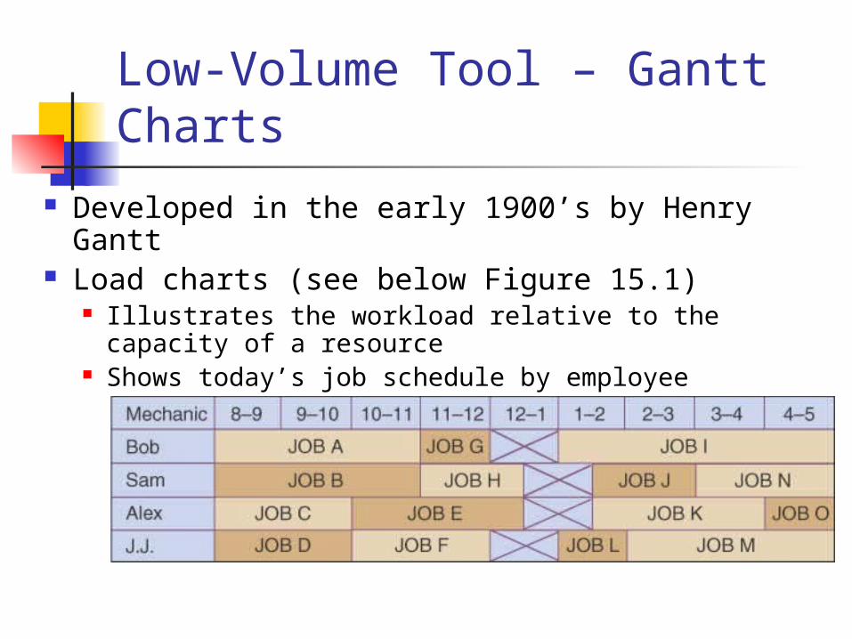
Developed in the early 1900’s by Henry Gantt Load charts (see below Figure 15.1)
Illustrates the workload relative to the capacity of a resource
Shows today’s job schedule by employee
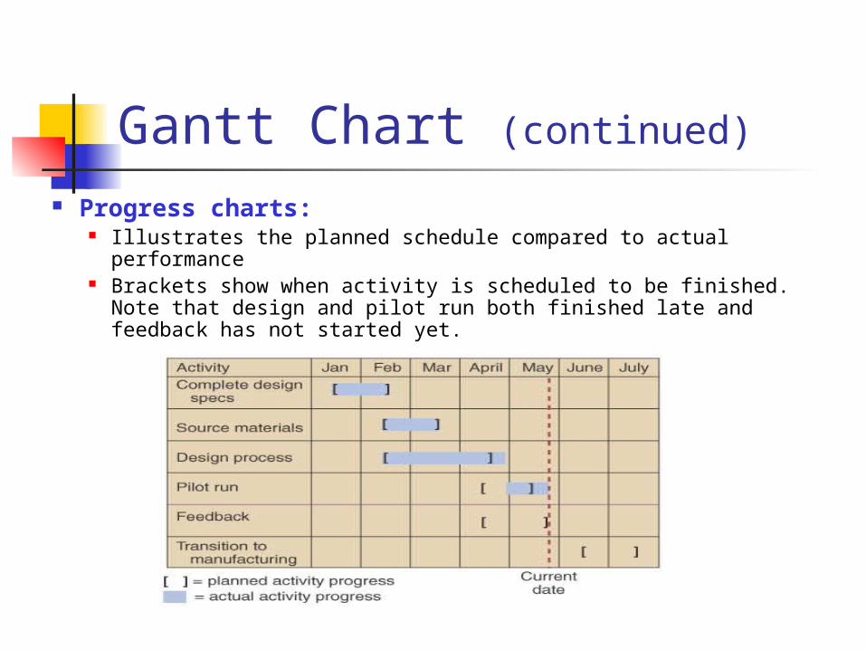
Gantt Chart (continued)
Progress charts: Illustrates the planned schedule compared to actual performance Brackets show when activity is scheduled to be finished. Note
that design and pilot run both finished late and feedback has not started yet.
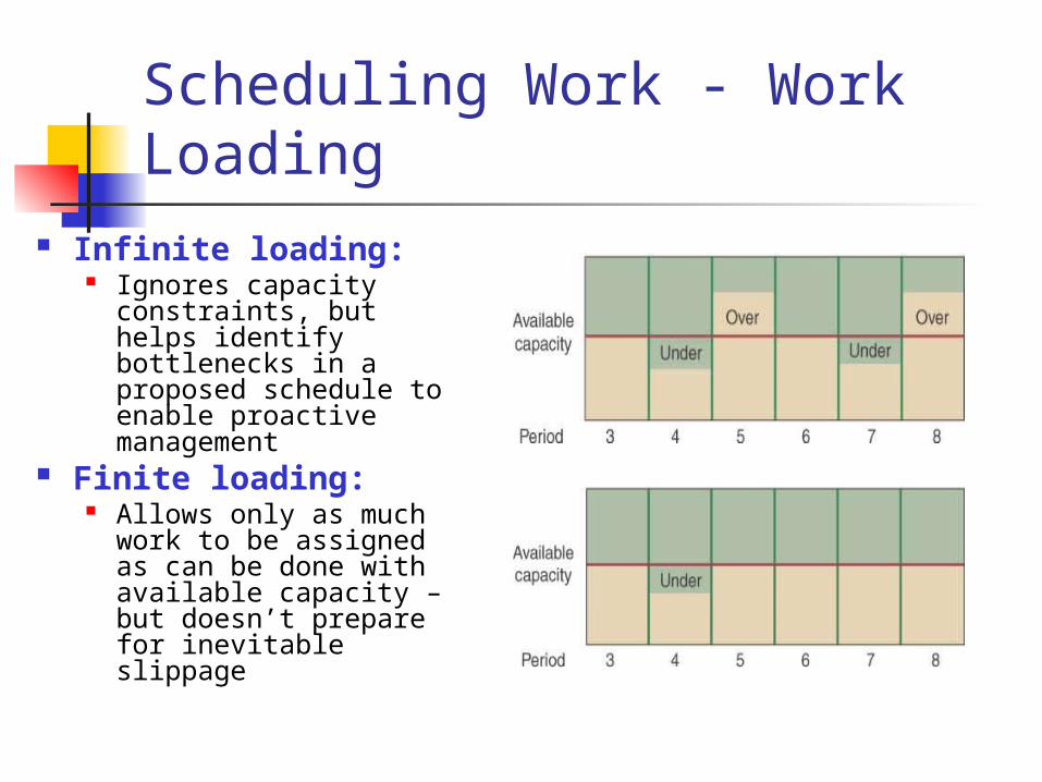
Scheduling Work - Work Loading
Infinite loading: Ignores capacity
constraints, but helps identify bottlenecks in a proposed schedule to enable proactive management
Finite loading: Allows only as much
work to be assigned as can be done with available capacity – but doesn’t prepare for inevitable slippage
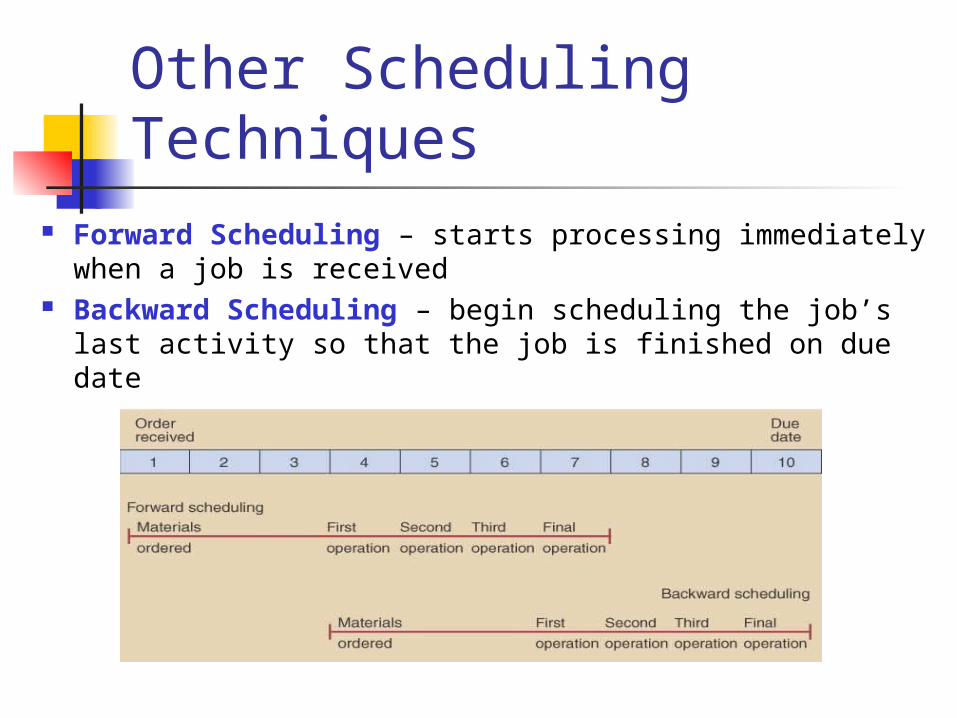
Other Scheduling Techniques
Forward Scheduling – starts processing immediately when a job is received
Backward Scheduling – begin scheduling the job’s last activity so that the job is finished on due date
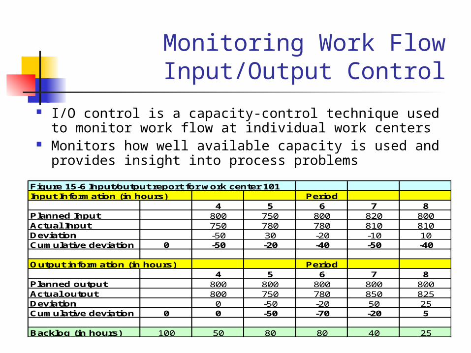
Monitoring Work Flow Input/Output Control
I/O control is a capacity-control technique used to monitor work flow at individual work centers
Monitors how well available capacity is used and provides insight into process problems
Figure 15-6 Input/output report for work center 101Input Information (in hours) Period
4 5 6 7 8Planned Input 800 750 800 820 800Actual Input 750 780 780 810 810Deviation -50 30 -20 -10 10Cumulative deviation 0 -50 -20 -40 -50 -40
Output information (in hours) Period4 5 6 7 8
Planned output 800 800 800 800 800Actual output 800 750 780 850 825Deviation 0 -50 -20 50 25Cumulative deviation 0 0 -50 -70 -20 5
Backlog (in hours) 100 50 80 80 40 25
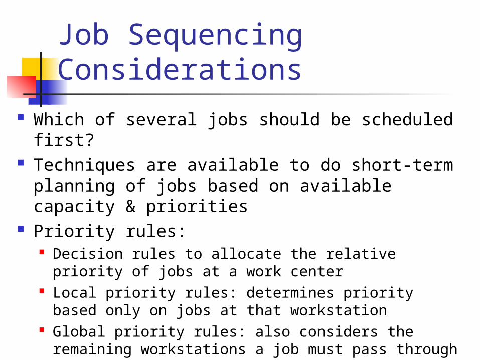
Job Sequencing Considerations
Which of several jobs should be scheduled first? Techniques are available to do short-term
planning of jobs based on available capacity & priorities
Priority rules: Decision rules to allocate the relative priority of jobs
at a work center Local priority rules: determines priority based only
on jobs at that workstation Global priority rules: also considers the remaining
workstations a job must pass through
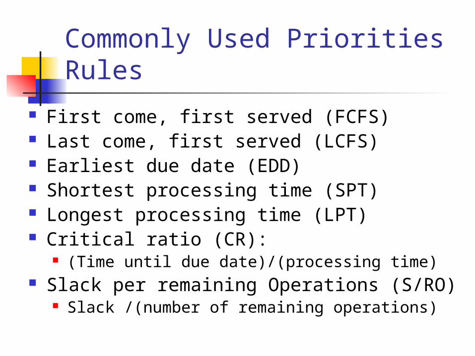
Commonly Used Priorities Rules
First come, first served (FCFS) Last come, first served (LCFS) Earliest due date (EDD) Shortest processing time (SPT) Longest processing time (LPT) Critical ratio (CR):
(Time until due date)/(processing time) Slack per remaining Operations (S/RO)
Slack /(number of remaining operations)
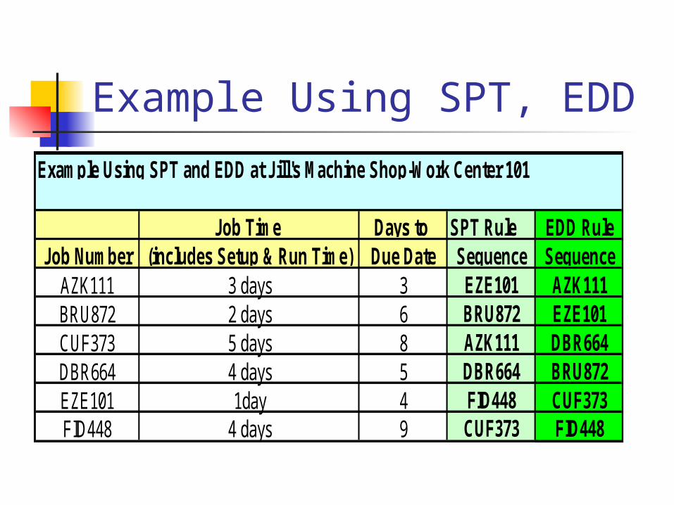
Example Using SPT, EDD
Example Using SPT and EDD at Jill's Machine Shop-Work Center 101
Job Time Days to SPT Rule EDD RuleJob Number (includes Setup & Run Time) Due Date Sequence Sequence
AZK111 3 days 3 EZE101 AZK111BRU872 2 days 6 BRU872 EZE101CUF373 5 days 8 AZK111 DBR664DBR664 4 days 5 DBR664 BRU872EZE101 1day 4 FID448 CUF373FID448 4 days 9 CUF373 FID448
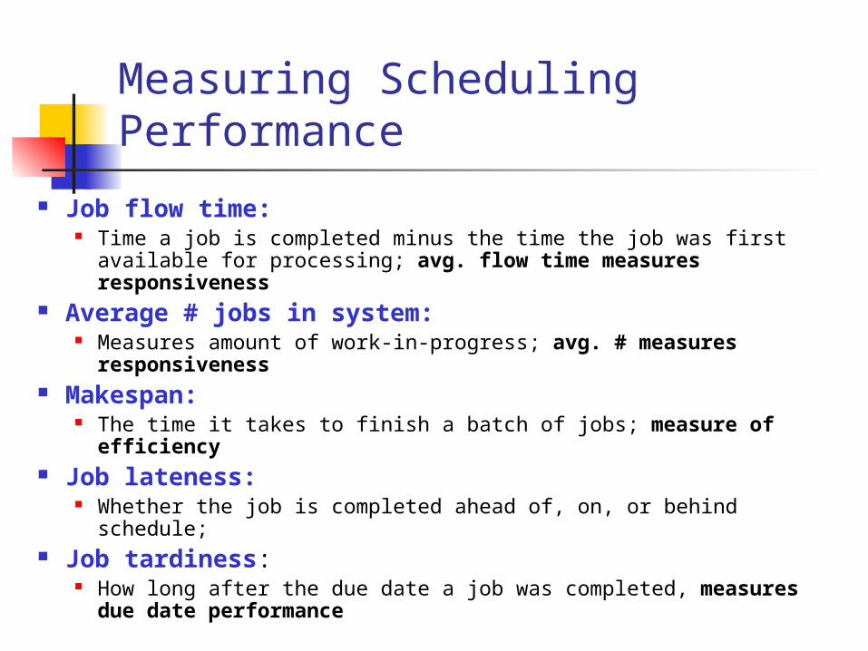
Measuring Scheduling Performance
Job flow time: Time a job is completed minus the time the job was first
available for processing; avg. flow time measures responsiveness
Average # jobs in system: Measures amount of work-in-progress; avg. # measures
responsiveness Makespan:
The time it takes to finish a batch of jobs; measure of efficiency
Job lateness: Whether the job is completed ahead of, on, or behind schedule;
Job tardiness: How long after the due date a job was completed, measures
due date performance
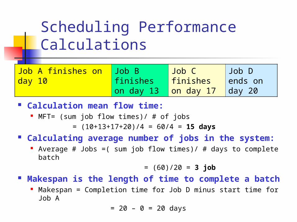
Scheduling Performance Calculations
Calculation mean flow time: MFT= (sum job flow times)/ # of jobs = (10+13+17+20)/4 = 60/4 = 15 days
Calculating average number of jobs in the system: Average # Jobs =( sum job flow times)/ # days to complete batch = (60)/20 = 3 job
Makespan is the length of time to complete a batch
Makespan = Completion time for Job D minus start time for Job A = 20 – 0 = 20 days
Job A finishes on day 10
Job B finishes on day 13
Job C finishes on day 17
Job D ends on day 20
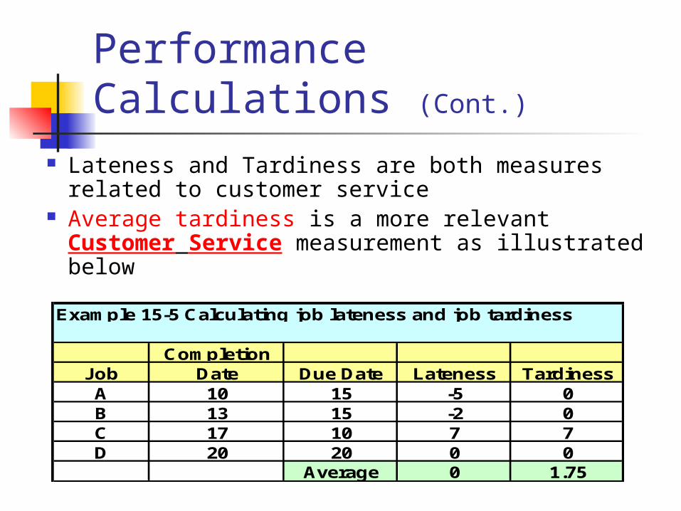
Performance Calculations (Cont.)
Lateness and Tardiness are both measures related to customer service
Average tardiness is a more relevant Customer Service measurement as illustrated below
Example 15-5 Calculating job lateness and job tardiness
CompletionJob Date Due Date Lateness TardinessA 10 15 -5 0B 13 15 -2 0C 17 10 7 7D 20 20 0 0
Average 0 1.75
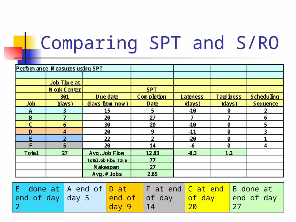
Comparing SPT and S/RO
E done at end of day 2
A end of day 5
D at end of day 9
F at end of day 14
C at end of day 20
B done at end of day 27
Performance Measures using SPT
Job Time atWork Center SPT
301 Due date Completion Lateness Tardiness Scheduling Job (days) (days from now) Date (days) (days) SequenceA 3 15 5 -10 0 2B 7 20 27 7 7 6C 6 30 20 -10 0 5D 4 20 9 -11 0 3E 2 22 2 -20 0 1F 5 20 14 -6 0 4
Total 27 Avg. Job Flow 12.83 -8.3 1.2Total Job Flow Time 77
Makespan 27Avg. # Jobs 2.85
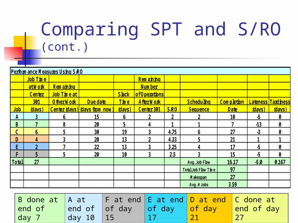
Comparing SPT and S/RO (cont.)
Performance Measures Using S/ROJob Time Remainingat Work Remaining Number Center Job Time at Slack of Operations
301 Other Work Due date Time After Work Scheduling Completion Lateness TardinessJob (days) Center (days) (days from now) (days) Center 301 S/RO Sequence Date (days) (days)A 3 6 15 6 2 2 2 10 -5 0B 7 8 20 5 4 1 1 7 -13 0C 6 5 30 19 3 4.75 6 27 -3 0D 4 3 20 13 2 4.33 5 21 1 1E 2 7 22 13 3 3.25 4 17 -5 0F 5 5 20 10 3 2.5 3 15 -5 0
Total 27 Avg. Job Flow 16.17 -5.0 0.167Total Job Flow Time 97
Makespan 27Avg. # Jobs 3.59
B done at end of day 7
A at end of day 10
F at end of day 15
E at end of day 17
D at end of day 21
C done at end of day 27
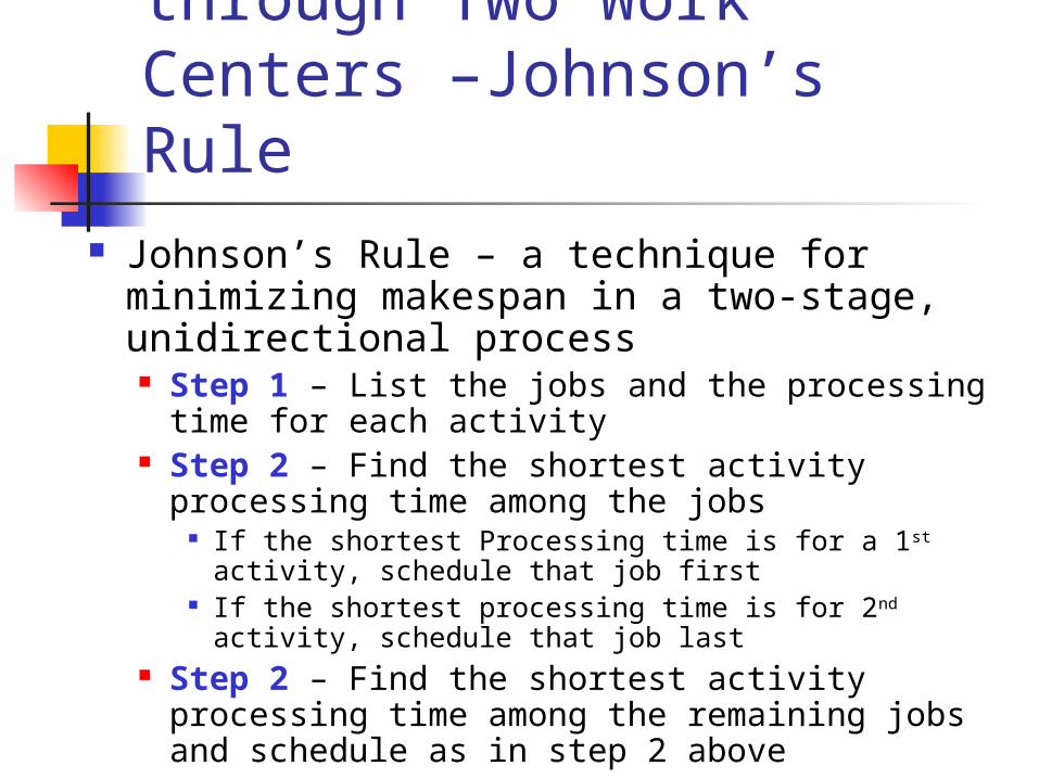
Sequencing Jobs through Two Work Centers –Johnson’s Rule
Johnson’s Rule – a technique for minimizing makespan in a two-stage, unidirectional process Step 1 – List the jobs and the processing time
for each activity Step 2 – Find the shortest activity processing
time among the jobs If the shortest Processing time is for a 1st activity,
schedule that job first If the shortest processing time is for 2nd activity,
schedule that job last Step 2 – Find the shortest activity processing
time among the remaining jobs and schedule as in step 2 above
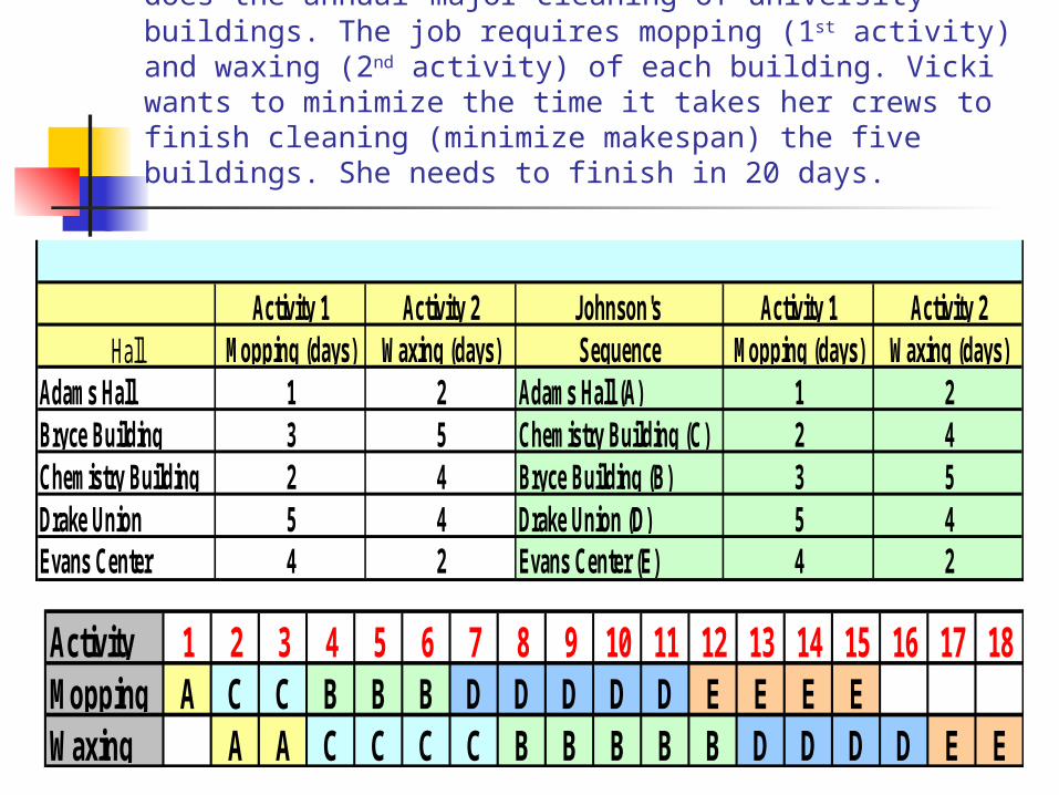
Johnson’s Rule Example: Vicki’s Office Cleaners does the annual major cleaning of university buildings. The job requires mopping (1st activity) and waxing (2nd activity) of each building. Vicki wants to minimize the time it takes her crews to finish cleaning (minimize makespan) the five buildings. She needs to finish in 20 days.
Activity 1 Activity 2 Johnson's Activity 1 Activity 2Hall Mopping (days) Waxing (days) Sequence Mopping (days) Waxing (days)
Adams Hall 1 2 Adams Hall (A) 1 2Bryce Building 3 5 Chemistry Building (C) 2 4Chemistry Building 2 4 Bryce Building (B) 3 5Drake Union 5 4 Drake Union (D) 5 4Evans Center 4 2 Evans Center (E) 4 2
Activity 1 2 3 4 5 6 7 8 9 10 11 12 13 14 15 16 17 18Mopping A C C B B B D D D D D E E E EWaxing A A C C C C B B B B B D D D D E E
Scheduling Bottlenecks - OPT
In the 1970’s Eli Goldratt introduced optimized production technology
OPT focused on bottlenecks for scheduling & capacity planning
Definitions: Throughput: quantity of finished goods that can be
sold Process batch: quantity produced at a resource
before switching to another product Transfer batch: quantity routed at one time from
one resource to the next
OPT Principles Balance the process rather than the flow Non-bottleneck usage is driven by some other
constraint in the system Use and activation of a resource are not the same A hour lost at a bottleneck is lost forever, but an
hour lost at a non-bottleneck is a mirage Bottleneck determine throughput and inventory in
system The transfer batch does not need to be equal to the
process batch The process batch should be variable Consider all constraints simultaneously. Lead times
are the result of the schedule and are not predetermined .
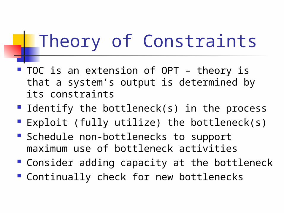
Theory of Constraints TOC is an extension of OPT – theory is that a
system’s output is determined by its constraints
Identify the bottleneck(s) in the process Exploit (fully utilize) the bottleneck(s) Schedule non-bottlenecks to support
maximum use of bottleneck activities Consider adding capacity at the bottleneck Continually check for new bottlenecks
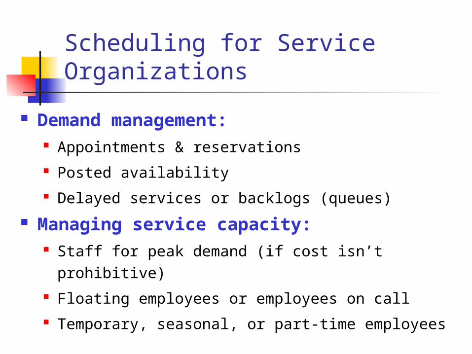
Scheduling for Service Organizations
Demand management: Appointments & reservations Posted availability Delayed services or backlogs (queues)
Managing service capacity: Staff for peak demand (if cost isn’t prohibitive) Floating employees or employees on call Temporary, seasonal, or part-time employees
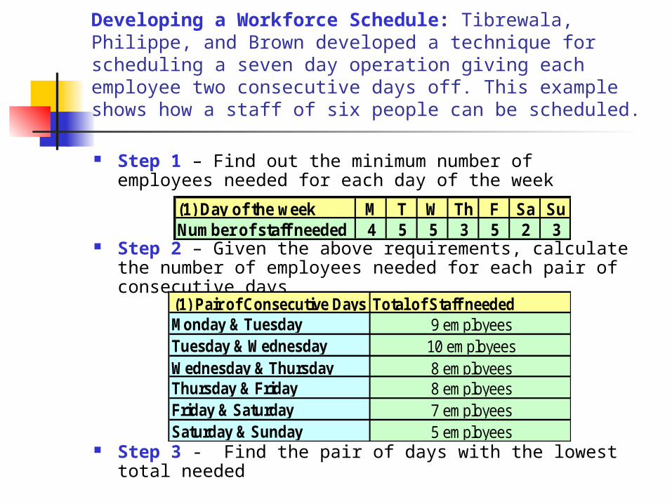
Developing a Workforce Schedule: Tibrewala, Philippe, and Brown developed a technique for scheduling a seven day operation giving each employee two consecutive days off. This example shows how a staff of six people can be scheduled.
Step 1 – Find out the minimum number of employees needed for each day of the week
Step 2 – Given the above requirements, calculate the number of employees needed for each pair of consecutive days
Step 3 - Find the pair of days with the lowest total needed
(1) Day of the week M T W Th F Sa SuNumber of staff needed 4 5 5 3 5 2 3
(1) Pair of Consecutive Days Total of Staff neededMonday & Tuesday 9 employeesTuesday & Wednesday 10 employeesWednesday & Thursday 8 employeesThursday & Friday 8 employeesFriday & Saturday 7 employeesSaturday & Sunday 5 employees
Workforce Scheduling (cont.)
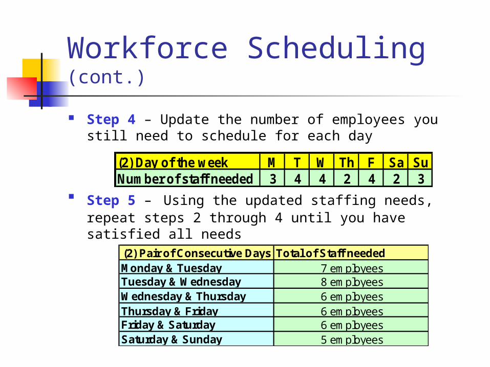
Step 4 – Update the number of employees you still need to schedule for each day
Step 5 – Using the updated staffing needs, repeat steps 2 through 4 until you have satisfied all needs
(2) Day of the week M T W Th F Sa SuNumber of staff needed 3 4 4 2 4 2 3
(2) Pair of Consecutive Days Total of Staff neededMonday & Tuesday 7 employeesTuesday & Wednesday 8 employeesWednesday & Thursday 6 employeesThursday & Friday 6 employeesFriday & Saturday 6 employeesSaturday & Sunday 5 employees
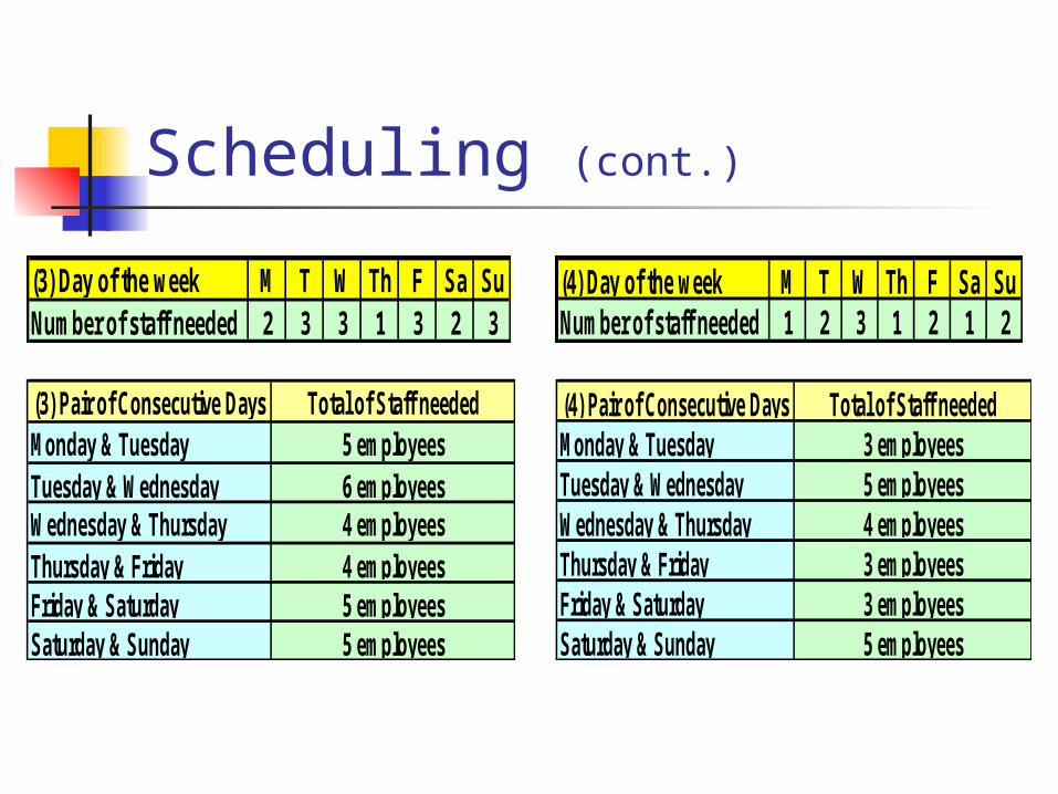
Scheduling (cont.)
(3) Pair of Consecutive Days Total of Staff neededMonday & Tuesday 5 employeesTuesday & Wednesday 6 employeesWednesday & Thursday 4 employeesThursday & Friday 4 employeesFriday & Saturday 5 employeesSaturday & Sunday 5 employees
(4) Pair of Consecutive Days Total of Staff neededMonday & Tuesday 3 employeesTuesday & Wednesday 5 employeesWednesday & Thursday 4 employeesThursday & Friday 3 employeesFriday & Saturday 3 employeesSaturday & Sunday 5 employees
(3) Day of the week M T W Th F Sa SuNumber of staff needed 2 3 3 1 3 2 3
(4) Day of the week M T W Th F Sa SuNumber of staff needed 1 2 3 1 2 1 2
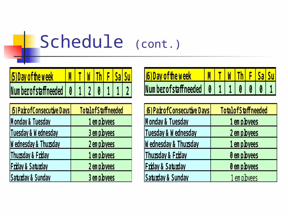
Schedule (cont.)
(5) Day of the week M T W Th F Sa SuNumber of staff needed 0 1 2 0 1 1 2
(6) Pair of Consecutive Days Total of Staff neededMonday & Tuesday 1 employeesTuesday & Wednesday 2 employeesWednesday & Thursday 1 employeesThursday & Friday 0 employeesFriday & Saturday 0 employeesSaturday & Sunday 1 employees
(5) Pair of Consecutive Days Total of Staff neededMonday & Tuesday 1 employeesTuesday & Wednesday 3 employeesWednesday & Thursday 2 employeesThursday & Friday 1 employeesFriday & Saturday 2 employeesSaturday & Sunday 3 employees
(6) Day of the week M T W Th F Sa SuNumber of staff needed 0 1 1 0 0 0 1

Final Schedule
(7) Day of the week M T W Th F Sa SuNumber of staff needed 0 0 0 0 0 0 0
Employees M T W Th F Sa Su1 x x x x x off off2 x x x x x off off3 x x off off x x x4 x x x x x off off5 off off x x x x x6 x x x x off off x
This technique gives a work schedule for each employee to satisfy minimum daily staffing requirements
Next step is to replace numbers with employee names
Manager can give senior employees first choice and proceed until all employees have a schedule
Chapter 15 Highlights Scheduling techniques depend on volume. High volume
is typically done through line design and balancing. Low volume uses priority rules along with visual techniques like Gantt charts.
Shop loading can assume infinite or finite loading which is constrained by predetermined capacity. Loading can be done by using forward or backward scheduling.
Scheduling decisions use common priority rules like SPT, EDD, FCFS, and S/RO. Priority rules need to support organizational objectives.
Performance measures like mean flow time, job lateness, job tardiness, makespan, and the average number of jobs in the system measure the effectiveness of schedules.
Chapter 15 Highlights John’s Rule is a effective technique for minimizing
makespan when successive workstations are needed to complete the process.
OPT principles can be used to schedule bottlenecks. TOC expands OPT into a continuous improvement philosophy.
Service organizations use different techniques such as appointments, reservations, and posted schedules for use of service capacity.
Techniques exist for workforce scheduling when a company uses full time employees, operates 7 days each week, and gives its employees 2 consecutive days off.
The End Copyright © 2005 John Wiley & Sons, Inc. All rights
reserved. Reproduction or translation of this work beyond that permitted in Section 117 of the 1976 United State Copyright Act without the express written permission of the copyright owner is unlawful. Request for further information should be addressed to the Permissions Department, John Wiley & Sons, Inc. The purchaser may make back-up copies for his/her own use only and not for distribution or resale. The Publisher assumes no responsibility for errors, omissions, or damages, caused by the use of these programs or from the use of the information contained herein.