Chapter 15 MSM2M2 Introduction To Management …igor.gold.ac.uk/~mas01rwb/notes/2M2.pdfMSM2M2 Introduction To Management Mathematics ... a simpliﬁed form of it — its ‘O’ set

Chapter 15

MSM2M2 Introduction To Management

Mathematics

(15.1) Combinatorial Methods

(15.1.1) Algorithms & Complexity

At the heart of any combinatorial method is an algorithm; a process which is (supposed) to yield the mostefficient or profitable solution so some situation. A simple and obvious way to do this is as follows. In anattempt to solve this, the following could be used.

Algorithm 1 (The Greedy Algorithm) Choose the most attractive feasible option available.

However, it is easy to construct situations where this does not work — a number of conditions about theproblem must be satisfied in order the the Greedy Algorithm to work. In search of a better solution to theone supplied using the Greedy Algorithm, it may be possible to find all permutations then choose the best.However, even powerful computers may not be able to solve even simple problems given many years. Twoareas of interest are apparent,

• does a given algorithm find a correct solution.

• how efficient is the algorithm.

In a mathematical sense, the efficiency can be expressed in terms of how many elementary operations —addition, multiplication, etc. — must be performed in order to achieve the result. However, the ‘input’ mustalso be taken into account as clearly an algorithm that takes 10 operations on 3 ‘inputs’ is less efficient thanone that takes 10 operations on 30 ‘inputs’.

Example 2 Compute the number of elementary operations needed to evaluate the polynomial function p(x) = anxn +an−1xn−1 + · · ·+ a1x + a0 using the method

1. by calculating the powers of x, multiplying by the coefficient ai, then adding the terms.

2. by starting with the lowest power of x, and ‘saving’ the powers of x for use in calculating the next term, thenadding the terms.

3. using Horner’s Method, p(x) = (. . . ((anx + an−1) x + an−2) x + · · ·+ a1) x + a0

Proof. Solution

1. Evaluation using this method involves

1

2 CHAPTER 15. MSM2M2 MANAGEMENT MATHEMATICS

• i − 1 multiplications for the power of x in the ith term and another for the coefficient, giving a

total ofn∑

i=0i = 1

2 n(n + 1).

• n additions in order to combine the resulting n + 1 terms.

This gives a total of 12 n(n + 1) + n = 1

2 n2 + 32 n.

2. Evaluation using this method involves

• The term with x0 requires no multiplication. The term with x1 requires one multiplication, thecoefficient. Subsequent terms require a multiplication by x and by the coefficient i.e. two each.There are therefore 0 + 1 + 2(n− 2) = 2n− 1 multiplications.

• n additions in order to combine the n + 1 terms.

This gives a total of 3n− 1.

3. Evaluation using Horner’s method involves

• one multiplication for each power of x — these are the xs outside the brackets of which thereare n− 1 and the ‘first’ x which is multiplied by its coefficient, giving n multiplications.

• whenever an x appears it is multiplied by something then added to the next coefficient. Thereare therefore n additions.

This gives a total of 2n operations performed. �

Finding the number of operations is easy enough in this case, and the number of ‘inputs’ — n + 2 — isobvious. What is not obvious, though, is how to combine the two.

Definition 3 The computational complexity of an algorithm A, cc(A), is the number of operations performed on aninput of length L. This is expressed as a function of L so that cc(A) = f (L).

In Example ( 2 ) the computational complexities can now be calculated and are

1. (L−2)2

2 + 3(L−2)2 .

2. 3L− 7.

3. 2L− 4.

Clearly Horner’s method is the most efficient for an input of any given length.

Functions for the computational complexity may vary enormously for the same result but using differentprocesses. It is of course desirable to achieve the computational complexity of lowest value. This is typicallydone by reducing the power of the expression, or in the linear case by reducing the values of the coefficients.

(15.1.2) ‘O’ Notation

It is convenient at this point to introduce the apparently bizarre ‘ ‘O’ notation’. Consider the set of realfunctions defined on R+ which are eventually positive, i.e.

F+ ={

f | f : R+ → R with f (x) > 0 ∀x > x0, x0 ∈ R+}For g(x) ∈ F+ the following definition is now made.

Definition 4 The function O(g) for a function g which is eventually positive i.e. g ∈ F+ is given by the set

O(g) ={

f (x) ∈ F+ | ∃c > 0 ∃x0 > 0 ∀x > x0 f (x) 6 c× g(x)}

15.1. COMBINATORIAL METHODS 3

Note that when f ∈ O(g) it is common to write “ f = O(g)” or even “ f (x) = (g(x))”. O(g) is the eventuallypositive functions whose value at x does not exceed c times g(x), eventually. It is readily deduced that.Iff (x) 6 g(x) then O( f ) ⊆ O(g), i.e. f = O(g). As functions can be composed, it follows that some similarprocess can be performed on the sets O.

Definition 5

1. O( f ) + O(g) ={

f (x) + g(x) | f ∈ O( f ) and g ∈ O(g)}

2. O( f ) ·O(g) ={

f (x) · g(x) | f ∈ O( f ) and g ∈ O(g)}

3. f + O(g) = { f (x) + g(x) | g ∈ O(g)}

4. f ·O(g) = { f (x) · g(x) | g ∈ O(g)}

The abuse of notation “ f (x) = (g(x))” is extended so that “⊆” becomes the same as “6”. It is readily shownfrom the definition that if f ∈ O(g) then O( f ) 6 O(g), and indeed if f 6 g then O( f ) 6 O(g). Along the sameline of thought, the following can be shown from the definitions above.

Theorem 6 For f , g ∈ F+ and k ∈ R+,

1. O( f + g) = O( f ) + O(g)

2. O( f · g) = O( f ) ·O(g)

3. k ·O( f ) = O( f )

4. g 6 f ⇒ O(g + f ) = O( f )

5. g 6 f ⇒ g + O( f ) = O( f )

6. f (x) > ε > 0 ∀x > x0 ⇒ f + a ∈ O( f ) (a > 0)

The virtue of ‘O’ notation can be seen when considering computational complexity functions. Rather thanthe actual function, a simplified form of it — its ‘O’ set — is usually of interest as it gives an indication ofthe level of complexity. For Example 2,

• O(

(L−2)2

2 + 3(L−2)2

)= L2.

• O(3L) = L.

• O(2L) = L.

So while Horner’s method is the simplest, its computational complexity is comparable to that of the secondmethod, while the first method is particularly more complex.

(15.1.3) Sorting

A particular class of algorithm relate to sorting, perhaps most commonly putting a sequence of numbersinto ascending order. First of all the Merge operation is defined.

Definition 7 Suppose that(

x1, x2, . . . , xp)

and(y1, y2, . . . , yq

)are sequences which are already sorted. The Merge

operation defines the sequence(z1, z2, . . . , zp+q

)as follows.

1. If x1 6 y1 then set z1 := x1. Repeat comparing the first elements of(

x2, x3, . . . , xp)

and(y1, y2, . . . , yq

).

2. If x1 > x1 then set z1 := y1. Repeat comparing the first elements of(

x1, x2, . . . , xq)

and(y2, y3, . . . , yp

).


3. The process terminates when one of the sequences becomes empty. The remainder of the other sequence is thencopied onto the end of the new sequence to give

(z1, z2, . . . , zp+q

)In mathematical formulae, merge will be denoted by the binary operation symbol ‘◦’.

The Merge operation takes two elementary operations for each iteration, of which there is one for everyelement of both of the sequences being merged. In the worst case p = q, so since the final element is copied,the computational complexity of Merge must be 2(p + q− 1).Merging can only be done on sorted sequences, which begs the question as to how to sort.

Algorithm 8 (MergeSort) Take an unsorted set of elements, treat each element as a sequence and apply Merge onpairs of the single element sequences. Repeat applying Merge until a single sorted sequence is obtained.

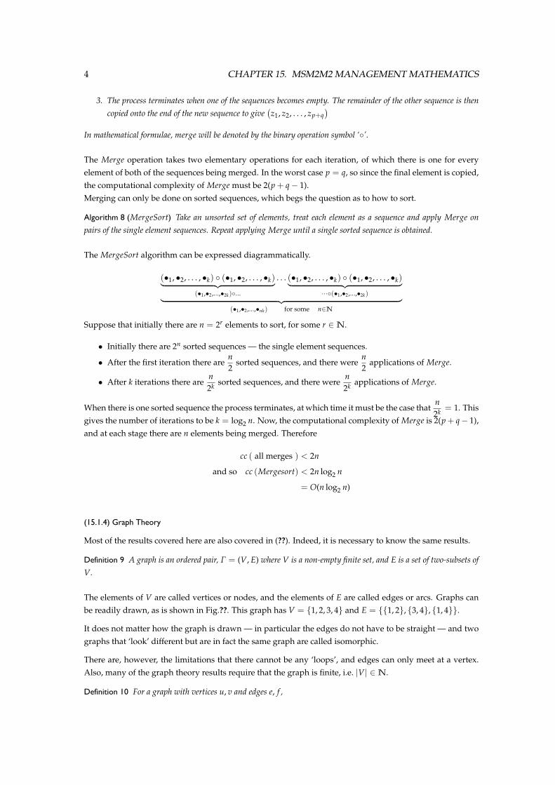
The MergeSort algorithm can be expressed diagrammatically.

(•1, •2, . . . , •k) ◦ (•1, •2, . . . , •k)︸︷︷︸(•1,•2,...,•2k)◦...

. . . (•1, •2, . . . , •k) ◦ (•1, •2, . . . , •k)︸︷︷︸···◦(•1,•2,...,•2k)︸︷︷︸

(•1,•2,...,•nk) for some n∈N

Suppose that initially there are n = 2r elements to sort, for some r ∈ N.

• Initially there are 2n sorted sequences — the single element sequences.

• After the first iteration there aren2

sorted sequences, and there weren2

applications of Merge.

• After k iterations there aren2k sorted sequences, and there were

n2k applications of Merge.

When there is one sorted sequence the process terminates, at which time it must be the case thatn2k = 1. This

gives the number of iterations to be k = log2 n. Now, the computational complexity of Merge is 2(p + q− 1),and at each stage there are n elements being merged. Therefore

cc ( all merges ) < 2n

and so cc (Mergesort) < 2n log2 n

= O(n log2 n)

(15.1.4) Graph Theory

Most of the results covered here are also covered in (??). Indeed, it is necessary to know the same results.

Definition 9 A graph is an ordered pair, Γ = (V, E) where V is a non-empty finite set, and E is a set of two-subsets ofV.

The elements of V are called vertices or nodes, and the elements of E are called edges or arcs. Graphs canbe readily drawn, as is shown in Fig.??. This graph has V = {1, 2, 3, 4} and E = {{1, 2}, {3, 4}, {1, 4}}.

It does not matter how the graph is drawn — in particular the edges do not have to be straight — and twographs that ‘look’ different but are in fact the same graph are called isomorphic.

There are, however, the limitations that there cannot be any ‘loops’, and edges can only meet at a vertex.Also, many of the graph theory results require that the graph is finite, i.e. |V| ∈ N.

Definition 10 For a graph with vertices u, v and edges e, f ,


• if u is one of the vertices at the end of e, then e is incident with u.

• u and v are adjacent if the edge {u, v} is in Γ.

• e and f are adjacent if they are incident with the same vertex.

Definition 11 For a graph Γ = (V, E) with |V| = n and |E| = m then,

• Γ is complete if any vertex is adjacent with any other vertex. Such a graph is written Kn, and clearly m =n∑

i=1i =

n(n− 1)2

.

• Γ is trivial if m = 0 i.e. E = ∅.

• Γ is sparse if m = O(n). If Γ is not sparse then it is dense.

Some such graphs are shown in Fig.2

r rr r�

��

@@

@@

K4

r rr r�

��

A sparse graphr r r�

��

rH

HH

HH

HHH

r r�

��

�A dense graph

Figure 2: Different kinds of graph

Clearly complete graphs are dense.

Definition 12 A graph Γ = (V, E) is bipartite if there exists V1 ⊆ V and V2 ⊆ V, both of which are non-empty, suchthat V1 ∩V2 = ∅, V1 ∪V2 = V and no two vertices of V1 are adjacent and no two vertices of V2 are adjacent.

A complete bipartite graph — where all vertices of V1 are connected to all vertices of V2 but no vertices inV1 — is denoted as Kpq where |V1| = p and |V2| = q.

Definition 13 A graph Γ′ = (V′, E′) is a subgraph of the graph Γ = (V, E) if V′ ⊆ V and E′ ⊆ E. It is common towrite Γ′ ⊆ Γ.

Definition 14 The degree of a vertex is the number of edges incident with that vertex.

So if Γ = (V, E) and v ∈ V then degΓ v = |{u | {u, v} ∈ E}|. Since each edge is incident with exactly twovertices, it is ‘obvious’ that ∑

v∈Vdeg v = 2|E|. A formal proof can be given by induction, or by considering

the incidence matrix of a graph.

Definition 15 For a graph Γ = (V, E), a path in Γ is a sequence of vertices (v1, v2, . . . , vk) such that vi is adjacent tovi+1 for 1 6 i 6 k− 1, and vi 6= vj ∀i 6= j.

Informally put, a path is a sequence of distinct non-adjacent vertices. A ‘u–v path’ is a path which starts atu and ends at v. A graph is called connected if there is a u–v path for all u, v ∈ V.

Definition 16 A cycle is a path (v1, v2, . . . , vk) for which k > 3 and v1 = vk.

A graph with no cycles is called acyclic, and a connected acyclic graph is a tree.

Theorem 17 If Γ is a tree, then there is at least one vertex which has degree 1.


An equivalent to this theorem is to say that if all vertex degrees are at least 2, then Γ contains a cycle, andindeed the proofs are to all intents and purposes, ‘the same’.

Proof. Suppose that the result is false, so that Γ is a tree and all vertex degrees are at least 2.Consider the path of longest length, say P = (v1, v2, . . . , vk) which must exist since Γ is a finite graph.Since deg vk > 2 there must exist some vertex vi 6= vk−1 which is adjacent to vk.But since P was the path of longest length, it must be the case that ∃j < k − 1 such that vi = vj and hence(vi, vi+1, . . . , vk, vi is a cycle in Γ.Contradiction since Γ is a graph. �

Theorem 18 If a graph Γ = (V, E) is a tree, then |E| = |V| − 1.

Proof. The result clearly holds when |V| = 1.Suppose that |V| > 1 and that the result holds.Consider adding a vertex v to Γ to give the graph Γ∗. In order not to create a cycle and hence maintain thestatus of the graph as a tree, v must be connected to Γ by exactly one edge. Observe that

|E| = |V| − 1

|E∗| − 1 = (|V∗| − 1)− 1

|E∗| = |V∗| − 1

So Γ∗ is a tree and the property holds. �

The following extension to Theorem 17 can now be made.

Theorem 19 If Γ = (V, E) is a tree, then at least two vertices have degree 1.

Proof. Suppose the result is false.

If no vertices have degree 1, then since Γ is a tree it must be connected so all vertices have degree at least 2.This contradicts Theorem 17.

The remaining case is that one vertex, say u, has degree 1, and all others have degree at least 2.For the vertices of degree at least 2,

∑v ∈ Vv 6= u

deg v > 2 |V \ {u}|

2|E| > 2 |V \ {u}|

> 2 (|V| − 1)

|E| > |V| − 1

However, this excluded the vertex of degree 1. Adding this in,

|E|+ 1 > |V| − 1

|E| > |V|

But this is a contradiction since by Theorem 18 |E| = |V| − 1. Hence Γ is not a tree, and hence by contradic-tion the theorem must hold. �


So far it has been implicit that all the vertices of the graph are connected together by edges in some way.However, this need not be the case, as a graph may have many different connected component.

Definition 20 A graph Γ1 is a connected component of the graph Γ if

• Γ1 is a subgraph of Γ.

• Γ1 is connected.

• Γ1 is a subgraph of Γ2 is a subgraph of Γ, then Γ1 = Γ2.

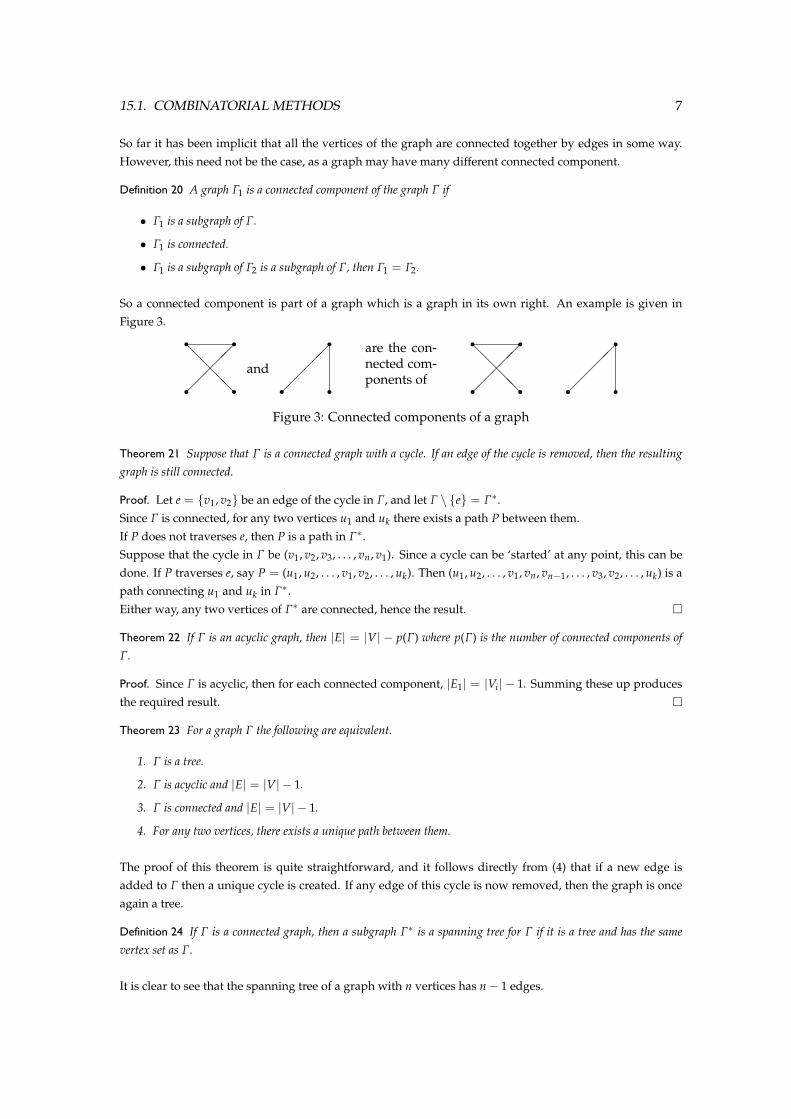
So a connected component is part of a graph which is a graph in its own right. An example is given inFigure 3.

r��

r@

@@@

r rand r��

��

rr are the con-

nected com-ponents of r r �

��

r r@

@@@

r�

��

r r

Figure 3: Connected components of a graph

Theorem 21 Suppose that Γ is a connected graph with a cycle. If an edge of the cycle is removed, then the resultinggraph is still connected.

Proof. Let e = {v1, v2} be an edge of the cycle in Γ, and let Γ \ {e} = Γ∗.Since Γ is connected, for any two vertices u1 and uk there exists a path P between them.If P does not traverses e, then P is a path in Γ∗.Suppose that the cycle in Γ be (v1, v2, v3, . . . , vn, v1). Since a cycle can be ‘started’ at any point, this can bedone. If P traverses e, say P = (u1, u2, . . . , v1, v2, . . . , uk). Then (u1, u2, . . . , v1, vn, vn−1, . . . , v3, v2, . . . , uk) is apath connecting u1 and uk in Γ∗.Either way, any two vertices of Γ∗ are connected, hence the result. �

Theorem 22 If Γ is an acyclic graph, then |E| = |V| − p(Γ) where p(Γ) is the number of connected components ofΓ.

Proof. Since Γ is acyclic, then for each connected component, |E1| = |Vi| − 1. Summing these up producesthe required result. �

Theorem 23 For a graph Γ the following are equivalent.

1. Γ is a tree.

2. Γ is acyclic and |E| = |V| − 1.

3. Γ is connected and |E| = |V| − 1.

4. For any two vertices, there exists a unique path between them.

The proof of this theorem is quite straightforward, and it follows directly from (4) that if a new edge isadded to Γ then a unique cycle is created. If any edge of this cycle is now removed, then the graph is onceagain a tree.

Definition 24 If Γ is a connected graph, then a subgraph Γ∗ is a spanning tree for Γ if it is a tree and has the samevertex set as Γ.

It is clear to see that the spanning tree of a graph with n vertices has n− 1 edges.


Theorem 25 A graph Γ∗ is a spanning tree for a graph Γ if and only if Γ∗ is a minimal connected spanning subgraphof Γ.

A ‘minimal connected spanning subgraph’ is the spanning subgraph with the least edges.

Proof. Let |V| = n and let Γ∗ be an arbitrary connected spanning subgraph of Γ.If Γ∗ is acyclic, then it is a spanning tree so |E(Γ∗)| = n− 1.If Γ∗ is not acyclic, then remove an edge from one of the cycles. The graph is then still connected by Theorem21. This process can continue until there are no cycles in the resulting graph, Γ∗∗ say. So |E(Γ∗∗)| = n− 1.�

Theorem 26 A graph Γ∗ is a spanning tree for a graph Γ if and only if Γ∗ is a maximal acyclic subgraph of Γ.

Proof. Let Γ∗ be an acyclic subgraph of Γ. By Theorem 22,

|E(Γ∗)| = |V(Γ∗)| − p(Γ)

6 |V(Γ)| − 1

So when Γ∗ is connected — and so spans Γ — it must have |E(Γ∗)| = |V(Γ)| − 1 i.e. be a tree. �

Theorem 27 (Cayley’s Theorem) The graph Kn has mm−2 spanning trees, where m > 2.

This is readily verified by considering a few examples, but the proof is not given.

Definition 28 Comp x is the set of all vertices of a graph which are in the same connected component as the vertex x.

Some Basic Algorithms

Enough theory has been covered at this point to introduce another algorithm.

Algorithm 29 (Search) For a graph Γ = (V, E) with a vertex u ∈ V, the algorithm Search identifies all vertices of theconnected component containing u i.e. finds Comp u. The algorithm is

1. Define the set P such that when ever a vertex x is ‘marked’, the operation P := P ∪ {x}. Initially P = ∅.

2. Define the set Q := {u} and mark u.

3. Consider any x ∈ Q and set Q := Q \ {x}.

4. For all y /∈ P such that {x, y} ∈ E, mark y, and set Q := Q ∪ {y}. Unless y is already marked.

5. If Q = ∅ then the algorithm has finished. Otherwise repeat from (3).

For the ‘proof’ of an algorithm, it is required to show its correctness and its computational complexity.

Proof. The correctness of Search is obvious.For the computational complexity each step is considered in turn.

1. No operation is performed here.

2. One operation in assigning Q, and another in marking u. Therefore 2.

3. Every vertex will be processed exactly once, therefore these two operations will be performed |Comp u|times, contributing 2|Comp u| operations.

4. There are three operations here, and this step will be performed once for each edge {x, y} ∈ Eu, givinga total of 3|Eu|.


5. This comparison is performed once for each vertex, since only when all vertices have been processedwill Q = ∅. Therefore |Comp u|.

Summing all these up and since |Eu| > |Comp u| − 1,

cc( Search ) = 2 + 3|Comp u|+ 3|Eu|

6 5 + 6|Eu| since |Comp u| 6 |Eu|+ 1

= O (|Eu|) �

It can be said, therefore, that all the connected components of a graph “can be identified in O(|E|) time”.

An obvious application of Search is to the question of connectedness. This may be formulated as “Givenany two vertices of a graph, are they connected” i.i. does there exist a path between them. Since Search findsconnected components, it can provide a solution to this problem.

The Minimal Spanning Tree Problem

Each edge of a graph may be given a weight by some function w : E → R. It is then of interest to find thespanning tree of minimal or maximal weight. The greedy algorithm, Algorithm 1 has already been stated,and in this context is interpreted as

attractive means the edge of least weight.

feasible means an edge that will not create a cycle.

Theorem 30 (The Greedy Algorithm For The Minimal Spanning Tree Problem) Let Γ = (V, E) be a connected graph,and w : E → R be a weight function. Let (V, F) be a subgraph of Γ. The Greedy Algorithm works for the minimalspanning tree problem in that if (V, F) is a subgraph of a minimal spanning tree, then so is (V, F ∪ {e}) wheree ∈ E \ F is chosen by the Greedy algorithm.

Proof. Let e = {u, v} be an edge of minimal weight such that (V, F ∪ {e}) is acyclic, i.e. an edge chosen bythe Greedy Algorithm.Observe that u and v must be in different connected components of (V, F), since otherwise e would create acycle.Suppose that T = (V, E∗) is a minimal spanning tree.

i. If e ∈ E∗ then (V, F ∪ {e}) ⊆ T and the statement holds.

ii. If e /∈ E∗ then (V, E∗ ∪ {e}) contains a unique cycle, σ say.Now, e joins connected components, so since it also creates a cycle the must exist an edge f which alsojoins the same connected components. f cannot be in (V, F) since if it were, these connected componentswould already be connected together. Hence take (V, F ∪ { f }) which must be acyclic, so at this stagethe Greedy algorithm could have chosen e or f .Since e was chosen, w(e) 6 w( f ).Let T′ = (V, (E∗ ∪ {e}) \ { f }) which must also be a spanning tree for Γ — because an edge in a cyclehas been added and another removed.Now, w(T′) = w(T) + w(e)− w( f ) 6 w(T).But T was a minimal spanning tree, hence w(T′) > w(T).The only possibility is that w(T) = w(T′), and hence e is an edge of a minimal spanning tree. Hence thissecond case holds.


Both cases hold, so the theorem is proven. �

This has shown that the Greedy Algorithm is correct, but what remains to be shown is its computationalcomplexity.

Theorem 31 The computational complexity of the greedy algorithm for the minimal spanning tree problem is O(|E|2).For a graph Γ = (V, E) with weight function w : E → R the greedy algorithm is formulated as.

1. Set F := ∅ and p := 0.

2. Use the greedy algorithm to find e ∈ E \ F such that w(e) = min (w( f ) | f ∈ E \ F).

3. If (V, F ∪ {e}) is acyclic, then set F := F ∪ {e} and p := p + 1 and continue. Otherwise, just continue.

4. If p = |V| − 1 then then stop. Otherwise repeat from (2).

Proof. The number of operations at each state is considered in turn.

1. In the initialisation there are only 2 operations.

2. From all the edges available in E \ F it is necessary to find the one with the least weight. Each of theseedges, say e1, e2, . . . , ek is assessed in turn.

a1 r := 1 1 operation

if a2 < ar r := 2 at most 2 operations

if a3 < ar r := 3 at most 2 operations

......

if ak < ar r := k at most 2 operations

The required edge will now have been found. The number of operations used is now assessed.

2(k− 1) + 1 = 2k− 1

= O(k)

= O (E \ F)

= O(|E|) since E \ F ⊆ E

There are two other operations in (2) where the set E is adjusted. This gives a total of 2 + O(|E|).

3. It is now necessary to check if (V, F ∪ {e}) is acyclic and for this it is first necessary to show that(N, F ∪ {e}) is acyclic ⇔ where e = {u, v}, u is not connected to v in (N, F). It is easier to prove thenegation.

⇒ Suppose that (N, F∪{e}) has a cycle σ, then e is an edge in σ. It is clear therefore that u is connectedto v in (N, F).

⇐ If u is connected to v in (N, F) then a path between them exists in (N, F). Hence (N, F ∪ {e}) has acycle.

The Search algorithm provides a way to check for connectedness between two vertices, so this condi-tion can be verified with O(|F|) operations.

But |F| 6 |E| − 1 since otherwise the tree (V, F) would be the original graph Γ = (V, E) and thealgorithm would have finished. Since there are 4 other operations in this step, the computationalcomplexity provided here is 4 + O(|E− 1|).


4. The final step (and hence the loop) can be repeated at most |E| times.

Adding up the computational complexities from each stage,

computational complexity 6 2 + |E| (O|E|+ O(|E| − 1) + 6)

6 |E|O(|E|)

6 O(|E|2

)�

(15.1.5) Assignment Problems

Assignment problems involve creating a one to one mapping, say of workers to jobs, that maximises effi-ciency, say, or minimises some quantity.

The total number of options can be represented by a complete bipartite graph, and the weight of the edgesrepresents the efficiency or whatever of the assignment it represents.

The problem can also be represented by a matrix, where the ij element is the weight of the edge {i, j}.

Example 32 Three taxis are located at distances from three customers as shown in table 32.

c1 c2 c3t1 1 5 2t1 4 4 3t1 2 2 4

Table 1: Distances from taxis to customers

Which taxi should go to which customer in order to minimise the total distance traveled by the taxis?

Proof. Solution An exhaustive method is adopted for illustrative purposes. The permutation “taxi i goes tocustomer j” is represented by π(i) = j, and this is expressed using disjoint cycles.

π w(A, π) π w(A, π)(1)(2)(3) 1+4+4=8 (3)(12) 5+4+4=13(1)(23) 1+3+2=6 (123) 5+3+2=10(2)(13) 2+4+2=8 (132) 2+4+4=10

�

Table 2: Possible solutions to the taxi problem

The table shows all possible permutations, and it is clear that (1)(23) is the best solution to this problem.

Classical Assignment

Example 32 is an instance of the classical assignment problem, which may be formulated as follows.

Definition 33 Given a square (n× n) matrix, find the elements such that

1. no two of the chosen elements are in the same row or column.

2. the sum of the elements is minimal (maximal).


Where Pn denotes the set of all permutations of n items and π ∈ Pn,

w(A, π) =n

∑i=1

ai, π(i)

It is then necessary to findminπ∈Pn

w(A, π) = min A

The set ap(A) is the set of optimal permutations, and APmin or APmax represent the chosen solution, de-pending on whether it is of the maximal or minimal variety.

Without loss of generality, from this point on only the minimisation problem will be considered. The max-imisation problem can be solved by considering the matrix −A.

The solution to classical assignment utilises the following property.

• If a constant α is added to every element of a single row or a single column of a matrix A to give A′,then w(A′, π) = w(A, π) + α and so ap(A′) = ap(A).

Definition 34 A n× n matrix is in normal form if aij > 0 ∀aij, and A contains n independent zeros i.e. it is possibleto find n zeros in A which do not lie in the same row or column.

Notice that when a matrix is in normal form, min A = 0 and since there are no negative elements, it issimple to read off the optimal permutation.

Theorem 35 (Konig-Egervary) Where a ‘line’ is either a row or column, the maximal number of independent zeros ina matrix is equal to the minimal number of lines required to cover all the zeros of the matrix.

Algorithm 36 (The Hungarian Method∗ ) The Hungarian method works by transforming the n × n matrix, say A,into normal form as follows.

1. (a) Subtract from every column of A the constant that is the least element of that column, giving matrix A1

(b) Subtract from every row of A1 the constant that is the lease element of that row, giving matrix A2.

2. Say there are at most k independent zeros in A2 — this needs to shown using Theorem 35.

(a) if k = n then stop.

(b) if k < n proceed as follows.

i. Cover all zeros in the matrix by the k lines found. Suppose that there are kr rows and kc columns,so that k = kr + kc.

ii. Of all uncovered elements, find the least, t.

iii. Subtract t from each uncovered row.

iv. Add t to each covered column

v. consider the matrix created, A3, and repeat the process from 2.

There is no guarantee that the number of independent zeros will increase at every iteration, so it is importantto shown that the Hungarian method is finite.

Theorem 37 When the matrix in question is integer, the Hungarian method for solving the classical assignmentproblem is finite in that it terminates after a finite number of iterations.


r rr

r

h

h@

@@@R

�

�

�

��

@@

@@Rv1 v3

v2

v4

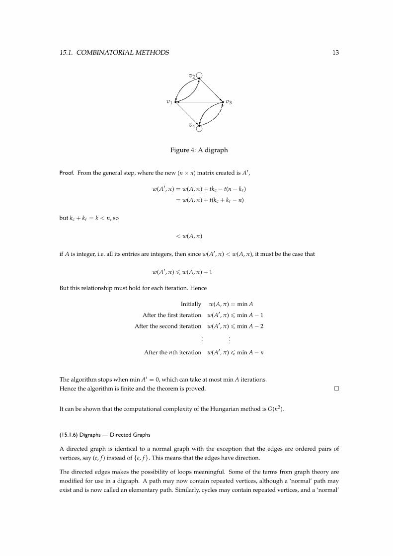
Figure 4: A digraph

Proof. From the general step, where the new (n× n) matrix created is A′,

w(A′, π) = w(A, π) + tkc − t(n− kr)

= w(A, π) + t(kc + kr − n)

but kc + kr = k < n, so

< w(A, π)

if A is integer, i.e. all its entries are integers, then since w(A′, π) < w(A, π), it must be the case that

w(A′, π) 6 w(A, π)− 1

But this relationship must hold for each iteration. Hence

Initially w(A, π) = min A

After the first iteration w(A′, π) 6 min A− 1

After the second iteration w(A′, π) 6 min A− 2

......

After the nth iteration w(A′, π) 6 min A− n

The algorithm stops when min A′ = 0, which can take at most min A iterations.Hence the algorithm is finite and the theorem is proved. �

It can be shown that the computational complexity of the Hungarian method is O(n2).

(15.1.6) Digraphs — Directed Graphs

A directed graph is identical to a normal graph with the exception that the edges are ordered pairs ofvertices, say (e, f ) instead of {e, f }. This means that the edges have direction.

The directed edges makes the possibility of loops meaningful. Some of the terms from graph theory aremodified for use in a digraph. A path may now contain repeated vertices, although a ‘normal’ path mayexist and is now called an elementary path. Similarly, cycles may contain repeated vertices, and a ‘normal’


cycle is called an elementary cycle.

For example, in the digraph in Figure 4, (v1, v2, v2, v3, v4) is a path, and (v4, v3, v1, v2, v3, v1, v4) is a cycle.

For a sizable digraph with a not inconsiderable number of vertices it is clear that the shortest path from onevertex to another is not a trivial matter. Add to this the complexities imposed by a weighting function, andthe problem soon becomes rather unwieldy. For a digraph z = (V, E) with weighting function d : E → R,

the weight of a path P = (v0, v1, . . . , vk) is d(P) =k

∑i=1

d(vi−1, vi). The shortest path problem is to find the

path of minimal weight (or length) between two given vertices.

A solution is found by finding the shortest path from the start vertex s to all other vertices. For a set ofvertices W ⊆ V, define dW (v) to be length of the shortest sv path with all intermediate vertices in W. Thisis the temporary shortest distance. By extending W from {s} to V all the shortest paths can be found andhence solve the problem.

Theorem 38 Choose x ∈ V \W such that dW (x) = min {dW (v) | v ∈ V \W} i.e. the shortest sv path. Let W ′ =W ∪ {x} then for y ∈ V \W, dW ′ (y) = min {dW (y), dW (x) + d(x, y)}

In order to prove this, the following lemma is required

Lemma 39 If x is a vertex selected by the process in Theorem 38, then dW (x) = dV(x).

Proof. Proof Of Lemma 39 A temporary shortest distance must be greater or equal to the actual shortestdistance, hence dW (x) > dV(x).Suppose that dW (x) > dV(x). Then there exists a path P with d(P) = dV(x) that has at least one intermediatevertex not in W. Let z be the first vertex of P that is not in W, then P can be written as P′ + P′′ where P′ is assz path in W and P′′ is the rest of the path.Hence d(P′) + d(P′′) = d(P) < dW (x). But d(P′′) > 0 so d(P′) < dW (P)Now, x was the vertex (not in W) that had the temporary shortest distance. But z /∈ W and d(P′) < dW (P)where by construction P′ is an sz path with intermediate vertices in W which is shorter.Hence by contradiction the lemma holds. �

Proof. Proof Of Theorem 38 Consider y ∈ V \W. dW (y) and dW (x) + d(x, y) are the lengths of two sy pathswith intermediate vertices in W ′, and so

dW ′ (y) 6 min {dW (y), dW (x) + d(x, y)}

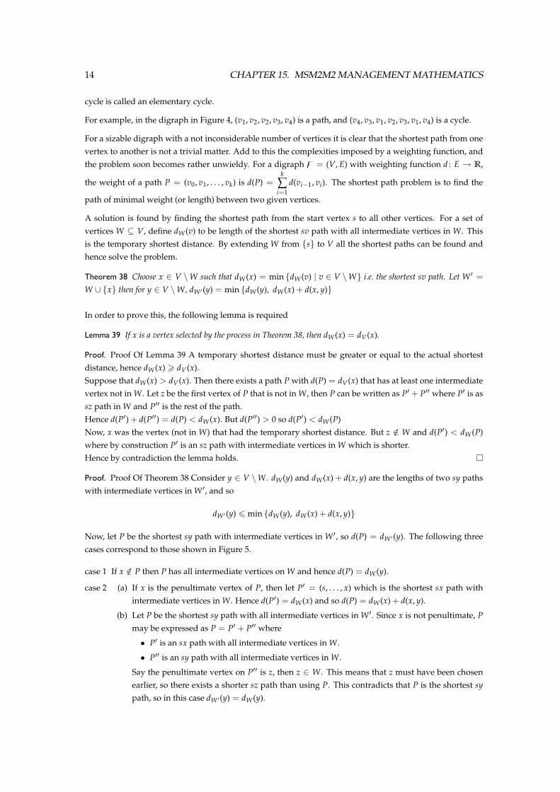
Now, let P be the shortest sy path with intermediate vertices in W ′, so d(P) = dW ′ (y). The following threecases correspond to those shown in Figure 5.

case 1 If x /∈ P then P has all intermediate vertices on W and hence d(P) = dW (y).

case 2 (a) If x is the penultimate vertex of P, then let P′ = (s, . . . , x) which is the shortest sx path withintermediate vertices in W. Hence d(P′) = dW (x) and so d(P) = dW (x) + d(x, y).

(b) Let P be the shortest sy path with all intermediate vertices in W ′. Since x is not penultimate, Pmay be expressed as P = P′ + P′′ where

• P′ is an sx path with all intermediate vertices in W.

• P′′ is an sy path with all intermediate vertices in W.

Say the penultimate vertex on P′′ is z, then z ∈ W. This means that z must have been chosenearlier, so there exists a shorter sz path than using P. This contradicts that P is the shortest sypath, so in this case dW ′ (y) = dW (y).


r r rs s s

r r rx x x

r r ry y yr rz z

W W W

Case 1

��

��*

Case 2(a)

r?

��

Case 2(b)

r�

��*

Figure 5: Pictorial representation of Theorem 38.

In all cases, the shortest sy path is one of dW (y) and dW (x) + d(x, y). Hence

dW ′ (y) = min {dW (y), dW (x) + d(x, y)}

and so the theorem is proved. �

Having shown that this process of finding shortest paths works, it is now possible to formulate the algorithmfor putting this result into practice.

Algorithm 40 Dijkstra For a digraph z = (V, E) and weight function d : E → R the shortest paths from the vertex sare found as follows.

1. (a) Set W := {s}.

(b) Set d(x) := d(s, x) if (s, x) ∈ E else d(x) = ∞.

2. ∀x ∈ V \W find x′ such that dW (x′) = min{dW (x)}.

3. Set W := W ∪ {x′}.

4. For all y ∈ V \W set dW (y) := min{dW (y), dW (x′) + d(x′, y)}.

5. If W = V then stop, else repeat from 2.

Proof. The correctness of the algorithm is shown by Theorem 38.

The computational complexity is calculated for each step in turn.

1. 1 for the assignment, and |V| − 1 = n− 1 for the checking of vertices.

2. Finding x′ can be done in at most |V \W| steps, which is O(n).

3. As assignment and a union, making 2.

4. An addition, a minimum, and an assignment. Each of these must be done for |V \W| vertices, giving3O(n) = O(n).

5. One operation. Note that the loop will be made n− 1 times.

Hence the total computational complexity is

computational complexity = 1 + (n− 1) + (n− 1) (O(n) + 2 + O(n))

6 O(n) + (O(n))2

= O(n) + O(n2)

= O(n2)

Hence the computational complexity is O(n2). �


u u

u u

u u

a

b

c

d

e

f��

��

��

��

5

@@

@@

@@

@R

3

��

��

��

��

��

��

��*

8H

HH

HH

HH

HH

HH

HH

HHj

10

-20

?

8

-9AAAAAAAAAAAAAAU

6

HH

HH

HH

HH

HH

HH

HHHj

10

��

5

-7

��

��

��

��

��

��

��*

10

?

2

@@

@@

@@

@R

4

��

��

��

��

3

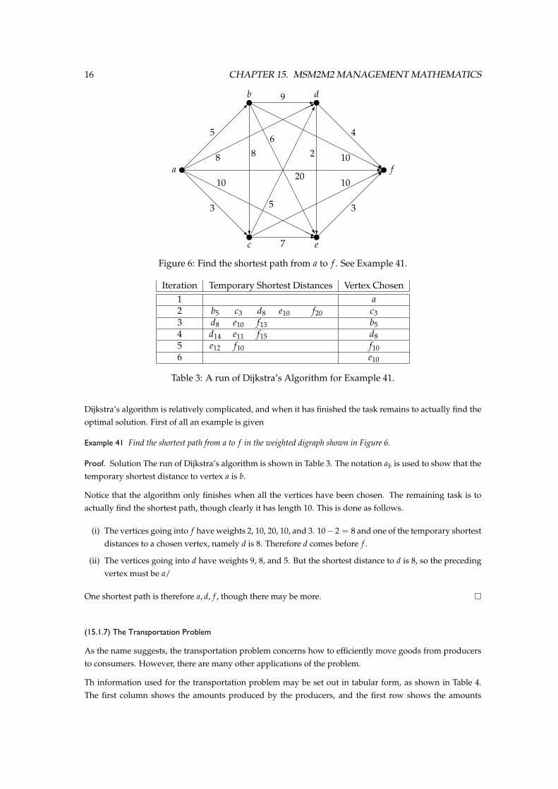
Figure 6: Find the shortest path from a to f . See Example 41.

Iteration Temporary Shortest Distances Vertex Chosen1 a2 b5 c3 d8 e10 f20 c33 d8 e10 f13 b54 d14 e11 f15 d85 e12 f10 f106 e10

Table 3: A run of Dijkstra’s Algorithm for Example 41.

Dijkstra’s algorithm is relatively complicated, and when it has finished the task remains to actually find theoptimal solution. First of all an example is given

Example 41 Find the shortest path from a to f in the weighted digraph shown in Figure 6.

Proof. Solution The run of Dijkstra’s algorithm is shown in Table 3. The notation ab is used to show that thetemporary shortest distance to vertex a is b.

Notice that the algorithm only finishes when all the vertices have been chosen. The remaining task is toactually find the shortest path, though clearly it has length 10. This is done as follows.

(i) The vertices going into f have weights 2, 10, 20, 10, and 3. 10− 2 = 8 and one of the temporary shortestdistances to a chosen vertex, namely d is 8. Therefore d comes before f .

(ii) The vertices going into d have weights 9, 8, and 5. But the shortest distance to d is 8, so the precedingvertex must be a/

One shortest path is therefore a, d, f , though there may be more. �

(15.1.7) The Transportation Problem

As the name suggests, the transportation problem concerns how to efficiently move goods from producersto consumers. However, there are many other applications of the problem.

Th information used for the transportation problem may be set out in tabular form, as shown in Table 4.The first column shows the amounts produced by the producers, and the first row shows the amounts


b1 b2 · · · bn

a1 c11 c12 · · · c1na2 c21 c22 · · · c2n...

......

. . ....

am cm1 cm2 · · · cmn

Table 4: Information for the transportation table.

demanded by the consumers. The central values, cij, show the cost of moving a unit from producer i toconsumer j.

The problem now is to find numbers xij, the amount of goods to be taken from producer i to customerj. The problem can be represented on a bipartite graph—bipartite because taking goods from producer toproducer or consumer to consumer is clearly not an option. Suppose the producers are Ais with productionai and similarly the consumers be Bj with demand bj then clearly the transportation cij is equivalent to theedge {Ai, Bj}.

The objective is to minimise the total cost of transportation, i.e.m

∑i=1

n

∑j=1

xijcij. There are however the obvious

constraints can a producer cannot exceed capacity, and consumers demand as much as is stated and thisdemand must be met.

Model 42 The transportation problem may be formalised as follows. Minimise the quantity f (X) =m

∑i=1

n

∑j=1

xijcij

subject to the constraints

n

∑j=1

xij = ai so supplies must be used (43)

m

∑i=1

xij = bj so demands must be met (44)

xij > 0 for the sake of reality (45)

It is also assumed that supplies and demands are positive i.e. ai > 0 ∀i and bj > 0 ∀j.

f (X) is called the objective function, and X represents the set of xijs of the solution under consideration. Asolution satisfying equations (43), (44), and (45) is called feasible, and when f (X) attains its minimum thesolution is optimal. Note that f (X) does attain its minimum since the set of all possible solutions is finite.Hence if a feasible solution exists, then an optimal solution exists.

Theorem 46 The transportation has a feasible solution if and only ifm

∑i=1

ai =n

∑j=1

bj.

Proof. The theorem has two parts, so each is taken in turn,


⇒ If a solution X is feasible then,

m

∑i=1

ai =m

∑i=1

n

∑j=1

xij by feasibility

=n

∑j=1

m

∑i=1

xij property of sums

=n

∑j=1

bj by feasibility

Hence the ‘only if’ part.

⇐ Suppose thatm

∑i=1

ai =n

∑j=1

bj = t, say.

set xij =aibj

t> 0 so (45) holds

thenn

∑j=1

xij =ait

n

∑j=1

bj = ai so (44) holds

andm

∑i=1

xij =bj

t

m

∑i=1

ai = bj so (43) holds

Furthermore, this proof has revealed a feasible solution to be xij =aibj

t. �

Clearly there is a problem ifm

∑i=1

ai 6=n

∑j=1

bj. In this case a ‘dummy producer’ or a ‘dummy consumer’ can

be introduced with the required capacity or demand. The costs of transportation to these are zero. Hence

without loss of generality it is assumed thatm

∑i=1

ai =n

∑j=1

bj.

The task of finding a feasible solution and in turn an optimal solution is now set about. Note the followingdefinitions.

Definition 47 A solution to the transportation problem is

(i) basic if the associated graph is acyclic.

(ii) degenerate if the associated graph is not connected.

(iii) non-degenerate if the associated graph is a spanning tree.

First of all a basic feasible solution is sought. Note that a degenerate solution can be extended to a non-degenerate one by adding edges of zero weight.

Definition 48 Let X be a basic feasible solution. The base of X is the set B ⊆ (1, 2, . . . m)× (1, 2, . . . n) such that

(i) xij = 0 ∀(i, j) /∈ B.

(ii) The set of vertices{

AiBj | (i, j) ∈ B}

form a spanning tree for the associated graph, Knm.

If a basic feasible solution X is already a spanning tree then the base is unique, but if it is degenerate thenit may be possible to extend to a non-degenerate solution in many ways. A solution can be checked forcycles in the transportation table directly—without having to draw the associated graph. Since the graphis bipartite it is readily deduced that a cycle must join non-zero cells in the table by alternating vertical andhorizontal lines.


Definition 49 The dual solution to the transportation problem is the vector(

α1 α2 . . . αm β1 β2 . . . βn

)where αi + β j = cij∀(i, j) ∈ B.

By fixing βn = 0 the dual solution can be easily found.

Theorem 50 (The Optimality Criterion) Let X be a basic feasible solution, and(

α1 α2 . . . αm β1 β2 . . . βn

)be the dual solution. If αi + β j 6 cij ∀i ∀j then X is an optimal solution.

Proof. Consider some arbitrary feasible solution Y.

f (Y) =m

∑i=1

n

∑j=1

cijyij

>m

∑i=1

n

∑j=1

(αi + β j)yij

=m

∑i=1

n

∑j=1

αiyij +m

∑i=1

n

∑j=1

β jyij

=m

∑i=1

αiai +n

∑j=1

β jbj since Y is feasible

=m

∑i=1

αi

n

∑j=1

xij +n

∑j=1

β j

m

∑i=1

xij since X is feasible

=m

∑i=1

n

∑j=1

(αi + β j)xij

= ∑(i,j)∈B(X)

(αi + β j)xij + ∑(i,j)/∈B(X)

(αi + β j)xij

= ∑(i,j)∈B(X)

cijxij + ∑(i,j)/∈B(X)

(αi + β j)xij

= ∑(i,j)∈B(X)

cijxij since (i, j) /∈ B(X) ⇒ xij = 0

=m

∑i=1

n

∑j=1

cijxij

f (Y) > f (X)

Hence X is an optimal solution since its cost is at most the cost of any other feasible solution. �

Knowing the optimality criterion allows feasible solutions to be checked for being optimal. If they are notthen it is necessary to find a different one and check that. Indeed, a method for finding a single feasiblesolution has not jet been exhibited.

Algorithm 51 (The North-West Corner Rule) The north-west corner rule finds a basic feasible solution as follows

1. Define (r, s) as the top left most ‘available’ cell in the transportation table.

2. Assign xrs := max (ar, bs).

3. Let ar := ar − xrs and make unavailable row r if ar = 0.

4. Let bs := bs − xrs and make unavailable columns s if bs − xrs = 0.

5. If no cell is available the algorithm stops, else repeats from 1.

It is claimed that this process will always find a basic feasible solution.


Proof. By construction the solution is feasible. What remains to be shown is that the solution is basic i.e. theassociated graph is acyclic.Suppose the solution found has a cycle, and let AiBj be the top left most edge of the cycle. There must beedges ArBj and AiBs with non-zero entries in the transportation table in order for a cycle to exist, note r > iand s > j.By hypothesis AiBj is chosen first, and either row i or column j or both are made unavailable. Hence at leastone of ArBj and AiBs cannot also be chosen.Hence by contradiction the theorem is proved. �

Having found a basic feasible solution and found it not to be optimal, a method must now be found tomove to an optimal solution. Since the optimality criterion is violated, ∃i ∃jαi + β j > cij. It is now soughtto include the offending cell in the solution, it will then contribute to the αs and βs and so help get rid of theviolation of the optimality criterion.

By analogy with the associated graph, observe that an edge can be added and one from the resulting cycleremoved leaving another spanning tree. By adding an edge AkBl say, one of the edges ArBl and AkBs mustbe removed, hence let xkl = θ be the minimum of all the xij on the cycle and subtract θ from each of theco-linear and co-columnar edges to AkBl . But then the solution nolonger works, so θ has to be added to thevertices co-linear or co-columnar to those from which θ was subtracted. . . The following algorithm thereforearises

x′ij =

xij − θ if AiBj is an even arc on the cycle

xij + θ if AiBj is an odd arc on the cycle

xij otherwise

Finally, the transportation problem is illustrated by means of a short example.

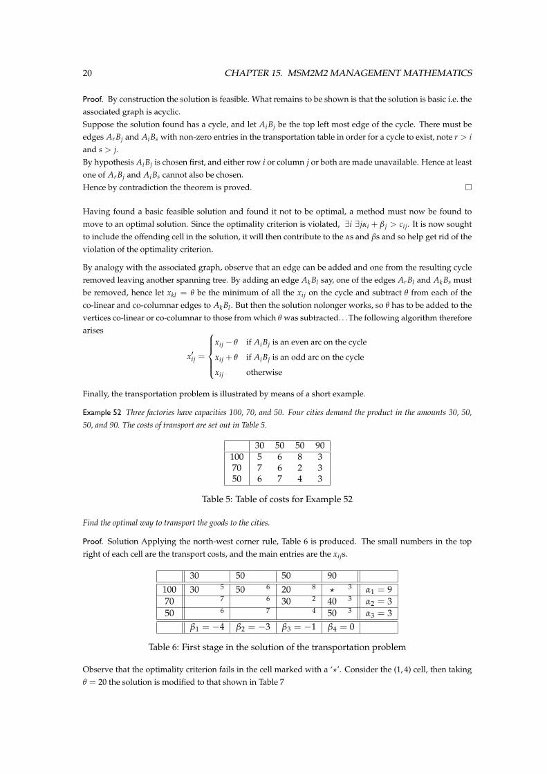
Example 52 Three factories have capacities 100, 70, and 50. Four cities demand the product in the amounts 30, 50,50, and 90. The costs of transport are set out in Table 5.

30 50 50 90100 5 6 8 370 7 6 2 350 6 7 4 3

Table 5: Table of costs for Example 52

Find the optimal way to transport the goods to the cities.

Proof. Solution Applying the north-west corner rule, Table 6 is produced. The small numbers in the topright of each cell are the transport costs, and the main entries are the xijs.

30 50 50 90100 30 5 50 6 20 8 ? 3 α1 = 970 7 6 30 2 40 3 α2 = 350 6 7 4 50 3 α3 = 3

β1 = −4 β2 = −3 β3 = −1 β4 = 0

Table 6: First stage in the solution of the transportation problem

Observe that the optimality criterion fails in the cell marked with a ‘?’. Consider the (1, 4) cell, then takingθ = 20 the solution is modified to that shown in Table 7

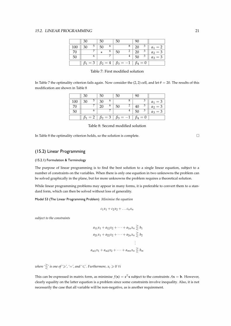
15.2. LINEAR PROGRAMMING 21

30 50 50 90100 30 5 50 6 8 20 3 α1 = 270 7 ? 6 50 2 20 3 α2 = 350 6 7 4 50 3 α3 = 3

β1 = 3 β2 = 4 β3 = −1 β4 = 0

Table 7: First modified solution

In Table 7 the optimality criterion fails again. Now consider the (2, 2) cell, and let θ = 20. The results of thismodification are shown in Table 8

30 50 50 90100 30 5 30 6 8 3 α1 = 370 7 20 6 50 2 40 3 α2 = 350 6 7 4 50 3 α3 = 3

β1 = 2 β2 = 3 β3 = −1 β4 = 0

Table 8: Second modified solution

In Table 8 the optimality criterion holds, so the solution is complete. �

(15.2) Linear Programming

(15.2.1) Formulation & Terminology

The purpose of linear programming is to find the best solution to a single linear equation, subject to anumber of constraints on the variables. When there is only one equation in two unknowns the problem canbe solved graphically in the plane, but for more unknowns the problem requires a theoretical solution.

While linear programming problems may appear in many forms, it is preferable to convert them to a stan-dard form, which can then be solved without loss of generality.

Model 53 (The Linear Programming Problem) Minimise the equation

c1x1 + c2x2 + . . . cnxn

subject to the constraints

a11x1 + a12x2 + · · ·+ a1nxn T b1

a21x1 + a22x2 + · · ·+ a2nxn T b2

...

am1x1 + am2x2 + · · ·+ amnxn T bm

where ‘T’ is one of ‘>’, ‘=’, and ‘6’. Furthermore, xi > 0 ∀i

This can be expressed in matrix form, as minimise f (x) = cTx subject to the constraints Ax = b. However,clearly equality on the latter equation is a problem since some constraints involve inequality. Also, it is notnecessarily the case that all variable will be non-negative, as is another requirement.


To overcome these problems, ‘slack’ variables are introduced. This works as follows,

gi(x) 6 bi ⇔ gi(x) + xn+1 = bi for some xn+1 > 0

gi(x) > bi ⇔ gi(x)− xn+1 = bi for some xn+1 > 0

Similarly, the non-negativity criterion can be solved by re-defining

xk = xn+1 − xn+2 1 6 k 6 n

Having standardised the problem in this way, a number of new variables will have been introduced. It isoften convenient to re-define the subscripts so they run from 1 to some new value of n.

Definition 54 For a linear programming problem in standard form,

1. f (x) = cTx is called the objective function.

2. Every x ∈ Rn satisfying Ax = b and xi > 0 ∀i is called a feasible solution.

3. The set of feasible solutions is denoted by M, and Mopt is the set of all optimal solutions. Hence

Mopt = {x ∈ M | f (x) 6 f (z) ∀z ∈ M}

4. ai is the column vector whose entries are the ith row of the matrix A.

5. Aj is the column vector whose entries are the jth column of the matrix A.

Notice that maximisation can be performed by minimising the negation of the objective function. Recallthat A is an m× n matrix. From the above definitions it is evident that

Ax = b ⇔n

∑j=1

xjAj = b ⇔n

∑j=1

aijxj = bj ∀i ⇔ aTi x = bi ∀i

Finding A Solution

There is nothing to say that Ax = b must have only one solution—if m < n then there are necessarily manysolutions. However, it may be assumed that the rank of A is m since linearly dependent rows could beremoved. From this it follows that there must exist a non-singular m × m submatrix of A, B say. HenceB =

(Aj1 Aj2 . . . Ajm

)for some 1 6 j 6 n−m.

Definition 55 Where B is a non-singular submatrix of A, B =(

Aj1 Aj2 . . . Ajm

)then,

1. The indices j1, j2, . . . , jm are defined by the function B(i) = ji for 1 6 i 6 m.

2. The set B ={

Aj1 , Aj2 , . . . , Ajm

}is called a basis for A, as the vectors span the column space of A.

3. The indices of the basis, i.e. j1, j2, . . . , jm are referred to as ‘basic’.

4. xB =(

xj1 xj2 . . . xjm

)Tis the component of x with basic indices.

5. cB =(

cj1 cj2 . . . cjm

)Tis the component of c with basic indices.

Using this notation, it is evident that

b = Ax =n

∑j=1

Ajxj = ∑A∈B

Ajxj + ∑A/∈B

Ajxj = BxB + ∑A/∈B

Ajxj


Hence a basic solution x satisfies BxB = b and xj = 0 for Aj /∈ B. If also the entries of xB are non-negativethen it is a basic feasible solution, and if xB(i) > 0 then it is non-degenerate. In summary

• A basic feasible solution has zero entries bar for the m entries in the base positions. If any of these mentries are zero, then the basic feasible solution is degenerate.

Having found a solution, its optimality now needs to be assessed.

Theorem 56 (Optimality Criterion) Let zj = cTBB−1Aj and let z =

(z1 z2 . . . zn

)T. If x is a basic feasible

solution and cj − zj > 0∀j then x ∈ Mopt.

Proof. Let y be a feasible solution, so Ay = b and yj > 0∀j.By hypothesis cj − zj > 0∀j, so c− z > 0.Hence (c− z)yT > 0 and so cyT > zyT . This gives

f (y) = cTy > zTy

=n

∑j=1

zjyj

=n

∑j=1

cTBB−1Ajyj

= cTBB−1

n

∑j=1

Ajyj

= cTBB−1b

= cTBxB

= cTx

= f (x)

So f (y) > f (x), and since y was any feasible solution, x must be optimal. �

Note that this optimality criterion is a sufficient but not a necessary condition. It is therefore possible foroptimal solutions to exist which do not obey this criterion.

Corollary 57 If Aj ∈ B then cj − zj = 0.

Proof. By definition, B−1AB(i) = ei, one of the standard ordered basis vectors. Hence

zj = cTBB−1Aj =

(cB(1) cB(2) . . . cB(m)

)ei = cB(i) = cj

Hence the result. �

Finding A Better Solution

Finding a solution and assessing its viability is all very well, but if the solution is not optimal then anothersolution must be found and tried. Ideally a new solution will be better than the old one in that the value ofthe objective function will be nearer its minimum.

From this point it will be necessary to distinguish between bases, and so the notation B1,B2, . . . will beused. In the case of the first basis,

BxB1 =m

∑i=1

AB1(i)xB1(i) = b (58)


where AB1(i) represents the ith column of B.

The matrix B−1 A has an important role, so for convenience its columns will be denoted by A′j =

(a′1j a′2j . . . a′mj

)T.

Hence A′ = B−1 A ⇔ A = BA′ gives

BA′j = Aj ⇔

n

∑i=1

AB1(i)a′ij = Aj

where AB1(i) represents the ith column of B. This matrix will become A in the next iteration.

Now, since this is leading to finding another solution, it is assumed that the optimality criterion has beenviolated. Say this is so for column l, so cl − zl < 0, 1 6 l 6 n. In particular the above now gives

n

∑i=1

AB1(i)a′il = Al (59)

Now consider a parameter θ, and find the difference between the solution as it stands, and θ times theoffending column i.e. (58)−θ(59) giving

θAl +m

∑i=1

AB1(i)(

xB1(i) − θa′il)

= b

The expression on the left hand side represents a new solution, with the existing basic solutions beingadjusted, another (l) being added, and the others remaining zero. The new solution is given by

x′ =

xB1(i) 7→ xB1(i) − θa′il 1 6 i 6 m

xl 7→ θ

xj 7→ 0 j 6= l Aj /∈ B

(60)

However, this isn’t a new solution yet: a value for θ has to be found.

If θ = 0 then x′ = x, the old solution†. In order to maintain feasibility, it is clear that θ > 0, so start from 0and increase to make θ as big as possible. The point when θ will be maximal is determined by the top lineof (60) when for some k, xB1(k) − θa′kl = 0. Hence

θ =xB1(k)

a′kl= min

(xB1(i)

a′il| 1 6 i 6 m a′il > 0

)Notice that since xB1(k) − θa′kl = 0, the vector Ak drops out of the basis and is replaced by Al . However, aproblem still remains: in order for B−1 to exist the new basis vectors must be linearly independent, since itis used to define x′.

Theorem 61 The new basis, B2 =(B \

{AB(k)

})∪{

AB(l)}

is linearly independent.

It can be shown that cTx′ = cTx + θ(cl − zl) from which it is obvious that the value of the objective functionhas been reduced. A new and better basic feasible solution has now been found, but there remain two issuesto be addressed.

Firstly, if θ = 0 then x does not change. The fact that θ = 0 at all means that x was degenerate. However, thebasis is still changed by “replacing one zero by another”.

†It would be more correct to say ‘basic feasible solution’ rather than just ‘solution’.


Secondly, there is a problem if a′il 6 0 ∀i. In this case θ → −∞ and this gives

cTx′ = cTx + θ(cl − zl) → −∞

negative because column l violates the optimality criterion. It may be possible to choose some sufficientlylarge value of θ so that the objective function has smaller value. On the other hand the linear programmingproblem may have no solution.

Solving The Linear Programming Problem

At this point enough theory has been covered to actually solve a linear programming problem. This theorycan be neatly packaged into the ‘Simplex Method’. However, it is necessary to make a few assumptions,which will be eliminated in the following section.

Given a linear programming problem in the standard form

f (x) = cTx → min Ax = b xj > 0 ∀j

assume that A contains the m × m identity matrix as a submatrix, and bj > 0 ∀j. These assumptions mayseem trivial to achieve, but meeting both conditions at the same time is rather more difficult than meetingjust one of them.

The value of the assumption is that B = I so that A′j = B−1Aj = Aj. Also, xB = b. The identity matrix in A

is there because of the slack variables. If Ax > b or Ax < b then one slack variable must be added for eachof the m constraints. This produces a constraint equation of the form Ax + Iw = b. These slack variablesmake no appearance in the objective function, so it follows that cB(i) = 0 ∀i. This means that z = 0 so forthe basis subscripts, the relative costs must be 0.The assorted information is usually displayed in a ‘SimplexTable’ as shown in Table 15.2.1.

0 c1 c2 . . . cB(1) . . . cB(m) . . . cn

−z0 c1 − z1 c2 − z2 . . . 0 . . . 0 . . . cn − zncB(1)

... xB A′1 A′

2 . . . identity matrix . . . A′n

cB(m)

Table 9: General form of a ‘Simplex Table’.Note that it is usual to omit the first row and first column. Note also that the quantity −z0 iscalculated as c0 − z0 = 0− cT

Bx, this is the same as f (x).

From the Simplex Table it is a trivial matter to check the optimality criterion, and whether there is in fact nosolution. Assuming the optimality criterion fails but there is a solution, a new solution can be constructedusing the methods described above. But there is a better way.

In the equation BA′ = A, B is the matrix whose columns are the vectors of the basis. The columns of A′ aretherefore the coefficients which produce the corresponding columns of A from the basis vectors. In order tokeep the standard form of the Simplex table, Al , the vector replacing Ak in the basis is required be the kthstandard basis vector. The basis therefore needs to be transformed. Recall that

θ =xB(k)

a′kl= min

(xia′il

| 1 6 i 6 m)

and the chosen xkl is called the pivot. In order to transform the basis,


• divide row k by the pivot.

• subtract from each row that row’s entry (xil) times row k for i 6= l.

This is really just Gaussian elimination, and results in the formula

a′′ij =

a′kja′kl

i = k

a′ij − a′ila′kja′kl

i 6= k(62)

While this is all very well for the main body of the table, there is still the matter of xB and the adjusted costs(and z0). Now, if x is any feasible solution,

f (x) = ∑Aj /∈B

cjxj +m

∑i=1

cB(i)xB(i) = ∑Aj /∈B

cjxj + cTBxB (63)

and every feasible solution also satisfies

b = BxB + ∑Aj /∈B

Ajxj

so B−1b = xB + ∑Aj /∈B

B−1Ajxj

and cTBB−1b = cT

BxB + ∑Aj /∈B

cTBB−1Ajxj

i.e. z0 = cTBxB + ∑

Aj /∈Bzjxj (64)

Comparing equations (63) and (64) it is evident that

f (x)− z0 = ∑Aj /∈B

(cj − zj)xj

z0 = ∑Aj /∈B

(cj − zj)xj − ∑Aj /∈B

cjxj − cTBxB

= − ∑Aj /∈B

zjxj − cTBxB but xj = 0 for j /∈ B, so

= −cTBxB

But this is the definition of z0, so this method also works in the first row of the Simplex table. This ratherconfusing notation becomes rather more transparent in the following example.

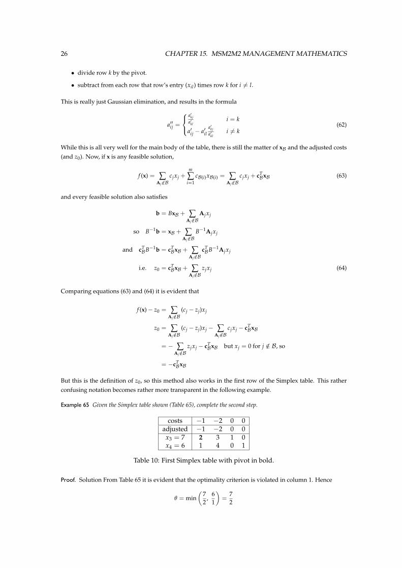
Example 65 Given the Simplex table shown (Table 65), complete the second step.

costs −1 −2 0 0adjusted −1 −2 0 0x3 = 7 2 3 1 0x4 = 6 1 4 0 1

Table 10: First Simplex table with pivot in bold.

Proof. Solution From Table 65 it is evident that the optimality criterion is violated in column 1. Hence

θ = min(

72

,61

)=

72


so it is x3 that is eliminated in favour of x1.Here k is the first row of x3 and l is the first column. For example in the second column,

• from the first case in (62),

a′′12 =32

• from the second case in (62),

c2 − z2 = −2− (− 1)32

=−12

and a′′22 = 4− 132

=52

This can be continued for the other 2 columns. The ‘zero-th’ column is treat in the same way. The twoentries are

x1 = θ =72

and x4 = 6− 172

=52

The new Simplex table is therefore as shown in Table 24

costs −1 −2 0 0adjusted 0 −1

212 0

x2 = 72 1 3

212 0

x4 = 52 0 5

2−12 1

�

Table 11: Second Simplex table.

So it is now possible to solve a standard linear programming problem. However, a number of issues arise.

• In moving from one basis to another, will an already used basis be returned to—will the solutioncycle? This is only an issue if the solutions are degenerate, since otherwise the objective functionalways decreases.

• Anti-cycling rules exist, and if used the method must terminate since there are finitely many bases —(nm

)to be precise. From this finiteness it follows that either the linear programming problem has a

solution, or f → −∞.

• If there are two columns violating the optimality criterion which one should be chosen? As it happens,random choice is as good a strategy as any.

• How complex is the simplex method? Each pivoting requires a polynomial number of operations, but

the number of bases is(

nm

). There are rare cases that can be solved in ‘time’ which is a polynomial

in m and n, but generally this is not so.

• Does a method of polynomial order for solving the linear programming problem exist?

Transformation To Standard Form

For the Simplex method to work it is required that A has as a submatrix the m × m identity matrix, andbi > 0 ∀i. Satisfying the latter condition is simply a case of negating the offending equation, so this on itsown can be assumed without loss of generality. The problem now is to include the former criterion at thesame time.

In transforming any given problem into standard form it is necessary to introduce at most one slack variablefor each constraint equation, but some of them may be negative, so this does not really work. Once theproblem is in standard form, add one slack variable to each auxiliary equation, the problem then has theform Ax + Iw = b.


However, economies can be made since if A already has some identity matrix columns, k say, then onlym− k extra slack variables need be added (and possibly variable re-numbered). Also in the case Ax = b theslack variables added to produce standard from will provide some identity matrix columns.

The auxiliary problem is to minimisem

∑i=1

wi i.e.

(0 0 . . . 0 1 1 . . . 1

)( xw

)→ min

(A I

)( xw

)= b

(xw

)> 0

Since

(xw

)=

(0b

)is always a basic feasible solution which has objective function bounded below by 0,

the Simplex method must terminate after a finite number of steps. Clearly this problem can be solved usingthe Simplex method, and there are two main conclusions.

1. If there are no wis in the solution, so w = 0 then the columns in the Simplex table for w can beremoved and the resulting ‘A’ matrix has an identity submatrix. The Simplex method can now beused on this problem.

2. If it is not possible to eliminate some of the wis then the problem is infeasible and cannot be solved.This is because from the definition of the auxiliary problem the optimal solutions have objective func-tion value of zero. A non-zero wi contradicts this.

The problem just solved has cost co-efficients(

0 0 . . . 0 1 1 . . . 1)

which is clearly not the orig-inal problem. Assuming w = 0 the original problem is solved by deleting the columns of the auxiliarysimplex table corresponding to w. However, it is necessary to re-calculate the row of adjusted costs usingthe original cost coefficients. The following technique is used, and is known as the two-phase method.

1. Transform the problem into standard form.

2. Add one slack variable, wi, to each constraint equation.

3. Use the simplex method to solve the auxiliary problem, this produces the required identity submatrix.

4. Use the simplex method to solve the original problem.

The two-phase method and simplex method are actually a way to solve simultaneous linear inequalities:Linear programming is simply one particular application of it.

(15.2.2) Dual Solution To Linear Programming

Formulating The Dual Solution

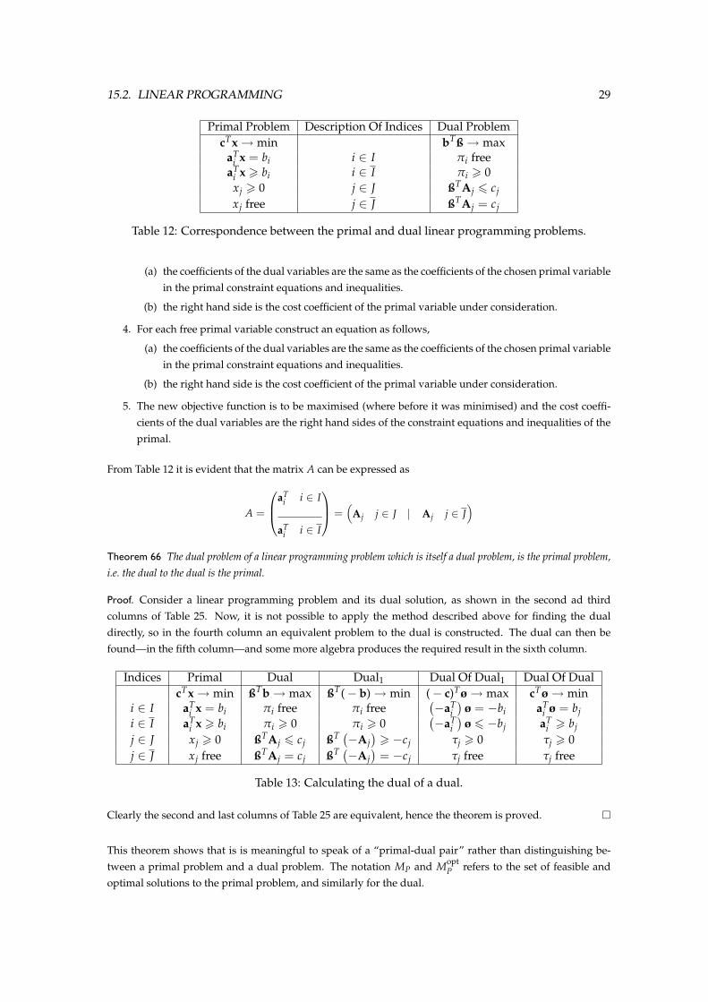
The dual linear programming problem to a given linear programming problem is constructed as shown inTable 12.

The method for converting from the primal to the dual is, therefore,

1. For every equation in the primal there is a free variable in the dual.

2. For every inequality in the primal there is a restricted variable in the dual.

3. For each restricted primal variable construct an inequality with reversed sense (i.e. ‘6’ instead of ‘>’)as follows,


Primal Problem Description Of Indices Dual ProblemcTx → min bTß → max

aTi x = bi i ∈ I πi free

aTi x > bi i ∈ I πi > 0xj > 0 j ∈ J ßTAj 6 cjxj free j ∈ J ßTAj = cj

Table 12: Correspondence between the primal and dual linear programming problems.

(a) the coefficients of the dual variables are the same as the coefficients of the chosen primal variablein the primal constraint equations and inequalities.

(b) the right hand side is the cost coefficient of the primal variable under consideration.

4. For each free primal variable construct an equation as follows,

(a) the coefficients of the dual variables are the same as the coefficients of the chosen primal variablein the primal constraint equations and inequalities.

(b) the right hand side is the cost coefficient of the primal variable under consideration.

5. The new objective function is to be maximised (where before it was minimised) and the cost coeffi-cients of the dual variables are the right hand sides of the constraint equations and inequalities of theprimal.

From Table 12 it is evident that the matrix A can be expressed as

A =

aTi i ∈ I

aTi i ∈ I

=(

Aj j ∈ J | Aj j ∈ J)

Theorem 66 The dual problem of a linear programming problem which is itself a dual problem, is the primal problem,i.e. the dual to the dual is the primal.

Proof. Consider a linear programming problem and its dual solution, as shown in the second ad thirdcolumns of Table 25. Now, it is not possible to apply the method described above for finding the dualdirectly, so in the fourth column an equivalent problem to the dual is constructed. The dual can then befound—in the fifth column—and some more algebra produces the required result in the sixth column.

Indices Primal Dual Dual1 Dual Of Dual1 Dual Of DualcTx → min ßTb → max ßT(− b) → min (− c)Tø → max cTø → min

i ∈ I aTi x = bi πi free πi free

(−aT

i)

ø = −bi aTi ø = bj

i ∈ I aTi x > bi πi > 0 πi > 0

(−aT

i)

ø 6 −bj aTi > bj

j ∈ J xj > 0 ßTAj 6 cj ßT (−Aj)

> −cj τj > 0 τj > 0j ∈ J xj free ßTAj = cj ßT (−Aj

)= −cj τj free τj free

Table 13: Calculating the dual of a dual.

Clearly the second and last columns of Table 25 are equivalent, hence the theorem is proved. �

This theorem shows that is is meaningful to speak of a “primal-dual pair” rather than distinguishing be-tween a primal problem and a dual problem. The notation MP and Mopt

P refers to the set of feasible andoptimal solutions to the primal problem, and similarly for the dual.


Information Provided By The Dual

Theorem 67 (Weak Duality Theorem) ∀x ∈ MP ∀ß ∈ MD cTx > ßTB i.e. for all feasible solutions, f (x) >

φ(ß).

Proof. Now, specifically for j ∈ J, cj > ßTAj. However, when j ∈ J there is equality, so the relationshipholds in general. Similarly bi 6 aT

i x. Hence,

f (x) = cTx = ∑j

cjxj φ(ß) = ßTb = ∑i

πibi

> ∑j

ßTAjxj 6 ∑i

πiaTi x

= ßT Ax = ßT Ax �

From this result it is readily seen that

1. If x ∈ MP, if ß ∈ MD, and if f (x) = φ(ß) then x ∈ MoptP and ß ∈ Mopt

D .

2. (a) If minx∈MP

f (x) = −∞ then MD = ∅.

(b) If maxß∈MD

φ(ß) = ∞ then MP = ∅.

Theorem 68 (Strong Duality Theorem) MoptP 6= ∅ ⇔ Mopt

D 6= ∅ and when this is so, minx∈MP

f (x) = maxß∈MD

φ(ß).

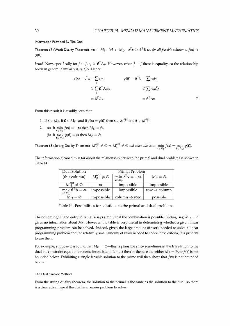
The information gleaned thus far about the relationship between the primal and dual problems is shown inTable 14.

Dual Solution Primal Problem(this column) Mopt

P 6= ∅ minx∈MP

cTx = −∞ MP = ∅

MoptD 6= ∅ ⇔ impossible impossible

maxß∈MD

ßTb = ∞ impossible impossible row ⇒ column

MD = ∅ impossible column ⇒ row possible

Table 14: Possibilities for solutions to the primal and dual problems.

The bottom right hand entry in Table 14 says simply that the combination is possible: finding, say, MD = ∅gives no information about MP. However, the table is very useful in determining whether a given linearprogramming problem can be solved. Indeed, given the large amount of work needed to solve a linearprogramming problem and the relatively small amount of work needed to check these criteria, it is prudentto use them.

For example, suppose it is found that MD = ∅—this is plausible since sometimes in the translation to thedual the constraint equations become inconsistent. It must then be the case that either MP = ∅, or f (x) is notbounded below. Exhibiting a single feasible solution to the prime will then show that f (x) is not boundedbelow.

The Dual Simplex Method

From the strong duality theorem, the solution to the primal is the same as the solution to the dual, so thereis a clear advantage if the dual is an easier problem to solve.

15.3. GAME THEORY 31

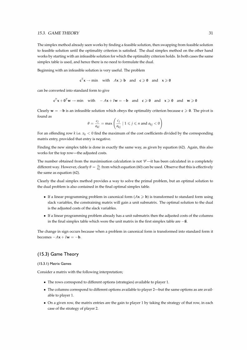
The simplex method already seen works by finding a feasible solution, then swapping from feasible solutionto feasible solution until the optimality criterion is satisfied. The dual simplex method on the other handworks by starting with an infeasible solution for which the optimality criterion holds. In both cases the samesimplex table is used, and hence there is no need to formulate the dual.

Beginning with an infeasible solution is very useful. The problem

cTx → min with Ax > b and c > 0 and x > 0

can be converted into standard form to give

cTx + 0Tw → min with − Ax + Iw = −b and c > 0 and x > 0 and w > 0

Clearly w = −b is an infeasible solution which obeys the optimality criterion because c > 0. The pivot isfound as

θ =clakl

= max

(cj

akj| 1 6 j 6 n and akj < 0

)For an offending row k i.e. xk < 0 find the maximum of the cost coefficients divided by the correspondingmatrix entry, provided that entry is negative.

Finding the new simplex table is done in exactly the same way, as given by equation (62). Again, this alsoworks for the top row—the adjusted costs.

The number obtained from the maximisation calculation is not ‘θ’—it has been calculated in a completelydifferent way. However, clearly θ = xk

aklfrom which equation (60) can be used. Observe that this is effectively

the same as equation (62).

Clearly the dual simplex method provides a way to solve the primal problem, but an optimal solution tothe dual problem is also contained in the final optimal simplex table.

• If a linear programming problem in canonical form (Ax > b) is transformed to standard form usingslack variables, the constraining matrix will gain a unit submatrix. The optimal solution to the dualis the adjusted costs of the slack variables.

• If a linear programming problem already has a unit submatrix then the adjusted costs of the columnsin the final simplex table which were the unit matrix in the first simplex table are −ß.

The change in sign occurs because when a problem in canonical form is transformed into standard form itbecomes −Ax + Iw = −b.

(15.3) Game Theory

(15.3.1) Matrix Games

Consider a matrix with the following interpretation;

• The rows correspond to different options (strategies) available to player 1.

• The columns correspond to different options available to player 2—but the same options as are avail-able to player 1.

• On a given row, the matrix entries are the gain to player 1 by taking the strategy of that row, in eachcase of the strategy of player 2.


• On a given column each matrix entry represents the gain to player 1 if player 2 takes the strategy ofthat column.

Clearly the objective of player 1 is to maximise the minimum gain it can guarantee by choosing the maxi-mum of the row minima.Player 2 on the other hand wishes to minimise the gain of player 1 by choosing the strategy which minimisesthe column maxima.

It is assumed that whatever strategy is finally taken, the gain to player 1 and to player 2 is a constant sum—zero when the game is in standard form. It is also assumed that each player knows what the matrix—thepayoff matrix–is, and that they could make the best decision for themselves if they know what the otherplayer was going to do.

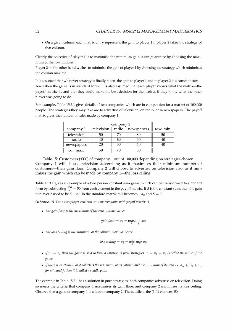
For example, Table 15.3.1 gives details of two companies which are in competition for a market of 100,000people. The strategies they may take are to advertise of television, on radio, or in newspapers. The payoffmatrix gives the number of sales made by company 1.

company 2company 1 television radio newspapers row. min.television 50 70 80 50

radio 40 60 50 40newspapers 20 30 40 40

col. max. 50 70 80

Table 15: Customers (’000) of company 1 out of 100,000 depending on strategies chosen.Company 1 will choose television advertising as it maximises their minimum number ofcustomers—their gain floor. Company 2 will choose to advertise on television also, as it min-imises the gain which can be made by company 1—the loss ceiling.

Table 15.3.1 gives an example of a two person constant sum game, which can be transformed to standardform by subtracting 100

2 = 50 from each element in the payoff matrix. If S is the constant sum, then the gainto player 2 used to be S− aij. In the standard matrix this becomes −aij and S = 0.

Definition 69 For a two player constant sum matrix game with payoff matrix A,

• The gain floor is the maximum of the row minima, hence

gain floor = v1 = maxi

minj

aij

• The loss ceiling is the minimum of the column maxima, hence

loss ceiling = v2 = minj

maxi

aij

• If v1 = v2 then the game is said to have a solution is pure strategies. v = v1 = v2 is called the value of thegame.

• If there is an element of A which is the maximum of its column and the minimum of its row, i.e. ais 6 ars 6 arj

for all i and j, then it is called a saddle point.

The example in Table 15.3.1 has a solution in pure strategies: both companies advertise on television. Doingso meets the criteria that company 1 maximises its gain floor, and company 2 minimises its loss ceiling.Observe that a gain to company 1 is a loss to company 2. The saddle is the (1, 1) element, 50.

15.3. GAME THEORY 33

Theorem 70 v1 6 v2.

Proof.

minj

aij 6 ais for all i and any s chosen

so maxi

minj

aij 6 maxi

ais for any s

v1 6 maxi

ais for any s

v1 6 mins

maxi

ais = v2 �

Theorem 71 If ars is a saddle point, then v1 = ars = v2.

Proof.

v2 = minj

maxi

aij 6 maxi

ais = ars = minj

arj 6 maxi

minj

aij = v1 6 v2

This rather involved series of inequalities proves the theorem. �

Theorem 72 If ars and akl are saddle points, then so are arl and aks.

Proof. Since akl is its row minimum and ars is its column maximum,

akl 6 aks 6 ars

But ars = akl , hence the result. �

If v1 = v2 = v it does not follow that any element of A which is equal to v is a saddle point—it must also beits row minimum and column maximum.

Theorem 73 If v1 = v2 = v then a saddle point exists, and for every saddle point apq, apq = v.

Proof.

Say that v1 = maxi

minj

aij = minj

akj = akl

and v2 = minj

maxi

aij = maxi

ais = ars

This givesaks > akl = v and aks 6 ars = v

So it must be the case that aks = akl = ars and hence

aks = minj

akj = maxi

ais

i.e. aks is a saddle point. �

(15.3.2) Solution In Mixed Strategies

It is quite possible that the maximum of the row minima, and the minimum of the column maxima do notcoincide i.e. there is no saddle point. In this case there is no sure-fire strategy for either of the players.


Definition 74 The mixed strategy of player 1 is the probability distribution on the set of pure strategies which yield—inthe long term—the maximum profit.

Instead of picking the same strategy each time, the players will now choose different strategies, and it isnecessary to calculate the frequency with which they choose the various strategies. Say

• Player 1 chooses strategy i with probability xi.

• Player 2 chooses strategy j with probability yj.

This means that any particular combination will occur is xiyj. These are independent events because player1 does not know in advance how player 2 will play, and vice versa. The expected gain for player 1 is then

m

∑i=1

n

∑j=1

aijxiyj = xT Ay

Define Sk =

{(z1, z2, . . . , zk) | zi > 0 ∀i and

k

∑i=1

zi = 1

}so that

v1 = maxx∈Sm

miny∈Sn

xT Ay the gain floor

v2 = miny∈Sn

maxx∈Sm

xT Ay the loss ceiling

As with solutions in pure strategies, v1 6 v2, and in fact v1 = v2 for all matrices. A solution (x∗, y∗) ∈Sm × Sn must satisfy

miny∈Sn

(x∗)T Ay = v1 = v2 = maxx∈Sm

xT A (y∗)T

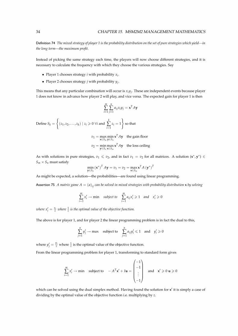
As might be expected, a solution—the probabilities—are found using linear programming.

Assertion 75 A matrix game A = (a)ij can be solved in mixed strategies with probability distribution x by solving

m

∑i=1

x′i → min subject tom

∑i=1

aijx′i > 1 and x′i > 0

where x′i = xiz where 1

z is the optimal value of the objective function.

The above is for player 1, and for player 2 the linear programming problem is in fact the dual to this,

n

∑j=1

y′j → max subject ton

∑j=1

aijy′i 6 1 and y′i > 0

where y′j = yjz where 1

z is the optimal value of the objective function.

From the linear programming problem for player 1, transforming to standard form gives

m

∑i=1

x′i → min subject to − ATx′ + Iu =

−1−1

...−1

and x′ > 0 u > 0

which can be solved using the dual simplex method. Having found the solution for x′ it is simply a case ofdividing by the optimal value of the objective function i.e. multiplying by z.

Documents

Chapter 15 MSM2M2 Introduction To Management …igor.gold.ac.uk/~mas01rwb/notes/2M2.pdfMSM2M2 Introduction To Management Mathematics ... a simpliﬁed form of it — its ‘O’ set