Embed Size (px)
Citation preview
Chapter 14 Turbomachinery
14-1 PROPRIETARY MATERIAL. © 2014 by McGraw-Hill Education. This is proprietary material solely for authorized instructor use. Not authorized for sale or distribution in any manner. This document may not be copied, scanned, duplicated, forwarded, distributed, or posted on a website, in whole or part.
Solutions Manual for
Fluid Mechanics: Fundamentals and Applications Third Edition
Yunus A. Çengel & John M. Cimbala
McGraw-Hill, 2013
Chapter 14 TURBOMACHINERY
PROPRIETARY AND CONFIDENTIAL This Manual is the proprietary property of The McGraw-Hill Companies, Inc. (“McGraw-Hill”) and protected by copyright and other state and federal laws. By opening and using this Manual the user agrees to the following restrictions, and if the recipient does not agree to these restrictions, the Manual should be promptly returned unopened to McGraw-Hill: This Manual is being provided only to authorized professors and instructors for use in preparing for the classes using the affiliated textbook. No other use or distribution of this Manual is permitted. This Manual may not be sold and may not be distributed to or used by any student or other third party. No part of this Manual may be reproduced, displayed or distributed in any form or by any means, electronic or otherwise, without the prior written permission of McGraw-Hill.

Chapter 14 Turbomachinery
14-2 PROPRIETARY MATERIAL. © 2014 by McGraw-Hill Education. This is proprietary material solely for authorized instructor use. Not authorized for sale or distribution in any manner. This document may not be copied, scanned, duplicated, forwarded, distributed, or posted on a website, in whole or part.
General Problems 14-1C Solution We are to list examples of fans, blowers, and compressors. Analysis Common examples of fans are window fans, ceiling fans, fans in computers and other electronics equipment, radiator fans in cars, etc. Common examples of blowers are leaf blowers, hair dryers, air blowers in furnaces and automobile ventilation systems. Common examples of compressors are tire pumps, refrigerator and air conditioner compressors. Discussion Students should come up with a diverse variety of examples.
14-2C Solution We are to discuss the differences between fans, blowers, and compressors. Analysis A fan is a gas pump with relatively low pressure rise and high flow rate. A blower is a gas pump with relatively moderate to high pressure rise and moderate to high flow rate. A compressor is a gas pump designed to deliver a very high pressure rise, typically at low to moderate flow rates. Discussion The boundaries between these three types of pump are not always clearly defined.
14-3C Solution We are to discuss energy producing and energy absorbing devices. Analysis A more common term for an energy producing turbomachine is a turbine. Turbines extract energy from the moving fluid, and convert that energy into useful mechanical energy in the surroundings, usually in the form of a rotating shaft. Thus, the phrase “energy producing” is from a frame of reference of the fluid – the fluid loses energy as it drives the turbine, producing energy to the surroundings. On the other hand, a more common term for an energy absorbing turbomachine is a pump. Pumps absorb mechanical energy from the surroundings, usually in the form of a rotating shaft, and increase the energy of the moving fluid. Thus, the phrase “energy absorbing” is from a frame of reference of the fluid – the fluid gains or absorbs energy as it flows through the pump. Discussion From the frame of reference of the surroundings, a pump absorbs energy from the surroundings, while a turbine produces energy to the surroundings. Thus, you may argue that the terminology also holds for the frame of reference of the surroundings. This alternative explanation is also acceptable.
14-4C Solution We are to discuss the difference between a positive-displacement turbomachine and a dynamic turbomachine. Analysis A positive-displacement turbomachine is a device that contains a closed volume; energy is transferred to the fluid (pump) or from the fluid (turbine) via movement of the boundaries of the closed volume. On the other hand, a dynamic turbomachine has no closed volume; instead, energy is transferred to the fluid (pump) or from the fluid (turbine) via rotating blades. Examples of positive-displacement pumps include well pumps, hearts, some aquarium pumps, and pumps designed to release precise volumes of medicine. Examples of positive-displacement turbines include water meters and gas meters in the home. Examples of dynamic pumps include fans, centrifugal blowers, airplane propellers, centrifugal water pumps (like in a car engine), etc. Examples of dynamic turbines include windmills, wind turbines, turbine flow meters, etc. Discussion Students should come up with a diverse variety of examples.
Chapter 14 Turbomachinery
14-3 PROPRIETARY MATERIAL. © 2014 by McGraw-Hill Education. This is proprietary material solely for authorized instructor use. Not authorized for sale or distribution in any manner. This document may not be copied, scanned, duplicated, forwarded, distributed, or posted on a website, in whole or part.
14-5C Solution We are to explain the “extra” term in the Bernoulli equation in a rotating reference frame. Analysis A rotating reference frame is not an inertial reference frame. When we move outward in the radial direction, the absolute velocity at this location is faster due to the rotating body, since v is equal to r. When solving a turbomachinery problem in a rotating reference frame, we use the relative fluid velocity (velocity relative to the rotating reference frame). Thus, in order for the Bernoulli equation to be physically correct, we must subtract the absolute velocity of the rotating body so that the equation applies to an inertial reference frame. This accounts for the “extra” term. Discussion The Bernoulli equation is the same physical equation in either the absolute or the rotating reference frame, but it is more convenient to use the form with the extra term in turbomachinery applications.
14-6C Solution We are to discuss the difference between brake horsepower and water horsepower, and then discuss turbine efficiency. Analysis In turbomachinery terminology, brake horsepower is the power actually delivered by the turbine to the shaft. (One may also call it “shaft power”.) On the other hand, water horsepower is the power extracted from the water flowing through the turbine. Water horsepower is always greater than brake horsepower; because of inefficiencies; hence turbine efficiency is defined as the ratio of brake horsepower to water horsepower. Discussion For a pump, efficiency is defined in the opposite way, since brake horsepower is greater than water horsepower.
14-7C Solution We are to discuss the difference between brake horsepower and water horsepower, and then discuss pump efficiency. Analysis In turbomachinery terminology, brake horsepower is the power actually delivered to the pump through the shaft. (One may also call it “shaft power”.) On the other hand, water horsepower is the useful portion of the brake horsepower that is actually delivered to the fluid. Water horsepower is always less than brake horsepower; hence pump efficiency is defined as the ratio of water horsepower to brake horsepower. Discussion For a turbine, efficiency is defined in the opposite way, since brake horsepower is less than water horsepower.

Chapter 14 Turbomachinery
14-4 PROPRIETARY MATERIAL. © 2014 by McGraw-Hill Education. This is proprietary material solely for authorized instructor use. Not authorized for sale or distribution in any manner. This document may not be copied, scanned, duplicated, forwarded, distributed, or posted on a website, in whole or part.
14-8 Solution For an air compressor with equal inlet and outlet areas, and with both density and pressure increasing, we are to determine how the average speed at the outlet compares to the average speed at the inlet. Assumptions 1 The flow is steady. Analysis Conservation of mass requires that the mass flow rate in equals the mass flow rate out. The cross-sectional areas of the inlet and outlet are the same. Thus,
Conservation of mass: in in in in out out out outm V A m V A & &
or
inout in
out
V V
(1)
Since in < out, Vout must be less than Vin. Discussion A compressor does not necessarily increase the speed of the fluid passing through it. In fact, the average speed through the pump can actually decrease, as it does here.
14-9 Solution We are to determine how the average speed at the outlet compares to the average speed at the inlet of a water pump. Assumptions 1 The flow is steady (in the mean). 2 The water is incompressible. Analysis Conservation of mass requires that the mass flow rate in equals the mass flow rate out. Thus,
Conservation of mass: in in in in out out out outm V A m V A & &
or, since the cross-sectional area is proportional to the square of diameter,
2 2
in in inout in in
out out out
D DV V V
D D
(1)
(a) For the case where Dout < Din, Vout must be greater than Vin.
(b) For the case where Dout = Din, Vout must be equal to Vin.
(c) For the case where Dout > Din, Vout must be less than Vin. Discussion A pump does not necessarily increase the speed of the fluid passing through it. In fact, the average speed through the pump can actually decrease, as it does here in part (c).

Chapter 14 Turbomachinery
14-5 PROPRIETARY MATERIAL. © 2014 by McGraw-Hill Education. This is proprietary material solely for authorized instructor use. Not authorized for sale or distribution in any manner. This document may not be copied, scanned, duplicated, forwarded, distributed, or posted on a website, in whole or part.
Pumps
14-10C Solution We are to define and discuss NPSH and NPSHrequired. Analysis Net positive suction head (NPSH) is defined as the difference between the pump’s inlet stagnation pressure head and the vapor pressure head,
2
pump inlet
NPSH2
vPP Vg g g
We may think of NPSH as the actual or available net positive suction head. On the other hand, required net positive suction head (NPSHrequired) is defined as the minimum NPSH necessary to avoid cavitation in the pump. As long as the actual NPSH is greater than NPSHrequired, there should be no cavitation in the pump. Discussion Although NPSH and NPSHrequired are measured at the pump inlet, cavitation (if present) happens somewhere inside the pump, typically on the suction surface of the rotating pump impeller blades.
14-11C Solution (a) False: Actually, backward-inclined blades yield the highest efficiency. (b) True: The pressure rise is higher, but at the cost of less efficiency. (c) True: In fact, this is the primary reason for choosing forward-inclined blades. (d) False: Actually, the opposite is true – a pump with forward-inclined blades usually has more blades, but they are
usually smaller.
14-12C Solution We are to choose which pump location is better and explain why. Analysis The two systems are identical except for the location of the pump (and some minor differences in pipe layout). The overall length of pipe, number of elbows, elevation difference between the two reservoir free surfaces, etc. are the same. Option (a) is better because it has the pump at a lower elevation, increasing the net positive suction head, and lowering the possibility of pump cavitation. In addition, the length of pipe from the lower reservoir to the pump inlet is smaller in Option (a), and there is one less elbow between the lower reservoir and the pump inlet, thereby decreasing the head loss upstream of the pump – both of which also increase NPSH, and reduce the likelihood of cavitation. Discussion Another point is that if the pump is not self-priming, Option (b) may run into start-up problems if the free surface of the lower reservoir falls below the elevation of the pump inlet. Since the pump in Option (a) is below the reservoir, self-priming is not an issue.
14-13C Solution We are to list and define the three categories of dynamic pumps. Analysis The three categories are: Centrifugal flow pump – fluid enters axially (in the same direction as the axis of the rotating shaft) in the center of the pump, but is discharged radially (or tangentially) along the outer radius of the pump casing. Axial-flow pump – fluid enters and leaves axially, typically only along the outer portion of the pump because of blockage by the shaft, motor, hub, etc. Mixed-flow pump – intermediate between centrifugal and axial, with the flow entering axially, not necessarily in the center, but leaving at some angle between radially and axially. Discussion There are also some non-rotary dynamic pumps, such as jet pumps and electromagnetic pumps, that are not discussed in this text.

Chapter 14 Turbomachinery
14-6 PROPRIETARY MATERIAL. © 2014 by McGraw-Hill Education. This is proprietary material solely for authorized instructor use. Not authorized for sale or distribution in any manner. This document may not be copied, scanned, duplicated, forwarded, distributed, or posted on a website, in whole or part.
14-14C Solution (a) True: As volume flow rate increases, not only does NPSHrequired increase, but the available NPSH decreases, increasing
the likelihood that NPSH will drop below NPSHrequired and cause cavitation to occur. (b) False: NPSHrequired is not a function of water temperature, although available NPSH does depend on water temperature. (c) False: Available NPSH actually decreases with increasing water temperature, making cavitation more likely to occur. (d) False: Actually, warmer water causes cavitation to be more likely. The best way to think about this is that warmer
water is already closer to its boiling point, so cavitation is more likely to happen in warm water than in cold water.
14-15C Solution We are to discuss ways to improve the cavitation performance of a pump, based on the equation for NPSH.
Analysis NPSH is defined as
2
pump inlet
NPSH2
vPP Vg g g
(1)
To avoid cavitation, NPSH must be increased as much as possible. For a given liquid at a given temperature, the vapor pressure head (last term on the right side of Eq. 1) is constant. Hence, the only way to increase NPSH is to increase the stagnation pressure head at the pump inlet. We list several ways to increase the available NPSH: (1) Lower the pump or raise the inlet reservoir level. (2) Use a larger diameter pipe upstream of the pump. (3) Re-route the piping system such that fewer minor losses (elbows, valves, etc.) are encountered upstream of the pump. (4) Shorten the length of pipe upstream of the pump. (5) Use a smoother pipe. (6) Use elbows, valves, inlets, etc. that have smaller minor loss coefficients. Suggestion (1) raises NPSH by increasing the hydrostatic component of pressure at the pump inlet. Suggestions (2) through (6) raise NPSH by lowering the irreversible head losses, thereby increasing the pressure at the pump inlet.
Discussion By definition, when the available NPSH falls below the required NPSH, the pump is prone to cavitation, which should be avoided if at all possible.
14-16C Solution (a) True: The maximum volume flow rate occurs when the net head is zero, and this “free delivery” flow rate is typically
much higher than that at the BEP. (b) True: By definition, there is no flow rate at the shutoff head. Thus the pump is not doing any useful work, and the
efficiency must be zero. (c) False: Actually, the net head is typically greatest near the shutoff head, at zero volume flow rate, not near the BEP. (d) True: By definition, there is no head at the pump’s free delivery. Thus, the pump is working against no “resistance”,
and is therefore not doing any useful work, and the efficiency must be zero.
14-17C Solution We are to explain why dissimilar pumps should not be arranged in series or in parallel.
Analysis Arranging dissimilar pumps in series can create problems because the volume flow rate through each pump must be the same, but the overall pressure rise is equal to the pressure rise of one pump plus that of the other. If the pumps have widely different performance curves, the smaller pump may be forced to operate beyond its free delivery flow rate, whereupon it acts like a head loss, reducing the total volume flow rate. Arranging dissimilar pumps in parallel can create problems because the overall pressure rise must be the same, but the net volume flow rate is the sum of that through each branch. If the pumps are not sized properly, the smaller pump may not be able to handle the large head imposed on it, and the flow in its branch could actually be reversed; this would inadvertently reduce the overall pressure rise. In either case, the power supplied to the smaller pump would be wasted.
Discussion If the pumps are not significantly dissimilar, a series or parallel arrangement of the pumps might be wise.
Chapter 14 Turbomachinery
14-7 PROPRIETARY MATERIAL. © 2014 by McGraw-Hill Education. This is proprietary material solely for authorized instructor use. Not authorized for sale or distribution in any manner. This document may not be copied, scanned, duplicated, forwarded, distributed, or posted on a website, in whole or part.
14-18C Solution (a) False: Since the pumps are in series, the volume flow rate through each pump must be the same: 1 2 V V V& & & . (b) True: The net head increases by H1 through the first pump, and then by H2 through the second pump. The overall rise
in net head is thus the sum of the two. (c) True: Since the pumps are in parallel, the total volume flow rate is the sum of the individual volume flow rates. (d) False: For pumps in parallel, the change in pressure from the upstream junction to the downstream junction is the same
regardless of which parallel branch is under consideration. Thus, even though the volume flow rate may not be the same in each branch, the net head must be the same: H = H1 = H2.
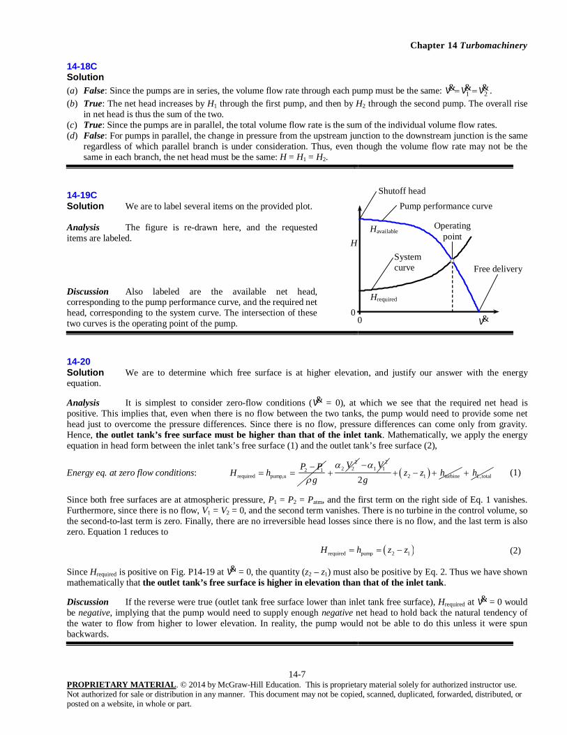
14-19C Solution We are to label several items on the provided plot. Analysis The figure is re-drawn here, and the requested items are labeled. Discussion Also labeled are the available net head, corresponding to the pump performance curve, and the required net head, corresponding to the system curve. The intersection of these two curves is the operating point of the pump.
14-20 Solution We are to determine which free surface is at higher elevation, and justify our answer with the energy equation.
Analysis It is simplest to consider zero-flow conditions (V& = 0), at which we see that the required net head is positive. This implies that, even when there is no flow between the two tanks, the pump would need to provide some net head just to overcome the pressure differences. Since there is no flow, pressure differences can come only from gravity. Hence, the outlet tank’s free surface must be higher than that of the inlet tank. Mathematically, we apply the energy equation in head form between the inlet tank’s free surface (1) and the outlet tank’s free surface (2),
Energy eq. at zero flow conditions: 2 1required pump,u
P PH h
g
22 2V
2
1 1V 2 1 turbine2z z h
g , totalLh (1)
Since both free surfaces are at atmospheric pressure, P1 = P2 = Patm, and the first term on the right side of Eq. 1 vanishes. Furthermore, since there is no flow, V1 = V2 = 0, and the second term vanishes. There is no turbine in the control volume, so the second-to-last term is zero. Finally, there are no irreversible head losses since there is no flow, and the last term is also zero. Equation 1 reduces to
required pump 2 1H h z z (2)
Since Hrequired is positive on Fig. P14-19 at V& = 0, the quantity (z2 – z1) must also be positive by Eq. 2. Thus we have shown mathematically that the outlet tank’s free surface is higher in elevation than that of the inlet tank.
Discussion If the reverse were true (outlet tank free surface lower than inlet tank free surface), Hrequired at V& = 0 would be negative, implying that the pump would need to supply enough negative net head to hold back the natural tendency of the water to flow from higher to lower elevation. In reality, the pump would not be able to do this unless it were spun backwards.
V&
Havailable
Pump performance curve
0 0
Hrequired
System curve
Operating point
H
Free delivery
Shutoff head

Chapter 14 Turbomachinery
14-8 PROPRIETARY MATERIAL. © 2014 by McGraw-Hill Education. This is proprietary material solely for authorized instructor use. Not authorized for sale or distribution in any manner. This document may not be copied, scanned, duplicated, forwarded, distributed, or posted on a website, in whole or part.
14-21 Solution We are to discuss what would happen to the pump performance curve, the system curve, and the operating point if the free surface of the outlet tank were raised to a higher elevation. Analysis The pump is the same pump regardless of the locations of the inlet and outlet tanks’ free surfaces; thus, the pump performance curve does not change. The energy equation is
2 2
2 1 2 2 1 1required pump,u 2 1 turbine2
P P V VH h z z h
g g
, totalLh (1)
Since the only thing that changes is the elevation difference, Eq. 1 shows that Hrequired shifts up as (z2 – z1) increases. Thus, the system curve rises linearly with elevation increase. A plot of H versus V& is plotted, and the new operating point is labeled. Because of the upward shift of the system curve, the operating point moves to a lower value of volume flow rate. Discussion The shift of operating point to lower V& agrees with our physical intuition. Namely, as we raise the elevation of the outlet, the pump has to do more work to overcome gravity, and we expect the flow rate to decrease accordingly.
14-22 Solution We are to discuss what would happen to the pump performance curve, the system curve, and the operating point if a valve changes from 100% to 50% open. Analysis The pump is the same pump regardless of the locations of the inlet and outlet tanks’ free surfaces; thus, the pump performance curve does not change. The energy equation is
2 2
2 1 2 2 1 1required pump,u 2 1 turbine2
P P V VH h z z h
g g
, totalLh (1)
Since both free surfaces are open to the atmosphere, the pressure term vanishes. Since both V1 and V2 are negligibly small at the free surface (the tanks are large), the second term on the right also vanishes. The elevation difference (z2 – z1) does not change, and so the only term in Eq. 1 that is changed by closing the valve is the irreversible head loss term. We know that the minor loss associated with a valve increases significantly as the valve is closed. Thus, the system curve (the curve of Hrequired versus V&) increases more rapidly with volume flow rate (has a larger slope) when the valve is partially closed. A sketch of H versus V& is plotted, and the new operating point is labeled. Because of the higher system curve, the operating point moves to a lower value of volume flow rate, as indicated on the figure. I.e., the volume flow rate decreases.
Discussion The shift of operating point to lower V& agrees with our physical intuition. Namely, as we close the valve somewhat, the pump has to do more work to overcome the losses, and we expect the flow rate to decrease accordingly.
V&
Havailable
Pump performance curve (does not change)
0 0
Hrequired
New system curve
Original operating point
H
Free delivery
Original system curve
New operating point
V&
Havailable
Pump performance curve (does not change)
0 0
Hrequired
New system curve
Original operating point H
Free delivery
Original system curve
New operating point
Chapter 14 Turbomachinery
14-9 PROPRIETARY MATERIAL. © 2014 by McGraw-Hill Education. This is proprietary material solely for authorized instructor use. Not authorized for sale or distribution in any manner. This document may not be copied, scanned, duplicated, forwarded, distributed, or posted on a website, in whole or part.
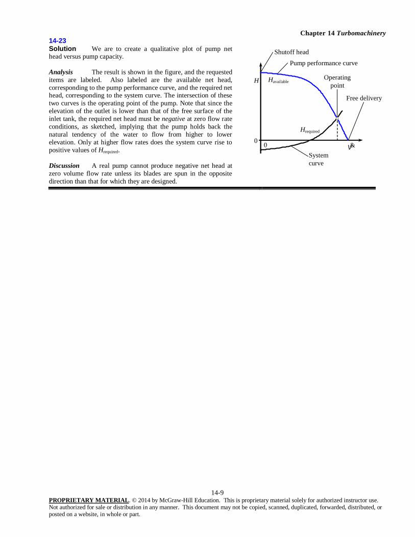
14-23 Solution We are to create a qualitative plot of pump net head versus pump capacity. Analysis The result is shown in the figure, and the requested items are labeled. Also labeled are the available net head, corresponding to the pump performance curve, and the required net head, corresponding to the system curve. The intersection of these two curves is the operating point of the pump. Note that since the elevation of the outlet is lower than that of the free surface of the inlet tank, the required net head must be negative at zero flow rate conditions, as sketched, implying that the pump holds back the natural tendency of the water to flow from higher to lower elevation. Only at higher flow rates does the system curve rise to positive values of Hrequired. Discussion A real pump cannot produce negative net head at zero volume flow rate unless its blades are spun in the opposite direction than that for which they are designed.
V&
Havailable
Pump performance curve
0 0
Hrequired
System curve
Operating point
H
Free delivery
Shutoff head
Chapter 14 Turbomachinery
14-10 PROPRIETARY MATERIAL. © 2014 by McGraw-Hill Education. This is proprietary material solely for authorized instructor use. Not authorized for sale or distribution in any manner. This document may not be copied, scanned, duplicated, forwarded, distributed, or posted on a website, in whole or part.
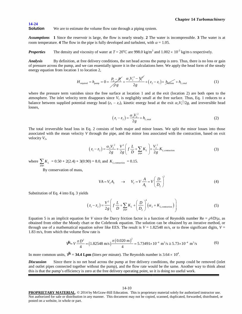
14-24 Solution We are to estimate the volume flow rate through a piping system. Assumptions 1 Since the reservoir is large, the flow is nearly steady. 2 The water is incompressible. 3 The water is at room temperature. 4 The flow in the pipe is fully developed and turbulent, with = 1.05. Properties The density and viscosity of water at T = 20oC are 998.0 kg/m3 and 1.002 10-3 kg/ms respectively. Analysis By definition, at free delivery conditions, the net head across the pump is zero. Thus, there is no loss or gain of pressure across the pump, and we can essentially ignore it in the calculations here. We apply the head form of the steady energy equation from location 1 to location 2,
2 1required pump 0
P PH h
g
2 22 2 1V V
2 1 turbine2z z h
g , totalLh (1)
where the pressure term vanishes since the free surface at location 1 and at the exit (location 2) are both open to the atmosphere. The inlet velocity term disappears since V1 is negligibly small at the free surface. Thus, Eq. 1 reduces to a balance between supplied potential energy head (z1 – z2), kinetic energy head at the exit 2V2
2/2g, and irreversible head losses,
2
2 21 2 ,total2 L
Vz z h
g
(2)
The total irreversible head loss in Eq. 2 consists of both major and minor losses. We split the minor losses into those associated with the mean velocity V through the pipe, and the minor loss associated with the contraction, based on exit velocity V2,
2 22
2 2 21 2 ,contraction
pipe2 2 2L LV VV Lz z f K Kg g D g
(3)
where pipe
LK = 0.50 + 2(2.4) + 3(0.90) = 8.0, and ,contractionLK = 0.15.
By conservation of mass,
2
2 2 22 2
A DVA V A V V VA D
(4)
Substitution of Eq. 4 into Eq. 3 yields
42
1 2 2 ,contractionpipe 22 L L
V L Dz z f K Kg D D
(5)
Equation 5 is an implicit equation for V since the Darcy friction factor is a function of Reynolds number Re = VD/, as obtained from either the Moody chart or the Colebrook equation. The solution can be obtained by an iterative method, or through use of a mathematical equation solver like EES. The result is V = 1.82548 m/s, or to three significant digits, V = 1.83 m/s, from which the volume flow rate is
224 3 4 30.020 m
1.82548 m/s 5.73491 10 m /s 5.73 10 m /s4 4DV
&V (6)
In more common units, V& = 34.4 Lpm (liters per minute). The Reynolds number is 3.64 104.
Discussion Since there is no net head across the pump at free delivery conditions, the pump could be removed (inlet and outlet pipes connected together without the pump), and the flow rate would be the same. Another way to think about this is that the pump’s efficiency is zero at the free delivery operating point, so it is doing no useful work.

Chapter 14 Turbomachinery
14-11 PROPRIETARY MATERIAL. © 2014 by McGraw-Hill Education. This is proprietary material solely for authorized instructor use. Not authorized for sale or distribution in any manner. This document may not be copied, scanned, duplicated, forwarded, distributed, or posted on a website, in whole or part.
14-25 Solution We are to calculate the volume flow rate through a piping system in which the pipe is rough.
Assumptions 1 Since the reservoir is large, the flow is nearly steady. 2 The water is incompressible. 3 The water is at room temperature. 4 The flow in the pipe is fully developed and turbulent, with = 1.05.
Properties The density and viscosity of water at T = 20oC are 998.0 kg/m3 and 1.002 10-3 kg/ms respectively.
Analysis The relative pipe roughness is /D = (0.012 cm)/(2.0 cm) = 0.006 (very rough, as seen on the Moody chart). The calculations are identical to that of the previous problem, except for the pipe roughness. The result is V = 1.6705 m/s, or to three significant digits, V = 1.67 m/s, from which the volume flow rate is 5.25 10-4 m3/s, or V& = 31.5 Lpm. The Reynolds number is 3.33 104. The volume flow rate is lower by about 8.4% compared to the smooth pipe case. This agrees with our intuition, since pipe roughness leads to more pressure drop at a given flow rate.
Discussion If the calculations of the previous problem are done on a computer, it is trivial to change for the present calculations.
14-26 Solution For a given pump and piping system, we are to calculate the volume flow rate and compare with that calculated for Problem 14-24.
Assumptions 1 Since the reservoir is large, the flow is nearly steady. 2 The water is incompressible. 3 The water is at room temperature. 4 The flow in the pipe is fully developed and turbulent, with = 1.05.
Properties The density and viscosity of water at T = 20oC are 998.0 kg/m3 and 1.002 10-3 kg/ms respectively.
Analysis The calculations are identical to those of the previous problem except that the pump’s net head is not zero, but instead is given in the problem statement. At the operating point, we match Havailable to Hrequired, yielding
42
2available required 0 2 ,contraction 1 2
pipe 2
2 L LV L DH H H a f K K z z
g D D
V& (1)
We re-write the second term on the left side of Eq. 1 in terms of average pipe velocity V instead of volume flow rate, since V& = VD2/4, and solve for V,
0 1 24 2 4
2 ,contractionpipe 2
12 16L L
H z zV
L D Df K K ag D D
(2)
Equation 2 is an implicit equation for V since the Darcy friction factor is a function of Reynolds number Re = VD/, as obtained from either the Moody chart or the Colebrook equation. The solution can be obtained by an iterative method, or through use of a mathematical equation solver like EES. The result is V = 2.9293 m/s, from which the volume flow rate is
22 340.020 m m2.9293 m/s 9.203 10
4 4 sDV
&V (3)
In more common units, V& = 55.2 Lpm, an increase of about 60% compared to the flow rate with the pump operating at free delivery. This agrees with our expectations – adding a pump in the line produces a higher flow rate.
Discussion Although there was a pump in the previous problem as well, it was operating at free delivery conditions, implying that it was not contributing anything to the flow – that pump could be removed from the system with no change in flow rate. Here, however, the net head across the pump is about 6.82 m, implying that it is contributing useful head to the flow (in addition to the gravity head already present).

Chapter 14 Turbomachinery
14-12 PROPRIETARY MATERIAL. © 2014 by McGraw-Hill Education. This is proprietary material solely for authorized instructor use. Not authorized for sale or distribution in any manner. This document may not be copied, scanned, duplicated, forwarded, distributed, or posted on a website, in whole or part.
14-27 Solution We are to calculate the volume flow rate through a piping system in which the pipe is rough.
Assumptions 1 Since the reservoir is large, the flow is nearly steady. 2 The water is incompressible. 3 The water is at room temperature. 4 The flow in the pipe is fully developed and turbulent, with = 1.05.
Properties The density and viscosity of water at T = 20oC are 998.0 kg/m3 and 1.002 10-3 kg/ms respectively.
Analysis The relative pipe roughness is /D = (0.012 cm)/(2.0 cm) = 0.006 (very rough, as seen on the Moody chart). The calculations are identical to that of the previous problem, except for the pipe roughness. The result is V = 2.786 m/s, from which the volume flow rate is 8.753 10-4 m3/s, or V& = 52.5 Lpm. The Reynolds number is 5.55 104. The volume flow rate is lower by about 4.9% compared to the smooth pipe case. This agrees with our intuition, since pipe roughness leads to more pressure drop at a given flow rate.
Discussion If the calculations of the previous problem are done on a computer, it is trivial to change for the present calculations.
14-28 Solution We are to calculate pump efficiency and estimate the BEP conditions. Properties The density of water at 20oC is 998.0 kg/m3. Analysis (a) Pump efficiency is
Pump efficiency: pumpg Hbhp
V& (1)
We show the second row of data (at V& = 6.0 Lpm) as an example – the rest are calculated in a spreadsheet for convenience,
3 2 3 2
pump
998.0 kg/m 9.81 m/s 6.0 L/min 46.2 m 1 m 1 min N s W s 0.319 31.9%142 W 1000 L 60 s kg m N m
The results for all rows are shown in Table 1.
(b) The best efficiency point (BEP) occurs at approximately the fourth row of data: * V& 18.0 Lpm, H* = 36.2 m of head, bhp* = 164. W, and pump* = 64.8%. Discussion A more precise BEP could be obtained by curve-fitting the data, as in the next problem.
TABLE 1 Pump performance data for water at 20oC.
V& (Lpm)
H (m)
bhp (W)
pump (%)
0.0 47.5 133 0.0 6.0 46.2 142 31.9
12.0 42.5 153 54.4 18.0 36.2 164 64.8 24.0 26.2 172 59.7 30.0 15.0 174 42.2 36.0 0.0 174 0.0

Chapter 14 Turbomachinery
14-13 PROPRIETARY MATERIAL. © 2014 by McGraw-Hill Education. This is proprietary material solely for authorized instructor use. Not authorized for sale or distribution in any manner. This document may not be copied, scanned, duplicated, forwarded, distributed, or posted on a website, in whole or part.
14-29
Solution We are to generate least-squares polynomial curve fits of a pump’s performance curves, plot the curves, and calculate the BEP. Properties The density of water at 20oC is 998.0 kg/m3. Analysis The efficiencies for each data point in Table P14-31 were calculated in the previous problem. We use Regression analysis to generate the least-squares fits. The equation and coefficients for H are
2 2
0 0
0
47.6643 m 0.0366453 m/Lpm
Or, to 3 significant digits,
H H a H aH a
V&247.7 m 0.0366 m/Lpm
The equation and coefficients for bhp are
2
0 1 2 0
1 2
131. W
bhp bhp a a bhpa a
V V& &22.37 W/Lpm -0.0317 W/Lpm
The equation and coefficients for pump are
2 3
pump pump,0 1 2 3 pump,0
1 2 3
0.152%
a a a
a a a
V V V& & &
2 35.87 %/Lpm -0.0905 %/Lpm -0.00201 %/Lpm
The tabulated data are plotted in Fig. 1 as symbols only. The fitted data are plotted on the same plots as lines only. The agreement is excellent. The best efficiency point is obtained by differentiating the curve-fit expression for pump with respect to volume flow rate, and setting the derivative to zero (solving the resulting quadratic equation for
*V& ),
pump 21 2 32 3 =0 * 19.6 Lpm
da a a
d
V V VV
& & &&
At this volume flow rate, the curve-fitted expressions for H, bhp, and pump yield the operating conditions at the best efficiency point (to three digits each):
* , * , * , *H bhp V& 19.6 Lpm 33.6 m 165 W 65.3%
Discussion This BEP is more precise than that of the previous problem because of the curve fit. The other root of the quadratic is negative obviously not the correct choice.
0
10
20
30
40
50
0 10 20 30 40120
130
140
150
160
170
180
V& (Lpm)
H (m)
bhp (W)
(a)
0
10
20
30
40
50
60
70
0 10 20 30 40
V& (Lpm)
pump (%)
(b)
FIGURE 1 Pump performance curves: (a) H and bhp versus V&, and (b) pump versus V&.

Chapter 14 Turbomachinery
14-14 PROPRIETARY MATERIAL. © 2014 by McGraw-Hill Education. This is proprietary material solely for authorized instructor use. Not authorized for sale or distribution in any manner. This document may not be copied, scanned, duplicated, forwarded, distributed, or posted on a website, in whole or part.
14-30 Solution For a given pump and system requirement, we are to estimate the operating point.
Assumptions 1 The flow is steady. 2 The water is at 20oC and is incompressible.
Analysis The operating point is the volume flow rate at which Hrequired = Havailable. We set the given expression for Hrequired to the curve fit expression of the previous problem, Havailable = H0 a 2V& , and obtain
Operating point: Lpm 21.7
Lpm 6987.21m/Lpm 0.0185)(0.0366453
m 21.7m 47.6643)(2
120
bazzH
V
At this volume flow rate, we use the curve fit to estimate the head, Operating point: m 30.4 m 4105.30)Lpm 6987.21)(m/Lpm 0.0366453(m 47.6643 22
00 V- aHH
Discussion At this operating point, the flow rate is higher than that at the BEP.
14-31E Solution We are to calculate pump efficiency and estimate the BEP conditions. Properties The density of water at 77oF is 62.24 lbm/ft3. Analysis (a) Pump efficiency is
Pump efficiency: pumpg Hbhp
V& (1)
We show the second row of data (at V& = 4.0 gpm) as an example – the rest are calculated in a spreadsheet for convenience,
33 22
pump
ft gal62.24 lbm/ft 32.2 4.0 18.5 ft0.1337 ft 1 min lbf s hp smins 0.292
0.064 hp gal 60 s 32.2 lbm ft 550 ft lbf
or 29.2%. The results for all rows are shown in the table.
(b) The best efficiency point (BEP) occurs at approximately the fourth row of data: * V& 12.0 gpm, H* = 14.5 ft of head, bhp* = 0.074 hp, and pump* = 59.3%. Discussion A more precise BEP could be obtained by curve-fitting the data, as in Problem 14-29.
Pump performance data for water at 77oF.
V& (gpm) H (ft)
bhp (hp)
pump (%)
0.0 19.0 0.06 0.0 4.0 18.5 0.064 29.2 8.0 17.0 0.069 49.7
12.0 14.5 0.074 59.3 16.0 10.5 0.079 53.6 20.0 6.0 0.08 37.8 24.0 0 0.078 0.0
Chapter 14 Turbomachinery
14-15 PROPRIETARY MATERIAL. © 2014 by McGraw-Hill Education. This is proprietary material solely for authorized instructor use. Not authorized for sale or distribution in any manner. This document may not be copied, scanned, duplicated, forwarded, distributed, or posted on a website, in whole or part.
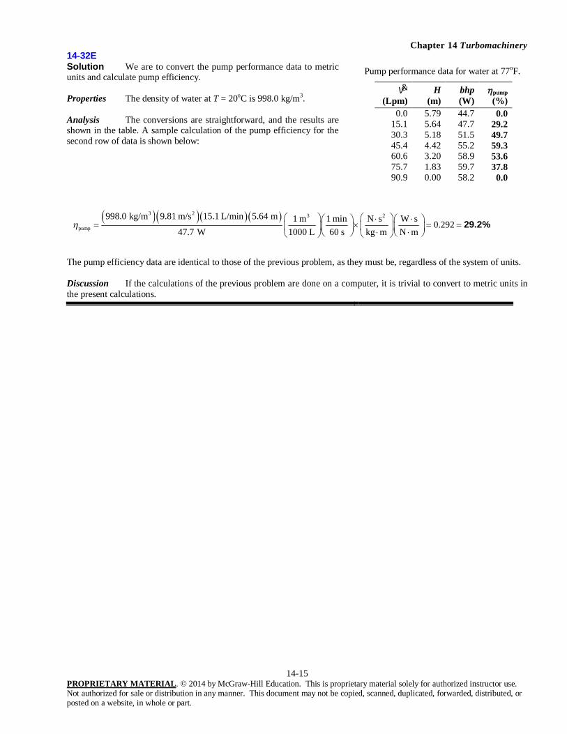
14-32E Solution We are to convert the pump performance data to metric units and calculate pump efficiency. Properties The density of water at T = 20oC is 998.0 kg/m3. Analysis The conversions are straightforward, and the results are shown in the table. A sample calculation of the pump efficiency for the second row of data is shown below:
3 2 3 2
pump
998.0 kg/m 9.81 m/s 15.1 L/min 5.64 m 1 m 1 min N s W s 0.29247.7 W 1000 L 60 s kg m N m
29.2%
The pump efficiency data are identical to those of the previous problem, as they must be, regardless of the system of units. Discussion If the calculations of the previous problem are done on a computer, it is trivial to convert to metric units in the present calculations.
Pump performance data for water at 77oF.
V& (Lpm)
H (m)
bhp (W)
pump (%)
0.0 5.79 44.7 0.0 15.1 5.64 47.7 29.2 30.3 5.18 51.5 49.7 45.4 4.42 55.2 59.3 60.6 3.20 58.9 53.6 75.7 1.83 59.7 37.8 90.9 0.00 58.2 0.0
Chapter 14 Turbomachinery
14-16 PROPRIETARY MATERIAL. © 2014 by McGraw-Hill Education. This is proprietary material solely for authorized instructor use. Not authorized for sale or distribution in any manner. This document may not be copied, scanned, duplicated, forwarded, distributed, or posted on a website, in whole or part.
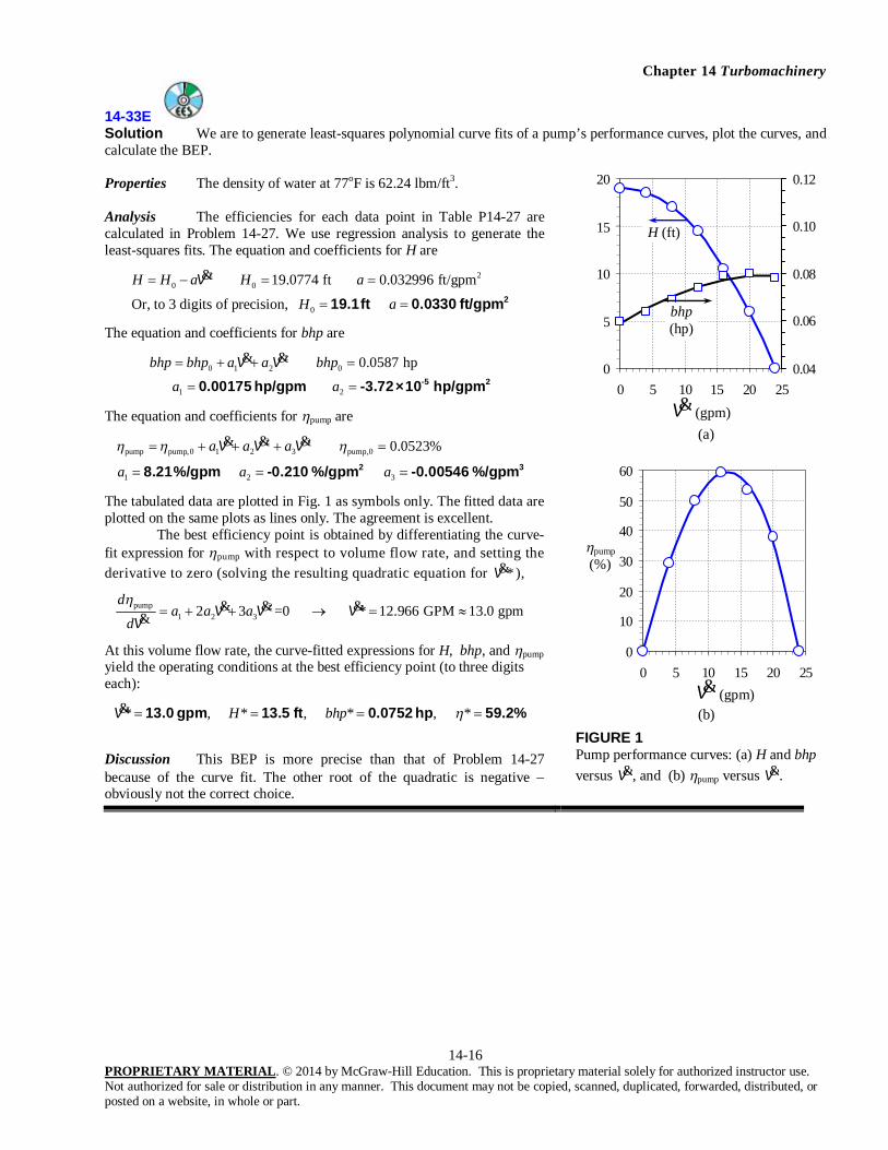
14-33E Solution We are to generate least-squares polynomial curve fits of a pump’s performance curves, plot the curves, and calculate the BEP. Properties The density of water at 77oF is 62.24 lbm/ft3. Analysis The efficiencies for each data point in Table P14-27 are calculated in Problem 14-27. We use regression analysis to generate the least-squares fits. The equation and coefficients for H are
2 2
0 0
0
19.0774 ft 0.032996 ft/gpm
Or, to 3 digits of precision,
H H a H aH a
V&219.1 ft 0.0330 ft/gpm
The equation and coefficients for bhp are
2
0 1 2 0
1 2
0.0587 hp
bhp bhp a a bhpa a
V V& &-5 20.00175 hp/gpm -3.72×10 hp/gpm
The equation and coefficients for pump are
2 3
pump pump,0 1 2 3 pump,0
1 2 3
0.0523%
a a a
a a a
V V V& & &
2 38.21 %/gpm -0.210 %/gpm -0.00546 %/gpm
The tabulated data are plotted in Fig. 1 as symbols only. The fitted data are plotted on the same plots as lines only. The agreement is excellent. The best efficiency point is obtained by differentiating the curve-fit expression for pump with respect to volume flow rate, and setting the derivative to zero (solving the resulting quadratic equation for *V& ),
pump 21 2 32 3 =0 * 12.966 GPM 13.0 gpm
da a a
d
V V VV
& & &&
At this volume flow rate, the curve-fitted expressions for H, bhp, and pump yield the operating conditions at the best efficiency point (to three digits each):
* , * , * , *H bhp V& 13.0 gpm 13.5 ft 0.0752 hp 59.2%
Discussion This BEP is more precise than that of Problem 14-27 because of the curve fit. The other root of the quadratic is negative obviously not the correct choice.
0
5
10
15
20
0 5 10 15 20 250.04
0.06
0.08
0.10
0.12
V& (gpm)
H (ft)
bhp (hp)
(a)
0
10
20
30
40
50
60
0 5 10 15 20 25
V& (gpm)
pump (%)
(b)
FIGURE 1 Pump performance curves: (a) H and bhp versus V&, and (b) pump versus V&.
Chapter 14 Turbomachinery
14-17 PROPRIETARY MATERIAL. © 2014 by McGraw-Hill Education. This is proprietary material solely for authorized instructor use. Not authorized for sale or distribution in any manner. This document may not be copied, scanned, duplicated, forwarded, distributed, or posted on a website, in whole or part.
14-34E Solution For a given pump and system requirement, we are to estimate the operating point. Assumptions 1 The flow is steady. 2 The water is at 77oF and is incompressible. Analysis The operating point is the volume flow rate at which Hrequired = Havailable. We set the given expression for Hrequired to the curve fit expression of Problem 14-26, Havailable = H0 a 2V& , and obtain
Operating point: gpm 13.5
2120
ft/gpm 0.00986)(0.032996ft 11.3-ft 19.0774)(
bazzH
V
At this volume flow rate, the net head of the pump is 13.1 ft. Discussion At this operating point, the flow rate is lower than that at the BEP.
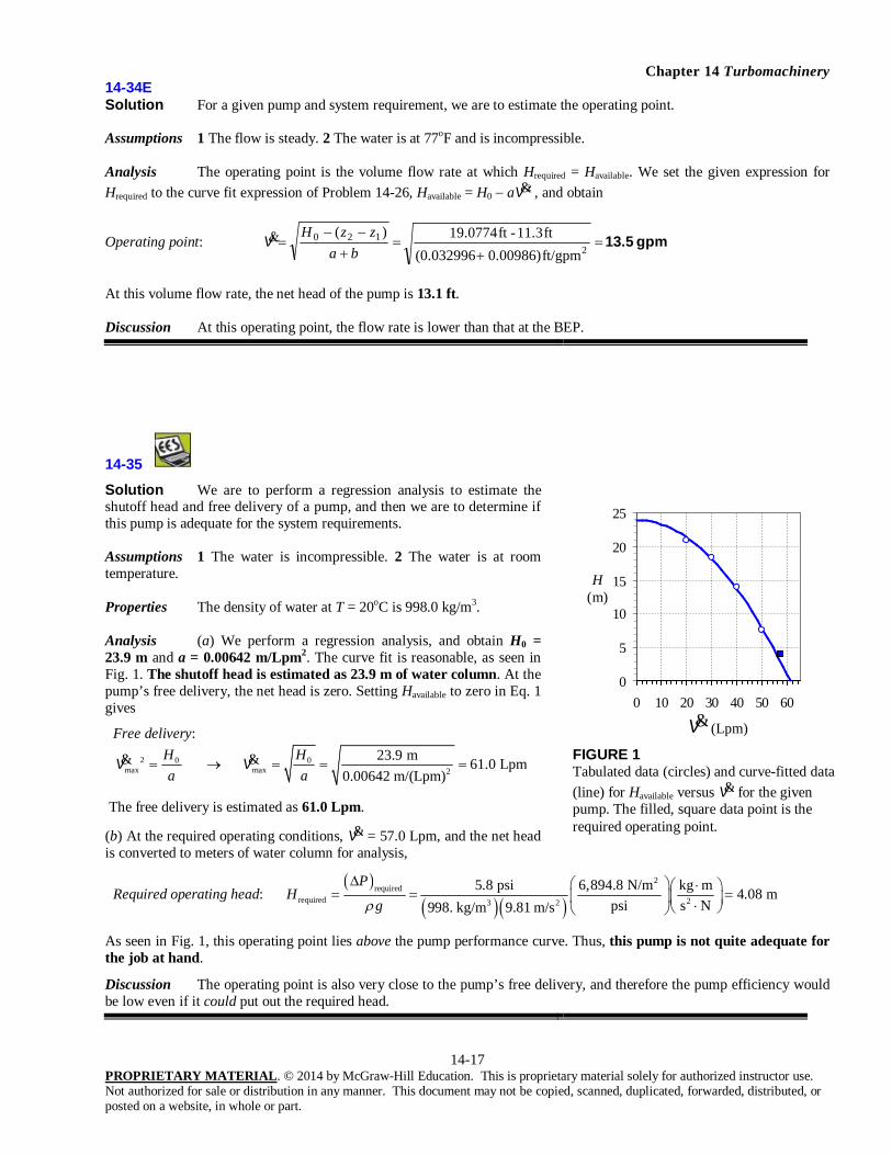
14-35
Solution We are to perform a regression analysis to estimate the shutoff head and free delivery of a pump, and then we are to determine if this pump is adequate for the system requirements. Assumptions 1 The water is incompressible. 2 The water is at room temperature. Properties The density of water at T = 20oC is 998.0 kg/m3. Analysis (a) We perform a regression analysis, and obtain H0 = 23.9 m and a = 0.00642 m/Lpm2. The curve fit is reasonable, as seen in Fig. 1. The shutoff head is estimated as 23.9 m of water column. At the pump’s free delivery, the net head is zero. Setting Havailable to zero in Eq. 1 gives
Free delivery:
2 0 0max max 2
23.9 m 61.0 Lpm0.00642 m/(Lpm)
H Ha a
V V& &
The free delivery is estimated as 61.0 Lpm.
(b) At the required operating conditions, V& = 57.0 Lpm, and the net head is converted to meters of water column for analysis,
Required operating head:
2
requiredrequired 23 2
5.8 psi 6,894.8 N/m kg m 4.08 mpsi s N998. kg/m 9.81 m/s
PH
g
As seen in Fig. 1, this operating point lies above the pump performance curve. Thus, this pump is not quite adequate for the job at hand.
Discussion The operating point is also very close to the pump’s free delivery, and therefore the pump efficiency would be low even if it could put out the required head.
0
5
10
15
20
25
0 10 20 30 40 50 60
V& (Lpm)
H (m)
FIGURE 1 Tabulated data (circles) and curve-fitted data (line) for Havailable versus V& for the given pump. The filled, square data point is the required operating point.

Chapter 14 Turbomachinery
14-18 PROPRIETARY MATERIAL. © 2014 by McGraw-Hill Education. This is proprietary material solely for authorized instructor use. Not authorized for sale or distribution in any manner. This document may not be copied, scanned, duplicated, forwarded, distributed, or posted on a website, in whole or part.
14-36 Solution We are to calculate the operating point of a given pipe/pump system.
Assumptions 1 The water is incompressible. 2 The flow is steady since the reservoirs are large. 3 The water is at room temperature.
Properties The density and viscosity of water at T = 20oC are 998.0 kg/m3 and 1.002 10-3 kg/ms respectively, but these properties are not actually needed in the analysis.
Analysis The operating point is obtained by matching the pump’s performance curve to the system curve,
Operating point: 2 2available 0 required 2 1H H a H z z b V V& &
from which we solve for the volume flow rate (capacity) at the operating point,
0 2 1
operating 2
7.46 m 3.52 m0.0453 0.0261 m/Lpm
H z za b
7.43 Lpm&V
and for the net pump head at the operating point,
0 2 1
operating
7.46 m 0.0261 m 0.0453 m 3.52 m0.0453 m 0.0261 m
H b a z zH
a b
4.96 m
Discussion The water properties and are not needed because the system curve (Hrequired versus V&) is provided here.
14-37 Solution We are to calculate the operating point of a given pipe/pump system. Assumptions 1 The water is incompressible. 2 The flow is steady since the reservoirs are large. 3 The water is at room temperature. Properties The density and viscosity of water at T = 20oC are 998.0 kg/m3 and 1.002 10-3 kg/ms respectively, but these properties are not actually needed in the analysis. Analysis The operating point is obtained by matching the pump’s performance curve to the system curve,
Operating point: 2 2available 0 required 2 1H H a H z z b V V& &
from which we solve for the volume flow rate (capacity) at the operating point,
0 2 1
operating 2
8.13 m 3.52 m0.0297 0.0261 m/Lpm
H z za b
9.09 Lpm&V
and for the net pump head at the operating point,
0 2 1
operating
8.13 m 0.0261 m 0.0297 m 3.52 m0.0297 m 0.0261 m
H b a z zH
a b
5.68 m
This represents an improvement in flow rate of about 22%, and YES, it meets the requirement.
Discussion The water properties and are not needed because the system curve (Hrequired versus V&) is provided here.

Chapter 14 Turbomachinery
14-19 PROPRIETARY MATERIAL. © 2014 by McGraw-Hill Education. This is proprietary material solely for authorized instructor use. Not authorized for sale or distribution in any manner. This document may not be copied, scanned, duplicated, forwarded, distributed, or posted on a website, in whole or part.
14-38E Solution We are to find the units of coefficient a, write maxV& in terms of H0 and a, and calculate the operating point of the pump. Assumptions 1 The flow is steady. 2 The water is incompressible. Analysis (a) Solving the given expression for a gives
Coefficient a: 0 available2
H Ha
V& 2
ftunits of gpm
a (1)
(b) At the pump’s free delivery, the net head is zero. Setting Havailable to zero in the given expression gives
Free delivery: 2 0max
Ha
V& 0max
Ha
V& (2)
(c) The operating point is obtained by matching the pump’s performance curve to the system curve. Equating these gives
2 2available 0 required 2 1H H a H z z b V V& & (3)
After some algebra, Eq. 3 reduces to
Operating point capacity: 0 2 1
operating
H z za b
V& (4)
and the net pump head at the operating point is obtained by plugging Eq. 4 into the given expression,
Operating point pump head: 0 2 1
operating
H b a z zH
a b
(5)
Discussion Equation 4 reveals that H0 must be greater than elevation difference (z2 – z1) in order to have a valid operating point. This agrees with our intuition, since the pump must be able to overcome the gravitational head between the tanks.
Chapter 14 Turbomachinery
14-20 PROPRIETARY MATERIAL. © 2014 by McGraw-Hill Education. This is proprietary material solely for authorized instructor use. Not authorized for sale or distribution in any manner. This document may not be copied, scanned, duplicated, forwarded, distributed, or posted on a website, in whole or part.
14-39E Solution For a given pump and system, we are to calculate the capacity. Assumptions 1 The water is incompressible. 2 The flow is nearly steady since the reservoirs are large. 3 The water is at room temperature. Properties The kinematic viscosity of water at T = 68oF is 1.055 10-5 ft2/s. Analysis We apply the energy equation in head form between the inlet reservoir’s free surface (1) and the outlet reservoir’s free surface (2),
2 1required pump,u
P PH h
g
22 2V
2
1 1V 2 1 turbine2z z h
g , totalLh (1)
Since both free surfaces are at atmospheric pressure, P1 = P2 = Patm, and the first term on the right side of Eq. 1 vanishes. Furthermore, since there is no flow, V1 = V2 = 0, and the second term also vanishes. There is no turbine in the control volume, so the second-to-last term is zero. Finally, the irreversible head losses are composed of both major and minor losses, but the pipe diameter is constant throughout. Equation 1 therefore reduces to
2
required 2 1 ,total 2 1 2L LL VH z z h z z f KD g
(2)
The dimensionless roughness factor is /D = 0.0011/1.20 = 9.17 10-4, and the sum of all the minor loss coefficients is
0.5 2.0 6.8 3 0.34 1.05 11.37LK
The pump/piping system operates at conditions where the available pump head equals the required system head. Thus, we equate the given expression and Eq. 2 to find the operating point,
2 4 2
2available required 0 2 1
16 2LD L VH H H a V z z f K
D g
(3)
where we have written the volume flow rate in terms of average velocity through the pipe,
Volume flow rate in terms of average velocity: 2
4DV
V& (4)
Equation 3 is an implicit equation for V since the Darcy friction factor f is a function of Reynolds number Re = VD/ = VD/, as obtained from either the Moody chart or the Colebrook equation. The solution can be obtained by an iterative method, or through use of a mathematical equation solver like EES. The result is V = 1.80 ft/s, from which the volume flow rate is V& = 6.34 gpm. The Reynolds number is 1.67 104. Discussion We verify our results by comparing Havailable (given) and Hrequired (Eq. 2) at this flow rate: Havailable = 24.4 ft and Hrequired = 24.4 ft.

Chapter 14 Turbomachinery
14-21 PROPRIETARY MATERIAL. © 2014 by McGraw-Hill Education. This is proprietary material solely for authorized instructor use. Not authorized for sale or distribution in any manner. This document may not be copied, scanned, duplicated, forwarded, distributed, or posted on a website, in whole or part.
14-40E Solution We are to plot Hrequired and Havailable versus V&, and indicate the operating point. Analysis We use the equations of the previous problem, with the same constants and parameters, to generate the plot shown. The operating point is the location where the two curves intersect. The values of H and V&at the operating point match those of the previous problem, as they should. Discussion A plot like this, in fact, is an alternate method of obtaining the operating point. In this case, the curve of Hrequired is fairly flat, indicating that the majority of the required pump head is attributed to elevation change, while a small fraction is attributed to major and minor head losses through the piping system.
14-41E Solution We are to re-calculate volume flow rate for a piping system with a much longer pipe, and we are to compare with the previous results. Analysis All assumptions, properties, dimensions, and parameters are identical to those of the previous problem, except that total pipe length L is longer. We repeat the calculations and find that V = 1.63 ft/s, from which the volume flow rate is V& = 5.75 gpm, and the net head of the pump is 42.3 ft. The Reynolds number for the flow in the pipe is 1.55 104. The volume flow rate has decreased by about 9.3%. Discussion The decrease in volume flow rate is smaller than we may have suspected. This is because the majority of the pump work goes into raising the elevation of the water. In addition, as seen in the plot from the previous problem, the pump performance curve is quite steep near these flow rates – a significant change in required net head leads to a much less significant change in volume flow rate.
0
20
40
60
80
100
120
140
0 2 4 6 8
V& (gpm)
H (ft)
Operating point
Havailable
Hrequired

Chapter 14 Turbomachinery
14-22 PROPRIETARY MATERIAL. © 2014 by McGraw-Hill Education. This is proprietary material solely for authorized instructor use. Not authorized for sale or distribution in any manner. This document may not be copied, scanned, duplicated, forwarded, distributed, or posted on a website, in whole or part.
14-42E
Solution We are to perform a regression analysis to translate tabulated pump performance data into an analytical expression, and then use this expression to predict the volume flow rate through a piping system. Assumptions 1 The water is incompressible. 2 The flow is nearly steady since the reservoirs are large. 3 The water is at room temperature. Properties For water at T = 68oF, = 6.572 10-4 lbm/fts, and = 62.31 lbm/ft3, from which = 1.055 10-5 ft2/s.
Analysis (a) We perform a regression analysis, and obtain H0 = 38.15 ft and a = 0.06599 ft/gpm2. The curve fit is very good, as seen in Fig. 1.
(b) We repeat the calculations of Problem 14-37 with the new pump performance coefficients, and find that V = 3.29 ft/s, from which the volume flow rate is V& = 11.6 gpm, and the net head of the pump is 29.3 ft. The Reynolds number for the flow in the pipe is 3.05 104. The volume flow rate has increased by about 83%. Paul is correct – this pump performs much better, nearly doubling the flow rate.
(c) A plot of net head versus volume flow rate is shown in Fig. 2. Discussion This pump is more appropriate for the piping system at hand.
0 5
10 15 20 25 30 35 40 45
0 5 10 15 20 25
H ( ft )
Curve fit
Data points
V& (gpm)
FIGURE 1 Tabulated data (symbols) and curve-fitted data (line) for Havailable versus V& for the proposed pump.
0
10
20
30
40
0 5 10 15 20 25
V& (gpm)
H (ft)
Operating point
Havailable Hrequired
FIGURE 2 Havailable and Hrequired versus V& for a piping system with pump; the operating point is also indicated, where the two curves meet.

Chapter 14 Turbomachinery
14-23 PROPRIETARY MATERIAL. © 2014 by McGraw-Hill Education. This is proprietary material solely for authorized instructor use. Not authorized for sale or distribution in any manner. This document may not be copied, scanned, duplicated, forwarded, distributed, or posted on a website, in whole or part.
14-43 Solution For a given pump and system, we are to calculate the capacity. Assumptions 1 The water is incompressible. 2 The flow is nearly steady since the reservoirs are large. 3 The water is at room temperature. Properties The density and viscosity of water at T = 20oC are 998.0 kg/m3 and 1.002 10-3 kg/ms respectively. Analysis We apply the energy equation in head form between the inlet reservoir’s free surface (1) and the outlet reservoir’s free surface (2),
2 1required pump,u
P PH h
g
22 2V
2
1 1V 2 1 turbine2z z h
g , totalLh (1)
Since both free surfaces are at atmospheric pressure, P1 = P2 = Patm, and the first term on the right side of Eq. 1 vanishes. Furthermore, since there is no flow, V1 = V2 = 0, and the second term also vanishes. There is no turbine in the control volume, so the second-to-last term is zero. Finally, the irreversible head losses are composed of both major and minor losses, but the pipe diameter is constant throughout. Equation 1 therefore reduces to
2
required 2 1 ,total 2 1 2L LL VH z z h z z f KD g
(2)
The dimensionless roughness factor is
0 25 mm 1 cm 0 01232 03 cm 10 mm. .
D .
The sum of all the minor loss coefficients is
0.5 17.5 5 0.92 1.05 23.65LK
The pump/piping system operates at conditions where the available pump head equals the required system head. Thus, we equate the given expression and Eq. 2 to find the operating point,
2 4 2
2available required 0 2 1
16 2LD L VH H H a V z z f K
D g
(3)
where we have written the volume flow rate in terms of average velocity through the pipe,
2
4DV
V&
Equation 3 is an implicit equation for V since the Darcy friction factor f is a function of Reynolds number Re = VD/, as obtained from either the Moody chart or the Colebrook equation. The solution can be obtained by an iterative method, or through use of a mathematical equation solver like EES. The result is V = 0.59603 0.596 m/s, from which the volume flow rate is V& = 11.6 Lpm. The Reynolds number is 1.21 104. Discussion We verify our results by comparing Havailable (given) and Hrequired (Eq. 2) at this flow rate: Havailable = 15.3 m and Hrequired = 15.3 m.

Chapter 14 Turbomachinery
14-24 PROPRIETARY MATERIAL. © 2014 by McGraw-Hill Education. This is proprietary material solely for authorized instructor use. Not authorized for sale or distribution in any manner. This document may not be copied, scanned, duplicated, forwarded, distributed, or posted on a website, in whole or part.
14-44 Solution We are to plot Hrequired and Havailable versus V&, and indicate the operating point. Analysis We use the equations of the previous problem, with the same constants and parameters, to generate the plot shown. The operating point is the location where the two curves intersect. The values of H and V&at the operating point match those of the previous problem, as they should. Discussion A plot like this, in fact, is an alternate method of obtaining the operating point.
14-45 Solution We are to re-calculate volume flow rate for a piping system with a smaller elevation difference, and we are to compare with the previous results.
Analysis All assumptions, properties, dimensions, and parameters are identical to those of the previous problem, except that the elevation difference between reservoir surfaces (z2 – z1) is smaller. We repeat the calculations and find that V = 0.538 m/s, from which the volume flow rate is V& = 10.5 Lpm, and the net head of the pump is 17.0 m. The Reynolds number for the flow in the pipe is 1.09 104. The volume flow rate has increased by about 9.5%.
Discussion The increase in volume flow rate is modest. This is because only about half of the pump work goes into raising the elevation of the water – the other half goes into overcoming irreversible losses.
0
5
10
15
20
25
30
0 5 10 15 20
V& (Lpm)
H (m)
Operating point
Havailable
Hrequired

Chapter 14 Turbomachinery
14-25 PROPRIETARY MATERIAL. © 2014 by McGraw-Hill Education. This is proprietary material solely for authorized instructor use. Not authorized for sale or distribution in any manner. This document may not be copied, scanned, duplicated, forwarded, distributed, or posted on a website, in whole or part.
14-46
Solution We are to perform a regression analysis to translate tabulated pump performance data into an analytical expression, and then use this expression to predict the volume flow rate through a piping system. Assumptions 1 The water is incompressible. 2 The flow is nearly steady since the reservoirs are large. 3 The water is at room temperature. Properties The density and viscosity of water at T = 20oC are 998.0 kg/m3 and 1.002 10-3 kg/ms respectively.
Analysis (a) We perform a regression analysis, and obtain H0 = 47.6 m and a = 0.05119 m/Lpm2. The curve fit is reasonable, as seen in Fig. 1.
(b) We repeat the calculations of Problem 14-41 with the new pump performance coefficients, and find that V = 1.00 m/s, from which the volume flow rate is V& = 19.5 Lpm, and the net head of the pump is 28.3 m. The Reynolds number for the flow in the pipe is 2.03 104. The volume flow rate has increased by about 69%. April’s goal has not been reached. She will need to search for an even stronger pump.
(c) A plot of net head versus volume flow rate is shown in Fig. 2. Discussion As is apparent from Fig. 2, the required net head increases rapidly with increasing volume flow rate. Thus, doubling the flow rate would require a significantly heftier pump.
0
10
20
30
40
50
0 10 20 30
V& (Lpm)
H (m) Curve fit
Data points
FIGURE 1 Tabulated data (symbols) and curve-fitted data (line) for Havailable versus V& for the proposed pump.
0
10
20
30
40
50
0 5 10 15 20 25 30
V& (Lpm)
H (m) Operating
point
Havailable
Hrequired
FIGURE 2 Havailable and Hrequired versus V& for a piping system with pump; the operating point is also indicated, where the two curves meet.

Chapter 14 Turbomachinery
14-26 PROPRIETARY MATERIAL. © 2014 by McGraw-Hill Education. This is proprietary material solely for authorized instructor use. Not authorized for sale or distribution in any manner. This document may not be copied, scanned, duplicated, forwarded, distributed, or posted on a website, in whole or part.
14-47 Solution We are to calculate the volume flow rate when the pipe diameter of a piping/pump system is doubled. Analysis The analysis is identical to that of Problem 14-41 except for the diameter change. The calculations yield V = 0.19869 0.199 m/s, from which the volume flow rate is V& = 15.4 Lpm, and the net head of the pump is 8.25 m. The Reynolds number for the flow in the pipe is 8.03 103. The volume flow rate has increased by about 33%. This agrees with our intuition since irreversible head losses go down significantly by increasing pipe diameter. Discussion The gain in volume flow rate is significant because the irreversible head losses contribute to about half of the total pump head requirement in the original problem.
14-48 Solution We are to compare Reynolds numbers for a pipe flow system – the second case having a pipe diameter twice that of the first case. Properties The density and viscosity of water at T = 20oC are 998.0 kg/m3 and 1.002 10-3 kg/ms respectively. Analysis From the results of the two problems, the Reynolds number of the first case is
Case 1 (D = 2.03 cm): 3
4-3 3
998 kg/m 0.59603 m/s 0.0203 mRe 1.21 10
1.002 10 kg/mVD
and that of the second case is
Case 2 (D = 4.06 cm): 3
4-3 3
998 kg/m 0.19869 m/s 0.0406 mRe 0.803 10
1.002 10 kg/mVD
Thus, the Reynolds number of the larger diameter pipe is smaller than that of the smaller diameter pipe. This may be somewhat surprising, but since average pipe velocity scales as the inverse of pipe diameter squared, Reynolds number increases linearly with pipe diameter due to the D in the numerator, but decreases quadratically with pipe diameter due to the V in the numerator. The net effect is a decrease in Re with pipe diameter when V& is the same. In this problem, V& increases somewhat as the diameter is doubled, but not enough to increase the Reynolds number. Discussion At first glance, most people would think that Reynolds number increases as both diameter and volume flow rate increase, but this is not always the case.
14-49 Solution We are to compare the volume flow rate in a piping system with and without accounting for minor losses. Analysis The analysis is identical to that of Problem 14-41, except we ignore all the minor losses. The calculations yield V = 0.604 m/s, from which the volume flow rate is V& = 11.7 Lpm, and the net head of the pump is 15.1 m. The Reynolds number for the flow in the pipe is 1.22 104. The volume flow rate has increased by about 1.3%. Thus, minor losses are nearly negligible in this calculation. This agrees with our intuition since the pipe is very long. Discussion Since the Colebrook equation is accurate to at most 5%, a 1.3% change is well within the error. Nevertheless, it is not excessively difficult to include the minor losses, especially when solving the problem on a computer.
Chapter 14 Turbomachinery
14-27 PROPRIETARY MATERIAL. © 2014 by McGraw-Hill Education. This is proprietary material solely for authorized instructor use. Not authorized for sale or distribution in any manner. This document may not be copied, scanned, duplicated, forwarded, distributed, or posted on a website, in whole or part.
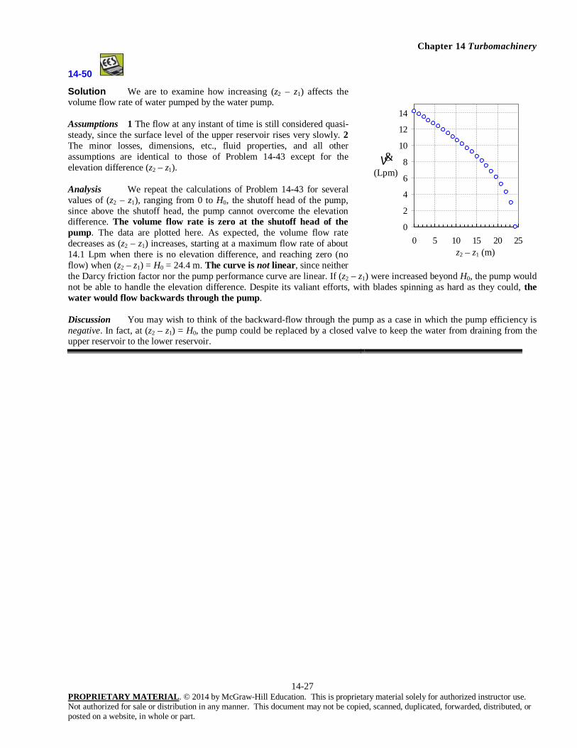
14-50
Solution We are to examine how increasing (z2 – z1) affects the volume flow rate of water pumped by the water pump. Assumptions 1 The flow at any instant of time is still considered quasi-steady, since the surface level of the upper reservoir rises very slowly. 2 The minor losses, dimensions, etc., fluid properties, and all other assumptions are identical to those of Problem 14-43 except for the elevation difference (z2 – z1). Analysis We repeat the calculations of Problem 14-43 for several values of (z2 – z1), ranging from 0 to H0, the shutoff head of the pump, since above the shutoff head, the pump cannot overcome the elevation difference. The volume flow rate is zero at the shutoff head of the pump. The data are plotted here. As expected, the volume flow rate decreases as (z2 – z1) increases, starting at a maximum flow rate of about 14.1 Lpm when there is no elevation difference, and reaching zero (no flow) when (z2 – z1) = H0 = 24.4 m. The curve is not linear, since neither the Darcy friction factor nor the pump performance curve are linear. If (z2 – z1) were increased beyond H0, the pump would not be able to handle the elevation difference. Despite its valiant efforts, with blades spinning as hard as they could, the water would flow backwards through the pump. Discussion You may wish to think of the backward-flow through the pump as a case in which the pump efficiency is negative. In fact, at (z2 – z1) = H0, the pump could be replaced by a closed valve to keep the water from draining from the upper reservoir to the lower reservoir.
0
2
4
6
8
10
12
14
0 5 10 15 20 25
z2 – z1 (m)
V& (Lpm)

Chapter 14 Turbomachinery
14-28 PROPRIETARY MATERIAL. © 2014 by McGraw-Hill Education. This is proprietary material solely for authorized instructor use. Not authorized for sale or distribution in any manner. This document may not be copied, scanned, duplicated, forwarded, distributed, or posted on a website, in whole or part.
14-51 Solution We are to estimate the operating point of a given fan and duct system.
Assumptions 1 The flow is steady and incompressible. 2 The concentration of contaminants is low; the fluid properties are those of air alone. 3 The air is at 25oC and 101,300 Pa. 4 The air flowing in the duct is turbulent with = 1.05.
Properties For air at 25oC, = 1.849 10-5 kg/ms, = 1.184 kg/m3, and = 1.562 10-5 m2/s. The density of water at STP (for conversion to water head) is 997.0 kg/m3.
Analysis We apply the steady energy equation along a streamline from point 1 in the stagnant air region in the room to point 2 at the duct outlet,
2 1required
P PH
g
2 22 2 1 1V V
2 12z z
g , totalLh (1)
P1 is equal to Patm, and P2 is also equal to Patm since the jet discharges into outside air on the roof of the building. Thus the pressure terms cancel out in Eq. 1. We ignore the air speed at point 1 since it is chosen (wisely) far enough away from the hood inlet so that the air is nearly stagnant. Finally, the elevation difference is neglected for gases. Equation 1 reduces to
Required net head: 2
2 2required ,total2 L
VH h
g
(2)
The total head loss in Eq. 2 is a combination of major and minor losses. Since the duct diameter is constant,
Total irreversible head loss: 2
,total 2L LL Vh f KD g
(3)
The required net head of the fan is thus
2
required 2 2LL VH f KD g
(4)
To find the operating point, we equate Havailable and Hrequired, being careful to keep consistent units. Note that the required head in Eq. 4 is expressed naturally in units of equivalent column height of the pumped fluid, which is air in this case. However, the available net head (given) is in terms of equivalent water column height. We convert constants H0 and a in Eq. 1 to mm of air column for consistency by multiplying by the ratio of water density to air density,
water0, mm water water 0, mm air air 0, mm air 0, mm water
air
H H H H
and 2 2water
mm air / LPM mm water / LPMair
a a
We re-write the given expression in terms of average duct velocity rather than volume flow rate,
Available net head: 2 4
2available 0 16
DH H a V (5)
Equating Eqs. 4 and 5 yields the operating point,
2 4 2
2available required 0 2
16 2LD L VH H H a V f K
D g
(6)
The dimensionless roughness factor is /D = 0.15/150 = 1.00 10-3, and the sum of all the minor loss coefficients is 3.3 3 0.21 1.8 0.36 6.6 12.69LK . Note that there is no minor loss associated with the exhaust, since point 2
is at the exit plane of the duct, and does not include irreversible losses associated with the turbulent jet. Equation 6 is an implicit equation for V since the Darcy friction factor is a function of Reynolds number Re = VD/ = VD/, as obtained from the Moody chart or the Colebrook equation. The solution can be obtained by an iterative method, or through use of a mathematical equation solver like EES. The result is V = 6.71 m/s, from which the volume flow rate is V& = 7090 Lpm.
Discussion We verify our results by comparing Havailable (given) and Hrequired (Eq. 5) at this flow rate: Havailable = 47.4 mm of water and Hrequired = 47.4 mm of water, both of which are equivalent to 40.0 m of air column.

Chapter 14 Turbomachinery
14-29 PROPRIETARY MATERIAL. © 2014 by McGraw-Hill Education. This is proprietary material solely for authorized instructor use. Not authorized for sale or distribution in any manner. This document may not be copied, scanned, duplicated, forwarded, distributed, or posted on a website, in whole or part.
14-52 Solution We are to plot Hrequired and Havailable versus V&, and indicate the operating point. Analysis We use the equations of the previous problem, with the same constants and parameters, to generate the plot shown. The operating point is the location where the two curves intersect. The values of H and V&at the operating point match those of the previous problem, as they should. Discussion A plot like this, in fact, is an alternate method of obtaining the operating point. The operating point is at a volume flow rate near the center of the plot, indicating that the fan efficiency is probably reasonably high.
14-53 Solution We are to estimate the volume flow rate at the operating point without accounting for minor losses, and then we are to compare with the previous results. Analysis All assumptions and properties are the same as those of Problem 14-52, except that we ignore all minor losses (we set KL = 0). The resulting volume flow rate at the operating point is V& = 10,900 Lpm (to three significant digits), approximately 54% higher than for the case with minor losses taken into account. In this problem, minor losses are not “minor”, and are by no means negligible. Even though the duct is fairly long (L/D is about 163), the minor losses are large, especially those through the damper and the one-way valve. Discussion An error of 54% is not acceptable in this type of problem. Furthermore, since it is not difficult to account for minor losses, especially if the calculations are performed on a computer, it is wise not to ignore these terms.
14-54 Solution We are to calculate pressure at two locations in a blocked duct system. Assumptions 1 The flow is steady. 2 The concentration of contaminants in the air is low; the fluid properties are those of air alone. 3 The air is at standard temperature and pressure (STP: 25oC and 101,300 Pa), and is incompressible. Properties The density of water at 25oC is 997.0 kg/m3. Analysis Since the air is completely blocked by the one-way valve, there is no flow. Thus, there are no major or minor losses – just a pressure gain across the fan. Furthermore, the fan is operating at its shutoff head conditions. Since the pressure in the room is atmospheric, the gage pressure anywhere in the stagnant air region in the duct between the fan and the one-way valve is therefore equal to H0 = 60.0 mm of water column. We convert to pascals as follows:
Gage pressure at both locations: 2 2
gage water 0 3 2
kg m N s Pa m998 0 9 81 0 060 m 587 Pakg m Nm s
P gH . . .
Thus, at either location, the gage pressure is 60.0 mm of water column, or 587 Pa. Discussion The answer depends only on the shutoff head of the fan – duct diameter, minor losses, etc, are irrelevant for this case since there is no flow. The fan should not be run for long time periods under these conditions, or it may burn out.
0
20
40
60
80
100
0 5000 10000 15000
V& (Lpm)
H (mm)
Operating point
Havailable
Hrequired

Chapter 14 Turbomachinery
14-30 PROPRIETARY MATERIAL. © 2014 by McGraw-Hill Education. This is proprietary material solely for authorized instructor use. Not authorized for sale or distribution in any manner. This document may not be copied, scanned, duplicated, forwarded, distributed, or posted on a website, in whole or part.
14-55E Solution We are to estimate the operating point of a given fan and duct system. Assumptions 1 The flow is steady. 2 The concentration of contaminants in the air is low; the fluid properties are those of air alone. 3 The air is at standard temperature and pressure (STP), and is incompressible. 4 The air flowing in the duct is turbulent with = 1.05. Properties For air at STP (T = 77oF, P = 14.696 psi = 2116.2 lbf/ft2), = 1.242 10-5 lbm/fts, = 0.07392 lbm/ft3, and = 1.681 10-4 ft2/s. The density of water at STP (for conversion to inches of water head) is 62.24 lbm/ft3. Analysis We apply the steady energy equation along a streamline from point 1 in the stagnant air region in the room to point 2 at the duct outlet,
Required net head: 2 1required
P PH
g
2 22 2 1 1V V
2 12z z
g , totalLh (1)
At point 1, P1 is equal to Patm, and at point 2, P2 is also equal to Patm since the jet discharges into the outside air on the roof of the building. Thus the pressure terms cancel out in Eq. 1. We ignore the air speed at point 1 since it is chosen (wisely) far enough away from the hood inlet so that the air is nearly stagnant. Finally, the elevation difference is neglected for gases. Equation 1 reduces to
2
2 2required ,total2 L
VH h
g
(2)
The total head loss in Eq. 2 is a combination of major and minor losses, and depends on volume flow rate. Since the duct diameter is constant,
Total irreversible head loss: 2
,total 2L LL Vh f KD g
(3)
The required net head of the fan is thus
2
required 2 2LL VH f KD g
(4)
To find the operating point, we equate Havailable and Hrequired, being careful to keep consistent units. Note that the required head in Eq. 4 is expressed naturally in units of equivalent column height of the pumped fluid, which is air in this case. However, the available net head (given) is in terms of equivalent water column height. We convert constants H0 and a to inches of air column for consistency by multiplying by the ratio of water density to air density,
water0, inch water water 0, inch air air 0, inch air 0, inch water
air
H H H H
and similarly,
2 2water
inch air / SCFM inch water / SCFMair
a a
We re-write the given expression in terms of average duct velocity rather than volume flow rate,
Available net head: 2 4
2available 0 16
DH H a V (5)
again taking care to keep consistent units. Equating Eqs. 4 and 5 yields
Operating point: 2 4 2
2available required 0 2
16 2LD L VH H H a V f K
D g
(6)

Chapter 14 Turbomachinery
14-31 PROPRIETARY MATERIAL. © 2014 by McGraw-Hill Education. This is proprietary material solely for authorized instructor use. Not authorized for sale or distribution in any manner. This document may not be copied, scanned, duplicated, forwarded, distributed, or posted on a website, in whole or part.
The dimensionless roughness factor is /D = 0.0059/9.06 = 6.52 10-4, and the sum of all the minor loss coefficients is
Minor losses: 4.6 3 0.21 1.8 7.03LK
Note that there is no minor loss associated with the exhaust, since point 2 is taken at the exit plane of the duct, and does not include irreversible losses associated with the turbulent jet. Equation 6 is an implicit equation for V since the Darcy friction factor is a function of Reynolds number Re = VD/ = VD/, as obtained from either the Moody chart or the Colebrook equation. The solution can be obtained by an iterative method, or through use of a mathematical equation solver like EES. The result is V = 16.8 ft/s, from which the volume flow rate is V& = 452 SCFM. The Reynolds number is 7.63 104. Discussion We verify our results by comparing Havailable (Eq. 1) and Hrequired (Eq. 5) at this flow rate: Havailable = 0.566 inches of water and Hrequired = 0.566 inches of water.

Chapter 14 Turbomachinery
14-32 PROPRIETARY MATERIAL. © 2014 by McGraw-Hill Education. This is proprietary material solely for authorized instructor use. Not authorized for sale or distribution in any manner. This document may not be copied, scanned, duplicated, forwarded, distributed, or posted on a website, in whole or part.
14-56E Solution We are to calculate the value of KL, damper such that the volume flow rate through the duct decreases by a factor of 3. Analysis All assumptions and properties are the same as those of the previous problem. We set the volume flow rate to V& = 452/3 = 150.7 SCFM, one-half of the previous result, and solve for KL, damper. The result is KL, damper = 295, significantly higher than the value of 1.8 for the fully open case. Discussion Because of the nonlinearity of the problem, we cannot simply double the damper’s loss coefficient in order to decrease the flow rate by a factor of three. Indeed, the minor loss coefficient must be increased by a factor of more than 160. If a computer was used for the calculations of the previous problem, the solution here is most easily obtained by trial and error.
14-57E Solution We are to estimate the volume flow rate at the operating point without accounting for minor losses, and then we are to compare with the previous results. Analysis All assumptions and properties are the same as those of Problem 14-49, except that we ignore all minor losses (we set KL = 0). The resulting volume flow rate at the operating point is V& = 503 SCFM, approximately 11% higher than for the case with minor losses taken into account. In this problem, minor losses are indeed “minor”, although they are not negligible. We should not be surprised at this result, since there are several minor losses, and the duct is not extremely long (L/D is only 45.0). Discussion An error of 11% may be acceptable in this type of problem. However, since it is not difficult to account for minor losses, especially if the calculations are performed on a computer, it is wise not to ignore these terms.

Chapter 14 Turbomachinery
14-33 PROPRIETARY MATERIAL. © 2014 by McGraw-Hill Education. This is proprietary material solely for authorized instructor use. Not authorized for sale or distribution in any manner. This document may not be copied, scanned, duplicated, forwarded, distributed, or posted on a website, in whole or part.
14-58E Solution For a given pump and piping system we are to estimate the maximum volume flow rate that can be pumped without cavitation. Assumptions 1 The flow is steady. 2 The water is incompressible. 3 The flow is turbulent. Properties Patm = 14.696 psi = 2116.2 lbf/ft2. For water at T = 77oF, = 6.002 10-4 lbm/(fts), = 62.24 lbm/ft3, and Pv = 66.19 lbf/ft2. Analysis We apply the steady energy equation in head form along a streamline from point 1 at the reservoir surface to point 2 at the pump inlet,
2
1 1 1
2P Vg g
1 pump,uz h 2
2 2 22 turbine2
P Vz h
g g
, totalLh (1)
In Eq. 1 we have ignored the water speed at the reservoir surface (V1 0). There is no turbine in the piping system. Also, although there is a pump in the system, there is no pump between point 1 and point 2; hence the pump head term also drops out. We solve Eq. 1 for P2/(g), which is the pump inlet pressure expressed as a head,
2
atm2 2 21 2 ,total2 L
PP Vz z h
g g g
(2)
Note that in Eq. 2, we have recognized that P1 = Patm since the reservoir surface is exposed to atmospheric pressure. The available net positive suction head at the pump inlet is obtained from Eq. 14-8. After substitution of Eq. 2, approximating 2 1, we get an expression for the available NPSH:
atm1 2 ,totalNPSH v
LP P
z z hg
(3)
Since we know Patm, Pv, and the elevation difference, all that remains is to estimate the total irreversible head loss through the piping system from the reservoir surface (1) to the pipe inlet (2), which depends on volume flow rate. Since the pipe diameter is constant, the total irreversible head loss becomes
2
,total 2L LL Vh f KD g
(4)
The rest of the problem is most easily solved on a computer. For a given volume flow rate, we calculate speed V and Reynolds number Re. From Re and the known pipe roughness, we use the Moody chart (or the Colebrook equation) to obtain friction factor f. The sum of all the minor loss coefficients is
0.5 0.3 6.0 6.8LK (5)
where we have not included the minor losses downstream of the pump, since they are irrelevant to the present analysis. We make one calculation by hand for illustrative purposes. At V& = 40.0 gpm, the average speed of water through the pipe is
3
2 2
4 40.0 gal/min4 231 in 1 min 1 ft 11.35 ft/sgal 60 s 12 in1.2 in
VA D
V V& & (6)
which produces a Reynolds number of Re = VD/ = 1.17 105. At this Reynolds number, and with roughness factor /D = 0, the Colebrook equation yields f = 0.0174. After substitution of the given variables along with f, D, L, and Eqs. 4, 5, and 6 into Eq. 3, we get
0
10
20
30
40
50
60
0 10 20 30 40 50 60 70
V& (gpm)
NPSH (ft)
Required NPSH
Available NPSH
No cavitation
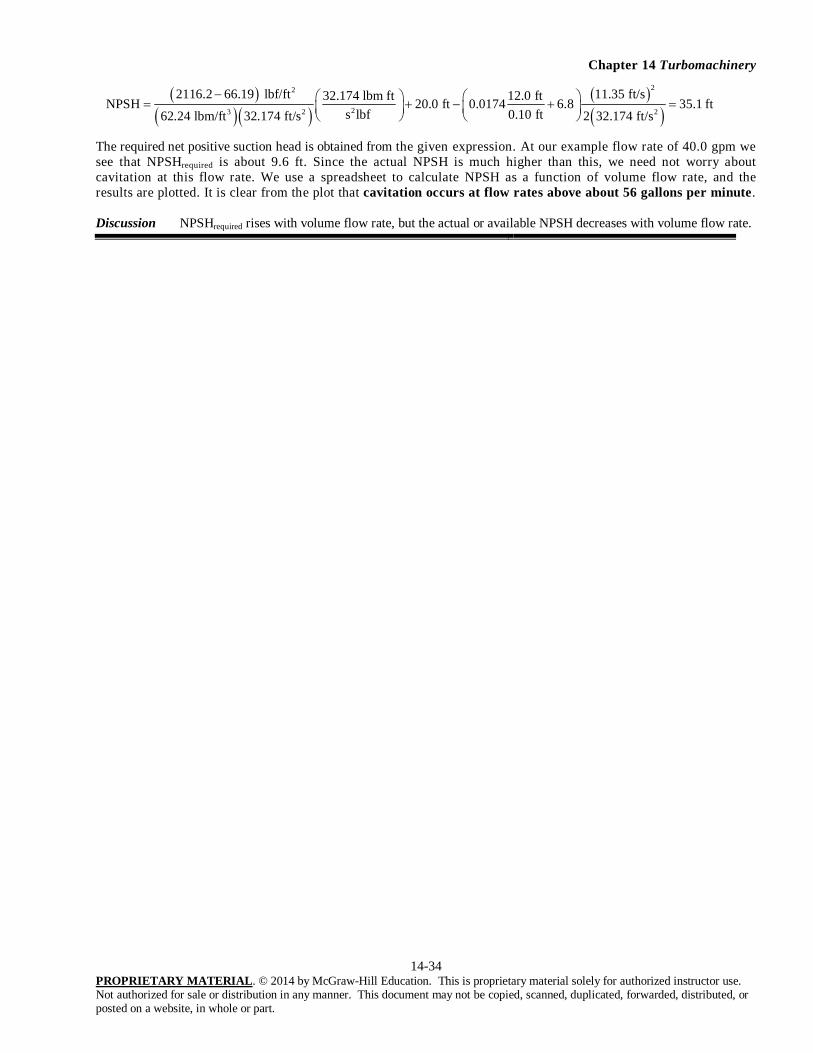
Chapter 14 Turbomachinery
14-34 PROPRIETARY MATERIAL. © 2014 by McGraw-Hill Education. This is proprietary material solely for authorized instructor use. Not authorized for sale or distribution in any manner. This document may not be copied, scanned, duplicated, forwarded, distributed, or posted on a website, in whole or part.
22
23 2 2
2116.2 66.19 lbf/ft 11.35 ft/s32.174 lbm ft 12.0 ftNPSH 20.0 ft 0.0174 6.8 35.1 ft0.10 fts lbf62.24 lbm/ft 32.174 ft/s 2 32.174 ft/s
The required net positive suction head is obtained from the given expression. At our example flow rate of 40.0 gpm we see that NPSHrequired is about 9.6 ft. Since the actual NPSH is much higher than this, we need not worry about cavitation at this flow rate. We use a spreadsheet to calculate NPSH as a function of volume flow rate, and the results are plotted. It is clear from the plot that cavitation occurs at flow rates above about 56 gallons per minute. Discussion NPSHrequired rises with volume flow rate, but the actual or available NPSH decreases with volume flow rate.

Chapter 14 Turbomachinery
14-35 PROPRIETARY MATERIAL. © 2014 by McGraw-Hill Education. This is proprietary material solely for authorized instructor use. Not authorized for sale or distribution in any manner. This document may not be copied, scanned, duplicated, forwarded, distributed, or posted on a website, in whole or part.
14-59E Solution We are to calculate the volume flow rate below which cavitation in a pump is avoided. Assumptions 1 The flow is steady. 2 The water is incompressible. Properties Patm = 14.696 psi = 2116.2 lbf/ft2. For water at T = 113oF, we interpolate in the property tables of the Appendix to get = 4.013 10-4 lbm/fts, = 61.82 lbm/ft3, and Pv = 201.9 lbf/ft2. Analysis The procedure is identical to that of the previous problem, except for the water properties. The calculations predict that the pump cavitates at volume flow rates greater than about 55 gpm. This is somewhat lower than the result of the previous problem, as expected, since cavitation occurs more readily in warmer water. Discussion Note that NPSHrequired does not depend on water temperature, but the actual or available NPSH decreases with temperature.

Chapter 14 Turbomachinery
14-36 PROPRIETARY MATERIAL. © 2014 by McGraw-Hill Education. This is proprietary material solely for authorized instructor use. Not authorized for sale or distribution in any manner. This document may not be copied, scanned, duplicated, forwarded, distributed, or posted on a website, in whole or part.
14-60 Solution For a given pump and piping system we are to estimate the maximum volume flow rate that can be pumped without cavitation. Assumptions 1 The flow is steady. 2 The water is incompressible. 3 The flow is turbulent. Properties Standard atmospheric pressure is Patm = 101.3 kPa. For water at T = 25oC, = 997.0 kg/m3, = 8.9110-4 kg/ms, and Pv = 3.169 kPa. Analysis We apply the steady energy equation in head form along a streamline from point 1 at the reservoir surface to point 2 at the pump inlet,
Energy equation: 2
1 1 1
2P Vg g
1 pump,uz h 2
2 2 22 turbine2
P Vz h
g g
, totalLh (1)
In Eq. 1 we have ignored the water speed at the reservoir surface (V1 0). There is no turbine in the piping system. Also, although there is a pump in the system, there is no pump between point 1 and point 2; hence the pump head term also drops out. We solve Eq. 1 for P2/(g), which is the pump inlet pressure expressed as a head,
Pump inlet pressure head: 2
atm2 2 21 2 ,total2 L
PP Vz z h
g g g
(2)
Note that in Eq. 2, we have recognized that P1 = Patm since the reservoir surface is exposed to atmospheric pressure. The available net positive suction head at the pump inlet is obtained from Eq. 14-8. After substitution of Eq. 2, and approximating 2 as 1.0, we get
Available NPSH: atm1 2 ,totalNPSH v
LP P
z z hg
(3)
Since we know Patm, Pv, and the elevation difference, all that remains is to estimate the total irreversible head loss through the piping system from the reservoir surface (1) to the pipe inlet (2), which depends on volume flow rate. Since the pipe diameter is constant, the total irreversible head loss is
2
,total 2L LL Vh f KD g
(4)
The rest of the problem is most easily solved on a computer. For a given volume flow rate, we calculate speed V and Reynolds number Re. From Re and the known pipe roughness, we use the Moody chart (or the Colebrook equation) to obtain friction factor f. The sum of all the minor loss coefficients is
0.85 0.3 1.15LK (5)
where we have not included the minor losses downstream of the pump, since they are irrelevant to the present analysis. We make one calculation by hand for illustrative purposes. At V& = 40.0 Lpm, the average speed of water through the pipe is
3
2 2
4 40.0 L/min4 1 m 1 min 1.474 m/s1000 L 60 s0.024 m
VA D
V V& & (6)
which produces a Reynolds number of Re = VD/ = 3.96 104. At this Reynolds number, and with roughness factor /D = 0, the Colebrook equation yields f = 0.0220. After substitution of the given variables, along with f, D, L, and Eqs. 4, 5, and 6 into Eq. 3, we calculate the available NPSH,
2
3
4
5
6
7
8
9
0 10 20 30 40 50 60 70
V& (Lpm)
NPSH (m)
Required NPSH
Available NPSH
No cavitation
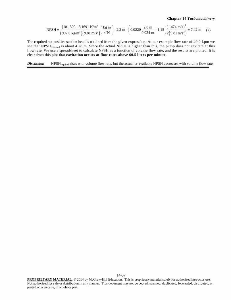
Chapter 14 Turbomachinery
14-37 PROPRIETARY MATERIAL. © 2014 by McGraw-Hill Education. This is proprietary material solely for authorized instructor use. Not authorized for sale or distribution in any manner. This document may not be copied, scanned, duplicated, forwarded, distributed, or posted on a website, in whole or part.
22
23 2 2
101,300 3,169 N/m 1.474 m/skg m 2.8 mNPSH 2.2 m 0.0220 1.15 7.42 m0.024 ms N997.0 kg/m 9.81 m/s 2 9.81 m/s
(7)
The required net positive suction head is obtained from the given expression. At our example flow rate of 40.0 Lpm we see that NPSHrequired is about 4.28 m. Since the actual NPSH is higher than this, the pump does not cavitate at this flow rate. We use a spreadsheet to calculate NPSH as a function of volume flow rate, and the results are plotted. It is clear from this plot that cavitation occurs at flow rates above 60.5 liters per minute. Discussion NPSHrequired rises with volume flow rate, but the actual or available NPSH decreases with volume flow rate.

Chapter 14 Turbomachinery
14-38 PROPRIETARY MATERIAL. © 2014 by McGraw-Hill Education. This is proprietary material solely for authorized instructor use. Not authorized for sale or distribution in any manner. This document may not be copied, scanned, duplicated, forwarded, distributed, or posted on a website, in whole or part.
14-61 Solution We are to calculate the volume flow rate below which cavitation in a pump is avoided, at two temperatures.
Assumptions 1 The flow is steady. 2 The water is incompressible.
Properties Standard atmospheric pressure is Patm = 101.3 kPa. For water at T = 80oC, = 971.9 kg/m3, = 3.5510-4 kg/ms, and Pv = 47.35 kPa. At T = 90oC, = 965.3 kg/m3, = 3.1510-4 kg/ms, and Pv = 70.11 kPa.
Analysis The procedure is identical to that of the previous problem, except for the water properties. The calculations predict that at T = 80oC, the pump cavitates at volume flow rates greater than 28.0 Lpm. This is substantially lower than the result of the previous problem, as expected, since cavitation occurs more readily in warmer water. At 90oC, the vapor pressure is very high since the water is near boiling (at atmospheric pressure, water boils at 100oC). For this case, the curves of NPSHavailable and NPSHrequired do not cross at all as seen in the plot, implying that the pump cavitates at any flow rate when T = 90oC.
Discussion Note that NPSHrequired does not depend on water temperature, but the actual or available NPSH decreases with temperature.
0
1
2
3
4
5
6
7
8
9
0 10 20 30 40 50 60 70
V& (Lpm)
NPSH(m)
Required NPSH
Available NPSH

Chapter 14 Turbomachinery
14-39 PROPRIETARY MATERIAL. © 2014 by McGraw-Hill Education. This is proprietary material solely for authorized instructor use. Not authorized for sale or distribution in any manner. This document may not be copied, scanned, duplicated, forwarded, distributed, or posted on a website, in whole or part.
14-62 Solution We are to calculate the volume flow rate below which cavitation in a pump is avoided, and compare with a previous case with a smaller pipe diameter.
Assumptions 1 The flow is steady. 2 The water is incompressible.
Properties Standard atmospheric pressure is Patm = 101.3 kPa. For water at T = 25oC, = 997.0 kg/m3, = 8.9110-4 kg/ms, and Pv = 3.169 kPa.
Analysis The analysis is identical to that of Problem 14-58, except that the pipe diameter is 48.0 mm instead of 24.0 mm. Compared to problem 14-58, at a given volume flow rate, the average speed through the pipe decreases by a factor of four since the pipe area increases by a factor of four. The Reynolds number goes down by a factor of two, but the flow is still turbulent (At our sample flow rate of 40.0 Lpm, Re = 1.98 104). For a smooth pipe at this Reynolds number, f = 0.0260. and the available NPSH is 7.81 m, slightly higher than the previous case with the smaller diameter pipe. After repeating the calculations at several flow rates, we find that the pump cavitates at V& = 65.5 Lpm. This represents an increase of about 8.3%. Cavitation occurs at a higher volume flow rate when the pipe diameter is increased because the irreversible head losses in the piping system upstream of the pump are decreased.
Discussion If a computer program like EES was used for Problem 14-58, it is a trivial matter to change the pipe diameter and re-do the calculations.

Chapter 14 Turbomachinery
14-40 PROPRIETARY MATERIAL. © 2014 by McGraw-Hill Education. This is proprietary material solely for authorized instructor use. Not authorized for sale or distribution in any manner. This document may not be copied, scanned, duplicated, forwarded, distributed, or posted on a website, in whole or part.
14-63E Solution We are to calculate the mass flow rate of slurry through a two-lobe rotary pump for given values of lobe volume and rotation rate. Assumptions 1 The flow is steady in the mean. 2 There are no leaks in the gaps between lobes or between lobes and the casing. 3 The slurry is incompressible. Analysis By studying the figure provided with this problem, we see that for each 360o rotation of the two counter-rotating shafts (n = 1 rotation), the total volume of pumped fluid is
Closed volume pumped per rotation: closed lobe4V V (1)
The volume flow rate is then calculated from Eq. 14-11,
gal/min 77.0rot 1
gal) 4(0.110)rot/min 175(n
n closedVV (2)
Thus, the volume flow rate is 77.0 gpm. Discussion If there were leaks in the pump, the volume flow rate would be lower. The fluid density was not used in the calculation of volume flow rate. However, the higher the density, the higher the required shaft torque and brake horsepower.
14-64E Solution We are to calculate the mass flow rate of slurry through a three-lobe rotary pump for given values of lobe volume and rotation rate. Assumptions 1 The flow is steady in the mean. 2 There are no leaks in the gaps between lobes or between lobes and the casing. 3 The slurry is incompressible. Analysis When there are three lobes, three lobe volumes are pumped for each 360o rotation of each rotor (n = 1 rotation). Thus, the total volume of pumped fluid is
Closed volume pumped per rotation: closed lobe6V V (1)
The volume flow rate is then calculated from Eq. 14-11,
gal/min 86.6 gal/min 63.86rot 1
gal) 6(0.0825)rot/min 175(n
n closedVV (2)
Thus, the volume flow rate is 86.6 gpm (to three significant digits). Discussion If there were leaks in the pump, the volume flow rate would be lower. This flow rate is slightly lower than that of the previous problem. Why? For the same overall diameter, it is clear from geometry that the more lobes, the less the volume per lobe, and the more “wasted” volume inside the pump – but the flow may be smoother (less unsteady) with more lobes.

Chapter 14 Turbomachinery
14-41 PROPRIETARY MATERIAL. © 2014 by McGraw-Hill Education. This is proprietary material solely for authorized instructor use. Not authorized for sale or distribution in any manner. This document may not be copied, scanned, duplicated, forwarded, distributed, or posted on a website, in whole or part.
14-65 Solution We are to calculate the volume flow rate of tomato paste through a positive-displacement pump for given values of lobe volume and rotation rate. Assumptions 1 The flow is steady in the mean. 2 There are no leaks in the gaps between lobes or between lobes and the casing. 3 The fluid is incompressible. Analysis By studying Fig. 14-27 or 14-30, we see that for each 360o rotation of the two counter-rotating shafts (n = 1 rotation), the total volume of pumped fluid is
Closed volume pumped per rotation: closed lobe4V V (1)
The volume flow rate is then calculated from Eq. 14-11,
3
3closed4 3.64 cm
336 rot/min 4892.2 cm /min1 rot
nn
& &VV 34890 cm /min (2)
Thus, the volume flow rate is 4890 cm3/min (to three significant digits). Discussion If there were leaks in the pump, the volume flow rate would be lower. The fluid density was not used in the calculation of volume flow rate. However, the higher the fluid density, the higher the required shaft torque and brake horsepower.
14-66 Solution We are to calculate the volume flow rate per rotation of a gear pump. Assumptions 1 The flow is steady in the mean. 2 There are no leaks in the gaps between lobes or between lobes and the casing. 3 The fluid is incompressible. Analysis From Fig. 14-26c, we count 14 teeth per gear. Thus, for each 360o rotation of each gear (n = 1 rotation), 14(0.350 cm3) of fluid is pumped. Sine there are two gears, the total volume of fluid pumped per rotation is 2(14)(0.350 cm3) = 9.80 cm3. Discussion The actual volume flow rate will be lower than this due to leakage in the gaps.

Chapter 14 Turbomachinery
14-42 PROPRIETARY MATERIAL. © 2014 by McGraw-Hill Education. This is proprietary material solely for authorized instructor use. Not authorized for sale or distribution in any manner. This document may not be copied, scanned, duplicated, forwarded, distributed, or posted on a website, in whole or part.
14-67 Solution We are to calculate the brake horsepower and net head of an idealized centrifugal pump at a given volume flow rate and rotation rate.
Assumptions 1 The flow is steady in the mean. 2 The water is incompressible. 3 The efficiency of the pump is 100% (no irreversible losses).
Properties We take the density of water to be = 998.0 kg/m3.
Analysis Since the volume flow rate (capacity) is given, we calculate the normal velocity components at the inlet and the outlet using Eq. 14-12,
Normal velocity, inlet:
3
1,n1 1
0.573 m /s 4.222 m/s2 2 0.120 m 0.180 m
Vr b
V&
V1 = V1,n, and V1,t = 0, since 1 = 0o. Similarly, V2,n = 2.3456 m/s and
Tangential component of absolute velocity at impeller outlet: o
2,t 2,n 2tan 2.3456 m/s tan(35 ) 1.6424 m/sV V
Now we use Eq. 14-17 to predict the net head,
2 2,t 1 1,tH r V r Vg
{
2
0
78.54 rad/s 0.240 m 1.6424 m/s 3.1558 m9.81 m/s
3.16 m
Finally, we use Eq. 14-16 to predict the required brake horsepower,
3
3 2 32
W s998. kg/m 9.81 m/s 0.573 m /s 3.1558 mkg m
bhp g H
17,700 W&V
Discussion The actual net head delivered to the water will be lower than this due to inefficiencies. Similarly, actual brake horsepower will be higher than that predicted here due to inefficiencies in the pump, friction on the shaft, etc.
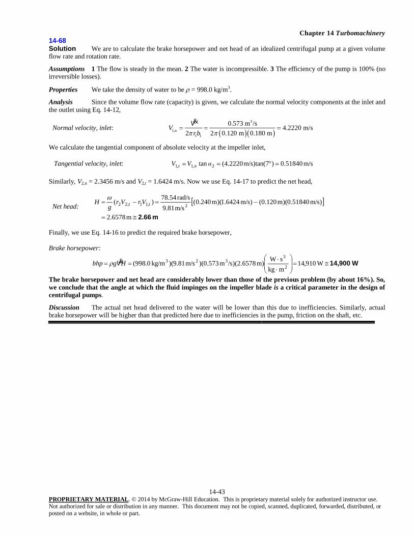
Chapter 14 Turbomachinery
14-43 PROPRIETARY MATERIAL. © 2014 by McGraw-Hill Education. This is proprietary material solely for authorized instructor use. Not authorized for sale or distribution in any manner. This document may not be copied, scanned, duplicated, forwarded, distributed, or posted on a website, in whole or part.
14-68 Solution We are to calculate the brake horsepower and net head of an idealized centrifugal pump at a given volume flow rate and rotation rate.
Assumptions 1 The flow is steady in the mean. 2 The water is incompressible. 3 The efficiency of the pump is 100% (no irreversible losses).
Properties We take the density of water to be = 998.0 kg/m3.
Analysis Since the volume flow rate (capacity) is given, we calculate the normal velocity components at the inlet and the outlet using Eq. 14-12,
Normal velocity, inlet:
3
1,n1 1
0.573 m /s 4.2220 m/s2 2 0.120 m 0.180 m
Vr b
&V
We calculate the tangential component of absolute velocity at the impeller inlet, Tangential velocity, inlet: m/s 0.51840)m/s)tan(7 (4.2220tan 2,1,1 αVV nt Similarly, V2,n = 2.3456 m/s and V2,t = 1.6424 m/s. Now we use Eq. 14-17 to predict the net head,
Net head:
m 2.66
m .65782
)m/s 0.51840)(m 0.120()m/s 6424.1)(m 0.240(m/s 9.81rad/s 78.54)( 2,11,22 tt VrVr
gH
Finally, we use Eq. 14-16 to predict the required brake horsepower, Brake horsepower:
W14,900
W910,14mkgsW)m 6578.2)(/sm 0.573)(m/s 81.9)(kg/m 0.998( 2
3323Hgbhp V
The brake horsepower and net head are considerably lower than those of the previous problem (by about 16%). So, we conclude that the angle at which the fluid impinges on the impeller blade is a critical parameter in the design of centrifugal pumps.
Discussion The actual net head delivered to the water will be lower than this due to inefficiencies. Similarly, actual brake horsepower will be higher than that predicted here due to inefficiencies in the pump, friction on the shaft, etc.

Chapter 14 Turbomachinery
14-44 PROPRIETARY MATERIAL. © 2014 by McGraw-Hill Education. This is proprietary material solely for authorized instructor use. Not authorized for sale or distribution in any manner. This document may not be copied, scanned, duplicated, forwarded, distributed, or posted on a website, in whole or part.
14-69 Solution We are to calculate the brake horsepower and net head of an idealized centrifugal pump at a given volume flow rate and rotation rate.
Assumptions 1 The flow is steady in the mean. 2 The water is incompressible. 3 The efficiency of the pump is 100% (no irreversible losses).
Properties We take the density of water to be = 998.0 kg/m3.
Analysis Since the volume flow rate (capacity) is given, we calculate the normal velocity components at the inlet and the outlet using Eq. 14-12,
Normal velocity, inlet:
3
1,n1 1
0.573 m /s 4.2220 m/s2 2 0.120 m 0.180 m
Vr b
&V
We calculate the tangential component of absolute velocity at the impeller inlet,
Tangential velocity, inlet: o1,t 1,n 2tan 4.2220 m/s tan( 10 ) 0.74446 m/sV V
Similarly, V2,n = 2.3456 m/s and V2,t = 1.6424 m/s. Now we use Eq. 14-17 to predict the net head,
Net head: 2 2,t 1 1,t 2
78.54 rad/s 0.240 m 1.6424 m/s 0.120 m 0.74446 m/s9.81 m/s
3.87104 m
H r V rVg
3.87 m
Finally, we use Eq. 14-16 to predict the required brake horsepower,
Brake horsepower: 3
3 2 32
W s998. kg/m 9.81 m/s 0.573 m /s 3.87104 mkg m
bhp g H
21,700 W&V
The brake horsepower and net head are considerably higher than those of the original problem (by about 23%). So, we conclude that the angle at which the fluid impinges on the impeller blade is a critical parameter in the design of centrifugal pumps. Here, reverse swirl has improved (increased the net head), but at the expense of higher bhp. So, a little reverse flow is desirable in terms of increasing the net head, but the increase in net head comes at a cost – more required power. Also, keep in mind that we are neglecting losses (assuming 100% efficiency). In real life, losses at the inlet may be significantly greater when the flow does not impinge parallel to the blades.
Discussion The actual net head delivered to the water will be lower than this due to inefficiencies. Similarly, actual brake horsepower will be higher than that predicted here due to inefficiencies in the pump, friction on the shaft, etc.

Chapter 14 Turbomachinery
14-45 PROPRIETARY MATERIAL. © 2014 by McGraw-Hill Education. This is proprietary material solely for authorized instructor use. Not authorized for sale or distribution in any manner. This document may not be copied, scanned, duplicated, forwarded, distributed, or posted on a website, in whole or part.
14-70 Solution For given flow conditions and stator blade shape at a given radius, we are to design the rotor blade. Specifically, we are to calculate the leading and trailing edge angles of the rotor blade and sketch its shape. We are also to decide how many rotor blades to construct. Assumptions 1 The air is nearly incompressible. 2 The flow area between hub and tip is constant. 3 Two-dimensional blade row analysis is appropriate. Analysis First we analyze flow through the stator from an absolute reference frame, using the two-dimensional approximation of a cascade (blade row) of stator blades as sketched in Fig. 1. Flow enters axially (horizontally), and is turned 26.6o downward. Since the axial component of velocity must remain constant to conserve mass, the magnitude of the velocity leaving the trailing edge of the stator, stV
r is calculated,
inst o
st
31.4 m/s 35.12 m/scos cos 26.6
VV
(1)
The direction of stVr
is assumed to be that of the stator trailing edge. In other words we assume that the flow turns nicely through the blade row and exits parallel to the trailing edge of the blade, as shown in the sketch. We convert stV
rto the relative reference frame moving with the rotor blades. At a radius of 0.50 m, the tangential
velocity of the rotor blades is
inVr
Stator blade row
stVr
26.6o
inVr
FIGURE 1 Analysis of the stator of a vaneaxial flow fan as a two-dimensional cascade of stator blades; absolute reference frame.
Rotor blade row
stVr
st, relativeVr
r
rl
Direction of rt, relativeV
r
rt
FIGURE 2 Analysis of the stator trailing edge velocity as it impinges on the rotor leading edge; relative reference frame.
rt inV Vr r
rt, relativeVr
r
rt
FIGURE 3 Analysis of the rotor trailing edge velocity; absolute reference frame.

Chapter 14 Turbomachinery
14-46 PROPRIETARY MATERIAL. © 2014 by McGraw-Hill Education. This is proprietary material solely for authorized instructor use. Not authorized for sale or distribution in any manner. This document may not be copied, scanned, duplicated, forwarded, distributed, or posted on a website, in whole or part.
2 rad 1 min1800 rot/min 0.50 m 94.25 m/srot 60 s
u r
(2)
Since the rotor blade row moves upward in the figure provided with this problem, we add a downward velocity with magnitude given by Eq. 2 to translate stV
r into the rotating reference frame sketched in Fig. 2. The angle of the leading edge
of the rotor, rl, can be calculated. After some trig,
o
oin strl
in
94.25 m/s 31.4 m/s tan 26.6tanarctan arctan 74.06
31.4 m/sr V
V
(3)
The air must now be turned by the rotor blade row in such a way that it leaves the trailing edge of the rotor blade at zero angle (axially – no swirl) from an absolute reference frame. This determines the rotor’s trailing edge angle, rt. Specifically, when we add an upward velocity of magnitude r (Eq. 2) to the relative velocity exiting the trailing edge of the rotor, rt, relativeV
r, we convert back to the absolute reference frame, and obtain rtV
r, the velocity leaving the rotor trailing
edge. It is this velocity, rtVr
, which must be axial (horizontal). Furthermore, to conserve mass rtVr
must equal inVr
since we
are assuming incompressible flow. Working “backwards” we construct rt, relativeVr
in Fig. 3. Some trigonometry reveals that
ort
in
94.25 m/sarctan arctan 71.5731.4 m/s
rV
(4)
We conclude that the rotor blade at this radius has a leading edge angle of about 74.1o (Eq. 3) and a trailing edge angle of about 71.6o (Eq. 4). A sketch of the rotor blade is provided in Fig. 2; it is clear that the blade is nearly straight, at least at this radius. Finally, to avoid interaction of the stator blade wakes with the rotor blade leading edges, we choose the number of rotor blades such that it has no common denominator with the number of stator blades. Since there are 18 stator blades, we pick a number like 13, 17, or 19 rotor blades. 16 would not be appropriate since it shares a common denominator of 2 with the number 18. Discussion We can easily repeat the calculation for all radii from hub to tip, completing the design of the entire rotor.

Chapter 14 Turbomachinery
14-47 PROPRIETARY MATERIAL. © 2014 by McGraw-Hill Education. This is proprietary material solely for authorized instructor use. Not authorized for sale or distribution in any manner. This document may not be copied, scanned, duplicated, forwarded, distributed, or posted on a website, in whole or part.
14-71 Solution We are to calculate the combined shutoff head and free delivery for two pumps in series, and discuss why the weaker pump should be shut off and bypassed above some flow rate.
Assumptions 1 The water is incompressible. 2 The flow is steady.
Analysis The pump performance curves for both pumps individually and for their combination in series are plotted here. At zero flow rate, the shutoff head of the two pumps in series is equal to the sum of their individual shutoff heads: H0,combined = H0,1 + H0,2 = 6.33 m + 9.25 m. Thus the combined shutoff head is 15.6 m (to three significant digits). At free delivery conditions (zero net head), the free delivery of the two pumps in series is limited to that of the stronger pump, in this case Pump 2: max,combinedV& = MAX( max,1V& , max,2V& ) = 13.999 Lpm. Thus the combined free delivery is 14.0 Lpm (to three significant digits). As volume flow rate increases, the combined net pump head is equal to the sum of the net pump heads of the individual pumps, as seen on the plot. However, the free delivery of Pump 1 is
2 00 max 2
6.33 m0 10.0 Lpm0.0633 m/(Lpm)
HH aa
& &V V
Above this flow rate, Pump 1 no longer contributes to the flow. In fact, it becomes a liability to the system since its net head would be negative at flow rates above 10.0 Lpm. For this reason, it is wise to shut off and bypass Pump 1 above 10.0 Lpm. We are assuming no additional losses in the bypass line around pump 1.
Discussion The free delivery of Pump 2 is 14.0 Lpm. The free delivery of the two-pump system is no better than that of Pump 2 alone, since Pump 1 is shut off and bypassed at flow rates above 10.0 Lpm.
14-72 Solution We are to calculate the free delivery and shutoff head for two pumps in parallel, and discuss why the weaker pump should be shut off and bypassed above some net head.
Assumptions 1 The water is incompressible. 2 The flow is steady. Analysis The pump performance curves for both pumps and for their combination in parallel are plotted. At zero flow rate, the shutoff head of the two pumps in parallel is equal to that of the stronger pump, in this case Pump 2: H0,combined = MAX(H0,1, H0,2) = 9.25 m. Thus the combined shutoff head is 9.25 m. At free delivery conditions (zero net head), the free delivery of the two pumps in parallel is the sum of their individual free deliveries: max,combinedV& = max,1V& + max,2V& = 10.0 Lpm + 14.0 Lpm. Thus the combined free delivery is 24.0 Lpm. As net head increases, the combined capacity is equal to the sum of the capacities of the individual pumps, as seen in the plot. However, the shutoff head of Pump 1 (6.33 m) is lower than that of Pump 2 (9.25 m). Above the shutoff head of Pump 1, that pump no longer contributes to the flow. In fact, it becomes a liability to the system since it cannot sustain such a high head. If not shut off and blocked, the volume flow rate through Pump 1 would be negative at net heads above 6.33 m. For this reason, it is wise to shut off and block Pump 1 above 6.33 m.
Discussion The shutoff head of Pump 2 is 9.25 m. The shutoff head of the two-pump system is no better than that of Pump 2 alone, since Pump 1 is shut off and blocked at net heads above 9.25 m.
0
2
4
6
8
10
12
14
16
0 5 10 15
LpmV&
H (m)
Combined net head
Pump 1
Pump 2
Bypass Pump 1
0
1
2
3
4
5
6
7
8
9
10
0 5 10 15 20 25
LpmV&
H (m) Combined
capacity
Pump 1
Pump 2
Block Pump 1
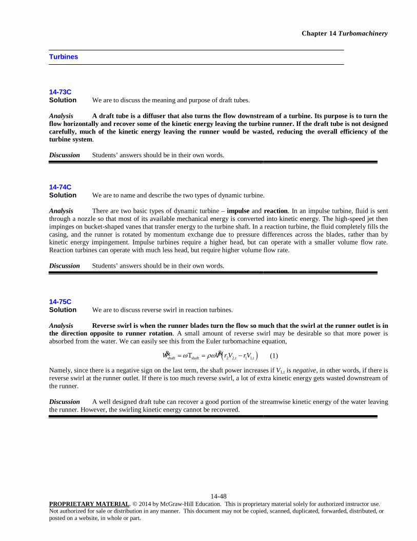
Chapter 14 Turbomachinery
14-48 PROPRIETARY MATERIAL. © 2014 by McGraw-Hill Education. This is proprietary material solely for authorized instructor use. Not authorized for sale or distribution in any manner. This document may not be copied, scanned, duplicated, forwarded, distributed, or posted on a website, in whole or part.
Turbines
14-73C Solution We are to discuss the meaning and purpose of draft tubes. Analysis A draft tube is a diffuser that also turns the flow downstream of a turbine. Its purpose is to turn the flow horizontally and recover some of the kinetic energy leaving the turbine runner. If the draft tube is not designed carefully, much of the kinetic energy leaving the runner would be wasted, reducing the overall efficiency of the turbine system. Discussion Students’ answers should be in their own words.
14-74C Solution We are to name and describe the two types of dynamic turbine. Analysis There are two basic types of dynamic turbine – impulse and reaction. In an impulse turbine, fluid is sent through a nozzle so that most of its available mechanical energy is converted into kinetic energy. The high-speed jet then impinges on bucket-shaped vanes that transfer energy to the turbine shaft. In a reaction turbine, the fluid completely fills the casing, and the runner is rotated by momentum exchange due to pressure differences across the blades, rather than by kinetic energy impingement. Impulse turbines require a higher head, but can operate with a smaller volume flow rate. Reaction turbines can operate with much less head, but require higher volume flow rate. Discussion Students’ answers should be in their own words.
14-75C Solution We are to discuss reverse swirl in reaction turbines. Analysis Reverse swirl is when the runner blades turn the flow so much that the swirl at the runner outlet is in the direction opposite to runner rotation. A small amount of reverse swirl may be desirable so that more power is absorbed from the water. We can easily see this from the Euler turbomachine equation,
shaft shaft 2 2,t 1 1,tTW r V rV V&& (1)
Namely, since there is a negative sign on the last term, the shaft power increases if V1,t is negative, in other words, if there is reverse swirl at the runner outlet. If there is too much reverse swirl, a lot of extra kinetic energy gets wasted downstream of the runner. Discussion A well designed draft tube can recover a good portion of the streamwise kinetic energy of the water leaving the runner. However, the swirling kinetic energy cannot be recovered.

Chapter 14 Turbomachinery
14-49 PROPRIETARY MATERIAL. © 2014 by McGraw-Hill Education. This is proprietary material solely for authorized instructor use. Not authorized for sale or distribution in any manner. This document may not be copied, scanned, duplicated, forwarded, distributed, or posted on a website, in whole or part.
14-76C Solution We are to discuss why turbines have higher efficiencies than pumps. Analysis There are several reasons for this. First, pumps normally operate at higher rotational speeds than do turbines; therefore, shear stresses and frictional losses are higher. Second, conversion of kinetic energy into flow energy (pumps) has inherently higher losses than does the reverse (turbines). You can think of it this way: Since pressure rises across a pump (adverse pressure gradient), but drops across a turbine (favorable pressure gradient), boundary layers are less likely to separate in a turbine than in a pump. Third, turbines (especially hydroturbines) are often much larger than pumps, and viscous losses become less important as size increases. Finally, while pumps often operate over a wide range of flow rates, most electricity-generating turbines run within a narrower operating range and at a controlled constant speed; they can therefore be designed to operate very efficiently at those conditions. Discussion Students’ answers should be in their own words.
14-77C Solution We are to discuss the classification of dynamic pumps and reaction turbines. Analysis Dynamic pumps are classified according to the angle at which the flow exits the impeller blade – centrifugal, mixed-flow, or axial. Reaction turbines, on the other hand, are classified according to the angle that the flow enters the runner – radial, mixed-flow, or axial. This is the main difference between how dynamic pumps and reaction turbines are classified. Discussion Students’ answers should be in their own words.
14-78 Solution We are to estimate the power production from a hydroelectric plant.
Properties The density of water at T = 25oC is 997.0 kg/m3.
Analysis The ideal power produced by one hydroturbine is
ideal gross
3 2 32 6
N W 1 MW 997.0 kg/m 9.807 m/s 13.6 m /s 284 m 37.765 MWN m/skg m/s 10 W
W g H
&& V
But inefficiencies in the turbine, the generator, and the rest of the system reduce the actual electrical power output. For each turbine,
electrical ideal turbine generator other 37.765 MW 0.959 0.942 0.956 32.615 MWW W & &
Finally, since there are 14 turbines in parallel, the total power produced is
total, electrical electrical14 14 32.615 MW 456.61 MWW W 457 MW& &
Discussion A small improvement in any of the efficiencies ends up increasing the power output, and increases the power company’s profitability.

Chapter 14 Turbomachinery
14-50 PROPRIETARY MATERIAL. © 2014 by McGraw-Hill Education. This is proprietary material solely for authorized instructor use. Not authorized for sale or distribution in any manner. This document may not be copied, scanned, duplicated, forwarded, distributed, or posted on a website, in whole or part.
14-79 Solution We are to calculate several performance parameters for a Pelton wheel turbine. Assumptions 1 Frictional losses are negligible, so that the Euler turbomachine equation applies, and the relative exit speed of the jet is the same as its relative inlet speed. 2 The turning angle is sufficient to prevent the exiting fluid from striking the next bucket. 3 The water is at 20oC. Properties The density of water at T = 20oC is 998.0 kg/m3. Analysis (a) The volume flow rate of the jet is equal to jet area times jet velocity,
22 / 4 102 m/s 0.100 m / 4j jV D 30.801 m /sV&
(b) The maximum output shaft power occurs when the bucket moves at half the jet speed (r = Vj/2). Thus,
102 m/s 27.87 rad/s2 2 1.83 m
rot 60 s 27.87 rad/s2 rad min
jVr
n
266 rpm&
(c) The ideal shaft power is found from Eq. 14-40,
ideal
33 o
2
6
1 cos
rad m 102 m/s 998.0 kg/m 27.87 1.83 m 0.801 1 cos165s s 2
N s W s 1 MW 4.09 MWkg m N m 10 W
jW r V r
V&&
where we have substituted r = Vj/2 for convenience in the calculations. Since the turbine efficiency is given, we calculate the actual output shaft power, or brake horsepower,
actual ideal turbine 4.09 MW 0.82W bhp W 3.35 MW& &
Discussion At other rotation speeds, the turbine would not be as efficient.
14-80 Solution We are to estimate the ideal power production from a hydroturbine. Assumptions 1 Frictional losses are negligible. 2 The water is at 20oC. Properties The density of water at T = 20oC is 998.0 kg/m3. Analysis The ideal power produced by a hydroturbine is
MW 3.16
W10
MW 1mNsW
mkgsN)m 340)(/sm 0.95)(m/s 81.9)(kg/m 0.998( 6
2323
grossideal HgW V
Discussion If a hydroelectric dam were to be built on this site, the actual power output per turbine would be smaller than this, of course, due to inefficiencies.

Chapter 14 Turbomachinery
14-51 PROPRIETARY MATERIAL. © 2014 by McGraw-Hill Education. This is proprietary material solely for authorized instructor use. Not authorized for sale or distribution in any manner. This document may not be copied, scanned, duplicated, forwarded, distributed, or posted on a website, in whole or part.
14-81 Solution We are to prove that the maximum power of a Pelton wheel occurs when r = Vj/2 (bucket moving at half the jet speed). Assumptions 1 Frictional losses are negligible, so that the Euler turbomachine equation applies, and the relative exit speed of the jet is the same as its relative inlet speed. 2 The turning angle is sufficient to prevent the exiting fluid from striking the next bucket. 3 The fluid, jet speed, volume flow rate, turning angle, and wheel radius are fixed – rotation rate is the only variable about which we are concerned. Analysis With the stated assumptions, Eq. 14-40 applies, namely,
Output shaft power: shaft 1 cosjW r V r V&& (1)
We differentiate Eq. 1 with respect to , and set the derivative equal to zero,
Maximum power:
2shaft 0 0 2 0j jdW d V r V r
d d
& (2)
Solution of Eq. 2 yields the desired result, namely, the maximum power of a Pelton wheel occurs when r = Vj/2 (bucket moving at half the jet speed). Discussion To be sure that we have not identified a minimum instead of a maximum, we could substitute some numerical values and plot shaftW& versus . It turns out that we have indeed found the maximum value of shaftW& .

Chapter 14 Turbomachinery
14-52 PROPRIETARY MATERIAL. © 2014 by McGraw-Hill Education. This is proprietary material solely for authorized instructor use. Not authorized for sale or distribution in any manner. This document may not be copied, scanned, duplicated, forwarded, distributed, or posted on a website, in whole or part.
14-82 Solution We are to estimate the power generated by a wind turbine. Assumptions 1 The power coefficient is 0.42 and the combined gearbox/generator efficiency is 0.88. Properties The air density is given as 1.204 kg/m3. Analysis (a) From the definition of power coefficient,
3 3 21 1rotor shaft output 2 2 / 4P PW C V A C V D &
But the actual electrical power produced is lower than this because of generator inefficiencies,
kW 168
W930,167
m/sNW
m/skgN
8m) (45m/s) 8.7)(kg/m 204.1()42.0()88.0(
8
2
233
23
neratorgearbox/geoutput electrical
DVCW p
(b) If we could achieve the Betz limit, the shaft power output would increase by a factor of CP, Betz/CP, real. Assuming the same gearbox/generator efficiency,
kW 237
W938,236
m/sNW
m/skgN
8
m) (45m/s) 8.7)(kg/m 204.1(2716
)88.0(
8
2
233
23Betz,
neratorgearbox/geidealoutput electrical
DVCW p
Discussion We give the final answers to three significant digits since we cannot expect any better than that. The Betz limit is unachievable in practice, so the solution of Part (b) is academic.

Chapter 14 Turbomachinery
14-53 PROPRIETARY MATERIAL. © 2014 by McGraw-Hill Education. This is proprietary material solely for authorized instructor use. Not authorized for sale or distribution in any manner. This document may not be copied, scanned, duplicated, forwarded, distributed, or posted on a website, in whole or part.
14-83 Solution We are to calculate runner blade angles, required net head, and power output for a Francis turbine. Assumptions 1 The flow is steady. 2 The fluid is water at 20oC. 3 The blades are infinitesimally thin. 4 The flow is everywhere tangent to the runner blades. 5 We neglect irreversible losses through the turbine. Properties For water at 20oC, = 998.0 kg/m3. Analysis We solve for the normal component of velocity at the inlet,
3
2,n2 2
340 m /s 37.0 m/s2 2 2.00 m 0.731 m
Vr b
V& (1)
Using the figure provided with this problem as a guide, the tangential velocity component at the inlet is
o2,t 2,n 2tan 37.0 m/s tan30 21.4 m/sV V (2)
The angular velocity is = 2 n&/60 = 18.85 rad/s. The tangential velocity component of the absolute velocity at the inlet is obtained from trigonometry to be (see Eq.
14-45)
2,n2,t 2
2tanV
V r
From the above relationship, we solve for the runner leading edge angle 2,
2,n2
2 2,t
37.0 m/sarctan arctan18.85 rad/s 2.00 m 21.4 m/s
Vr V
o66.2 (3)
Equations 1 through 3 are repeated for the runner outlet, with the following results:
Runner outlet: 1,n 1,t 117.3 m/s, 3.05 m/s, V V o36.1 (4)
Using Eqs. 2 and 4, the shaft output power is estimated from the Euler turbomachine equation,
3 3
shaft 2 2,t 1 1,t
2 38
3 6 2
998.0 kg/m 18.85 rad/s 340 m /s 2.00 m 21.4 m/s 1.42 m 3.05 m/s
kg m MW s 2.46 10 246.055 MWs 10 kg m
W r V rV
246 MW
V&&
(5)
Finally, we calculate the required net head using Eq. 14-44, assuming that turbine = 100% since we are ignoring irreversibilities,
6 2
33 2 3
246.055 MW 10 kg mMW s998.0 kg/m 9.81 m/s 340 m /s
bhpHg
73.9 mV&
(6)
Since the required net head is less than the gross net head, the design is feasible. Discussion This is a preliminary design in which we are neglecting irreversibilities. Actual output power will be lower, and actual required net head will be higher than the values predicted here.

Chapter 14 Turbomachinery
14-54 PROPRIETARY MATERIAL. © 2014 by McGraw-Hill Education. This is proprietary material solely for authorized instructor use. Not authorized for sale or distribution in any manner. This document may not be copied, scanned, duplicated, forwarded, distributed, or posted on a website, in whole or part.
14-84 Solution We are to examine the effect of runner outlet angle 1 on the required net head and the output power of a hydroturbine. Assumptions 1 The flow is steady. 2 The fluid is water at 20oC. 3 The blades are infinitesimally thin. 4 The flow is everywhere tangent to the runner blades. 5 We neglect irreversible losses through the turbine. Properties For water at 20oC, = 998.0 kg/m3. Analysis We repeat the calculations of the previous problem, but with 1 varying from -20o to 20o. The results are plotted. We see that the required net head H and the output brake horsepower bhp decrease as 1 increases. This agrees with our expectations, based on the negative sign on the V1,t term in the Euler turbomachine equation. In other words, we can produce greater power by increasing the reverse swirl, but at the cost of increased required net head. However, when 1 is smaller than about -9o, the required net head rises above Hgross, which is impossible, even with no irreversibilities. Thus, when 1 < -9o, the predicted net head and brake horsepower are not feasible – they violate the second law of thermodynamics.
Discussion A small amount of reverse swirl is usually good, but too much reverse swirl is not good.
0
20
40
60
80
100
-20 -10 0 10 200
100
200
300
400
500
600
700
1 (degrees)
bhp (MW) H (m)
bhp
H
Hgross
Chapter 14 Turbomachinery
14-55 PROPRIETARY MATERIAL. © 2014 by McGraw-Hill Education. This is proprietary material solely for authorized instructor use. Not authorized for sale or distribution in any manner. This document may not be copied, scanned, duplicated, forwarded, distributed, or posted on a website, in whole or part.
14-85 Solution We are to calculate flow angles, required net head, and power output for a Francis turbine. Assumptions 1 The flow is steady. 2 The fluid is water at 20oC. 3 The blades are infinitesimally thin. 4 The flow is everywhere tangent to the runner blades. 5 We neglect irreversible losses through the turbine. Properties For water at 20oC, = 998.0 kg/m3. Analysis The angular velocity is = 2 n&/60 = 16.7552 rad/s. We solve for the normal component of velocity at the inlet,
3
2,n2 2
80.0 m /s 7.4896 m/s2 2 2.00 m 0.85 m
Vr b
&V (1)
The tangential velocity component of the absolute velocity at the inlet is obtained from trigonometry to be (see Eq. 14-45)
m/s 990.3071.4tan
m/s 7.4896m) 00.2)(rad/s 7552.16(tan 2
,22,2
n
tV
rV (2)
From these two components of V2 in the absolute coordinate system, we calculate the angle 2 through which the wicket gates should turn the flow,
76.4413.76m/s 7.4896m/s 30.990tantan 1
,2
,212
n
t
VV
(3)
In exactly similar fashion, we solve for the velocity components and swirl angle at the runner outlet. We get Runner outlet: V1,n = 4.6639 m/s, V1,t = 4.7334 m/s, 1 = 45.4 (4) Using the tangential velocity components of Eqs. 2 and 4, the shaft output power is estimated from the Euler turbomachine equation,
MW 73.8
MW 73.775mkg 10sMW
smkg 107.3775
m/s) m)(4.7334 30.1()m/s 30.990 )(m 2.00 (/s)m 0rad/s)(80. 7552.16)(kg/m 0.998(
)(
26
3
3
27
33
,11,22shaft tt VrVrW V
(5)
Finally, we calculate the required net head using Eq. 14-44, assuming that turbine = 100% since we are ignoring irreversibilities,
m 94.2
m 194.94
sMWmkg 10
/s)m )(80.0m/s 81.9)(kg/m 0.998(MW 73.775
3
26
323VgbhpH
(6)
Discussion This is a preliminary design in which we are neglecting irreversibilities. Actual output power will be lower, and actual required net head will be higher than the values predicted here. Notice the double negative in the outlet terms of Eq. 5 – reverse swirl leads to greater performance, but requires more head.

Chapter 14 Turbomachinery
14-56 PROPRIETARY MATERIAL. © 2014 by McGraw-Hill Education. This is proprietary material solely for authorized instructor use. Not authorized for sale or distribution in any manner. This document may not be copied, scanned, duplicated, forwarded, distributed, or posted on a website, in whole or part.
14-86E Solution We are to calculate flow angles, required net head, and power output for a Francis turbine. Assumptions 1 The flow is steady. 2 The fluid is water at 68oF. 3 The blades are infinitesimally thin. 4 The flow is everywhere tangent to the runner blades. 5 We neglect irreversible losses through the turbine. Properties For water at 68oF, = 62.32 lbm/ft3. Analysis The angular velocity is = 2 n&/60 = 12.57 rad/s. The volume flow rate is (4.70 106 gpm)[ft3/s / (448.83 gpm)] = 10,470 ft3/s. We solve for the normal component of velocity at the inlet,
3
2,n2 2
10, 470 ft /s 97.1 ft/s2 2 6.60 ft 2.60 ft
Vr b
V&
(1)
The tangential velocity component of the absolute velocity at the inlet is obtained from trigonometry to be (see Eq. 14-45)
2,n2,t 2 o
2
97.12 ft/s12.57 rad/s 6.60 ft 69.3 ft/stan tan 82V
V r
(2)
From these two components of V2 in the absolute coordinate system, we calculate the angle 2 through which the wicket gates should turn the flow,
2,t1 12
2,n
69.3 ft/stan tan97.1 ft/s
VV
o35.5 (3)
In exactly similar fashion, we solve for the velocity components and swirl angle at the runner outlet. We get
Runner outlet: 1,n 1,t 152.6 ft/s, 4.49 ft/s, V V o4.9 (4)
Since 1 is positive, this turbine operates with a small amount of forward swirl. Using the tangential velocity components of Eqs. 2 and 4, the shaft output power is estimated from the Euler turbomachine equation,
3 3shaft 2 2,t 1 1,t
2
38
62.32 lbm/ft 12.57 rad/s 10, 470 ft /s
lbf s 6.60 ft 69.3 ft/s 4.40 ft 4.49 ft/s32.174 lbm ft
ft lbf 1.8182 10 hp s 1.116 10s ft lbf
W r V rV
52.03 10 hp
V&&
(5)
Finally, we calculate the required net head using Eq. 14-44, assuming that turbine = 100% since we are ignoring irreversibilities,
8
23 2 3
1.116 10 ft lbf/s 32.174 lbm ftlbf s62.32 lbm/ft 32.174 ft/s 10, 470 ft /s
bhpHg
171 ft
V& (6)
Discussion This is a preliminary design in which we are neglecting irreversibilities. Actual output power will be lower, and actual required net head will be higher than the values predicted here.
Chapter 14 Turbomachinery
14-57 PROPRIETARY MATERIAL. © 2014 by McGraw-Hill Education. This is proprietary material solely for authorized instructor use. Not authorized for sale or distribution in any manner. This document may not be copied, scanned, duplicated, forwarded, distributed, or posted on a website, in whole or part.
14-87E Solution We are to calculate the runner blade trailing edge angle such that there is no swirl. At this value of 1, we are to also calculate the shaft power.
Assumptions 1 The flow is steady. 2 The fluid is water at 68oF. 3 The blades are infinitesimally thin. 4 The flow is everywhere tangent to the runner blades. 5 We neglect irreversible losses through the turbine.
Properties For water at 68oF, = 62.32 lbm/ft3.
Analysis Using EES or other software, we adjust 1 by trial and error until 1 = 0. It turns out that 1 = 43.6o, at which shaftW& = 2.12 105 hp.
Discussion It turns out that the swirl angle at the runner output is a strong function of 1 – a small change in 1 leads to a large change in 1. The shaft power increases, as expected, since the original swirl angle was positive. The increase in shaft power is less than 5%.

Chapter 14 Turbomachinery
14-58 PROPRIETARY MATERIAL. © 2014 by McGraw-Hill Education. This is proprietary material solely for authorized instructor use. Not authorized for sale or distribution in any manner. This document may not be copied, scanned, duplicated, forwarded, distributed, or posted on a website, in whole or part.
14-88 Solution For given flow conditions and stator blade shape at a given radius, we are to design the rotor vane (bucket) for a single-stage turbine. Specifically, we are to calculate the leading and trailing edge angles of the rotor blade and sketch its shape. Assumptions 1 The water is nearly incompressible. 2 The flow area between hub and tip is constant. 3 Two-dimensional blade row analysis is appropriate. Analysis First we analyze flow through the stator from an absolute reference frame, using the two-dimensional approximation of a cascade (blade row) of stator blades as sketched in Fig. 1. Flow enters axially (horizontally), and is turned 50.3o upward. Since the axial component of velocity must remain constant to conserve mass, the magnitude of the velocity leaving the trailing edge of the stator, stV
r is
calculated,
inst o
st
8.31 m/s 13.009 m/scos cos 50.3
VV
(1)
The direction of stVr
is assumed to be that of the stator trailing edge. In other words we assume that the flow turns nicely through the blade row and exits parallel to the trailing edge of the blade, as shown in the sketch.
We convert stV
rto the relative reference frame moving with the rotor vanes. At a radius of 0.324 m, the tangential
velocity of the rotor vanes is
inVr
Stator blade row
stVr
50.3o
inVr
FIGURE 1 Analysis of the stator of an axial turbine as a two-dimensional cascade of stator blades; absolute reference frame.
Rotor vane row
stVr
st, relativeVr
r
rl
rt, relativeVr
rt
inVr
FIGURE 2 Analysis of the stator trailing edge velocity as it impinges on the rotor leading edge; relative reference frame.
rt inV Vr r
rt, relativeVr
r
rt
FIGURE 3 Analysis of the rotor trailing edge velocity; absolute reference frame.

Chapter 14 Turbomachinery
14-59 PROPRIETARY MATERIAL. © 2014 by McGraw-Hill Education. This is proprietary material solely for authorized instructor use. Not authorized for sale or distribution in any manner. This document may not be copied, scanned, duplicated, forwarded, distributed, or posted on a website, in whole or part.
2 rad 1 min360 rot/min 0.324 m 12.215 m/srot 60 s
u r
(2)
Since the rotor blade row moves upward in the figure provided with this problem, we add a downward velocity with magnitude given by Eq. 2 to translate stV
r into the rotating reference frame sketched in Fig. 2. The angle of the leading edge
of the rotor, rl, can be calculated. After some trig,
o
oin strl
in
12.215 m/s 8.31 m/s tan 50.3tanarctan arctan 14.86
8.31 m/sr V
V
(3)
The water must now be turned by the rotor vane row in such a way that it leaves the trailing edge of the rotor vane at zero angle (axially – no swirl) from an absolute reference frame. This determines the rotor’s trailing edge angle, rt. Specifically, when we add an upward velocity of magnitude r (Eq. 2) to the relative velocity exiting the trailing edge of the rotor, rt, relativeV
r, we convert back to the absolute reference frame, and obtain rtV
r, the velocity leaving the rotor trailing
edge. It is this velocity, rtVr
, which must be axial (horizontal). Furthermore, to conserve mass rtVr
must equal inVr
since we
are assuming incompressible flow. Working “backwards” we construct rt, relativeVr
in Fig. 3. Some trigonometry reveals that
ort
in
12.215 m/sarctan arctan 55.778.31 m/s
rV
(4)
We conclude that the rotor blade at this radius has a leading edge angle of about 14.9o (Eq. 3) and a trailing edge angle of about 55.8o (Eq. 4). A sketch of the rotor vane is provided in Fig. 2; the vane is curved to turn the flow. Some turbine vanes are turned a lot more than this, hence the name “bucket”. Finally, to avoid interaction of the stator blade wakes with the rotor vane leading edges, we choose the number of rotor vanes such that it has no common denominator with the number of stator blades. Since there are 16 stator blades, we pick a number like 13, 15, or 17 rotor vanes. 14 or 18 would not be appropriate since they share a common denominator of 2 with the number 16.
Discussion We can easily repeat the calculation for all radii from hub to tip, completing the design of the entire rotor.

Chapter 14 Turbomachinery
14-60 PROPRIETARY MATERIAL. © 2014 by McGraw-Hill Education. This is proprietary material solely for authorized instructor use. Not authorized for sale or distribution in any manner. This document may not be copied, scanned, duplicated, forwarded, distributed, or posted on a website, in whole or part.
14-89 Solution We are to prove that a = 1/3 for maximum wind turbine efficiency.
Analysis From the wind turbine section, the power coefficient, which can also be thought of as an efficiency, is
2rotor shaft output31
12
4 1P
WC a a
V A
&
To find the maximum (or minimum), we take the derivative of CP and set dCP/da = 0,
2 3 24 2 4 1 4 3PP
dCC a a a a ada
So, dCP/da = 0 when
23 4 1 0a a
We solve using the quadratic rule, yielding
4 16 12 / 6 1 or 1/ 3a
It turns out that a = 1 yields CP = 0, which is a minimum. The maximum is when a = 1/3, and yields CP = 16/27.
Discussion This is the famous Betz limit for wind turbines. No real wind turbine can outperform this limit.
14-90E Solution We are to estimate the power production from a hydroelectric plant. Properties The density of water at T = 50oF is 62.41 lbm/ft3. Analysis The ideal power produced by one hydroturbine is
ideal gross
2 33 2
6
lbf s ft 1.356 W 1 min 1 MW 62.41 lbm/ft 32.2 ft/s 189,400 gal/min 859 ft 0.133732.2 lbm ft gal ft lbf/s 60 s 10 W
30.681 MW
W g H
&& V
But inefficiencies in the turbine, the generator, and the rest of the system reduce the actual electrical power output. For each turbine,
electrical ideal turbine generator other 30.681 MW 0.963 0.939 1 0.036 26.745 MWW W & &
Finally, since there are 10 turbines in parallel, the total power produced is
total, electrical electrical10 10 26.745 MW 267.45 MWW W 267 MW& &
Discussion A small improvement in any of the efficiencies ends up increasing the power output, and increases the power company’s profitability.

Chapter 14 Turbomachinery
14-61 PROPRIETARY MATERIAL. © 2014 by McGraw-Hill Education. This is proprietary material solely for authorized instructor use. Not authorized for sale or distribution in any manner. This document may not be copied, scanned, duplicated, forwarded, distributed, or posted on a website, in whole or part.
14-91 Solution We are to estimate the required disk diameter of a wind turbine and how many homes a wind farm can serve. Assumptions 1 The power coefficient is 0.41 and the combined gearbox/generator efficiency is 0.928. The power distribution system has an efficiency of 96%. Properties The air density is given as 1.2 kg/m3. Analysis (a) From the definition of power coefficient,
3 3 21 1rotor shaft output 2 2 / 4P PW C V A C V D &
But the actual electrical power produced is lower than this because of gearbox and generator inefficiencies, 3 2
electrical output gearbox/generator 8PC V DW &
which we solve for diameter,
26
electrical output33
generator3
N m/s kg m/s2.5 10 WW N
8 8kg m0.41 0.92 1.2 12.5m s
84.86 m
P
WD
C V
85 m
&
(b) For 30 machines, the total electrical power produced is 30(2.5 MW) = 75 MW. However, some of that is lost (wasted – turned into heat) due to inefficiencies in the power distribution system. The electrical power that actually makes it to peoples home is thus (power distribution system)(total power) = (0.96)(75 MW) = 72 MW. Since an average home consumes power at a rate of 1500 kW, the number of homes served by this wind farm is calculated as
power distribution system electrical output per turbine
electrical usage per home
6
3
number of turbinesnumber of homes
0.96 30 turbines 2.5 10 W/turbine
1.5 10 W/home
WW
&&
4 4.8 10 homes 48,000 homes
Discussion We give the final answers to two significant digits since we cannot expect any better than that. Wind farms of this size and larger are being constructed throughout the world.

Chapter 14 Turbomachinery
14-62 PROPRIETARY MATERIAL. © 2014 by McGraw-Hill Education. This is proprietary material solely for authorized instructor use. Not authorized for sale or distribution in any manner. This document may not be copied, scanned, duplicated, forwarded, distributed, or posted on a website, in whole or part.
Pump and Turbine Scaling Laws 14-92C Solution We are to discuss the purpose of pump and turbine specific speeds. Analysis Pump specific speed is used to characterize the operation of a pump at its optimum conditions (best efficiency point), and is useful for preliminary pump selection. Likewise, turbine specific speed is used to characterize the operation of a turbine at its optimum conditions (best efficiency point), and is useful for preliminary turbine selection. Discussion Pump specific speed and turbine specific speed are parameters that can be calculated quickly. Based on the value obtained, one can quickly select the type of pump or turbine that is most appropriate for the given application.
14-93C Solution (a) True: Rotation rate appears with an exponent of 1 in the affinity law for capacity. Thus, the change is linear. (b) False: Rotation rate appears with an exponent of 2 in the affinity law for net head. Thus, if the rpm is doubled, the net
head increases by a factor of 4. (c) False: Rotation rate appears with an exponent of 3 in the affinity law for shaft power. Thus, if the rpm is doubled, the
shaft power increases by a factor of 8. (d) True: The affinity laws apply to turbines as well as pumps, so this statement is true, as discussed in Part (c).
14-94C Solution We are to discuss which pump and turbine performance parameters are used as the independent parameter, and explain why
Analysis For pumps, we use CQ, the capacity coefficient, as the independent parameter. The reason is that the goal of a pump is to move fluid from one place to another, and the most important parameter is the pump’s capacity (volume flow rate). On the other hand, for most turbines, we use CP, the power coefficient, as the independent parameter. The reason is that the goal of a turbine is to rotate a shaft, and the most important parameter is the turbine’s brake horsepower
Discussion There are exceptions. For example, when analyzing a positive-displacement turbine used to measure volume flow rate, capacity is more important than output shaft power, so one might use CQ, instead of CP as the independent parameter.
14-95C Solution We are to give a definition of “affinity”, and explain why the scaling laws are called “affinity laws”.
Analysis Among the many definitions of “affinity” is “inherent likeness or agreement”, and “...resemblance in general plan or structure”. When two pumps or two turbines are geometrically similar and operate under dynamically similar conditions, they indeed have “inherent likeness”. Thus, the phrase “affinity laws” is appropriate for the scaling laws of turbomachinery.
Discussion Students will have various definitions, depending on the dictionary they use.
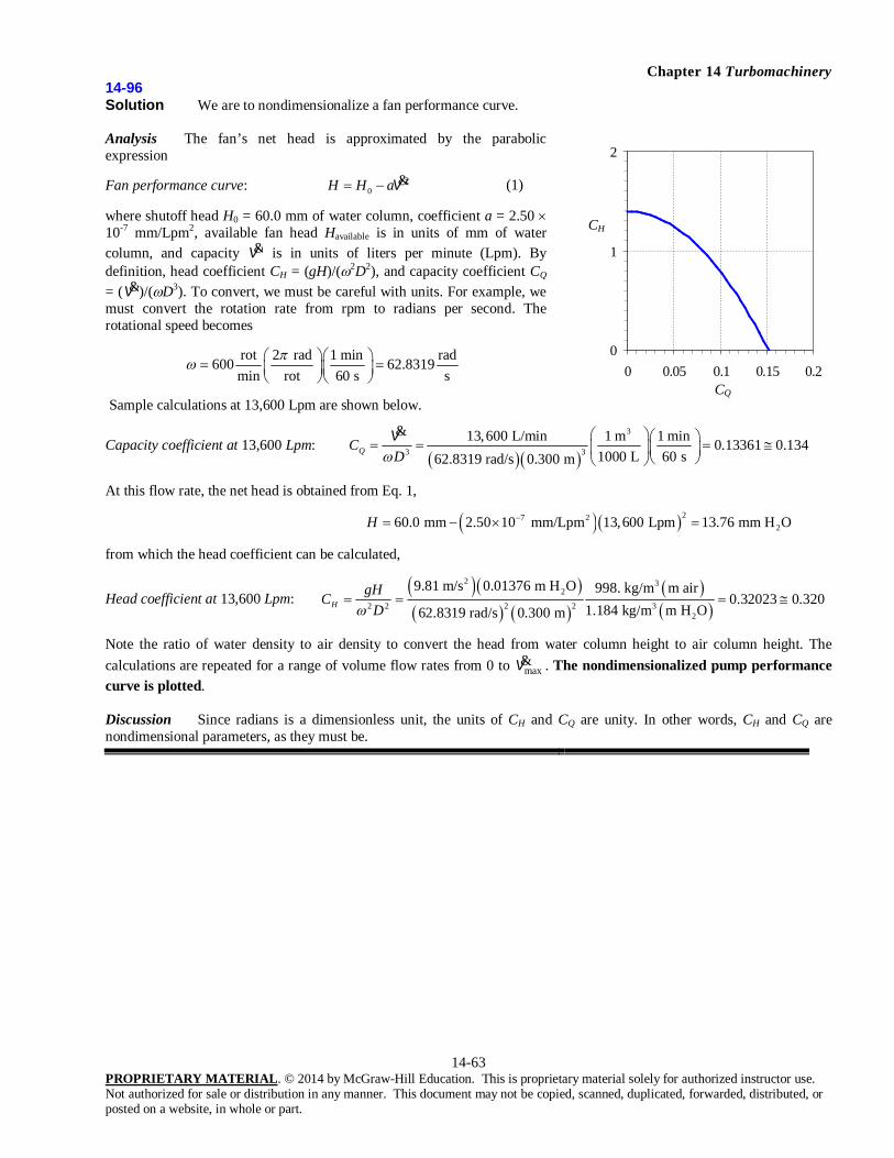
Chapter 14 Turbomachinery
14-63 PROPRIETARY MATERIAL. © 2014 by McGraw-Hill Education. This is proprietary material solely for authorized instructor use. Not authorized for sale or distribution in any manner. This document may not be copied, scanned, duplicated, forwarded, distributed, or posted on a website, in whole or part.
14-96 Solution We are to nondimensionalize a fan performance curve. Analysis The fan’s net head is approximated by the parabolic expression
Fan performance curve: 20H H a V& (1)
where shutoff head H0 = 60.0 mm of water column, coefficient a = 2.50 10-7 mm/Lpm2, available fan head Havailable is in units of mm of water column, and capacity V& is in units of liters per minute (Lpm). By definition, head coefficient CH = (gH)/(2D2), and capacity coefficient CQ = (V&)/(D3). To convert, we must be careful with units. For example, we must convert the rotation rate from rpm to radians per second. The rotational speed becomes
rot 2 rad 1 min rad600 62.8319min rot 60 s s
Sample calculations at 13,600 Lpm are shown below.
Capacity coefficient at 13,600 Lpm:
3
3 3
13,600 L/min 1 m 1 min 0.13361 0.1341000 L 60 s62.8319 rad/s 0.300 m
QCD
V&
At this flow rate, the net head is obtained from Eq. 1,
27 2260.0 mm 2.50 10 mm/Lpm 13,600 Lpm 13.76 mm H OH
from which the head coefficient can be calculated,
Head coefficient at 13,600 Lpm:
2 32
2 2 2 2 32
9.81 m/s 0.01376 m H O 998. kg/m m air0.32023 0.320
1.184 kg/m m H O62.8319 rad/s 0.300 mH
gHCD
Note the ratio of water density to air density to convert the head from water column height to air column height. The calculations are repeated for a range of volume flow rates from 0 to maxV& . The nondimensionalized pump performance curve is plotted. Discussion Since radians is a dimensionless unit, the units of CH and CQ are unity. In other words, CH and CQ are nondimensional parameters, as they must be.
0
1
2
0 0.05 0.1 0.15 0.2
CQ
CH

Chapter 14 Turbomachinery
14-64 PROPRIETARY MATERIAL. © 2014 by McGraw-Hill Education. This is proprietary material solely for authorized instructor use. Not authorized for sale or distribution in any manner. This document may not be copied, scanned, duplicated, forwarded, distributed, or posted on a website, in whole or part.
14-97 Solution We are to calculate the specific speed of a fan, and determine what kind of fan it is.
Analysis First, we use the values of CH and CQ calculated in the previous problem at the BEP (to four significant digits) to calculate the dimensionless form of NSp,
Dimensionless pump specific speed: 1/ 2 1/ 2
3 / 4 3 / 4
0.13361 0.85870.32023
QSp
H
CN
C
Thus, NSp = 0.859, and is dimensionless. From the conversion given in the text, NSp,US = 0.8587 2,734 = 2350. Alternatively, we can use the dimensional data to calculate NSp,US, the dimensional pump specific speed in US units,
1/ 2
1/ 2
,US 3 / 4 3 / 4
0.2642 gpm600 rpm 13,600 Lpm , rpm , gpm Lpm2350
, ft ft11.60 m0.3048 m
Sp
nN
H
V&&
Note that we use H = 11.60 m of air, since air is the fluid being pumped here. We calculate H as Hair = Hwater(water/air) = (0.01376 m of water)(998/1.184) = 11.60 m of air. From either the dimensionless or the dimensional pump specific speed, Fig. 14-73 shows that this is most likely a centrifugal fan (probably a squirrel cage fan).
Discussion We calculated the dimensional pump specific speed two ways as a check of our algebra, and (fortunately) the results agree.
14-98 Solution We are to calculate the specific speed of a water pump, and determine what kind of pump it is.
Analysis First, we use the values of CH and CQ calculated in Example 14-11 at the BEP to calculate the dimensionless form of NSp,
Dimensionless pump specific speed: 1/ 2 1/ 2
3 / 4 3/ 4
0.0112 0.4810.133
QSp
H
CN
C
Thus, NSp = 0.481. From the conversion given in the text, NSp,US = 1310. From Fig. 14-73, this is most likely a centrifugal pump.
Discussion From Fig. 14-73, the maximum efficiency one can expect from a centrifugal pump at this value of NSp is about 0.87 (87%). The actual pump efficiency is only 81.2% (from Example 14-11), so there is room for improvement in the design.
14-99 Solution We are to decide what king of pump should be designed for given performance criteria.
Analysis We calculate the pump specific speed at the given conditions,
302.0m) )(1.2m/s 81.9(
s 60min 1
L 1000m 1L/min) (14.0
rpmrad/s
602rpm) 1200(
)( 4/32
2/13
4/3
gH
NSp
1/2V
From Fig. 14-73, we see that Len should design a centrifugal pump. The maximum pump efficiency is about 0.81 (81%) (based on Fig. 14-73 again).
Discussion This value of NSp is, in fact, on the low end of the curve for centrifugal pumps, so a centrifugal pump is the best Len can do, in spite of the low efficiency.

Chapter 14 Turbomachinery
14-65 PROPRIETARY MATERIAL. © 2014 by McGraw-Hill Education. This is proprietary material solely for authorized instructor use. Not authorized for sale or distribution in any manner. This document may not be copied, scanned, duplicated, forwarded, distributed, or posted on a website, in whole or part.
14-100 Solution We are to calculate the performance of a modified pump.
Assumptions 1 The modified pump operates at the best efficiency point. 2 Pump diameter and fluid properties remain the same.
Analysis At homologous points, the affinity laws are used to estimate the operating conditions of the modified pump. We let the original pump be Pump A, and the modified pump be Pump B. We get
Volume flow rate: L/min 0.21)1(rpm 1200rpm 1800L/min) (14.0 3
3
A
B
A
BAB
DD
VV
and
Net head: m 70.2)1(rpm 1200rpm 1800m) (1.2
2
A
B2
A
BAB
DD
HH
The volume flow rate of the modified pump is 21.0 L/min; the net head is 2.70 m. The pump specific speed of the modified pump is
302.0m) )(2.70m/s 81.9(
s 60min 1
L 1000m 1L/min) (21.0
rpmrad/s
602rpm) 1800(
)( 4/32
2/13
4/3
gH
NSp
1/2V
Thus, NSp = 0.302, which is the same as that of the original pump. This is not surprising since the two pumps operate at homologous points.
Discussion When the rpm is increased by a factor of 1.5, all else being equal, the volume flow rate of the pump increases by a factor of (1.5)1, while the net head increases by a factor of (1.5)2. This agrees with the mnemonic given in the text: “Very Hard Problems are as easy as 1, 2, 3.” We would expect the power to increase by a factor of (1.5)3. The specific speed of the two pumps must match since they operate at homologous points.

Chapter 14 Turbomachinery
14-66 PROPRIETARY MATERIAL. © 2014 by McGraw-Hill Education. This is proprietary material solely for authorized instructor use. Not authorized for sale or distribution in any manner. This document may not be copied, scanned, duplicated, forwarded, distributed, or posted on a website, in whole or part.
14-101E Solution We are to decide what king of pump should be designed for given performance criteria.
Properties The density of water at 77oF is 62.24 lbm/ft3.
Analysis We calculate the pump specific speed at the given conditions,
1/ 23
1/ 2
3 / 4 3 / 42
2 rad/s 0.13368 ft 1 min300 rpm 2,500 gal/min 60 rpm 1 gal 60 s
0.31632.174 ft/s 45 ft
SpNgH
V&
From Fig. 14-73, we choose a centrifugal pump. The maximum pump efficiency is about 0.82 (82%) (based on Fig. 14-73 again). From the definition of pump efficiency, bhp = pumpV&gH. Thus, the required brake horsepower is
3 2 3 2
pump
62.24 lbm/ft 32.174 ft/s 45 ft 5.57 ft /s lbf s 1 hp19,025 ft lbf/s 34.6 hp0.82 32.174 lbm ft 550 ft lbf/s
gHbhp
V&
Thus, we expect that the pump will require about 35 hp to turn the shaft.
Discussion Most large water pumps are of the centrifugal variety. This problem may also be solved in terms of the dimensional pump specific speed in customary US units: NSp,US = 864.

Chapter 14 Turbomachinery
14-67 PROPRIETARY MATERIAL. © 2014 by McGraw-Hill Education. This is proprietary material solely for authorized instructor use. Not authorized for sale or distribution in any manner. This document may not be copied, scanned, duplicated, forwarded, distributed, or posted on a website, in whole or part.
14-102 Solution We are to nondimensionalize a pump performance curve. Analysis The pump’s net head is approximated by the parabolic expression
Pump performance curve: 20H H a V& (1)
where shutoff head H0 = 24.4 m of water column, coefficient a = 0.0678 m/Lpm2, available pump head Havailable is in units of meters of water column, and capacity V& is in units of liters per minute (Lpm). By definition, head coefficient CH = (gH)/(2D2), and capacity coefficient CQ = (V&)/(D3). To convert, we must be careful with units. For example, we must convert the rotation rate from rpm to radians per second. The rotational speed is
rot 2 rad 1 min rad4200 439.823min rot 60 s s
Sample calculations at 14.0 Lpm are shown below.
3
3 3
14.0 L/min 1 m 1 min 0.90966 0.09101000 L 60 s439.823 rad/s 0.0180 m
QCD
V&
At this flow rate (14.0 Lpm), the net head is obtained from Eq. 1,
2224.4 m 0.0678 m/Lpm 14.0 Lpm 11.111 m 11.1 mH
from which the head coefficient can be calculated,
2
2 2 2 2
9.81 m/s 11.111 m1.7391 1.74
439.823 rad/s 0.0180 mH
gHCD
These calculations are repeated for a range of volume flow rates from 0 to maxV& . The nondimensionalized pump performance curve is plotted. Discussion Since radians is a dimensionless unit, the units of CH and CQ are unity. In other words, CH and CQ are nondimensional parameters, as they must be.
0
1
2
3
4
0 0.05 0.1 0.15
CQ
CH

Chapter 14 Turbomachinery
14-68 PROPRIETARY MATERIAL. © 2014 by McGraw-Hill Education. This is proprietary material solely for authorized instructor use. Not authorized for sale or distribution in any manner. This document may not be copied, scanned, duplicated, forwarded, distributed, or posted on a website, in whole or part.
14-103 Solution We are to calculate the specific speed of a water pump, and determine what kind of pump it is. Analysis First, we use the values of CH and CQ calculated in the previous problem at the BEP to calculate the dimensionless form of NSp,
Dimensionless pump specific speed: 1/ 2 1/ 2
3/ 4 3 / 4
0.090966 0.19921.7391
QSp
H
CN
C
Thus, NSp = 0.199, and is dimensionless. From the conversion given in the text, NSp,US = 0.1992 2,734 = 545. Alternatively, we can use the original dimensional data to calculate NSp,US,
Dimensional pump specific speed in customary US units:
1/ 2
1/ 2
,US 3 / 4 3 / 4
0.2642 gpm4200 rpm 14.0 Lpm , rpm , gpm Lpm545
, ft ft11.111 m0.3048 m
Sp
nN
H
V&&
From either the dimensionless or the dimensional pump specific speed, Fig. 14-73 shows that this is definitely a centrifugal pump. Discussion We calculated the dimensional pump specific speed two ways as a check of our algebra, and (fortunately) the results agree.
14-104 Solution We are to prove the relationship between turbine specific speed and pump specific speed. Assumptions 1 The parameters such as net head, volume flow rate, diameter, etc. are defined in similar fashion for the pump and the turbine. Analysis First we write the definitions of pump specific speed and turbine specific speed,
Pump specific speed:
1/ 2
3 / 4SpNgH
V&
(1)
and
Turbine specific speed:
1/ 2
1/ 2 5 / 4St
bhpN
gH
(2)
After some rearrangement of Eq. 2,
1/ 21/ 2
3 / 4StbhpNgHgH
VV
&& (3)
We recognize the first grouping of terms in Eq. 3 as NSp and the second grouping of terms as the square root of turbine efficiency turbine. Thus,
Final relationship: turbineSt SpN N (4)
Discussion Since turbine efficiency is typically large (90 to 95% for large hydroturbines), pump specific speed and turbine specific speed are nearly equivalent. Note that Eq. 4 does not apply to a pump running backwards as a turbine or vice-versa. Such devices, called pump-turbines, are addressed in the next problem.

Chapter 14 Turbomachinery
14-69 PROPRIETARY MATERIAL. © 2014 by McGraw-Hill Education. This is proprietary material solely for authorized instructor use. Not authorized for sale or distribution in any manner. This document may not be copied, scanned, duplicated, forwarded, distributed, or posted on a website, in whole or part.
14-105 Solution We are to prove the relationship between turbine specific speed and pump specific speed for the case of a pump-turbine operating at the same volume flow rate and rotational speed when acting as a pump and as a turbine. Assumptions 1 The parameters such as net head, volume flow rate, diameter, etc. are defined in similar fashion for the pump and the turbine. Analysis First we write the definitions of pump specific speed and turbine specific speed,
Pump specific speed:
1/ 2
3 / 4
pump
SpNgH
V& (1)
and
Turbine specific speed:
1/ 2turbine
1/ 2 5 / 4turbine
St
bhpN
gH
(2)
Note that we have added subscripts “pump” and “turbine” on net head and brake horsepower since Hpump Hturbine and bhppump bhpturbine. After some rearrangement of Eq. 2,
1/ 2
1/ 2 1/ 21/ 2turbine
turbine3 / 4 3 / 4turbineturbine turbine
Stbhp
NgHgH gH
V VV
& && (3)
We also write the definitions of pump efficiency and turbine efficiency,
pump turbinepump turbine
pump turbine
g H bhpbhp g H
VV
&& (4)
We solve both parts of Eq. 4 for V& and equate the two, since V& is the same whether the pump-turbine is operating as a pump or as a turbine. Eliminating V&,
pump turbineturbine
pump pump turbine
H bhpH
bhp (5)
where and g have also dropped out since they are the same for both cases. We plug Eq. 5 into Eq. 3 and rearrange,
3 / 41/ 2
1/ 2 pump pump turbineturbine3 / 4
turbinepump
St
bhpN
bhpgH
V& (6)
We recognize the first grouping of terms in Eq. 6 as NSp and rearrange,
Final relationship: 3 / 4
3 / 45 / 4 pumpturbine pump
turbineSt Sp
bhpN N
bhp
(7)
An alternate expression is obtained in terms of net heads by substitution of Eq. 5,
Alternate final relationship: 3 / 4
pumpturbine
turbineSt Sp
HN N
H
(8)
Discussion It is difficult to achieve high efficiency in a pump-turbine during both the pump duty cycle and the turbine duty cycle. To achieve the highest possible efficiency, it is critical that both NSp and NSt are appropriate for the chosen design, e.g. radial flow centrifugal pump and radial-flow Francis turbine.
Chapter 14 Turbomachinery
14-70 PROPRIETARY MATERIAL. © 2014 by McGraw-Hill Education. This is proprietary material solely for authorized instructor use. Not authorized for sale or distribution in any manner. This document may not be copied, scanned, duplicated, forwarded, distributed, or posted on a website, in whole or part.
14-106 Solution We are to apply conversion factors to prove a conversion factor. Properties We set g = 32.174 ft/s2 and assume water at density = 1.94 slug/ft3. Analysis We convert NSt,US to NSt by dividing by g5/4 and 1/2, and then using conversion ratios to cancel all units,
,US
1/ 2 1/ 21/ 2
5 / 4 1/ 2 5 / 4 23 2
, rot/min , hp 1 1 min slug ft 550 ft lbf 2 rad60 s s hp ss lbf, ft 1.94 slug/ft 32.174 ft/s
St
St
N
bhpN
H
1 4 4 4 4 2 4 4 4 43
US= 0.02301St St,N N
Finally, the inverse of the above equation yields the desired conversion factor. Discussion As discussed in the text, some turbomachinery authors do not convert rotations to radians, introducing a confusing factor of 2 into the conversion.
14-107 Solution We are to calculate the specific speed of a turbine, and compare it to the normal range. Analysis We first calculate the nondimensional form of NSt,
1/ 2 1/ 21/ 2 8 2
5 / 4 5 / 4 31/ 21/ 2 3 2
18.85 rad/s 2.46 10 W kg mW s998.0 kg/m 9.81 m/s 73.8 m
St
bhpN
gH
2.49
From Fig. 14-108, this is much higher than the typical Francis turbine – the designers should consider a Kaplan turbine instead. From the conversion given in the text, NSt,US = 2.49 43.46 = 108. Alternatively, we can use the original dimensional data to calculate NSt,US,
1/ 21/ 2 5
,US 5 / 4 5 / 4
180 rpm 3.29 10 hp, rpm , hp
, ft ft73.8 m0.3048 m
St
n bhpN
H
108&
Note that the actual values of brake horsepower and net head will differ from the values calculated here, because we have neglected irreversible losses; thus, the values of NSt and NSt,US may change slightly. Discussion We calculated the dimensional pump specific speed two ways as a check of our algebra, and the results agree.

Chapter 14 Turbomachinery
14-71 PROPRIETARY MATERIAL. © 2014 by McGraw-Hill Education. This is proprietary material solely for authorized instructor use. Not authorized for sale or distribution in any manner. This document may not be copied, scanned, duplicated, forwarded, distributed, or posted on a website, in whole or part.
14-108 Solution We are to calculate turbine specific speed for a given hydroturbine and compare to the guidelines of Fig. 14-116. Assumptions 1 The fluid is water at 20oC. Properties The density of water at 20oC is = 998.0 kg/m3. Analysis First we convert the turbine rotation rate from rpm to radians/s,
Rotational speed: rot 2 rad 1 min100 10.47 rad/smin rot 60 s
With all other parameters already given in SI units, we calculate turbine specific speed,
1/ 2 1/ 21/ 2 6 2
1/ 2 5 / 4 5 / 4 31/ 23 2
10.47 rad/s 194 10 W m kgs W998 kg/m 9.81 m/s 54.9 m
St
bhpN
gH
1.78
Comparing to the turbine specific speed guidelines of Fig. 14-108, we see that this turbine should be of the Francis type, which it is. Discussion The turbine specific speed of this turbine is close to the crossover point between a Francis turbine and a Kaplan turbine.
14-109 Solution We are to calculate turbine specific speed for a given hydroturbine and compare to the guidelines of Fig. 14-116. Assumptions 1 The fluid is water at 20oC. Properties The density of water at 20oC is = 998.0 kg/m3. Analysis First we convert the turbine rotation rate from rpm to radians/s,
Rotational speed: rot 2 rad 1 min100 10.47 rad/smin rot 60 s
With all other parameters already given in SI units, we calculate turbine specific speed,
1/ 2 1/ 21/ 2 6 2
1/ 2 5 / 4 5 / 4 31/ 23 2
10.47 rad/s 5.37 10 W m kgs W998 kg/m 9.81 m/s 9.75 m
St
bhpN
gH
2.57
Comparing to the turbine specific speed guidelines of Fig. 14-108, we see that this turbine should be of the Kaplan type, which it is. Discussion In fact, the turbine specific speed of this turbine is close to that which yields the maximum possible efficiency for a Kaplan turbine.

Chapter 14 Turbomachinery
14-72 PROPRIETARY MATERIAL. © 2014 by McGraw-Hill Education. This is proprietary material solely for authorized instructor use. Not authorized for sale or distribution in any manner. This document may not be copied, scanned, duplicated, forwarded, distributed, or posted on a website, in whole or part.
14-110 Solution We are to calculate the specific speed of a turbine, and compare it to the normal range. Analysis We first calculate the nondimensional form of NSt,
1/ 2 1/ 21/ 2 8 2
5 / 4 5 / 4 31/ 21/ 2 3 2
12.57 rad/s 4.61 10 W kg mW s998.0 kg/m 9.81 m/s 78.6 m
St
bhpN
gH
2.10
From Fig. 14-108, this is on the high end for Francis turbines – the designers may wish to consider a Kaplan turbine instead. From the conversion given in the text, NSt,US = 2.10 43.46 = 91.4. Alternatively, we can use the original dimensional data to calculate NSt,US,
1/ 21/ 2 5
,US 5 / 4 5 / 4
120 rpm 6.18 10 hp, rpm , hp
, ft ft78.6 m0.3048 m
St
n bhpN
H
91.3&
Note that the actual values of brake horsepower and net head will differ from the values calculated here, because we have neglected irreversible losses; thus, the values of NSt and NSt,US may change slightly. Discussion We calculated the dimensional pump specific speed two ways as a check of our algebra, and (fortunately) the results agree (within round-off error).
14-111 Solution We are to calculate the specific speed of a turbine, and compare it to the normal range. Analysis We first calculate the nondimensional form of NSt,
1/ 2 1/ 21/ 2 7 2
5 / 4 5 / 4 31/ 21/ 2 3 2
12.5664 rad/s 4.6302 10 W kg mW s998.0 kg/m 9.81 m/s 59.117 m
St
bhpN
gH
0.951
From Fig. 14-108, this is in the range of the typical Francis turbine. From the conversion given in the text, NSt,US = 0.951 43.46 = 41.3. Alternatively, we can use the original dimensional data to calculate NSt,US,
1/ 21/ 2 4
,US 5 / 4 5 / 4
120 rpm 6.209 10 hp, rpm , hp
, ft 193.95 ftSt
n bhpN
H
41.3
&
Note that the actual values of brake horsepower and net head will differ from the values calculated here, because we have neglected irreversible losses; thus, the values of NSt and NSt,US may change slightly. Discussion We calculated the dimensional pump specific speed two ways as a check of our algebra, and the results agree.

Chapter 14 Turbomachinery
14-73 PROPRIETARY MATERIAL. © 2014 by McGraw-Hill Education. This is proprietary material solely for authorized instructor use. Not authorized for sale or distribution in any manner. This document may not be copied, scanned, duplicated, forwarded, distributed, or posted on a website, in whole or part.
14-112E Solution We are to calculate the specific speed of a turbine, and compare it to the normal range. Analysis We first calculate the specific speed in customary US units,
1/ 2 1/ 2
,US 5 / 4 5 / 4
, rpm , hp 120 rpm 202,700 hp
, ft 170.8 ftSt
n bhpN
H 87.5
&
From Fig. 14-108, this is on the high end of typical Francis turbines, on the border between Francis and Kaplan turbines. In nondimensional terms, NSt,US = 87.5 / 43.46 = 2.01. Note that the actual values of brake horsepower and net head will differ from the values calculated here, because we have neglected irreversible losses; thus, the values of NSt and NSt,US may change slightly. Discussion The actual values of brake horsepower and net head will differ from the values calculated here, because we have neglected irreversible losses; thus, the values of NSt and NSt,US may change slightly.
14-113 Solution We are to calculate turbine specific speed for a given hydroturbine and compare to the guidelines of Fig. 14-116. Assumptions 1 The fluid is water at 20oC. Properties The density of water at 20oC is = 998.0 kg/m3. Analysis First we convert the turbine rotation rate from rpm to radians/s,
Rotational speed: rot 2 rad 1 min180 18.85 rad/smin rot 60 s
With all other parameters already given in SI units, we calculate turbine specific speed,
1/ 2 1/ 21/ 2 6 2
1/ 2 5 / 4 5 / 4 31/ 23 2
18.85 rad/s 119 10 W m kgs W998 kg/m 9.81 m/s 105 m
St
bhpN
gH
1.12
Comparing to the turbine specific speed guidelines of Fig. 14-108, we see that this turbine should be of the Francis type, which it is. Discussion In fact, the turbine specific speed of this turbine is close to that which yields the maximum possible efficiency for a Francis turbine.

Chapter 14 Turbomachinery
14-74 PROPRIETARY MATERIAL. © 2014 by McGraw-Hill Education. This is proprietary material solely for authorized instructor use. Not authorized for sale or distribution in any manner. This document may not be copied, scanned, duplicated, forwarded, distributed, or posted on a website, in whole or part.
14-114 Solution We are to determine a turbine’s efficiency and what kind of turbine is being tested. Properties The density of water at T = 20oC is 998.0 kg/m3. Analysis The turbine’s efficiency is calculated first,
69.2%
6922.0
sWmkg
hs 3600
/h)m m)(25.5 )(15.0m/s 81.9)(kg/m 0.998( W720
3
2
323turbine VgHbhp
After converting 1500 rpm to 157.1 rad/s, we calculate the nondimensional form of turbine specific speed,
260.0sWmkg
m) )(15.0m/s 81.9()kg/m 0.998(
W)rad/s)(720 (157.1)(
)(3
2
4/522/13
1/2
4/52/1
2/1
gHbhpNSt
which we convert to customary US units, NSt,US = 0.260 43.46 = 11.3. This is most likely an impulse turbine (e.g., a Pelton wheel turbine). Discussion We could instead have used the dimensional units to directly calculate the turbine specific speed in customary US units. The result would be the same.
14-115 Solution We are to scale up the model turbine tests to the prototype turbine. Assumptions 1 The prototype and model are geometrically similar. 2 The tests are conducted under conditions of dynamic similarity. 3 The water is at the same temperature for both the model and the prototype (20oC). Properties The density of water at T = 20oC is 998.0 kg/m3. Analysis We use the turbine scaling laws, starting with the head coefficient, and letting the model be turbine A and the prototype be turbine B,
A B A B,A ,B B A B2 2 2 2
B AA A B B
1 50 m 1500 rpm5 15.0 mH H
gH gH D HC CD HD D
548 rpm
We then use the capacity coefficient to calculate the volume flow rate of the prototype,
/hm 1160 3
/hm 5.1164
15
rpm 1500rpm 548/h)m (25.5 3
33
3
A
B
A
BAB,3
B
B3
A
A, D
DC
DDC BQ
BAAQ
VV
VV
Finally, we use the power coefficient to calculate the brake horsepower of the prototype,
W110,000
W711,109
15
rpm 1500rpm 548 W)(720
535
A
B3
A
BAB,53
B53
A, D
DbhpbhpC
Dbhp
Dbhp
C BPBBAA
AP
Discussion All results are given to 3 significant digits, but we kept several extra digits in the intermediate calculations to reduce round-off errors.

Chapter 14 Turbomachinery
14-75 PROPRIETARY MATERIAL. © 2014 by McGraw-Hill Education. This is proprietary material solely for authorized instructor use. Not authorized for sale or distribution in any manner. This document may not be copied, scanned, duplicated, forwarded, distributed, or posted on a website, in whole or part.
14-116 Solution We are to compare the model and prototype efficiency and turbine specific speed to prove that they operate at homologous points. Properties The density of water at T = 20oC is 998.0 kg/m3. Analysis The model turbine’s efficiency was calculated in Problem 14-119 as 69.2%. We calculate the prototype turbine’s efficiency as
69.3%
6929.0
sWmkg
hs 3600
/h)m m)(1164.5 )(50m/s 81.9)(kg/m 0.998( W109,711
3
2
323turbine VgHbhp
The efficiency of the prototype is practically the same as that of the model. Similarly, the turbine specific speed of the model turbine was calculated previously as 0.260. After converting 548 rpm to 57.36 rad/s, we calculate the nondimensional form of turbine specific speed for the prototype turbine,
261.0sWmkg
m) )(50m/s 81.9()kg/m 0.998(
W),711rad/s)(109 (57.36)(
)(3
2
4/522/13
1/2
4/52/1
2/1
gHbhpNSt
which is also practically the same as the previous calculation. Comparing to the results of Problem 14-119, we see that both turbine and Nst match between the model and the prototype. Thus, the model and the prototype operate at homologous points. Discussion Other nondimensional turbine parameters, like head coefficient, capacity coefficient, and power coefficient also match between model and prototype. We could instead have used dimensional units to calculate the turbine specific speed in customary US units.

Chapter 14 Turbomachinery
14-76 PROPRIETARY MATERIAL. © 2014 by McGraw-Hill Education. This is proprietary material solely for authorized instructor use. Not authorized for sale or distribution in any manner. This document may not be copied, scanned, duplicated, forwarded, distributed, or posted on a website, in whole or part.
14-117 Solution We are to estimate the actual efficiency of the prototype, and explain why it is higher than the model efficiency. Analysis We apply the Moody efficiency correction equation,
77.7%
7768.0
51)692.01(1)1(1
5/15/1
protottype
modelmodel turbine,prototype turbine, D
D
This represents an increase of 77.7 – 69.2 = 8.5%. However, as mentioned in the text, we expect only about 2/3 of this increase, or 2(8.5%)/3 = 5.7%. Thus, our best estimate of the actual efficiency of the prototype is 68.6% 7.59.62prototype turbine, There are several reasons for this increase in efficiency: The prototype turbine often operates at high Reynolds numbers that are not achievable in the laboratory. We know from the Moody chart that friction factor decreases with Re, as does boundary layer thickness. Hence, the influence of viscous boundary layers is less significant as turbine size increases, since the boundary layers occupy a less significant percentage of the flow path through the runner. In addition, the relative roughness (/D) on the surfaces of the prototype runner blades may be significantly smaller than that on the model turbine unless the model surfaces are micropolished. Finally, large full scale turbines have smaller tip clearances relative to blade diameter; therefore tip losses and leakage are less significant. Discussion The increase in efficiency between the model and prototype is significant, and helps us to understand why very large hydroturbines can be extremely efficient devices.

Chapter 14 Turbomachinery
14-77 PROPRIETARY MATERIAL. © 2014 by McGraw-Hill Education. This is proprietary material solely for authorized instructor use. Not authorized for sale or distribution in any manner. This document may not be copied, scanned, duplicated, forwarded, distributed, or posted on a website, in whole or part.
Review Problems
14-118C Solution We are to discuss the definition and usefulness of a pump-turbine. Analysis A pump-turbine is a turbomachine that can run both as a pump and as a turbine (by running in the opposite direction). A pump-turbine is used by some power plants for energy storage; specifically, water is pumped by the pump-turbine during periods of low demand for power, and electricity is generated by the pump-turbine during periods of high demand for power. Discussion We note that energy is “lost” both ways – when the pump-turbine is acting as a pump, and when it is acting as a turbine. Nevertheless, the energy storage scheme may still be cost-effective and profitable, in spite of the energy losses, because it may enable a power company to delay construction of costly new power-production facilities.
14-119C Solution We are to discuss a water meter from the point of view of a piping system. Analysis Although a water meter is a type of turbine, when analyzing pipe flow systems, we would think of the water meter as a type of minor loss in the system, just as a valve, elbow, etc. would be a minor loss, since there is a pressure drop associated with flow through the water meter. Discussion In fact, manufacturers of water meters provide minor loss coefficients for their products.
14-120C Solution (a) True: As the gears turn, they direct a closed volume of fluid from the inlet to the outlet of the gear pump. (b) True or False: Rotary pumps can be either positive displacement or dynamic (an unfortunate use of terminology). As a
positive-displacement pump, the rotors direct a closed volume of fluid from the inlet to the outlet of the rotary pump. As a dynamic pump, “rotary pump” is sometimes used in place of the more correct term, “rotodynamic pump”.
(c) True: At a given rotational speed, the volume flow rate of a positive-displacement pump is fairly constant regardless of load because of the fixed closed volume.
(d) False: Actually, the net head increases with fluid viscosity, because high viscosity fluids cannot penetrate the gaps as easily.
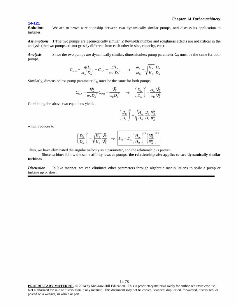
Chapter 14 Turbomachinery
14-78 PROPRIETARY MATERIAL. © 2014 by McGraw-Hill Education. This is proprietary material solely for authorized instructor use. Not authorized for sale or distribution in any manner. This document may not be copied, scanned, duplicated, forwarded, distributed, or posted on a website, in whole or part.
14-121 Solution We are to prove a relationship between two dynamically similar pumps, and discuss its application to turbines. Assumptions 1 The two pumps are geometrically similar. 2 Reynolds number and roughness effects are not critical in the analysis (the two pumps are not grossly different from each other in size, capacity, etc.). Analysis Since the two pumps are dynamically similar, dimensionless pump parameter CH must be the same for both pumps,
A B A A B,A H,B2 2 2 2
B B AA A B B
HgH gH H DC C
H DD D
Similarly, dimensionless pump parameter CQ must be the same for both pumps,
3
A B B A B,A ,B3 3
A BA A B B A
Q QD
C CDD D
V V VV
& & &&
Combining the above two equations yields
3
B A B B
A B A A
D H DD H D
VV
&&
which reduces to
2
B A B
A B A
D HD H
VV
&&
1/ 21/ 4
A BB A
B A
HD D
H
VV
&&
Thus, we have eliminated the angular velocity as a parameter, and the relationship is proven. Since turbines follow the same affinity laws as pumps, the relationship also applies to two dynamically similar turbines. Discussion In like manner, we can eliminate other parameters through algebraic manipulations to scale a pump or turbine up or down.

Chapter 14 Turbomachinery
14-79 PROPRIETARY MATERIAL. © 2014 by McGraw-Hill Education. This is proprietary material solely for authorized instructor use. Not authorized for sale or distribution in any manner. This document may not be copied, scanned, duplicated, forwarded, distributed, or posted on a website, in whole or part.
14-122 Solution We are to prove a relationship between two dynamically similar turbines, and discuss its application to pumps. Assumptions 1 The two turbines are geometrically similar. 2 Reynolds number and roughness effects are not critical in the analysis (the two turbines are not grossly different from each other in size, capacity, etc.). Analysis Since the two turbines are dynamically similar, dimensionless turbine parameter CH must be the same for both turbines,
A B A A B,A H,B2 2 2 2
B B AA A B B
HgH gH H DC C
H DD D
Similarly, dimensionless turbine parameter CP must be the same for both turbines,
5 3
A B B A A B,A ,B3 5 3 5
A B B AA A A B B B
P Qbhp bhp D bhp
C CD bhpD D
Combining the above two equations yields
5 3/ 2 3
B A B A B
A B A B A
D H D bhpD H D bhp
which reduces to
2 3 / 2
B A A B
A B B A
D H bhpD H bhp
3 / 4 1/ 2 1/ 2
A A BB A
B B A
H bhpD D
H bhp
Thus, we have eliminated the angular velocity as a parameter, and the relationship is proven. Since pumps follow the same affinity laws as turbines, the relationship also applies to two dynamically similar pumps. Discussion In like manner, we can eliminate other parameters through algebraic manipulations to scale a pump or turbine up or down.

Chapter 14 Turbomachinery
14-80 PROPRIETARY MATERIAL. © 2014 by McGraw-Hill Education. This is proprietary material solely for authorized instructor use. Not authorized for sale or distribution in any manner. This document may not be copied, scanned, duplicated, forwarded, distributed, or posted on a website, in whole or part.
14-123 Solution We are to design a new hydroturbine by scaling up an existing hydroturbine. Specifically we are to calculate the new turbine diameter, volume flow rate, and brake horsepower.
Assumptions 1 The new turbine is geometrically similar to the existing turbine. 2 Reynolds number effects and roughness effects are negligible. 3 The new penstock is also geometrically similar to the existing penstock so that the flow entering the new turbine (velocity profile, turbulence intensity, etc.) is similar to that of the existing turbine.
Properties The density of water at 20oC is = 998.0 kg/m3.
Analysis Since the new turbine (B) is dynamically similar to the existing turbine (A), we are concerned with only one particular homologous operating point of both turbines, namely the best efficiency point. We solve Eq. 14-38b for DB,
m 2.20
2.2016
rpm 105rpm 150
m 90.0m 95m) (1.50
B
A
A
BAB n
nHH
DD
We then solve Eq. 14-38a for BV&,
/hm 359 3
/hm 5.358
m 1.50m 2.2016
rpm 150rpm 105/s)m (162 3
33
3
A
B
A
BAB D
Dnn VV
Finally, we solve Eq. 14-38c for bhpB,
MW 308
MW 4.308
m 1.50m 2.2016
rpm 150rpm 105MW)(1) (132
535
A
B3
A
B
A
BAB D
Dnn
bhpbhp
Discussion To avoid round-off errors, we save several more significant digits for DB than are given in the final answer.
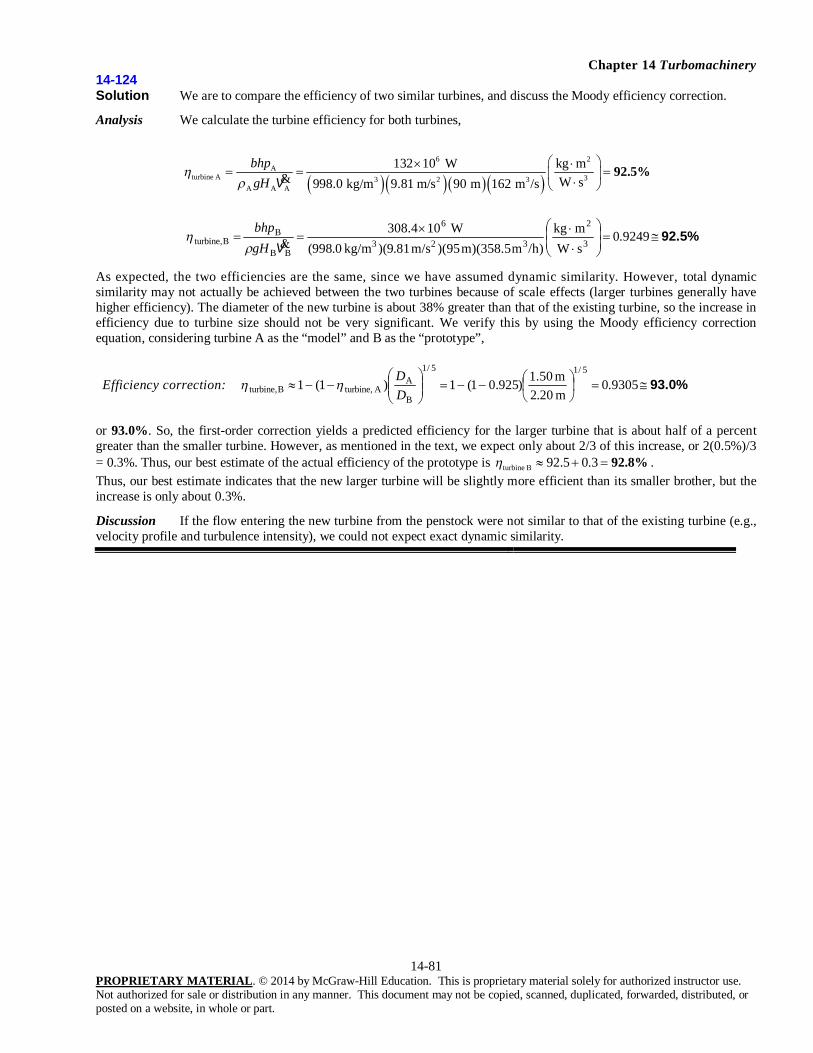
Chapter 14 Turbomachinery
14-81 PROPRIETARY MATERIAL. © 2014 by McGraw-Hill Education. This is proprietary material solely for authorized instructor use. Not authorized for sale or distribution in any manner. This document may not be copied, scanned, duplicated, forwarded, distributed, or posted on a website, in whole or part.
14-124 Solution We are to compare the efficiency of two similar turbines, and discuss the Moody efficiency correction.
Analysis We calculate the turbine efficiency for both turbines,
6 2A
turbine A 33 2 3A A A
132 10 W kg mW s998.0 kg/m 9.81 m/s 90 m 162 m /s
bhpgH
92.5%V&
92.5%
9249.0
sWmkg
/h)m m)(358.5 )(95m/s 81.9)(kg/m 0.998( W10308.4
3
2
323
6
BB
BBturbine, VgH
bhp
As expected, the two efficiencies are the same, since we have assumed dynamic similarity. However, total dynamic similarity may not actually be achieved between the two turbines because of scale effects (larger turbines generally have higher efficiency). The diameter of the new turbine is about 38% greater than that of the existing turbine, so the increase in efficiency due to turbine size should not be very significant. We verify this by using the Moody efficiency correction equation, considering turbine A as the “model” and B as the “prototype”,
Efficiency correction: 93.0%
9305.0
m 20.2m 1.50)925.01(1)1(1
5/15/1
B
AA turbine,Bturbine, D
D
or 93.0%. So, the first-order correction yields a predicted efficiency for the larger turbine that is about half of a percent greater than the smaller turbine. However, as mentioned in the text, we expect only about 2/3 of this increase, or 2(0.5%)/3 = 0.3%. Thus, our best estimate of the actual efficiency of the prototype is turbine B 92.5 0.3 92.8% . Thus, our best estimate indicates that the new larger turbine will be slightly more efficient than its smaller brother, but the increase is only about 0.3%.
Discussion If the flow entering the new turbine from the penstock were not similar to that of the existing turbine (e.g., velocity profile and turbulence intensity), we could not expect exact dynamic similarity.

Chapter 14 Turbomachinery
14-82 PROPRIETARY MATERIAL. © 2014 by McGraw-Hill Education. This is proprietary material solely for authorized instructor use. Not authorized for sale or distribution in any manner. This document may not be copied, scanned, duplicated, forwarded, distributed, or posted on a website, in whole or part.
14-125 Solution The turbine specific speed of two dynamically similar turbines is to be compared, and the most likely type of turbine is to be determined.
Properties The density of water at T = 20oC is = 998.0 kg/m3.
Analysis We calculate the dimensionless turbine specific speed for turbines A and B,
1/ 2 1/ 21/ 2 6 2A A
,A 1/ 2 5 / 4 5 / 4 31/ 23 2A A
15.71 rad/s 132 10 W kg mW s998.0 kg/m 9.81 m/s 90.0 m
St
bhpN
gH
1.19
1.19
3
2
4/522/13
1/26
4/5B
2/1B
2/1BB
,sWmkg
m) )(95m/s 81.9()kg/m 0.998(
W)10.4rad/s)(308 (11.00)()(
)(gH
bhpN BSt
We see that the turbine specific speed of the two turbines is the same. In customary US units,
,US,A ,US,B 43.46 43.46 1.19St St StN N N 51.6
From Fig. 14-108, both of these turbines are most likely Francis turbines. Discussion Since turbine A and turbine B operate at homologous points, it is no surprise that their turbine specific speeds are the same. In fact, if they weren’t the same, it would be a sure sign of an algebraic or calculation error.

Chapter 14 Turbomachinery
14-83 PROPRIETARY MATERIAL. © 2014 by McGraw-Hill Education. This is proprietary material solely for authorized instructor use. Not authorized for sale or distribution in any manner. This document may not be copied, scanned, duplicated, forwarded, distributed, or posted on a website, in whole or part.
Fundamentals of Engineering (FE) Exam Problems
14-126
Which turbomachine is designed to deliver a very high pressure rise, typically at low to moderate flow rates?
(a) Compressor (b) Blower (c) Turbine (d) Pump (e) Fan
Answer (a) Compressor
14-127
In the turbomachinery industry, capacity refers to
(a) Power (b) Mass flow rate (c) Volume flow rate (d) Net head
(e) Energy grade line
Answer (c) Volume flow rate
14-128
A pump increases the pressure of water from 100 kPa to 3 MPa at a rate of 0.5 m3/min. The inlet and outlet diameters are identical and there is no change in elevation across the pump. If the efficiency of the pump is 77 percent, the power supplied to the pump is
(a) 18.5 kW (b) 21.8 kW (c) 24.2 kW (d) 27.6 kW (e) 31.4 kW
Answer (e) 31.4 kW
Solution Solved by EES Software. Solutions can be verified by copying-and-pasting the following lines on a blank EES screen. (Similar problems and their solutions can be obtained easily by modifying numerical values). P_in=100 [kPa] P_out=3000 [kPa] V_dot=0.5 [m^3/min]*Convert(m^3/min, m^3/s) eta_pump=0.77 W_dot_useful=V_dot*(P_out-P_in) W_dot_shaft=W_dot_useful/eta_pump

Chapter 14 Turbomachinery
14-84 PROPRIETARY MATERIAL. © 2014 by McGraw-Hill Education. This is proprietary material solely for authorized instructor use. Not authorized for sale or distribution in any manner. This document may not be copied, scanned, duplicated, forwarded, distributed, or posted on a website, in whole or part.
14-129
A pump increases the pressure of water from 100 kPa to 900 kPa to an elevation of 35 m. The inlet and outlet diameters are identical. The net head of the pump is
(a) 143 m (b) 117 m (c) 91 m (d) 70 m (e) 35 m
Answer (b) 117 m
Solution Solved by EES Software. Solutions can be verified by copying-and-pasting the following lines on a blank EES screen. (Similar problems and their solutions can be obtained easily by modifying numerical values). P_in=100000 [Pa] P_out=900000 [Pa] z_in=0 [m] z_out=35 [m] g=9.81 [m/s^2] rho=1000 [kg/m^3] H=P_out/(rho*g)+z_out-P_in/(rho*g)-z_in
14-130
The brake horsepower and water horsepower of a pump are determined to be 15 kW and 12 kW, respectively. If the flow rate of water to the pump under these conditions is 0.05 m3/s, the total head loss of the pump is
(a) 11.5 m (b) 9.3 m (c) 7.7 m (d) 6.1 m (e) 4.9 m
Answer (d) 6.1 m
Solution Solved by EES Software. Solutions can be verified by copying-and-pasting the following lines on a blank EES screen. (Similar problems and their solutions can be obtained easily by modifying numerical values). W_dot_in=15000 [W] W_dot_useful=12000 [W] V_dot=0.05 [m^3/s] g=9.81 [m/s^2] rho=1000 [kg/m^3] W_dot_loss=W_dot_in-W_dot_useful H=W_dot_loss/(rho*g*V_dot)
14-131
In the pump performance curve, the point at which the net head is zero is called
(a) Best efficiency point (b) Free delivery (c) Shutoff head (d) Operating point
(e) Duty point
Answer (b) Free delivery

Chapter 14 Turbomachinery
14-85 PROPRIETARY MATERIAL. © 2014 by McGraw-Hill Education. This is proprietary material solely for authorized instructor use. Not authorized for sale or distribution in any manner. This document may not be copied, scanned, duplicated, forwarded, distributed, or posted on a website, in whole or part.
14-132
A power plant requires 940 L/min of water. The required net head is 5 m at this flow rate. An examination of pump performance curves indicates that two centrifugal pumps with different impeller diameters can deliver this flow rate. The pump with an impeller diameter of 203 mm has a pump efficiency of 73 percent and delivers 10 m of net head. The pump with an impeller diameter of 111 mm has a lower pump efficiency of 67 percent and but delivers 5 m of net head. What is the ratio of the required brake horse power (bhp) of the pump with 203-mm-diameter impeller to that of the pump with 111-mm-diameter impeller?
(a) 0.45 (b) 0.68 (c) 0.86 (d) 1.84 (e) 2.11
Answer (d) 1.84
Solution Solved by EES Software. Solutions can be verified by copying-and-pasting the following lines on a blank EES screen. (Similar problems and their solutions can be obtained easily by modifying numerical values). V_dot=940 [L/min]*Convert(L/min, m^3/s) H_required=5 [m] H_1=10 [m] H_2=5 [m] eta_pump_1=0.73 eta_pump_2=0.67 g=9.81 [m/s^2] rho=1000 [kg/m^3] bhp_1=rho*g*V_dot*H_1/eta_pump_1 bhp_2=rho*g*V_dot*H_2/eta_pump_2 bhp_Ratio=bhp_1/bhp_2 "or" bhpRatio=(H_1/eta_pump_1)/(H_2/eta_pump_2)
14-133
Water enters the pump of a steam power plant at 20 kPa and 50C at a rate of 0.15 m3/s. The diameter of the pipe at the pump inlet is 0.25 m. What is the net positive suction head (NPSH) at the pump inlet?
(a) 2.14 m (b) 1.89 m (c) 1.66 m (d) 1.42 m (e) 1.26 m
Answer (e) 1.26 m
Solution Solved by EES Software. Solutions can be verified by copying-and-pasting the following lines on a blank EES screen. (Similar problems and their solutions can be obtained easily by modifying numerical values). P=20000 [Pa] T=50 [C] V_dot=0.15 [m^3/s] D=0.25 [m] g=9.81 [m/s^2] rho=1000 [kg/m^3] A_c=pi*D^2/4 V=V_dot/A_c P_v=pressure(steam_iapws, T=T, x=1) NPSH=P/(rho*g)+V^2/(2*g)-P_v/(rho*g)
Chapter 14 Turbomachinery
14-86 PROPRIETARY MATERIAL. © 2014 by McGraw-Hill Education. This is proprietary material solely for authorized instructor use. Not authorized for sale or distribution in any manner. This document may not be copied, scanned, duplicated, forwarded, distributed, or posted on a website, in whole or part.
14-134
Which quantities are added when two pumps are connected in series and parallel?
(a) Series: Pressure change, Parallel: Net head (b) Series: Net head, Parallel: Pressure change
(c) Series: Net head, Parallel: Flow rate (d) Series: Flow rate, Parallel: Net head
(e) Series: Flow rate, Parallel: Pressure change
Answer (c) Series: Net head, Parallel: Flow rate
14-135
Three pumps are connected in series. According to pump performance curves, the free delivery of each pump is as follows:
Pump 1: 1600 L/min Pump 2: 2200 L/min Pump 3: 2800 L/min
If the flow rate for this pump system is 2500 L/min, which pump(s) should be shut off?
(a) Pump 1 (b) Pump 2 (c) Pump 3 (d) Pumps 1 and 2 (e) Pumps 2 and 3
Answer (d) Pumps 1 and 2
14-136
Three pumps are connected in parallel. According to pump performance curves, the shutoff head of each pump is as follows:
Pump 1: 7 m Pump 2: 10 m Pump 3: 15 m
If the net head for this pump system is 9 m, which pump(s) should be shut off?
(a) Pump 1 (b) Pump 2 (c) Pump 3 (d) Pumps 1 and 2 (e) Pumps 2 and 3
Answer (a) Pump 1
Chapter 14 Turbomachinery
14-87 PROPRIETARY MATERIAL. © 2014 by McGraw-Hill Education. This is proprietary material solely for authorized instructor use. Not authorized for sale or distribution in any manner. This document may not be copied, scanned, duplicated, forwarded, distributed, or posted on a website, in whole or part.
14-137
A two-lobe rotary positive-displacement pump moves 0.60 cm3 of motor oil in each lobe volume. For every 90 of rotation of the shaft, one lobe volume is pumped. If the rotation rate is 550 rpm, the volume flow rate of oil is
(a) 330 cm3/min (b) 660 cm3/min (c) 1320 cm3/min (d) 2640 cm3/min
(e) 3550 cm3/min
Answer (c) 1320 cm3/min
Solution Solved by EES Software. Solutions can be verified by copying-and-pasting the following lines on a blank EES screen. (Similar problems and their solutions can be obtained easily by modifying numerical values). V_lobe=0.60 [cm^3] n_dot=550 [1/min] n=4 "Four lobe volume are pumped for one complete rotation (360 degrees)" V_dot=n*n_dot*V_lobe
14-138
The snail-shaped casing of centrifugal pumps is called
(a) Rotor (b) Scroll (c) Volute (d) Impeller (e) Shroud
Answer (b) Scroll
14-139
A centrifugal blower rotates at 1400 rpm. Air enters the impeller normal to the blades (1 = 0) and exits at an angle of 25 (2 = 25). The inlet radius is r1 = 6.5 cm, and the inlet blade width b1 = 8.5 cm. The outlet radius and blade width are r2 = 12 cm and b2 = 4.5 cm. The volume flow rate is 0.22 m3/s. What is the net head produced by this blower in meters of air?
(a) 12.3 m (b) 3.9 m (c) 8.8 m (d) 5.4 m (e) 16.4 m
Answer (d) 5.4 m
Solution Solved by EES Software. Solutions can be verified by copying-and-pasting the following lines on a blank EES screen. (Similar problems and their solutions can be obtained easily by modifying numerical values). n_dot=1400 [1/min] alpha_1=0 [degrees] alpha_2=25 [degrees] r1=0.065 [m] b1=0.085 [m] r2=0.12 [m] b2=0.045 [m] V_dot=0.22 [m^3/s] g=9.81 [m/s^2] omega=2*pi*n_dot*Convert(1/min, 1/s) V_1_n=V_dot/(2*pi*r1*b1) V_1_t=V_1_n*tan(alpha_1) V_2_n=V_dot/(2*pi*r2*b2) V_2_t=V_2_n*tan(alpha_2) H=omega/g*(r2*V_2_t-r1*V_1_t)

Chapter 14 Turbomachinery
14-88 PROPRIETARY MATERIAL. © 2014 by McGraw-Hill Education. This is proprietary material solely for authorized instructor use. Not authorized for sale or distribution in any manner. This document may not be copied, scanned, duplicated, forwarded, distributed, or posted on a website, in whole or part.
14-140
A pump is designed to deliver 9500 L/min of water at a required head of 8 m. The pump shaft rotates at 1500 rpm. The pump specific speed in nondimensional form is
(a) 0.377 (b) 0.540 (c) 1.13 (d) 1.48 (e) 1.84
Answer (a) 0.377
Solution Solved by EES Software. Solutions can be verified by copying-and-pasting the following lines on a blank EES screen. (Similar problems and their solutions can be obtained easily by modifying numerical values). V_dot=9500 [L/min]*Convert(L/min, m^3/s) H=8 [m] n_dot=1500 [1/min]*Convert(1/min, 1/s) g=9.81 [m/s^2] N_Sp=n_dot*V_dot^(1/2)/(g*H)^(3/4)
14-141
The net head delivered by a pump at a rotational speed of 1000 rpm is 10 m. If the rotational speed is doubled, the net head delivered will be
(a) 5 m (b) 10 m (c) 20 m (d) 40 m (e) 80 m
Answer (d) 40 m
Solution Solved by EES Software. Solutions can be verified by copying-and-pasting the following lines on a blank EES screen. (Similar problems and their solutions can be obtained easily by modifying numerical values). n_dot_A=1500 [1/min] H_A=10 [m] n_dot_B=2*n_dot_A H_B/H_A=(n_dot_B/n_dot_A)^2
14-142
The rotating part of a turbine is called
(a) Propeller (b) Scroll (c) Blade row (d) Impeller (e) Runner
Answer (e) Runner

Chapter 14 Turbomachinery
14-89 PROPRIETARY MATERIAL. © 2014 by McGraw-Hill Education. This is proprietary material solely for authorized instructor use. Not authorized for sale or distribution in any manner. This document may not be copied, scanned, duplicated, forwarded, distributed, or posted on a website, in whole or part.
14-143
Which one is correct for the comparison of the operation of impulse and reaction turbines?
(a) Impulse: Higher flow rate (b) Impulse: Higher head
(c) Reaction: Higher head (d) Reaction: Smaller flow rate
(e) None of these
Answer (b) Impulse: Higher head
14-144
Which turbine type is an impulse turbine?
(a) Kaplan (b) Francis (c) Pelton (d) Propeller (e) Centrifugal
Answer (c) Pelton
14-145
A turbine is placed at the bottom of a 20-m-high water body. Water flows through the turbine at a rate of 30 m3/s. If the shaft power delivered by the turbine is 5 MW, the turbine efficiency is
(a) 85% (b) 79% (c) 88% (d) 74% (e) 82%
Answer (a) 85%
Solution Solved by EES Software. Solutions can be verified by copying-and-pasting the following lines on a blank EES screen. (Similar problems and their solutions can be obtained easily by modifying numerical values). H=20 [m] V_dot=30 [m^3/s] W_dot_shaft=5000 [kW] g=9.81 [m/s^2] rho=1000 [kg/m^3] W_dot_ideal=rho*g*H*V_dot*Convert(W, kW) eta_turbine=W_dot_shaft/W_dot_ideal*Convert(,%)

Chapter 14 Turbomachinery
14-90 PROPRIETARY MATERIAL. © 2014 by McGraw-Hill Education. This is proprietary material solely for authorized instructor use. Not authorized for sale or distribution in any manner. This document may not be copied, scanned, duplicated, forwarded, distributed, or posted on a website, in whole or part.
14-146
A hydroelectric power plant is to be built in a dam with a gross head of 200 m. The head losses in the head gate and penstock are estimated to be 6 m. The flow rate through the turbine is 18,000 L/min. The efficiencies of the turbine and the generator are 88 percent and 96 percent, respectively. The electricity production from this turbine is
(a) 6910 kW (b) 6750 kW (c) 6430 kW (d) 6170 kW (e) 5890 kW
Answer (e) 5890 kW
Solution Solved by EES Software. Solutions can be verified by copying-and-pasting the following lines on a blank EES screen. (Similar problems and their solutions can be obtained easily by modifying numerical values). H_gross=200 [m] H_loss=6 [m] V_dot=180000 [L/min]*Convert(L/min, m^3/s) eta_turbine=0.88 eta_gen=0.96 g=9.81 [m/s^2] rho=1000 [kg/m^3] W_dot_ideal=rho*g*H_gross*V_dot*Convert(W, kW) eta_other=1-H_loss/H_gross W_dot_electric=W_dot_ideal*eta_turbine*eta_gen*eta_other
14-147
In a hydroelectric power plant, water flows through a large tube through the dam is called
(a) Tailrace (b) Draft tube (c) Runner (d) Penstock (e) Propeller
Answer (d) Penstock
14-148
In wind turbines, the minimum wind speed at which useful power can be generated is called
(a) Rated speed (b) Cut-in speed (c) Cut-out speed (d) Available speed
(e) Betz speed
Answer (b) Cut-in speed
Chapter 14 Turbomachinery
14-91 PROPRIETARY MATERIAL. © 2014 by McGraw-Hill Education. This is proprietary material solely for authorized instructor use. Not authorized for sale or distribution in any manner. This document may not be copied, scanned, duplicated, forwarded, distributed, or posted on a website, in whole or part.
14-149
A wind turbine is installed in a location where the wind blows at 8 m/s. The air temperature is 10C and the diameter of turbine blade is 30 m. If the overall turbine-generator efficiency is 35 percent, the electrical power production is
(a) 79 kW (b) 109 kW (c) 142 kW (d) 154 kW (e) 225 kW
Answer (a) 79 kW
Solution Solved by EES Software. Solutions can be verified by copying-and-pasting the following lines on a blank EES screen. (Similar problems and their solutions can be obtained easily by modifying numerical values). V=8 [m/s] T=(10+273) [K] D=30 [m] eta_overall=0.35 P=101 [kPa] R=0.287 [kJ/kg-K] rho=P/(R*T) A_c=pi*D^2/4 m_dot=rho*A_c*V W_dot_available=m_dot*V^2/2*Convert(W, kW) W_dot_electric=eta_overall*W_dot_available
14-150
The available power from a wind turbine is calculated to be 50 kW when the wind speed is 5 m/s. If the wind velocity is doubled, the available wind power becomes
(a) 50 kW (b) 100 kW (c) 200 kW (d) 400 kW (e) 800 kW
Answer (d) 400 kW
Solution Solved by EES Software. Solutions can be verified by copying-and-pasting the following lines on a blank EES screen. (Similar problems and their solutions can be obtained easily by modifying numerical values). W_dot_1=50 [kW] V1=5 [m/s] V2=2*V1 W_dot_2/W_dot_1=(V2/V1)^3

Chapter 14 Turbomachinery
14-92 PROPRIETARY MATERIAL. © 2014 by McGraw-Hill Education. This is proprietary material solely for authorized instructor use. Not authorized for sale or distribution in any manner. This document may not be copied, scanned, duplicated, forwarded, distributed, or posted on a website, in whole or part.
14-151
A new hydraulic turbine is to be designed to be similar to an existing turbine with following parameters at its best efficiency point: DA = 3 m, An = 90 rpm, AV = 200 m3/s, HA = 55 m, bhpA = 100 MW. The new turbine will have a speed of 110 rpm and the net head will be 40 m. What is the bhp of the new turbine such that it operates most efficiently?
(a) 17.6 MW (b) 23.5 MW (c) 30.2 MW (d) 40.0 MW (e) 53.7 MW
Answer (c) 30.2 MW
Solution Solved by EES Software. Solutions can be verified by copying-and-pasting the following lines on a blank EES screen. (Similar problems and their solutions can be obtained easily by modifying numerical values). D_A=3 [m] n_dot_A=90 [1/min] V_dot_A=200 [m^3/s] H_A=55 [m] bhp_A=100 [MW] n_dot_B=110 [1/min] H_B=40 [m] rho_B\rho_A=1 D_B=D_A*sqrt(H_B/H_A)*(n_dot_A/n_dot_B) bhp_B=bhp_A*(rho_B\rho_A)*(n_dot_B/n_dot_A)^3*(D_B/D_A)^5
14-152
A hydraulic turbine operates at the following parameters at its best efficiency point: n= 90 rpm, V= 200 m3/s, H = 55 m, bhp = 100 MW. The turbine specific speed of this turbine is
(a) 0.71 (b) 0.18 (c) 1.57 (d) 2.32 (e) 1.15
Answer (e) 1.15
Solution Solved by EES Software. Solutions can be verified by copying-and-pasting the following lines on a blank EES screen. (Similar problems and their solutions can be obtained easily by modifying numerical values). n_dot=90 [1/min]*Convert(1/min, 1/s) V_dot=200 [m^3/s] H=55 [m] bhp=100000000 [W] g=9.81 [m/s^2] rho=1000 [kg/m^3] omega=2*pi*n_dot N_St=omega*bhp^(1/2)/(rho^(1/2)*(g*H)^(5/4))
Chapter 14 Turbomachinery
14-93 PROPRIETARY MATERIAL. © 2014 by McGraw-Hill Education. This is proprietary material solely for authorized instructor use. Not authorized for sale or distribution in any manner. This document may not be copied, scanned, duplicated, forwarded, distributed, or posted on a website, in whole or part.
Design and Essay Problems
14-153 Solution We are to generate a computer application that uses the affinity laws to design a new pump that is dynamically similar to an existing pump. Assumptions 1 The two pumps are geometrically similar. 2 Reynolds number and roughness effects are not critical in the analysis (the two pumps are not grossly different from each other in size, capacity, etc.). Analysis First, we calculate the brake horsepower for pump A,
3 3 2 3
A A AA 2
pump,A
998.0 kg/m 0.00040 m /s 9.81 m/s 1.20 m W s 5.80 W0.81 kg m
gHbhp
&V
We use the affinity laws to calculate the new pump parameters. Using the given data, we first calculate the new pump diameter,
1/ 21/ 4 1/ 21/ 4 3
A BB A 3
B A
120 cm 2400 cm /s5.0 cm450 cm 400 cm /s
HD D
H
8.80 cmVV
&&
Knowing DB, we calculate the rotation rate of the new pump,
1/ 2 1/ 2
A BB A
B A
5.0 cm 450 cm1725 rpm8.80 cm 120 cm
D Hn n
D H
1898 rpm& &
Knowing DB and B, we now calculate the required shaft power,
5 3 353
B B BB A 3
A A A
1226 kg/m 8.80 cm 1898 rpm5.80 W5.0 cm 1725 rpm998.0 kg/m
Dbhp bhp
D
160 W
Our answers agree with those given. Now we are confident that we can apply our computer program to other design problems of similar nature, as in the next problem. Discussion To avoid round-off errors in the calculations, we saved several more significant digits for DB than are reported here.

Chapter 14 Turbomachinery
14-94 PROPRIETARY MATERIAL. © 2014 by McGraw-Hill Education. This is proprietary material solely for authorized instructor use. Not authorized for sale or distribution in any manner. This document may not be copied, scanned, duplicated, forwarded, distributed, or posted on a website, in whole or part.
14-154 Solution We are to use a computer code and the affinity laws to design a new pump that is dynamically similar to an existing pump. Assumptions 1 The two pumps are geometrically similar. 2 Reynolds number and roughness effects are not critical in the analysis (the two pumps are not grossly different from each other in size, capacity, etc.). 3 Both pumps operate at their BEP. Analysis Using our computer code, DB = 12.8 cm, Bn& = 1924 rpm, and bhpB = 235 W. We calculate pump specific speed for the new pump,
Pump B:
1/ 231/ 2
3 / 4 3/ 42
2 rad/s1924 rpm 0.00367 m /s 60 rpm
9.81 m/s 5.70 mSpN
gH
0.597V&
and we repeat the calculation for the existing pump,
Pump A:
1/ 231/ 2
3 / 4 3/ 42
2 rad/s1500 rpm 0.00135 m /s 60 rpm
9.81 m/s 2.10 mSpN
gH
0.597V&
Our answers agree, as they must, since the two pumps are operating at homologous points. From Fig. 14-73, we can see that these are most likely centrifugal pumps. Discussion The pump performance parameters of pump B can be calculated manually to further verify our computer code.

Chapter 14 Turbomachinery
14-95 PROPRIETARY MATERIAL. © 2014 by McGraw-Hill Education. This is proprietary material solely for authorized instructor use. Not authorized for sale or distribution in any manner. This document may not be copied, scanned, duplicated, forwarded, distributed, or posted on a website, in whole or part.
14-155 Solution We are to generate a computer application that uses the affinity laws to design a new turbine that is dynamically similar to an existing turbine.
Assumptions 1 The two turbines are geometrically similar. 2 Reynolds number and roughness effects are not critical in the analysis (the two turbines are not grossly different from each other in size, capacity, etc.).
Analysis We use the affinity laws to calculate the new turbine parameters. Using the given data, we first calculate the new turbine diameter,
B AB A
A B
95.0 m 150 rpm1.40 m80.0 m 120 rpm
H nD DH n
1.91 m
&&
We then solve Eq. 14-38a for BV& ,
3 3
3B BB A
A A
120 rpm 1.91 m162 m /s150 rpm 1.40 m
n Dn D
3328 m /sV V&& &&
Finally, we solve Eq. 14-38c for bhpB,
3 5 3 53
B B BB A 3
A A A
998.0 kg/m 120 rpm 1.91 m118 MW150 rpm 1.40 m998.0 kg/m
n Dbhp bhp
n D
283 MW&&
Our answers agree with those given. Now we are confident that we can apply our computer program to other design problems of similar nature.
Discussion To avoid round-off errors in the calculations, we saved several more significant digits for DB than are reported here.

Chapter 14 Turbomachinery
14-96 PROPRIETARY MATERIAL. © 2014 by McGraw-Hill Education. This is proprietary material solely for authorized instructor use. Not authorized for sale or distribution in any manner. This document may not be copied, scanned, duplicated, forwarded, distributed, or posted on a website, in whole or part.
14-156 Solution We are to use a computer program and the affinity laws to design a new turbine that is dynamically similar to an existing turbine.
Assumptions 1 The two pumps are geometrically similar. 2 Reynolds number and roughness effects are not critical in the analysis (the two pumps are not grossly different from each other in size, capacity, etc.).
Analysis Using our computer code, DB = 2.04 m, BV& = 815 m3/s, and bhpB = 577 MW. We calculate turbine specific speed for the new turbine,
1/ 2 1/ 21/ 2 6 2A A
,A 1/ 2 5 / 4 5 / 4 31/ 23 2A A
25.13 rad/s 11.4 10 W kg mW s998.0 kg/m 9.81 m/s 22.0 m
St
bhpN
gH
3.25
and for turbine B,
1/ 2 1/ 21/ 2 6 2B B
,B 1/ 2 5 / 4 5 / 4 31/ 23 2B B
21.99 rad/s 577 10 W kg mW s998.0 kg/m 9.81 m/s 95.0 m
St
bhpN
gH
3.25
Our answers agree, as they must, since the two turbines are operating at homologous points. From Fig. 14-108, we see that these are most likely Kaplan turbines.
Discussion The turbine parameters of turbine B can be calculated manually to further verify our computer code.

Chapter 14 Turbomachinery
14-97 PROPRIETARY MATERIAL. © 2014 by McGraw-Hill Education. This is proprietary material solely for authorized instructor use. Not authorized for sale or distribution in any manner. This document may not be copied, scanned, duplicated, forwarded, distributed, or posted on a website, in whole or part.
14-157 Solution We are to compare efficiencies for two geometrically similar turbines, and discuss the Moody efficiency correction. Analysis We calculate the turbine efficiency for both turbines,
6 2A
turbine A 33 2 3A A A
11.4 10 W kg mW s998.0 kg/m 9.81 m/s 22.0 m 69.5 m /s
bhpgH
76.2%V&
and
6 2B
turbine B 33 2 3B B B
577 10 W kg mW s998.0 kg/m 9.81 m/s 95.0 m 814.6 m /s
bhpgH
76.2%V&
where we have included an extra digit in the intermediate values to avoid round-off error. As expected, the two efficiencies are the same, since we have assumed dynamic similarity. However, total dynamic similarity may not actually be achieved between the two turbines because of scale effects (larger turbines generally have higher efficiency). The diameter of the new turbine is more than twice that of the existing turbine, so the increase in efficiency due to turbine size may be significant. We account for the size increase by using the Moody efficiency correction equation, considering turbine A as the “model” and B as the “prototype”,
Efficiency correction: 1/ 5 1/ 5
Aturbine, B turbine, A
B
0.86 m1 1 1 1 0.7622.04 m
DD
0.800
or 80.0%. So, the first-order correction yields a predicted efficiency for the larger turbine that is about four percent greater than the smaller turbine. However, as mentioned in the text, we expect only about 2/3 of this increase, or 2(0.800 – 0.762)/3 = 0.025 or 2.5%. Thus, our best estimate of the actual efficiency of the prototype is
turbine B 76.2 2.5 78.7%
The higher efficiency of the new larger turbine is significant because an increase in power production of 2.5% can lead to significant profits for the power company. Discussion If the flow entering the new turbine from the penstock were not similar to that of the existing turbine (e.g., velocity profile and turbulence intensity), we could not expect exact dynamic similarity.