Chapter 14 Fixed capital investment and Tobin™s q

Chapter 14

Fixed capital investment andTobin’s q

The models considered so far (the OLG models as well as the representative agentmodels) have ignored capital adjustment costs. In the closed-economy versionof the models aggregate investment is merely a reflection of aggregate savingand appears in a “passive” way as just the residual of national income afterhouseholds have chosen their consumption. We can describe what is going on bytelling a story in which firms just rent capital goods owned by the householdsand households save by purchasing additional capital goods. In these modelsonly households solve intertemporal decision problems. Firms merely demandlabor and capital services with a view to maximizing current profits. This maybe a legitimate abstraction in some contexts within long-run analysis. In short-and medium-run analysis, however, the dynamics of fixed capital investment isimportant. So a more realistic approach is desirable.In the real world the capital goods used by a production firm are usually

owned by the firm itself rather than rented for single periods on rental markets.This is because inside the specific plant in which these capital goods are anintegrated part, they are generally worth much more than outside. So in practicefirms acquire and install fixed capital equipment to maximize discounted expectedearnings in the future.Tobin’s q-theory of investment (after the American Nobel laureate James To-

bin, 1918-2002) is an attempt to model these features. In this theory,

(a) firms make the investment decisions and install the purchased capital goodsin their own businesses;

(b) there are certain adjustment costs associated with this investment: in ad-dition to the direct cost of buying new capital goods there are costs of

573

574CHAPTER 14. FIXED CAPITAL INVESTMENT AND

TOBIN’S Q

installation, costs of reorganizing the plant, costs of retraining workers tooperate the new machines etc.;

(c) the adjustment costs are strictly convex so that marginal adjustment costsare increasing in the level of investment − think of constructing a plant ina month rather than a year.

The strict convexity of adjustment costs is the crucial constituent of the the-ory. It is that element which assigns investment decisions an active role in themodel. There will be both a well-defined saving decision and a well-defined in-vestment decision, separate from each other. Households decide the saving, firmsthe physical capital investment; households accumulate financial assets, firms ac-cumulate physical capital. As a result, in a closed economy interest rates have toadjust for aggregate demand for goods (consumption plus investment) to matchaggregate supply of goods. The role of interest rate changes is no longer to cleara rental market for capital goods.To fix the terminology, from now the adjustment costs of setting up new

capital equipment in the firm and the associated costs of reorganizing workprocesses will be subsumed under the term capital installation costs. When facedwith strictly convex installation costs, the optimizing firm has to take the fu-ture into account, that is, firms’forward-looking expectations become important.To smooth out the adjustment costs, the firm will adjust its capital stock onlygradually when new information arises. We thereby avoid the counterfactual im-plication from earlier chapters that the capital stock in a small open economy withperfect mobility of goods and financial capital is instantaneously adjusted whenthe interest rate in the world financial market changes. Moreover, sluggishness ininvestment is exactly what the data show. Some empirical studies conclude thatonly a third of the difference between the current and the “desired”capital stocktends to be covered within a year (Clark 1979).The q-theory of investment constitutes one approach to the explanation of this

sluggishness in investment. Under certain conditions, to be described below, thetheory gives a remarkably simple operational macroeconomic investment function,in which the key variable explaining aggregate investment is the valuation of thefirms by the stock market relative to the replacement value of the firms’physicalcapital. This link between asset markets and firms’aggregate investment is anappealing feature of Tobin’s q-theory.

14.1 Convex capital installation costs

Let the technology of a single firm be given by

Y = F (K,L),

c© Groth, Lecture notes in macroeconomics, (mimeo) 2015.

14.1. Convex capital installation costs 575

where Y ,K, and L are “potential output”(to be explained), capital input, andlabor input per time unit, respectively, while F is a concave neoclassical produc-tion function. So we allow decreasing as well as constant returns to scale (or acombination of locally CRS and locally DRS), whereas increasing returns to scaleis ruled out. Until further notice technological change is ignored for simplicity.Time is continuous. The dating of the variables will not be explicit unless neededfor clarity. The increase per time unit in the firm’s capital stock is given by

K = I − δK, δ > 0, (14.1)

where I is gross fixed capital investment per time unit and δ is the rate of wearingdown of capital (physical capital depreciation). To fix ideas, we presume therealistic case with positive capital depreciation, but most of the results go througheven for δ = 0.Let J denote the firm’s capital installation costs (measured in units of output)

per time unit. The installation costs imply that a part of the potential output, Y ,is “used up”in transforming investment goods into installed capital; only Y − Jis “true output”available for sale.Assuming the price of investment goods is one (the same as that of output

goods), then total investment costs per time unit are I+J, i.e., the direct purchasecosts, 1 ·I, plus the indirect cost associated with installation etc., J. The q-theoryof investment assumes that the capital installation cost, J, is a strictly convexfunction of gross investment and is either independent of or a decreasing functionof the current capital stock. Thus,

J = G(I,K),

where the installation cost function G satisfies

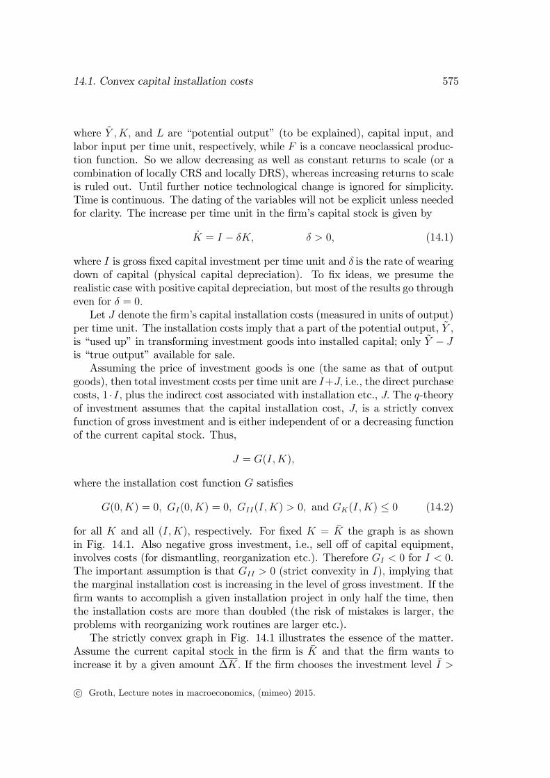
G(0, K) = 0, GI(0, K) = 0, GII(I,K) > 0, and GK(I,K) ≤ 0 (14.2)

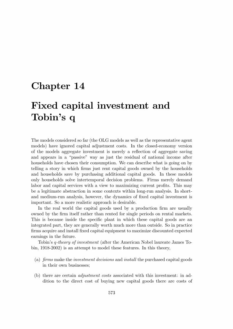
for all K and all (I,K), respectively. For fixed K = K the graph is as shownin Fig. 14.1. Also negative gross investment, i.e., sell off of capital equipment,involves costs (for dismantling, reorganization etc.). Therefore GI < 0 for I < 0.The important assumption is that GII > 0 (strict convexity in I), implying thatthe marginal installation cost is increasing in the level of gross investment. If thefirm wants to accomplish a given installation project in only half the time, thenthe installation costs are more than doubled (the risk of mistakes is larger, theproblems with reorganizing work routines are larger etc.).The strictly convex graph in Fig. 14.1 illustrates the essence of the matter.

Assume the current capital stock in the firm is K and that the firm wants toincrease it by a given amount ∆K. If the firm chooses the investment level I >



TOBIN’S Q

Figure 14.1: Installation costs as a function of gross investment when K = K.

0 per time unit in the time interval [t, t+ ∆t), then, in view of (14.1), ∆K≈ (I − δK)∆t. So it takes ∆t ≈ ∆K/(I − δK) units of time to accomplishthe desired increase ∆K. If, however, the firm slows down the adjustment andinvests only half of I per time unit, then it takes approximately twice as longtime to accomplish ∆K. Total costs of the two alternative courses of action areapproximately G(I , K)∆t and G(1

2I , K)2∆t, respectively (ignoring discounting

and assuming the initial increase in capital is small in relation to K). By drawinga few straight line segments in Fig. 14.1 the reader will be convinced that thelast-mentioned cost is smaller than the first-mentioned due to strict convexity ofinstallation costs (see Exercise 14.1). Haste is waste.

On the other hand, there are of course limits to how slow the adjustmentto the desired capital stock should be. Slower adjustment means postponementof the potential benefits of a higher capital stock. So the firm faces a trade-offbetween fast adjustment to the desired capital stock and low adjustment costs.

In addition to the strict convexity of G with respect to I, (14.2) imposesthe condition GK(I,K) ≤ 0. Indeed, it often seems realistic to assume thatGK(I,K) < 0 for I 6= 0. A given amount of investment may require morereorganization in a small firm than in a large firm (size here being measuredby K). When installing a new machine, a small firm has to stop productionaltogether, whereas a large firm can to some extent continue its production byshifting some workers to another production line. A further argument is thatthe more a firm has invested historically, the more experienced it is now. So,for a given I today, the associated installation costs are lower, given a largeraccumulated K.



14.1.1 The decision problem of the firm

In the absence of tax distortions, asymmetric information, and problems withenforceability of financial contracts, the Modigliani-Miller theorem (Modiglianiand Miller, 1958) says that the financial structure of the firm is both indeter-minate and irrelevant for production decisions (see Appendix A). Although theconditions required for this theorem are very idealized, the q-theory of investmentaccepts them because they allow the analyst to concentrate on the productionaspects in a first approach.With the output good as unit of account, let the operating cash flow (the net

payment stream to the firm before interest payments on debt, if any) at time tbe denoted Rt (for “receipts”). Then

Rt ≡ F (Kt, Lt)−G(It, Kt)− wtLt − It, (14.3)

where wt is the wage per unit of labor at time t. As mentioned, the installationcost G(It, Kt) implies that a part of production, F (Kt, Lt), is used up in trans-forming investment goods into installed capital; only the difference F (Kt, Lt) −G(It, Kt) is available for sale.We ignore uncertainty and assume the firm is a price taker. The interest rate

is rt, which we assume to be positive, at least in the long run. The decisionproblem, as seen from time 0, is to choose a plan (Lt, It)

∞t=0 so as to maximize the

firm’s market value, i.e., the present value of the future stream of expected cashflows:

max(Lt,It)∞t=0

V0 =

∫ ∞0

Rte−∫ t0 rsdsdt s.t. (14.3) and (14.4)

Lt ≥ 0, It free (i.e., no restriction on It), (14.5)

Kt = It − δKt, K0 > 0 given, (14.6)

Kt ≥ 0 for all t. (14.7)

There is no specific terminal condition but we have posited the feasibility condi-tion (14.7) saying that the firm can never have a negative capital stock.1

In the previous chapters the firm was described as solving a series of staticprofit maximization problems. Such a description is no longer valid, however,when there is dependence across time, as is the case here. When installation

1It is assumed that wt is a piecewise continuous function. At points of discontinuity (ifany) in investment, we will consider investment to be a right-continuous function of time.That is, It0 = limt→t+0

It. Likewise, at such points of discontinuity, by the “time derivative”

of the corresponding state variable, K, we mean the right-hand time derivative, i.e., Kt0 =limt→t+0

(Kt − Kt0)/(t − t0). Mathematically, these conventions are inconsequential, but theyhelp the intuition.



TOBIN’S Q

costs are present, current decisions depend on the expected future circumstances.The firmmakes a plan for the whole future so as to maximize the value of the firm,which is what matters for the owners. This is the general neoclassical hypothesisabout firms’behavior. As shown in Appendix A, when strictly convex installationcosts or similar dependencies across time are absent, then value maximization isequivalent to solving a sequence of static profit maximization problems, and weare back in the previous chapters’description.To solve the problem (14.4) − (14.7), where Rt is given by (14.3), we apply

the Maximum Principle. The problem has two control variables, L and I, andone state variable, K. We set up the current-value Hamiltonian:

H(K,L, I, q, t) ≡ F (K,L)− wL− I −G(I,K) + q(I − δK), (14.8)

where q (to be interpreted economically below) is the adjoint variable associatedwith the dynamic constraint (14.6). For each t ≥ 0 we maximize H w.r.t. thecontrol variables. Thus, ∂H/∂L = FL(K,L)− w = 0, i.e.,

FL(K,L) = w; (14.9)

and ∂H/∂I = −1−GI(I,K) + q = 0, i.e.,

1 +GI(I,K) = q. (14.10)

Next, we partially differentiateH w.r.t. the state variable and set the result equalto rq − q, where r is the discount rate in (14.4):

∂H

∂K= FK(K,L)−GK(I,K)− qδ = rq − q. (14.11)

Then, the Maximum Principle says that for an interior optimal path (Kt, Lt, It)there exists an adjoint variable q, which is a continuous function of t, written qt,such that for all t ≥ 0 the conditions (14.9), (14.10), and (14.11) hold and thetransversality condition

limt→∞

Ktqte−∫ t0 rsds = 0 (14.12)

is satisfied.The optimality condition (14.9) is the usual employment condition equalizing

the marginal product of labor to the real wage. In the present context withstrictly convex capital installation costs, this condition attains a distinct role aslabor will in the short run be the only variable input. This is because the strictlyconvex capital installation costs imply that the firm’s installed capital in theshort run is a quasi-fixed production factor. So, effectively there are diminishingreturns (equivalent with rising marginal costs) in the short run even though theproduction function might have CRS.



The left-hand side of (14.10) gives the cost of acquiring one extra unit ofinstalled capital at time t (the sum of the cost of buying the marginal investmentgood and the cost of its installation). That is, the left-hand side is the marginalcost, MC, of increasing the capital stock in the firm. Since (14.10) is a necessarycondition for optimality, the right-hand side of (14.10) must be the marginalbenefit, MB, of increasing the capital stock. Hence, qt represents the value tothe optimizing firm of having one more unit of (installed) capital at time t. Toput it differently: the adjoint variable qt can be interpreted as the shadow price(measured in current output units) of capital along the optimal path.2

As to the interpretation of the differential equation (14.11), a condition foroptimality must be that the firm acquires capital up to the point where the“marginal productivity of capital”, FK −GK , equals “capital costs”, rtqt + (δqt−qt); the first term in this expression represents interest costs and the secondeconomic depreciation. In (14.11) the “marginal productivity of capital”appearsas FK−GK , because we should take into account the potential reduction, −GK , ofinstallation costs in the next instant brought about by the marginal unit of alreadyinstalled capital. The shadow price qt appears as the “overall”price at which thefirm can buy and sell the marginal unit of installed capital. In fact, in view of qt =1+GI(Kt, Lt) along the optimal path (from (14.10)), qt measures, approximately,both the “overall” cost increase associated with increasing investment by oneunit and the “overall”cost saving associated with decreasing investment by oneunit. In the first case the firm not only has to pay one extra unit of accountin the investment goods market but must also bear an installation cost equal toGI(Kt, Lt), thereby in total investing qt units of account. And in the second casethe firm recovers qt by saving both on installation costs and purchases in theinvestment goods market. Continuing along this line of thought, by reordering in(14.11) we get the “no-arbitrage”condition

FK −GK − δq + q

q= r, (14.13)

saying that along the optimal path the rate of return on the marginal unit ofinstalled capital must equal the interest rate.The transversality condition (14.12) says that the present value of the capital

stock “left over”at infinity must be zero. That is, the capital stock should notin the long run grow too fast, given the evolution of its discounted shadow price.In addition to necessity of (14.12) it can be shown3 that the discounted shadow

2Recall that a shadow price, measured in some unit of account, of a good, from the point ofview of the buyer, is the maximum number of units of account that he or she is willing to offerfor one extra unit of the good.

3See Appendix B.



TOBIN’S Q

price itself in the far future must along an optimal path be asymptotically nil,i.e.,

limt→∞

qte−∫ t0 rsds = 0. (14.14)

If along the optimal path, Kt grows without bound, then not only must (14.14)hold but, in view of (14.12), the discounted shadow price must in the long runapproach zero faster than Kt grows. Intuitively, otherwise the firm would be“over-accumulating”. The firm would gain by reducing the capital stock “leftover” for eternity (which is like“money left on the table”), since reducing theultimate investment and installation costs would raise the present value of thefirm’s expected cash flow.In connection with (14.10) we claimed that qt can be interpreted as the shadow

price (measured in current output units) of capital along the optimal path. Aconfirmation of this interpretation is obtained by solving the differential equation(14.11). Indeed, multiplying by e−

∫ t0 (rs+δ)ds on both sides of (14.11), we get by

integration and application of (14.14),4

qt =

∫ ∞t

[FK(Kτ , Lτ )−GK(Iτ , Kτ )] e−∫ τt (rs+δ)dsdτ . (14.15)

The right-hand side of (14.15) is the present value, as seen from time t, of expectedfuture increases of the firm’s cash-flow that would result if one extra unit ofcapital were installed at time t; indeed, FK(Kτ , Lτ ) is the direct contributionto output of one extra unit of capital, while −GK(Iτ , Kτ ) ≥ 0 represents thepotential reduction of installation costs in the next instant brought about by themarginal unit of installed capital. However, future increases of cash-flow shouldbe discounted at a rate equal to the interest rate plus the capital depreciationrate; from one extra unit of capital at time t there are only e−δ(τ−t) units left attime τ .To concretize our interpretation of qt as representing the value to the opti-

mizing firm at time t of having one extra unit of installed capital, let us makea thought experiment. Assume that a extra units of installed capital at time tdrops down from the sky. At time τ > t there are a · e−δ(τ−t) units of these stillin operation so that the stock of installed capital is

K ′τ = Kτ + a · e−δ(τ−t), (14.16)

where Kτ denotes the stock of installed capital as it would have been withoutthis “injection”. Now, in (14.3) replace t by τ and consider the optimizing firm’s

4For details, see Appendix A.



cash-flow Rτ as a function of (Kτ , Lτ , Iτ , τ , t, a). Taking the partial derivative ofRτ w.r.t. a at the point (Kτ , Lτ , Iτ , τ , t, 0), we get

∂Rτ

∂a |a=0= [FK(Kτ , Lτ )−GK(Iτ , Kτ )] e

−δ(τ−t). (14.17)

Considering the value of the optimizing firm at time t as a function of installedcapital, Kt, and t itself, we denote this function V ∗(Kt, t). Then at any pointwhere V ∗ is differentiable, we have

∂V ∗(Kt, t)

∂Kt

=

∫ ∞t

(∂Rτ

∂a |a=0

)e−

∫ τt rsdsdτ

=

∫ ∞t

[FK(Kτ , Lτ )−GK(Iτ , Kτ )]e−∫ τt (rs+δ)dsdτ = qt (14.18)

when the firm moves along the optimal path. The second equality sign comesfrom (14.17) and the third is implied by (14.15). So the value of the adjointvariable, q, at time t equals the contribution to the firm’s maximized value of afictional marginal “injection” of installed capital at time t. This is just anotherway of saying that qt represents the benefit to the firm of the marginal unit ofinstalled capital along the optimal path.This story facilitates the understanding that the control variables at any point

in time should be chosen so that the Hamiltonian function is maximized. Therebyone maximizes the properly weighted sum of the current direct contribution to thecriterion function and the indirect contribution, which is the benefit (as measuredapproximately by qt∆Kt) of having a higher capital stock in the future.As we know, the Maximum Principle gives only necessary conditions for an

optimal path, not suffi cient conditions. We use the principle as a tool for findingcandidates for a solution. Having found in this way a candidate, one way to pro-ceed is to check whether Mangasarian’s suffi cient conditions are satisfied. Giventhe transversality condition (14.12) and the non-negativity of the state variable,K, the only additional condition to check is whether the Hamiltonian functionis jointly concave in the endogenous variables (here K, L, and I). If it is jointlyconcave in these variables, then the candidate is an optimal solution. Owingto concavity of F (K,L), inspection of (14.8) reveals that the Hamiltonian func-tion is jointly concave in (K,L, I) if −G(I, K) is jointly concave in (I,K). Thiscondition is equivalent to G(I,K) being jointly convex in (I,K), an assumptionallowed within the confines of (14.2); for example, G(I,K) = (1

2)βI2/K as well as

the simpler G(I,K) = (12)βI2 (where in both cases β > 0) will do. Thus, assum-

ing joint convexity of G(I,K), the first-order conditions and the transversalitycondition are not only necessary, but also suffi cient for an optimal solution.



TOBIN’S Q

14.1.2 The implied investment function

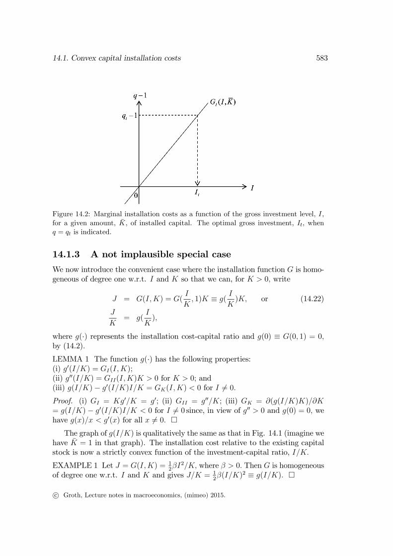
From condition (14.10) we can derive an investment function. Rewriting (14.10),we have that an optimal path satisfies

GI(It, Kt) = qt − 1. (14.19)

Combining this with the assumption (14.2) on the installation cost function, wesee that

It T 0 for qt T 1, respectively, (14.20)

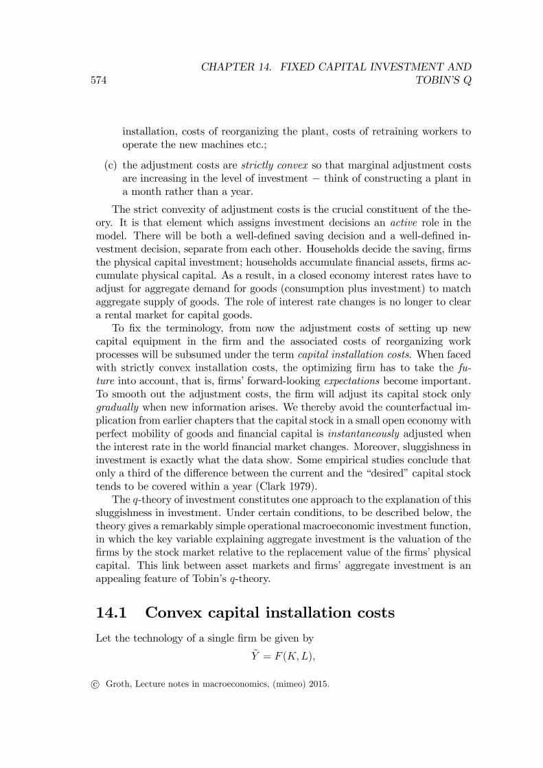
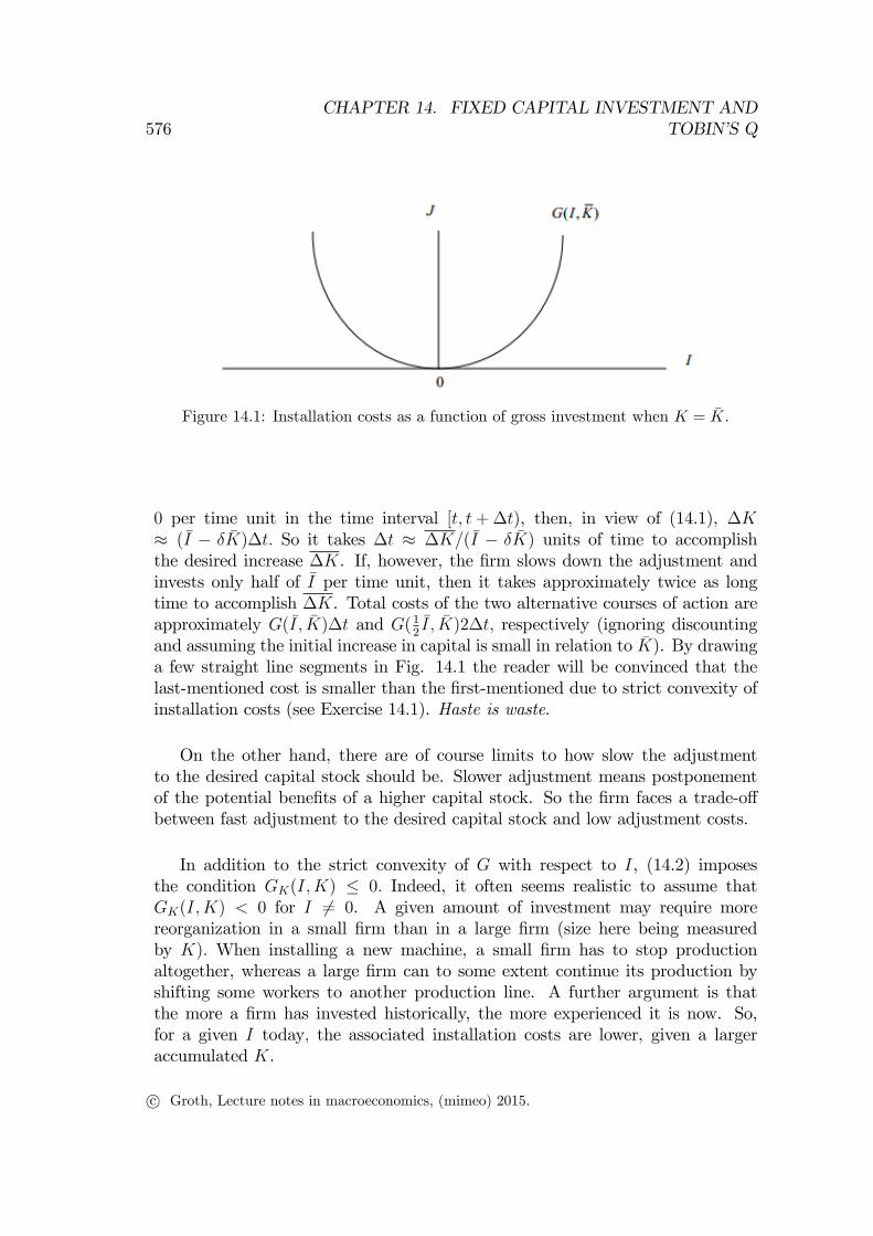
cf. Fig. 14.2.5 In view of GII 6= 0, (14.19) implicitly defines optimal investment,It, as a function of the shadow price, qt, and the state variable, Kt :

It =M(qt, Kt), (14.21)

where, in view of (14.20), M(1, Kt) = 0. By implicit differentiation w.r.t. qt andKt, respectively, in (14.19), we find

∂It∂qt

=1

GII(It, Kt)> 0, and

∂It∂Kt

= −GIK(It, Kt)

GII(It, Kt),

where the latter cannot be signed without further specification.It follows that optimal investment is an increasing function of the shadow

price of installed capital. In view of (14.20),M(1, K) = 0. Not surprisingly, theinvestment rule is: invest now, if and only if the value to the firm of the marginalunit of installed capital is larger than the price of the capital good (which is1, excluding installation costs). At the same time, the rule says that, becauseof the convex installation costs, invest only up to the point where the marginalinstallation cost, GI(It, Kt), equals qt − 1, cf. (14.19).Condition (14.21) shows the remarkable information content that the shadow

price qt has. As soon as qt is known (along with the current capital stock Kt),the firm can decide the optimal level of investment through knowledge of theinstallation cost function G alone (since, when G is known, so is in principle theinverse of GI w.r.t. I, the investment functionM). All the information about theproduction function, input prices, and interest rates now and in the future thatis relevant to the investment decision is summarized in one number, qt. The formof the investment function,M, depends only on the installation cost function G.These are very useful properties in theoretical and empirical analysis.

5From the assumptions made in (14.2), we only know that the graph of GI(I, K) is anupward-sloping curve going through the origin. Fig. 14.2 shows the special case where thiscurve happens to be linear.



Figure 14.2: Marginal installation costs as a function of the gross investment level, I,for a given amount, K, of installed capital. The optimal gross investment, It, whenq = qt is indicated.

14.1.3 A not implausible special case

We now introduce the convenient case where the installation function G is homo-geneous of degree one w.r.t. I and K so that we can, for K > 0, write

J = G(I,K) = G(I

K, 1)K ≡ g(

I

K)K, or (14.22)

J

K= g(

I

K),

where g(·) represents the installation cost-capital ratio and g(0) ≡ G(0, 1) = 0,by (14.2).

LEMMA 1 The function g(·) has the following properties:(i) g′(I/K) = GI(I,K);(ii) g′′(I/K) = GII(I,K)K > 0 for K > 0; and(iii) g(I/K)− g′(I/K)I/K = GK(I,K) < 0 for I 6= 0.

Proof. (i) GI = Kg′/K = g′; (ii) GII = g′′/K; (iii) GK = ∂(g(I/K)K)/∂K= g(I/K)− g′(I/K)I/K < 0 for I 6= 0 since, in view of g′′ > 0 and g(0) = 0, wehave g(x)/x < g′(x) for all x 6= 0. �The graph of g(I/K) is qualitatively the same as that in Fig. 14.1 (imagine we

have K = 1 in that graph). The installation cost relative to the existing capitalstock is now a strictly convex function of the investment-capital ratio, I/K.

EXAMPLE 1 Let J = G(I,K) = 12βI2/K, where β > 0. Then G is homogeneous

of degree one w.r.t. I and K and gives J/K = 12β(I/K)2 ≡ g(I/K). �



TOBIN’S Q

A further important property of (14.22) is that the cash-flow function in (14.3)becomes homogeneous of degree one w.r.t. K, L, and I in the “normal”case wherethe production function has CRS. This has two implications. First, Hayashi’stheorem applies (see below). Second, the q-theory can easily be incorporatedinto a model of economic growth.6

Does the hypothesis of linear homogeneity of the cash flow in K, L, and Imake economic sense? According to the replication argument it does. Suppose agiven firm has K units of installed capital and produces Y units of output withL units of labor. When at the same time the firm invests I units of accountin new capital, it obtains the cash flow R after deducting the installation costs,G(I,K). Then it makes sense to assume that the firm could do the same thing atanother place, hereby doubling its cash-flow. (Of course, owing to the possibilityof indivisibilities, this reasoning does not take us all the way to linear homogeneity.Moreover, the argument ignores that also land is a necessary input. As discussedin Chapter 2, the empirical evidence on linear homogeneity is mixed.)In view of (i) of Lemma 1, the linear homogeneity assumption for G allows us

to write (14.19) asg′(I/K) = q − 1. (14.23)

This equation defines the investment-capital ratio, I/K , as an implicit function,m, of q :

ItKt

= m(qt), where m(1) = 0 and m′ =1

g′′> 0, (14.24)

by implicit differentiation in (14.23). In this case q encompasses all informationthat is of relevance to the decision about the investment-capital ratio.In Example 1 above we have g(I/K) = 1

2β(I/K)2, in which case (14.23) gives

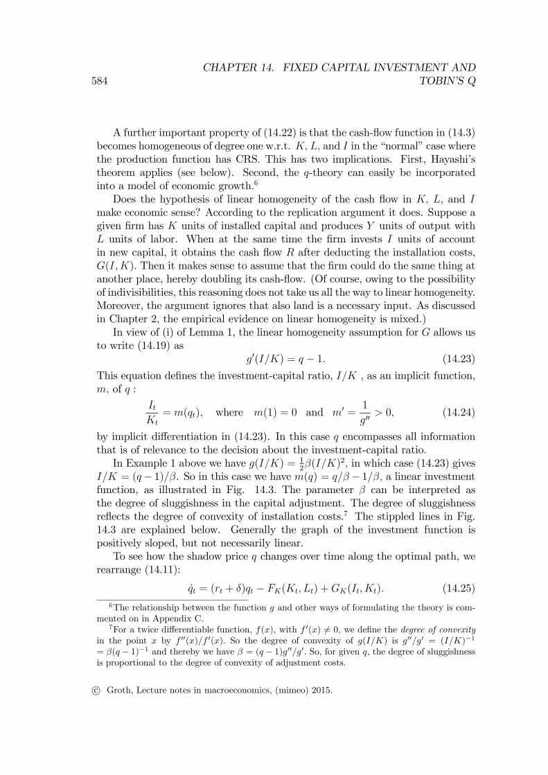
I/K = (q− 1)/β. So in this case we have m(q) = q/β − 1/β, a linear investmentfunction, as illustrated in Fig. 14.3. The parameter β can be interpreted asthe degree of sluggishness in the capital adjustment. The degree of sluggishnessreflects the degree of convexity of installation costs.7 The stippled lines in Fig.14.3 are explained below. Generally the graph of the investment function ispositively sloped, but not necessarily linear.To see how the shadow price q changes over time along the optimal path, we

rearrange (14.11):

qt = (rt + δ)qt − FK(Kt, Lt) +GK(It, Kt). (14.25)6The relationship between the function g and other ways of formulating the theory is com-

mented on in Appendix C.7For a twice differentiable function, f(x), with f ′(x) 6= 0, we define the degree of convexity

in the point x by f ′′(x)/f ′(x). So the degree of convexity of g(I/K) is g′′/g′ = (I/K)−1

= β(q − 1)−1 and thereby we have β = (q − 1)g′′/g′. So, for given q, the degree of sluggishnessis proportional to the degree of convexity of adjustment costs.



Figure 14.3: Optimal investment-capital ratio as a function of the shadow price ofinstalled capital when g(I/K) = 1

2β(I/K)2.

Recall that −GK(It, Kt) indicates how much lower the installation costs are asa result of the marginal unit of installed capital. In the special case (14.22) wehave from Lemma 1

GK(I,K) = g(I

K)− g′( I

K)I

K= g(m(q))− (q − 1)m(q),

using (14.24) and (14.23).

Inserting this into (14.25) gives

qt = (rt + δ)qt − FK(Kt, Lt) + g(m(qt))− (qt − 1)m(qt). (14.26)

This differential equation is very useful in macroeconomic analysis, as we willsoon see, cf. Fig. 14.4 below.

In a macroeconomic context, for steady state to achievable, gross investmentmust be large enough to match not only capital depreciation, but also growth inthe labor input. Otherwise a constant capital-labor ratio can not be sustained.That is, the investment-capital ratio, I/K, must be equal to the sum of thedepreciation rate and the growth rate of the labor force, i.e., δ+n. The level of qwhich is required to motivate such an investment-capital ratio is called q∗ in Fig.14.3.



TOBIN’S Q

14.2 Marginal q and average q

Our q above, determining investment, should be distinguished from what is usu-ally called Tobin’s q or average q. In a more general context, let pIt denotethe current purchase price (in terms of output units) per unit of the invest-ment good (before installment). Then Tobin’s q or average q, qat , is defined asqat ≡ Vt/(pItKt), that is, Tobin’s q is the ratio of the market value of the firm tothe replacement value of the firm in the sense of the “reacquisition value of thecapital goods before installment costs”(the top index “a”stands for “average”).In our simplified context we have pIt ≡ 1 (the price of the investment good is thesame as that of the output good). Therefore Tobin’s q can be written

qat ≡VtKt

=V ∗(Kt, t)

Kt

, (14.27)

where the equality holds for an optimizing firm. Conceptually this is differentfrom the firm’s internal shadow price on capital, i.e., what we have denoted qtin the previous sections. In the language of the q-theory of investment this qt isthe marginal q, representing the value to the firm of one extra unit of installedcapital relative to the price of un-installed capital equipment. The term marginalq is natural since along the optimal path, as a slight generalization of (14.18), wemust have qt = (∂V ∗/∂Kt)/pIt. Letting qmt (“m”for “marginal”) be an alternativesymbol for this qt, we have in our model above, where we consider the specialcase pIt ≡ 1,

qmt ≡ qt =∂V ∗

∂Kt

. (14.28)

The two concepts, average q and marginal q, have not always been clearly dis-tinguished in the literature. What is directly relevant to the investment decisionis marginal q. Indeed, the analysis above showed that optimal investment is anincreasing function of qm. Further, the analysis showed that a “critical”value ofqm is 1 and that only if qm > 1, is positive gross investment warranted.The importance of qa is that it can be measured empirically as the ratio of the

sum of the share market value of the firm and its debt to the current acquisitionvalue of its total capital before installment. Since qm is much harder to measurethan qa, it is important to know the relationship between qm and qa. Fortunately,we have a simple theorem giving conditions under which qm = qa.

THEOREM (Hayashi, 1982) Assume the firm is a price taker, that the productionfunction F is jointly concave in (K,L), and that the installation cost function Gis jointly convex in (I,K).8 Then, along an optimal path we have:

8That is, in addition to (14.2), we assume GKK ≥ 0 and GIIGKK −G2IK ≥ 0. The specifi-cation in Example 1 above satisfies this.


14.3. Applications 587

(i) qmt = qat for all t ≥ 0, if F and G are homogeneous of degree 1.(ii) qmt < qat for all t, if F is strictly concave in (K, L) and/or G is strictly

convex in (I, K).Proof. See Appendix D.

The assumption that the firm is a price taker may, of course, seem critical.The Hayashi theorem has been generalized, however. Also a monopolistic firm,facing a downward-sloping demand curve and setting its own price, may have acash flow which is homogeneous of degree one in the three variables K,L, and I.If so, then the condition qmt = qat for all t ≥ 0 still holds (Abel 1990). Abel andEberly (1994) present further generalizations.In any case, when qm is approximately equal to (or just proportional to)

qa, the theory gives a remarkably simple operational investment function, I =m(qa)K, cf. (14.24). At the macro level we interpret qa as the market valuationof the firms relative to the replacement value of their total capital stock. Thismarket valuation is an indicator of the expected future earnings potential of thefirms. Under the conditions in (i) of the Hayashi theorem the market valuationalso indicates the marginal earnings potential of the firms, hence, it becomes adeterminant of their investment. This establishment of a relationship between thestock market and firms’aggregate investment is the basic point in Tobin (1969).

14.3 Applications

Capital installation costs in a closed economy

Allowing for convex capital installation costs in the economy has far-reachingimplications for the causal structure of a model of a closed economy. Investmentdecisions attain an active role in the economy and forward-looking expectationsbecome important for these decisions. Expected future market conditions and an-nounced future changes in corporate taxes and depreciation allowance will affectfirms’investment already today.The essence of the matter is that current and expected future interest rates

have to adjust for aggregate saving to equal aggregate investment, that is, for theoutput and asset markets to clear. Given full employment (Lt = Lt), the outputmarket clears when

F (Kt, Lt)−G(It, Kt) = value added ≡ GDPt = Ct + It,

where Ct is determined by the intertemporal utility maximization of the forward-looking households, and It is determined by the intertemporal value maximizationof the forward-looking firms facing strictly convex installation costs. Like in thedetermination of Ct, current and expected future interest rates now also matter



TOBIN’S Q

for the determination of It. This is the first time in this book where clearing in theoutput market is assigned an active role. In the earlier models investment was justa passive reflection of household saving. Desired investment was automaticallyequal to the residual of national income left over after consumption decisions hadtaken place. Nothing had to adjust to clear the output market, neither interestrates nor output. In contrast, in the present framework adjustments in interestrates and/or the output level are needed for the continuous clearing in the outputmarket and these adjustments are decisive for the macroeconomic dynamics.In actual economies there may of course exist “secondary markets” for used

capital goods and markets for renting capital goods owned by others. In view ofinstallation costs and similar, however, shifting capital goods from one plant toanother is generally costly. Therefore the turnover in that kind of markets tendsto be limited and there is little underpinning for the earlier models’suppositionthat the current interest rate should be tied down by a requirement that suchmarkets clear.In for instance Abel and Blanchard (1983) a Ramsey-style model integrating

the q-theory of investment is presented. The authors study the two-dimensionalgeneral equilibrium dynamics resulting from the adjustment of current and ex-pected future (short-term) interest rates needed for the output market to clear.Adjustments of the whole structure of interest rates (the yield curve) take placeand constitute the equilibrating mechanism in the output and asset markets.By having output market equilibrium playing this role in the model, a first

step is taken towards medium- and short-run macroeconomic theory. We takefurther steps in later chapters, by allowing imperfect competition and nominalprice rigidities to enter the picture. Then the demand side gets an active roleboth in the determination of q (and thereby investment) and in the determinationof aggregate output and employment. This is what Keynesian theory (old andnew) deals with.In the remainder of this chapter we will still assume perfect competition in all

markets including the labor market. In this sense we will stay within the neoclas-sical framework (supply-dominated models) where, by instantaneous adjustmentof the real wage, labor demand continuously matches labor supply. The nexttwo subsections present examples of how Tobin’s q-theory of investment can beintegrated into the neoclassical framework. To avoid the more complex dynamicsarising in a closed economy, we shift the focus to a small open economy. Thisallows concentrating on a dynamic system with an exogenous interest rate.

A small open economy with capital installation costs

By introducing convex capital installation costs in a model of a small open econ-omy (SOE), we avoid the counterfactual outcome that the capital stock adjusts



instantaneously when the interest rate in the world financial market changes.In the standard neoclassical growth model for a small open economy, withoutconvex capital installation costs, a rise in the interest rate leads immediately toa complete adjustment of the capital stock so as to equalize the net marginalproductivity of capital to the new higher interest rate. Moreover, in that modelexpected future changes in the interest rate or in corporate taxes and deprecia-tion allowances do not trigger an investment response until these changes actuallyhappen. In contrast, when convex installation costs are present, expected futurechanges tend to influence firms’investment already today.We assume:

1. Perfect mobility across borders of goods and financial capital.

2. Domestic and foreign financial claims are perfect substitutes.

3. No mobility across borders of labor.

4. Labor supply is inelastic and constant and there is no technological progress.

5. The capital installation cost function G(I,K) is homogeneous of degree 1.

In this setting the SOE faces an exogenous interest rate, r, given from theworld financial market. We assume r is a positive constant. The aggregate pro-duction function, F (K,L), is neoclassical and concave as in the previous sections.With L > 0 denoting the constant labor supply, continuous clearing in the labormarket under perfect competition gives Lt = L for all t ≥ 0 and

wt = FL(Kt, L) ≡ w(Kt). (14.29)

At any time t, Kt is predetermined in the sense that due to the convex installationcosts, changes in K take time. Thus (14.29) determines the market real wage wt.To pin down the evolution of the economy, we now derive two coupled differ-

ential equations in K and q. Inserting (14.24) into (14.6) gives

Kt = (m(qt)− δ)Kt, K0 > 0 given. (14.30)

As to the dynamics of q, we have (14.26). Since the capital installation costfunction G(I,K) is assumed to be homogeneous of degree 1, point (iii) of Lemma1 applies and we can write (14.26) as

qt = (r + δ)qt − FK(Kt, L) + g(m(qt))− (qt − 1)m(qt). (14.31)

As r and L are exogenous, the capital stock, K, and its shadow price, q, arethe only endogenous variables in the differential equations (14.30) and (14.31).



TOBIN’S Q

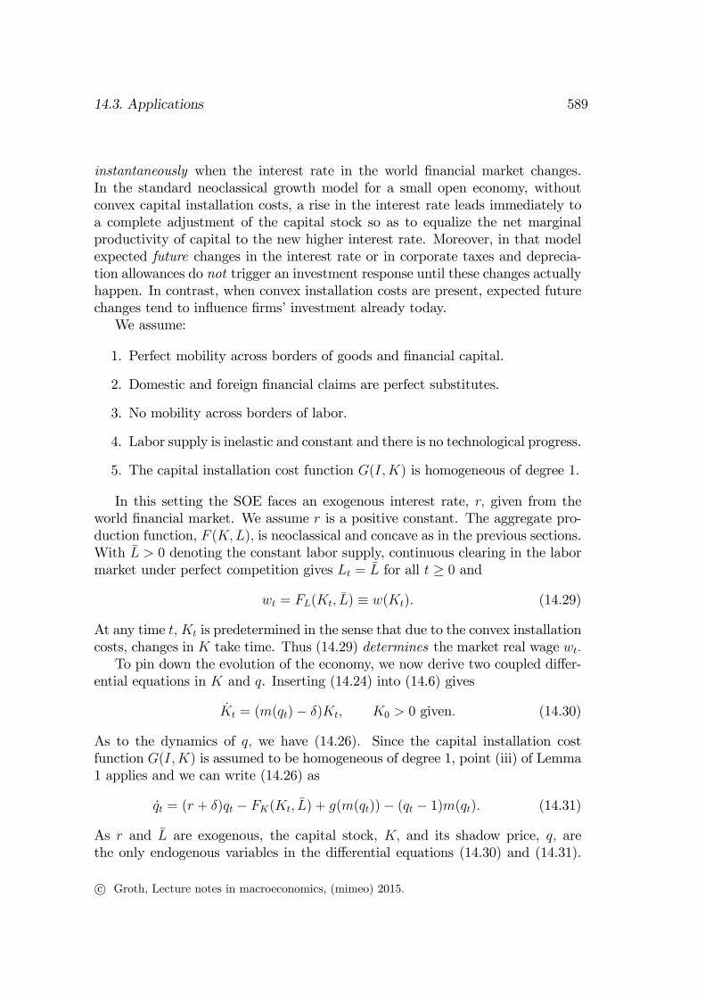
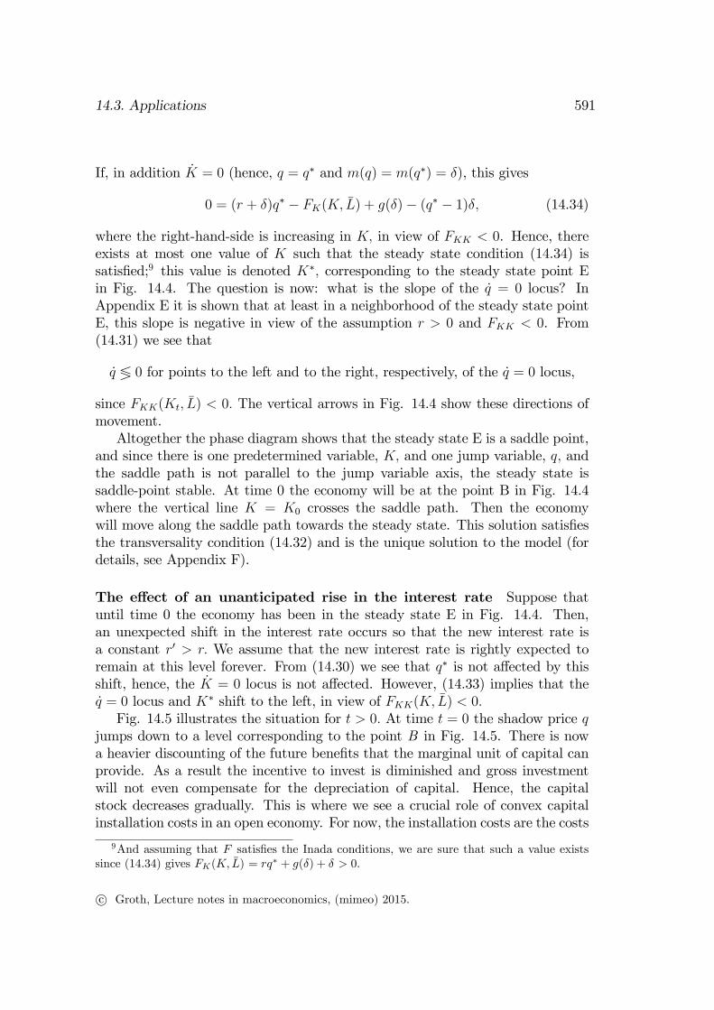
Figure 14.4: Phase diagram for investment dynamics in a small open economy (a casewhere δ > 0).

In addition, we have an initial condition for K and a necessary transversalitycondition involving q, namely

limt→∞

Ktqte−rt = 0. (14.32)

Fig. 14.4 shows the phase diagram for these two coupled differential equations.Let q∗ be defined as the value of q satisfying the equationm(q) = δ. Sincem′ > 0,q∗ is unique. Suppressing for convenience the explicit time subscripts, we thenhave

K = 0 for m(q) = δ, i.e., for q = q∗.

As δ > 0, we have q∗ > 1. This is so because also mere reinvestment to offsetcapital depreciation requires an incentive, namely that the marginal value tothe firm of replacing worn-out capital is larger than the purchase price of theinvestment good (since the installation cost must also be compensated). From(14.30) is seen that

K ≷ 0 for m(q) ≷ δ, respectively, i.e., for q ≷ q∗, respectively,

cf. the horizontal arrows in Fig. 14.4.From (14.31) we have

q = 0 for 0 = (r + δ)q − FK(K, L) + g(m(q))− (q − 1)m(q). (14.33)



If, in addition K = 0 (hence, q = q∗ and m(q) = m(q∗) = δ), this gives

0 = (r + δ)q∗ − FK(K, L) + g(δ)− (q∗ − 1)δ, (14.34)

where the right-hand-side is increasing in K, in view of FKK < 0. Hence, thereexists at most one value of K such that the steady state condition (14.34) issatisfied;9 this value is denoted K∗, corresponding to the steady state point Ein Fig. 14.4. The question is now: what is the slope of the q = 0 locus? InAppendix E it is shown that at least in a neighborhood of the steady state pointE, this slope is negative in view of the assumption r > 0 and FKK < 0. From(14.31) we see that

q ≶ 0 for points to the left and to the right, respectively, of the q = 0 locus,

since FKK(Kt, L) < 0. The vertical arrows in Fig. 14.4 show these directions ofmovement.Altogether the phase diagram shows that the steady state E is a saddle point,

and since there is one predetermined variable, K, and one jump variable, q, andthe saddle path is not parallel to the jump variable axis, the steady state issaddle-point stable. At time 0 the economy will be at the point B in Fig. 14.4where the vertical line K = K0 crosses the saddle path. Then the economywill move along the saddle path towards the steady state. This solution satisfiesthe transversality condition (14.32) and is the unique solution to the model (fordetails, see Appendix F).

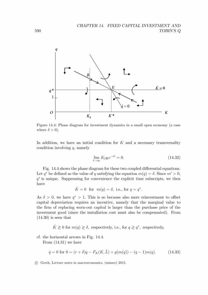
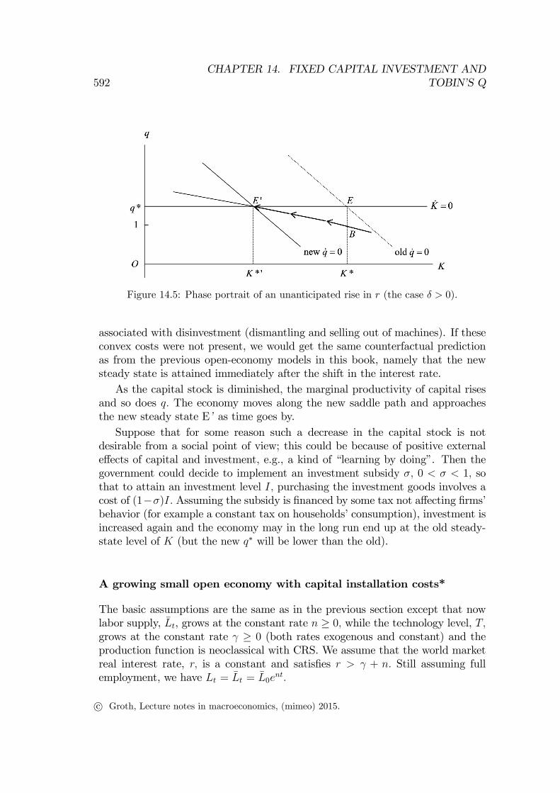
The effect of an unanticipated rise in the interest rate Suppose thatuntil time 0 the economy has been in the steady state E in Fig. 14.4. Then,an unexpected shift in the interest rate occurs so that the new interest rate isa constant r′ > r. We assume that the new interest rate is rightly expected toremain at this level forever. From (14.30) we see that q∗ is not affected by thisshift, hence, the K = 0 locus is not affected. However, (14.33) implies that theq = 0 locus and K∗ shift to the left, in view of FKK(K, L) < 0.Fig. 14.5 illustrates the situation for t > 0. At time t = 0 the shadow price q

jumps down to a level corresponding to the point B in Fig. 14.5. There is nowa heavier discounting of the future benefits that the marginal unit of capital canprovide. As a result the incentive to invest is diminished and gross investmentwill not even compensate for the depreciation of capital. Hence, the capitalstock decreases gradually. This is where we see a crucial role of convex capitalinstallation costs in an open economy. For now, the installation costs are the costs

9And assuming that F satisfies the Inada conditions, we are sure that such a value existssince (14.34) gives FK(K, L) = rq∗ + g(δ) + δ > 0.



TOBIN’S Q

Figure 14.5: Phase portrait of an unanticipated rise in r (the case δ > 0).

associated with disinvestment (dismantling and selling out of machines). If theseconvex costs were not present, we would get the same counterfactual predictionas from the previous open-economy models in this book, namely that the newsteady state is attained immediately after the shift in the interest rate.As the capital stock is diminished, the marginal productivity of capital rises

and so does q. The economy moves along the new saddle path and approachesthe new steady state E’ as time goes by.Suppose that for some reason such a decrease in the capital stock is not

desirable from a social point of view; this could be because of positive externaleffects of capital and investment, e.g., a kind of “learning by doing”. Then thegovernment could decide to implement an investment subsidy σ, 0 < σ < 1, sothat to attain an investment level I, purchasing the investment goods involves acost of (1−σ)I. Assuming the subsidy is financed by some tax not affecting firms’behavior (for example a constant tax on households’consumption), investment isincreased again and the economy may in the long run end up at the old steady-state level of K (but the new q∗ will be lower than the old).

A growing small open economy with capital installation costs*

The basic assumptions are the same as in the previous section except that nowlabor supply, Lt, grows at the constant rate n ≥ 0, while the technology level, T,grows at the constant rate γ ≥ 0 (both rates exogenous and constant) and theproduction function is neoclassical with CRS. We assume that the world marketreal interest rate, r, is a constant and satisfies r > γ + n. Still assuming fullemployment, we have Lt = Lt = L0e

nt.



In this setting the production function on intensive form is useful:

Y = F (K,T L) = F (K

TL, 1)TL ≡ f(k)TL,

where k ≡ K/(TL) and f satisfies f ′ > 0 and f ′′ < 0. Still assuming perfectcompetition, the market-clearing real wage at time t is determined as

wt = F2(Kt, TtLt)Tt =[f(kt)− ktf ′(kt)

]Tt ≡ w(kt)Tt,

where both kt and Tt are predetermined. By log-differentiation of k ≡ K/(TL)

w.r.t. time we get·kt/kt = Kt/Kt − (γ + n). Substituting (14.30), we get

·kt = [m(qt)− (δ + γ + n)] kt. (14.35)

The change in the shadow price of capital is now described by

qt = (r + δ)qt − f ′(kt) + g(m(qt))− (qt − 1)m(qt), (14.36)

from (14.26). In addition, the transversality condition,

limt→∞

ktqte−(r−γ−n)t = 0, (14.37)

must hold.The differential equations (14.35) and (14.36) constitute our new dynamic

system. Fig. 14.6 shows the phase diagram, which is qualitatively similar to thatin Fig. 14.4. We have

·k = 0 for m(q) = δ + γ + n, i.e., for q = q∗,

where q∗ now is defined by the requirement m(q∗) = δ+ γ+n. Notice, that whenγ+n > 0, we get a larger steady state value q∗ than in the previous section. Thisis so because now a higher investment-capital ratio is required for a steady stateto be possible. Moreover, the transversality condition (14.12) is satisfied in thesteady state.From (14.36) we see that q = 0 now requires

0 = (r + δ)q − f ′(k) + g(m(q))− (q − 1)m(q).

If, in addition·k = 0 (hence, q = q∗ and m(q) = m(q∗) = δ + γ + n), this gives

0 = (r + δ)q∗ − f ′(k) + g(δ + γ + n)− (q∗ − 1)(δ + γ + n).



TOBIN’S Q

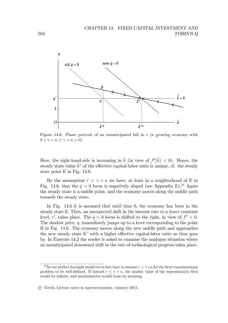
Figure 14.6: Phase portrait of an unanticipated fall in r (a growing economy withδ + γ + n ≥ γ + n > 0).

Here, the right-hand-side is increasing in k (in view of f ′′(k) < 0). Hence, thesteady state value k∗ of the effective capital-labor ratio is unique, cf. the steadystate point E in Fig. 14.6.

By the assumption r > γ + n we have, at least in a neighborhood of E inFig. 14.6, that the q = 0 locus is negatively sloped (see Appendix E).10 Againthe steady state is a saddle point, and the economy moves along the saddle pathtowards the steady state.

In Fig. 14.6 it is assumed that until time 0, the economy has been in thesteady state E. Then, an unexpected shift in the interest rate to a lower constantlevel, r′, takes place. The q = 0 locus is shifted to the right, in view of f ′′ < 0.The shadow price, q, immediately jumps up to a level corresponding to the pointB in Fig. 14.6. The economy moves along the new saddle path and approachesthe new steady state E’ with a higher effective capital-labor ratio as time goesby. In Exercise 14.2 the reader is asked to examine the analogue situation wherean unanticipated downward shift in the rate of technological progress takes place.

10In our perfect foresight model we in fact have to assume r > γ+n for the firm’s maximizationproblem to be well-defined. If instead r ≤ γ + n, the market value of the representative firmwould be infinite, and maximization would loose its meaning.


14.4. Concluding remarks 595

14.4 Concluding remarks

Tobin’s q-theory of investment gives a remarkably simple operational macroeco-nomic investment function, in which the key variable explaining aggregate invest-ment is the valuation of the firms by the stock market relative to the replacementvalue of the firms’physical capital. This link between asset markets and firms’aggregate investment is an appealing feature of Tobin’s q-theory.When faced with strictly convex installation costs, the firm has to take the

future into account to invest optimally. Therefore, the firm’s expectations be-come important. Owing to the strictly convex installation costs, the firm adjustsits capital stock only gradually when new information arises. This investmentsmoothing is analogue to consumption smoothing.By incorporating these features, Tobin’s q-theory helps explaining the slug-

gishness in investment we see in the empirical data. And the theory avoids thecounterfactual outcome from earlier chapters that the capital stock in a smallopen economy with perfect mobility of goods and financial capital is instanta-neously adjusted when the interest rate in the world market changes. So thetheory takes into account the time lags in capital adjustment in real life, a fea-ture which may, perhaps, be abstracted from in long-run analysis and models ofeconomic growth, but not in short- and medium-run analysis.Many econometric tests of the q theory of investment have been made, often

with quite critical implications. Movements in qa, even taking account of changesin taxation, seemed capable of explaining only a minor fraction of the movementsin investment. And the estimated equations relating fixed capital investmentto qa typically give strong auto-correlation in the residuals. Other variables, inparticular availability of current corporate profits for internal financing, seemto have explanatory power independently of qa (see Abel 1990, Chirinko 1993,Gilchrist and Himmelberg, 1995). So there is reason to be somewhat scepticaltowards the notion that all information of relevance for the investment decisionis reflected by the market valuation of firms. This throws doubt on the basicassumption in Hayashi’s theorem or its generalization, the assumption that firms’cash flow tends to be homogeneous of degree one w.r.t. K, L, and I.Going outside the model, there are further circumstances relaxing the link

between qa and investment. In the real world with many production sectors,physical capital is heterogeneous. If for example a sharp unexpected rise in theprice of energy takes place, a firm with energy-intensive technology will loose inmarket value. At the same time it has an incentive to invest in energy-savingcapital equipment. Hence, we might observe a fall in qa at the same time asinvestment increases.Imperfections in credit markets are ignored by the model. Their presence



TOBIN’S Q

further loosens the relationship between qa and investment and may help explainthe observed positive correlation between investment and corporate profits.

We might also question that capital installation costs really have the hy-pothesized strictly convex form. It is one thing that there are costs associatedwith installation, reorganizing and retraining etc., when new capital equipmentis procured. But should we expect these costs to be strictly convex in the vol-ume of investment? To think about this, let us for a moment ignore the roleof the existing capital stock. Hence, we write total installation costs J = G(I)with G(0) = 0. It does not seem problematic to assume G′(I) > 0 for I > 0.The question concerns the assumption G′′(I) > 0. According to this assumptionthe average installation cost G(I)/I must be increasing in I.11 But against thisspeaks the fact that capital installation may involve indivisibilities, fixed costs,acquisition of new information etc. All these features tend to imply decreasingaverage costs. In any case, at least at the microeconomic level one should ex-pect unevenness in the capital adjustment process rather than the above smoothadjustment.

Because of the mixed empirical success of the convex installation cost hypoth-esis other theoretical approaches that can account for sluggish and sometimesnon-smooth and lumpy capital adjustment have been considered: uncertainty,investment irreversibility, indivisibility, or financial problems due to bankruptcycosts (Nickell 1978, Zeira 1987, Dixit and Pindyck 1994, Caballero 1999, Adda andCooper 2003). These approaches notwithstanding, it turns out that the q-theoryof investment has recently been somewhat rehabilitated from both a theoreticaland an empirical point of view. At the theoretical level Wang and Wen (2010)show that financial frictions in the form of collateralized borrowing at the firmlevel can give rise to strictly convex adjustment costs at the aggregate level yetat the same time generate lumpiness in plant-level investment. For large firms,unlikely to be much affected by financial frictions, Eberly et al. (2008) find thatthe theory does a good job in explaining investment behavior.

In any case, the q-theory of investment is in different versions widely usedin short- and medium-run macroeconomics because of its simplicity and the ap-pealing link it establishes between asset markets and firms’investment. And theq-theory has also had an important role in studies of the housing market and therole of housing prices for household wealth and consumption, a theme to whichwe return in the next chapter.

11Indeed, for I 6= 0 we have d[G(I)/I]/dI = [IG′(I)−G(I)]/I2 > 0, when G is strictly convex(G′′ > 0) and G(0) = 0.


14.5. Literature notes 597

14.5 Literature notes

A first sketch of the q-theory of investment is contained in Tobin (1969). Lateradvances of the theory took place through the contributions of Hayashi (1982)and Abel (1990).Both the Ramsey model and the Blanchard OLG model for a closed market

economy may be extended by adding strictly convex capital installation costs, seeAbel and Blanchard (1983) and Lim and Weil (2003). Adding a public sector,such a framework is useful for the study of how different subsidies, taxes, anddepreciation allowance schemes affect investment in physical capital as well ashousing, see, e.g., Summers (1981), Abel and Blanchard (1983), and Dixit (1990).Groth andMadsen (2013) study medium-termfluctuations arising in a Ramsey-

Tobin’s q framework when extended by sluggishness in real wage adjustments.

14.6 Appendix

A.When value maximization is - and is not - equivalent with continuousstatic profit maximization

For the idealized case where tax distortions, asymmetric information, and prob-lems with enforceability of financial contracts are absent, the Modigliani-Millertheorem (Modigliani and Miller, 1958) says that the financial structure of the firmis both indeterminate and irrelevant for production outcomes. Considering thefirm described in Section 14.1, the implied separation of the financing decisionfrom the production and investment decision can be exposed in the following way.

Simple version of the Modigliani-Miller theorem Although the theoremallows for risk, we here ignore risk. Let the real debt of the firm be denoted Bt

and the real dividends, Xt. We then have the accounting relationship

Bt = Xt − (F (Kt, Lt)−G(It, Kt)− wtLt − It − rtBt) .

A positive Xt represents dividends in the usual meaning (payout to the ownersof the firm), whereas a negative Xt can be interpreted as emission of new sharesof stock. Since we assume perfect competition, the time path of wt and rt isexogenous to the firm.We first consider the firm’s combined financing and production-investment

problem, which we call Problem I. We assume that those who own the firm attime 0 want it to maximize its net worth, i.e., the present value of expected future



TOBIN’S Q

dividends:

max(Lt,It,Xt)∞t=0

V0 =

∫ ∞0

Xte−∫ t0 rsdsdt s.t.

Lt ≥ 0, It free,

Kt = It − δKt, K0 > 0 given, Kt ≥ 0 for all t,

Bt = Xt − (F (Kt, Lt)−G(It, Kt)− wtLt − It − rtBt) ,

where B0 is given, (14.38)

limt→∞

Bte−∫ t0 rsds ≤ 0. (NPG)

The last constraint is a No-Ponzi-Game condition, saying that a positive debtshould in the long run at most grow at a rate which is less than the interest rate.In Section 14.1 we considered another problem, namely a separate investment-

production problem:

max(Lt,It)∞t=0

V0 =

∫ ∞0

Rte−∫ t0 rsdsdt s.t.,

Rt ≡ F (Kt, Lt)−G(It, Kt)− wtLt − It,Lt ≥ 0, It free,

Kt = It − δKt, K0 > 0 given, Kt ≥ 0 for all t.

Let this problem, where the financing aspects are ignored, be called ProblemII. When considering the relationship between Problem I and Problem II, thefollowing mathematical fact is useful.

LEMMA A1 Consider a continuous function a(t) and a differentiable functionf(t). Then∫ t1

t0

(f ′(t)− a(t)f(t))e−∫ tt0a(s)ds

dt = f(t1)e−∫ t1t0a(s)ds − f(t0).

Proof. Integration by parts from time t0 to time t1 yields∫ t1

t0

f ′(t)e−∫ tt0a(s)ds

dt = f(t)e−∫ tt0a(s)ds

∣∣t1t0 +

∫ t1

t0

f(t)a(t)e−∫ tt0a(s)ds

dt.

Hence, ∫ t1

t0

(f ′(t)− a(t)f(t))e−∫ tt0a(s)ds

dt

= f(t1)e−∫ t1t0a(s)ds − f(t0). �


14.6. Appendix 599

CLAIM 1 If (K∗t , B∗t , L

∗t , I∗t , X

∗t )∞t=0 is a solution to Problem I, then (K∗t , L

∗t , I∗t )∞t=0

is a solution to Problem II.

Proof. By (14.38) and the definition of Rt, Xt = Rt + Bt − rtBt so that

V0 =

∫ ∞0

Xte−∫ t0 rsdsdt = V0 +

∫ ∞0

(Bt − rtBt)e−∫ t0 rsdsdt. (14.39)

In Lemma A1, let f(t) = Bt, a(t) = rt, t0 = 0, t1 = T and consider T → ∞.Then

limT→∞

∫ T

0

(Bt − rtBt)e−∫ t0 rsdsdt = lim

T→∞BT e

−∫ T0 rsds −B0 ≤ −B0,

where the weak inequality is due to (NPG). Substituting this into (14.39), wesee that maximum of net worth V0 is obtained by maximizing V0 and ensuringlimT→∞BT e

−∫ T0 rsds = 0, in which case net worth equals ((maximized V0)− B0),

where B0 is given. So a plan that maximizes net worth of the firm must alsomaximize V0 in Problem II. �Consequently it does not matter for the firm’s production and investment

behavior whether the firm’s investment is financed by issuing new debt or byissuing shares of stock. Moreover, if we assume investors do not care aboutwhether they receive the firm’s earnings in the form of dividends or valuationgains on the shares, the firm’s dividend policy is also irrelevant. Hence, from nowon we can concentrate on the investment-production problem, Problem II above.

The case with no capital installation costs Suppose the firm has no capitalinstallation costs. Then the cash flow reduces to Rt = F (Kt, Lt)− wtLt − It.CLAIM 2 When there are no capital installation costs, Problem II can be reducedto a series of static profit maximization problems.

Proof. Current (pure) profit is defined as

Πt = F (Kt, Lt)− wtLt − (rt + δ)Kt ≡ Π(Kt, Lt).

It follows that Rt can be written

Rt = F (Kt, Lt)− wtLt − (Kt + δKt) = Πt + (rt + δ)Kt − (Kt + δKt). (14.40)

Hence,

V0 =

∫ ∞0

Πte−∫ t0 rsdsdt+

∫ ∞0

(rtKt − Kt)e−∫ t0 rsdsdt. (14.41)



TOBIN’S Q

The first integral on the right-hand side of this expression is independent of thesecond. Indeed, the firm can maximize the first integral by renting capital andlabor, Kt and Lt, at the going factor prices, rt + δ and wt, respectively, such thatΠt = Π(Kt, Lt) is maximized at each t. The factor costs are accounted for in thedefinition of Πt.

The second integral on the right-hand side of (14.41) is the present value ofnet revenue from renting capital out to others. In Lemma A1, let f(t) = Kt,a(t) = rt, t0 = 0, t1 = T and consider T →∞. Then

limT→∞

∫ T

0

(rtKt − Kt)e−∫ t0 rsdsdt = K0 − lim

T→∞KT e

−∫ T0 rsds = K0, (14.42)

where the last equality comes from the fact that maximization of V0 requiresmaximization of the left-hand side of (14.42) which in turn, since K0 is given,requires minimization of limT→∞KT e

−∫ T0 rsds. The latter expression is always

non-negative and can be made zero by choosing any time path for Kt such thatlimT→∞KT = 0. (We may alternatively put it this way: it never pays the firm toaccumulate costly capital so fast in the long run that limT→∞KT e

−∫ T0 rsds > 0,

that is, to maintain accumulation of capital at a rate equal to or higher than theinterest rate.) Substituting (14.42) into (14.41), we get V0 =

∫∞0

Πte−∫ t0 rsdsdt+K0.

The conclusion is that, given K0,12 V0 is maximized if and only if Kt and Ltare at each t chosen such that Πt = Π(Kt, Lt) is maximized. �

The case with strictly convex capital installation costs Now we rein-troduce the capital installation cost function G(It, Kt), satisfying in particularthe condition GII(I,K) > 0 for all (I,K). Then, as shown in the text, the firmadjusts to a change in its environment, say a downward shift in r, by a gradualadjustment of K, in this case upward, rather than attempting an instantaneousmaximization of Π(Kt, Lt). The latter would entail an instantaneous upward jumpin Kt of size ∆Kt = a > 0, requiring It ·∆t = a for ∆t = 0. This would requireIt = ∞, which implies G(It, Kt) = ∞, which may interpreted either as such ajump being impossible or at least so costly that no firm will pursue it.

12Note that in the absence of capital installation costs, the historically given K0 is no more“given”than the firm may instantly let it jump to a lower or higher level. In the first case thefirm would immediately sell a bunch of its machines and in the latter case it would immediatelybuy a bunch of machines. Indeed, without convex capital installation costs nothing rules outjumps in the capital stock. But such jumps just reflect an immediate jump, in the oppositedirection, in another asset item in the balance sheet and leave the maximized net worth of thefirm unchanged.


14.6. Appendix 601

Proof that qt satisfies (14.15) along an interior optimal path Rearrang-ing (14.11) and multiplying through by the integrating factor e−

∫ t0 (rs+δ)ds, we

get

[(rt + δ)qt − qt] e−∫ t0 (rs+δ)ds = (FKt −GKt) e

−∫ t0 (rs+δ)ds, (14.43)

where FKt ≡ FK(Kt, Lt) and GKt ≡ GK(It, Kt). In Lemma A1, let f(t) = qt,a(t) = rt + δ, t0 = 0, t1 = T. Then∫ T

0

[(rt + δ)qt − qt] e−∫ t0 (rs+δ)dsdt = q0 − qT e−

∫ T0 (rs+δ)ds

=

∫ T

0

(FKt −GKt) e−∫ t0 (rs+δ)dsdt,

where the last equality comes from (14.43). Letting T →∞, we get

q0 − limT→∞

qT e−∫ T0 (rs+δ)ds = q0 =

∫ ∞0

(FKt −GKt) e−∫ t0 (rs+δ)dsdt, (14.44)

where the first equality follows from the transversality condition (14.14), whichwe repeat here:

limt→∞

qte−∫ t0 rsds = 0. (*)

Indeed, since δ ≥ 0, limT→∞(e−∫ T0 rsdse−δT ) = 0, when (*) holds. Initial time

is arbitrary, and so we may replace 0 and t in (14.44) by t and τ , respectively.The conclusion is that (14.15) holds along an interior optimal path, given thetransversality condition (*). A proof of necessity of the transversality condition(*) is given in Appendix B.13

B. Transversality conditions

In view of (14.44), a qualified conjecture is that the condition limt→∞ qte−∫ t0 (rs+δ)ds

= 0 is necessary for optimality. This is indeed true, since this condition followsfrom the stronger transversality condition (*) in Appendix A, the necessity ofwhich along an optimal path we will now prove.

Proof of necessity of (14.14) As the transversality condition (14.14) is thesame as (*) in Appendix A, from now we refer to (*).

13An equivalent approach to derivation of (14.15) can be based on applying the transversalitycondition (*) to the general solution formula for linear inhomogeneous first-order differentialequations. Indeed, the first-order condition (14.11) provides such a differential equation in qt.



TOBIN’S Q

Rearranging (14.11) and multiplying through by the integrating factor e−∫ t0 rsds,

we have(rtqt − qt)e−

∫ t0 rsds = (FKt −GKt − δqt) e−

∫ t0 rsds.

In Lemma A1, let f(t) = qt, a(t) = rt, t0 = 0, t1 = T . Then∫ T

0

(rtqt − qt)e−∫ t0 rsdsdt = q0 − qT e−

∫ T0 rsds =

∫ T

0

(FKt −GKt − δqt) e−∫ t0 rsdsdt.

Rearranging and letting T →∞, we see that

q0 =

∫ ∞0

(FKt −GKt − δqt) e−∫ t0 rsdsdt+ lim

T→∞qT e

−∫ T0 rsds. (14.45)

If, contrary to (*), limT→∞ qT e−∫ T0 rsds > 0 along the optimal path, then (14.45)

shows that the firm is over-investing. By reducing initial investment by one unit,the firm would save approximately 1 +GI(I0, K0) = q0, by (14.10), which wouldbe more than the present value of the stream of potential net gains coming fromthis marginal unit of installed capital (the first term on the right-hand side of(14.45)).Suppose instead that limT→∞ qT e

−∫ T0 rsds < 0. Then, by a symmetric argu-

ment, the firm has under-invested initially.

Necessity of (14.12) In cases where along an optimal path,Kt remains boundedfrom above for t→∞, the transversality condition (14.12) is implied by (*). Incases where along an optimal path, Kt is not bounded from above for t→∞, thetransversality condition (14.12) is stronger than (*). A proof of the necessity of(14.12) in this case can be based on Weitzman (2003) and Long and Shimomura(2003).

C. On different specifications of the q-theory

The simple relationship we have found between I and q can easily be generalizedto the case where the purchase price on the investment good, pIt, is allowed todiffer from 1 (its value above) and the capital installation cost is pItG(It, Kt).In this case it is convenient to replace q in the Hamiltonian function by, say, λ.Then the first-order condition (14.10) becomes pIt + pItGI(It, Kt) = λt, implying

GI(It, Kt) =λtpIt− 1,

and we can proceed, defining as before qt by qt ≡ λt/pIt.


14.6. Appendix 603

Sometimes in the literature installation costs, J , appear in a slightly differentform compared to the above exposition. But applied to a model with economicgrowth this will result in installation costs that rise faster than output and ulti-mately swallow the total produce.Abel and Blanchard (1983), followed by Barro and Sala-i-Martin (2004, p.

152-160), introduce a function, φ, representing capital installation costs per unitof investment as a function of the investment-capital ratio. That is, total in-stallation cost is J = φ(I/K)I, where φ(0) = 0, φ′ > 0. This implies thatJ/K = φ(I/K)(I/K). The right-hand side of this equation may be called g(I/K),and then we are back at the formulation in Section 14.1. Indeed, definingx ≡ I/K, we have installation costs per unit of capital equal to g(x) = φ(x)x,and assuming φ(0) = 0, φ′ > 0, it holds that

g(x) = 0 for x = 0, g(x) > 0 for x 6= 0,

g′(x) = φ(x) + xφ′(x) R 0 for x R 0, respectively, and

g′′(x) = 2φ′(x) + xφ′′(x).

Now, g′′(x) must be positive for the theory to work. But the assumptions φ(0) =0, φ′ > 0, and φ′′ ≥ 0, imposed in p. 153 and again in p. 154 in Barro andSala-i-Martin (2004), are not suffi cient for this (since x < 0 is possible). Sincein macroeconomics x < 0 is seldom, this is only a minor point, of course. Yet,from a formal point of view the g(·) formulation may seem preferable to the φ(·)formulation.It is sometimes convenient to let the capital installation cost G(I, K) appear,

not as a reduction in output, but as a reduction in capital formation so that

K = I − δK −G(I,K). (14.46)

This approach is used in Hayashi (1982) and Heijdra and Ploeg (2002, p. 573 ff.).For example, Heijdra and Ploeg write the rate of capital accumulation as K/K= ϕ(I/K)−δ, where the “capital installation function”ϕ(I/K) can be interpretedas ϕ(I/K) ≡ [I −G(I,K)] /K = I/K − g(I/K); the latter equality comes fromassuming G is homogeneous of degree 1. In one-sector models, as we usuallyconsider in this text, this changes nothing of importance. In more general modelsthis installation function approach may have some analytical advantages; whatgives the best fit empirically is an open question. In our housing market modelin the next chapter we apply a specification analogue to (14.46), interpreting Kas the number of new houses per time unit.Finally, some analysts assume that installation costs are a strictly convex

function of net investment, I−δK, not gross investment, I. This agrees well withintuition if mere replacement investment occurs in a smooth way not involving



TOBIN’S Q

new technology, work interruption, and reorganization. To the extent capitalinvestment involves indivisibilities and embodies new technology, it may seemmore plausible to specify the installation costs as a convex function of grossinvestment.

D. Proof of Hayashi’s theorem

For convenience we repeat:

THEOREM (Hayashi) Assume the firm is a price taker, that the productionfunction F is jointly concave in (K, L), and that the installation cost function Gis jointly convex in (I, K). Then, along the optimal path we have:(i) qmt = qat for all t ≥ 0, if F and G are homogeneous of degree 1.(ii) qmt < qat for all t, if F is strictly concave in (K, L) and/or G is strictly

convex in (I, K).

Proof. The value of the firm as seen from time t is

Vt =

∫ ∞t

(F (Kτ , Lτ )−G(Iτ , Kτ )− wτLτ − Iτ )e−∫ τt rsdsdτ . (14.47)

We introduce the functions

A = A(K,L) ≡ F (K,L)− FK(K,L)K − FL(K,L)L, (14.48)

B = B(I,K) ≡ GI(I,K)I +GK(I,K)K −G(I,K). (14.49)

Then the cash-flow of the firm at time τ can be written

Rτ = F (Kτ , Lτ )− FLτLτ −G(Iτ , Kτ )− Iτ= A(Kτ , Lτ ) + FKτKτ +B(Iτ , Kτ )−GIτIτ −GKτKτ − Iτ ,

where we have used first FLτ = w and then the definitions of A and B above.Consequently, when moving along the optimal path,

Vt = V ∗(Kt, t) =

∫ ∞t

(A(Kτ , Lτ ) +B(Iτ , Kτ )) e−∫ τt rsdsdτ (14.50)

+

∫ ∞t

[(FKτ −GKτ )Kτ − (1 +GIτ )Iτ ]e−∫ τt rsdsdτ

=

∫ ∞t

(A(Kτ , Lτ ) +B(Iτ , Kτ ))e−∫ τt rsdsdτ + qtKt,

cf. Lemma D1 below. Isolating qt, it follows that

qmt ≡ qt =VtKt

− 1

Kt

∫ ∞t

[A(Kτ , Lτ ) +B(Iτ , Kτ )]e−∫ τt rsdsdτ , (14.51)


14.6. Appendix 605

when moving along the optimal path.Since F is concave and F (0, 0) = 0, we have for all K and L, A(K,L) ≥ 0

with equality sign, if and only if F is homogeneous of degree one. Similarly, sinceG is convex and G(0, 0) = 0, we have for all I and K, B(I,K) ≥ 0 with equalitysign, if and only if G is homogeneous of degree one. Now the conclusions (i) and(ii) follow from (14.51) and the definition of qa in (14.27). �LEMMAD1 The last integral on the right-hand side of (14.50) equals qtKt, wheninvestment follows the optimal path.

Proof. We want to characterize a given optimal path (Kτ , Iτ , Lτ )∞τ=t. Keeping t

fixed and using z as our varying time variable, we have

(FKz −GKz)Kz − (1 +GIz)Iz = [(rz + δ)qz − qz]Kz − (1 +GIz)Iz

= [(rz + δ)qz − qz]Kz − qz(Kz + δKz) = rzqzKz − (qzKz + qzKz) = rzuz − uz,where we have used (14.11), (14.10), (14.6), and the definition uz ≡ qzKz. Welook at this as a differential equation: uz − rzuz = ϕz, where ϕz ≡ −[(FKz −GKz)Kz − (1 +GIz)Iz] is considered as some given function of z. The solution ofthis linear differential equation is

uz = ute∫ zt rsds +

∫ z

t

ϕτe∫ zτ rsdsdτ ,

implying, by multiplying through by e−∫ zt rsds, reordering, and inserting the defi-

nitions of u and ϕ, ∫ z

t

[(FKτ −GKτ )Kτ − (1 +GIτ )Iτ ]e−∫ τt rsdsdτ

= qtKt − qzKze−∫ zt rsds → qtKt for z →∞,

from the transversality condition (14.12) with t replaced by z and 0 replaced byt. �A different − and perhaps more illuminating − way of understanding (i) in

Hayashi’s theorem is the following.Suppose F and G are homogeneous of degree one. Then A = B = 0, GII +

GKK = G = g(I/K)K, and FK = f ′(k), where f is the production function inintensive form. Consider an optimal path (Kτ , Iτ , Lτ )

∞τ=t and let kτ ≡ Kτ/Lτ and

xτ ≡ Iτ/Kτ along this path which we now want to characterize. As the path isassumed optimal, from (14.47) follows

Vt = V ∗(Kt, t) =

∫ ∞t

[f ′(kτ )− g(xτ )− xτ ]Kτe−∫ τt rsdsdτ . (14.52)



TOBIN’S Q

From Kt = (xt− δ)Kt follows Kτ = Kte−∫ τt (xs−δ)ds. Substituting this into (14.52)

yields

V ∗(Kt, t) = Kt

∫ ∞t

[f ′(kτ )− g(xτ )− xτ ]e−∫ τt (rs−xs+δ)dsdτ .

In view of (14.24), with t replaced by τ , the optimal investment ratio xτ depends,for all τ , only on qτ , not on Kτ , hence not on Kt. Therefore,

∂V ∗/∂Kt =

∫ ∞t

[f ′(kτ )− g(xτ )− xτ ]e−∫ τt (rs−xs+δ)dsdτ = Vt/Kt.

Hence, from (14.28) and (14.27), we conclude qmt = qat .

Remark. We have assumed throughout that G is strictly convex in I. This doesnot imply that G is jointly strictly convex in (I,K). For example, the functionG(I,K) = I2/K is strictly convex in I (since GII = 2/K > 0). But at the sametime this function has B(I,K) = 0 and is therefore homogeneous of degree one.Hence, it is not jointly strictly convex in (I,K).

E. The slope of the q = 0 locus in the SOE case

First, we shall determine the sign of the slope of the q = 0 locus in the caseg + n = 0, considered in Fig. 14.4. Taking the total differential in (14.33) w.r.t.K and q gives

0 = −FKK(K, L)dK + {r + δ + g′(m(q))m′(q)− [m(q) + (q − 1)m′(q)]} dq= −FKK(K, L)dK + [r + δ −m(q)] dq,

since g′(m(q)) = q − 1, by (14.23) and (14.24). Therefore

dq

dK |q=0=

FKK(K, L)

r + δ −m(q)for r + δ 6= m(q).

From this it is not possible to sign dq/dK at all points along the q = 0 locus. Butin a neighborhood of the steady state we have m(q) ≈ δ, hence r + δ −m(q) ≈r > 0. And since FKK < 0, this implies that at least in a neighborhood of E inFig. 14.4 the q = 0 locus is negatively sloped.Second, consider the case g + n > 0, illustrated in Fig. 14.6. Here we get in

a similar waydq

dk |q=0

=f ′′(k∗)

r + δ −m(q)for r + δ 6= m(q).

From this it is not possible to sign dq/dk at all points along the q = 0 locus. Butin a small neighborhood of the steady state we have m(q) ≈ δ + γ + n, hencer+ δ−m(q) ≈ r− γ − n. Since f ′′ < 0, then, at least in a small neighborhood ofE in Fig. 14.6, the q = 0 locus is negatively sloped, when r > γ + n.


14.7. Exercises 607

F. The divergent paths

Text not yet available.

14.7 Exercises

14.1 (induced sluggish capital adjustment). Consider a firm with capital instal-lation costs J = G(I,K), satisfying

G(0, K) = 0, GI(0, K) = 0, GII(I,K) > 0, and GK(I,K) ≤ 0.

a) Can we from this conclude anything as to strict concavity or strict convexityof the function G? If yes, with respect to what argument or arguments?

b) For two values of K, K and K, illustrate graphically the capital installationcosts J in the (I, J) plane. Comment.

c) By drawing a few straight line segments in the diagram, illustrate thatG(1

2I, K)2 < G(I, K) for any given I > 0.

14.2 (see end of Section 14.3)



TOBIN’S Q


Documents

Chapter 14 Fixed capital investment and Tobin™s q