Chapter 13 Factorial Treatment Structures

Chapter 13pn Factorial Treatment Structures

An extremely useful concept in experimental design is the use of treatments thathave factorial structure. For example, if you are interested in two things, say theeffect of alcohol and the effect of sleeping pills, rather than performing separate ex-periments on each, you can incorporate both factors into the treatments of a singleexperiment. Briefly, suppose we are interested in two levels of alcohol, say, a0 – noalcohol and a1 – a standard dose of alcohol, and we are also interested in two levelsof sleeping pills, say, s0 – no sleeping pills and s1 – a standard dose of sleeping pills.A factorial treatment structure involves forming 4 treatments, a0s0 – no alcohol, nosleeping pills, a0s1 – no alcohol, sleeping pills, a1s0 – alcohol, no sleeping pills,a1s1 – alcohol and sleeping pills. There are two benefits to doing this. First, if thereis no interaction, i.e., if the effect of alcohol does not depend on whether or not thesubject has taken sleeping pills, you can learn as much from running one experimentusing factorial treatment structure on, say, 20 people as you can from two separateexperiments, one for alcohol and one for sleeping pills, each involving 20 people.This is a 50% savings in the number of observations needed. Second, if interactionexist, i.e., if the effect of alcohol depends on the amount of sleeping pills a personhas taken, you can study that interaction in an experiment with factorial treatmentstructure but you cannot study interaction in an experiment that was solely devotedto looking at the effects of alcohol. An experiment such as this involving two factorseach at two levels is referred to as a 2× 2 = 22 factorial treatment structure. Notethat 4 is the number of treatments we end up with. If we had 3 levels of sleepingpills, it would be a 2× 3 factorial, thus giving 6 treatments. If we had three levelsof both alcohol and sleeping pills it would be a 3× 3 = 32. If we had three fac-tors, say, alcohol, sleeping pills, and benzedrine each at 2 levels, we would have a2×2×2 = 23 structure. If each factor were at 3 levels, say, none of the drug, a stan-dard dose, and twice the standard dose, and we made up our treatments by takingevery combination of the levels of each factor, we would get 3× 3× 3 = 33 = 27treatments. See Christensen (1996b, Chapter 11) for more on factorial treatments.

The use of treatment structures involving n factors each at 2 levels, i.e., 2n facto-rials, has been popular in agriculture for most of the 20th century and has becomevery popular in industrial applications during the last quarter of the 20th century.

461

Ronald Christensen

Typewritten Text

Ronald Christensen

Typewritten Text

Advanced Linear Modeling II Ronald Christensen Copyright 2014

Ronald Christensen

Typewritten Text

Ronald Christensen

Typewritten Text

Ronald Christensen

Typewritten Text

Ronald Christensen

Typewritten Text

Ronald Christensen

Typewritten Text

462 13 pn Factorial Treatment Structures

In particular, these can make for useful screening experiments in which one seeksto find out which of many potential factors have important effects on some process.When n is even of moderate size, the number of treatments involved can get large ina hurry. For example, 25 = 32 and 210 = 1024. With 1024 treatments, we probablydo not want to look at all of them, it is just too much work. Fractional factorial de-signs have been developed that allow us to look at a subset of the 1024 treatmentswhile still being able to isolate the most important effects. With 32 treatments, wemay be interested in looking at all the treatments, but if we want to use blockingto reduce variability, we may be incapable of finding blocks that allow us to apply32 treatments in each block, hence we may be incapable of constructing reasonablerandomized complete block designs. Confounding is a method for creating blocksof sizes smaller than 32 that still allow us to examine the important effects. Mostbooks on experimental design including Christensen (1996b, Chapter 17) discuss 2n

factorials in detail.In this chapter we examine extensions of the ideas used with 2n factorials to

situations where we have n factors each at p levels where p is a prime number. Thegeneral approach will obviously apply to 2n factorials, but beyond that, the mostimportant special case will be 3n factorials. We also look briefly at 5n factorials andsome cross factorials such as a 2×2×3×3 involving two different prime numbers(2 and 3) and a 3×4 which involves a nonprime number of factor levels (4).

A key tool in this discussion is the use of modular arithmetic, e.g., 5 mod 3 = 2where 2 is the remainder when 5 is divided by 3. Similarly, 13 mod 5 = 3, because3 is the remainder when 5 is divided into 13. Modular arithmetic us applied to thesubscripts defining the treatments. For a 32 experiment involving factor A with levelsa0, a1, a2 and factor B with levels b0, b1, b2, the treatments are denoted a0b0, a0b1,a0b2, a1b0, . . . ,a2b2. In a 3n, each effect is based on using modular arithmetic todivide the treatments into 3 groups. The analysis involves performing a one-wayANOVA on the three groups, thus every effect has 2 degrees of freedom. These twodegree of freedom effects are then related to the usual main effects and interactionsthat are used in a two factor experiment. Similarly, in a 5n we use modular arithmeticto create 5 groups.

Section 1 introduces the use of modular arithmetic in 3n factorials to define 2degree of freedom effects and relates them to the usual effects. Section 2 illustrateshow the modular arithmetic determines a linear model that has the nice propertiesthat we exploit in the analysis. In other words, it illustrates how it is that we canperform a valid analysis by simply looking at the one-way ANOVAs that are per-formed on each group defined by the modular arithmetic. Section 3 introduces theconcepts of confounding and fractional replication for 3n factorials. Section 4 givesan example of the analysis of a 33 experiment that involves confounding. Section 5illustrates how the concepts extend to 5n factorials. Section 6 looks at mixtures ofprime powers, e.g., a 2×2×3×3 factorial and powers of primes, e.g., an examplethat involves a factor with 4 = 22 levels.

13.1 3n Factorials 463

13.1 3n Factorials

In a 2n factorial, life is simple because every effect has only one degree of freedom.The situation is more complicated in 3ns, 5ns, and pns. We begin by considering thebreakdown of the treatment sum of squares in a 3n.

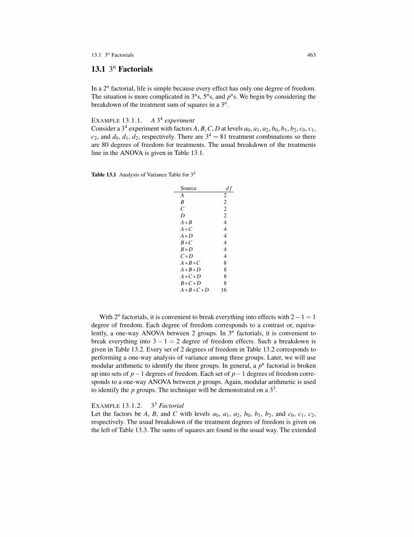
EXAMPLE 13.1.1. A 34 experimentConsider a 34 experiment with factors A, B, C, D at levels a0, a1, a2, b0, b1, b2, c0, c1,c2, and d0, d1, d2, respectively. There are 34 = 81 treatment combinations so thereare 80 degrees of freedom for treatments. The usual breakdown of the treatmentsline in the ANOVA is given in Table 13.1.

Table 13.1 Analysis of Variance Table for 34

Source d fA 2B 2C 2D 2A∗B 4A∗C 4A∗D 4B∗C 4B∗D 4C ∗D 4A∗B∗C 8A∗B∗D 8A∗C ∗D 8B∗C ∗D 8A∗B∗C ∗D 16

With 2n factorials, it is convenient to break everything into effects with 2−1 = 1degree of freedom. Each degree of freedom corresponds to a contrast or, equiva-lently, a one-way ANOVA between 2 groups. In 3n factorials, it is convenient tobreak everything into 3− 1 = 2 degree of freedom effects. Such a breakdown isgiven in Table 13.2. Every set of 2 degrees of freedom in Table 13.2 corresponds toperforming a one-way analysis of variance among three groups. Later, we will usemodular arithmetic to identify the three groups. In general, a pn factorial is brokenup into sets of p−1 degrees of freedom. Each set of p−1 degrees of freedom corre-sponds to a one-way ANOVA between p groups. Again, modular arithmetic is usedto identify the p groups. The technique will be demonstrated on a 33.

EXAMPLE 13.1.2. 33 FactorialLet the factors be A, B, and C with levels a0, a1, a2, b0, b1, b2, and c0, c1, c2,respectively. The usual breakdown of the treatment degrees of freedom is given onthe left of Table 13.3. The sums of squares are found in the usual way. The extended


Table 13.2 Extended Analysis of Variance Table for a 34

Source d f Source d f Source d fA 2 ABC 2 ABCD 2B 2 ABC2 2 ABCD2 2C 2 AB2C 2 ABC2D 2D 2 AB2C2 2 ABC2D2 2AB 2 ABD 2 AB2CD 2AB2 2 ABD2 2 AB2CD2 2AC 2 AB2D 2 AB2C2D 2AC2 2 AB2D2 2 AB2C2D2 2AD 2 ACD 2AD2 2 ACD2 2BC 2 AC2D 2BC2 2 AC2D2 2BD 2 BCD 2BD2 2 BCD2 2CD 2 BC2D 2CD2 2 BC2D2 2

breakdown is given on the right of Table 13.3. It is this breakdown that we willdescribe in detail. Each sum of squares is computed from a one-way analysis ofvariance on three groups. We focus on identifying the appropriate groups.

Table 13.3 Analysis of Variance Table for 33

Source d f Source d fA 2 A 2B 2 B 2C 2 C 2

A∗B 4 AB 2AB2 2

A∗C 4 AC 2AC2 2

B∗C 4 BC 2BC2 2

A∗B∗C 8 ABC 2ABC2 2AB2C 2AB2C2 2

As usual, the sum of squares for A is found by doing a one-way analysis ofvariance on three sample means, the mean of all observations that got treatment a0,the mean of all observations that got treatment a1, and the mean of all observationsthat got treatment a2. There are three treatments so A has 2 degrees of freedom. Themain effects for B and C work similarly.


The standard way of getting the sum of squares for the A∗B interaction involvesdoing a one-way analysis of variance on nine sample means, the means of all obser-vations that got treatments a0b0, a0b1, a0b2, a1b0, a1b1, a1b2, a2b0, a2b1, and a2b2.This has 8 degrees of freedom. From this one-way ANOVA, the sum of squares forA and the sum of squares for B are subtracted, leaving the A ∗B interaction sum ofsquares with 8−2−2 = 4 degrees of freedom.

In the new analysis, the A ∗ B interaction term is broken into two interactionterms, one is called AB while the other is called AB2. The AB term defines a groupof three sample means. These three means have a one-way ANOVA performed onthem yielding 2 degrees of freedom and a sum of squares. Similarly, the AB2 termdefines another group of three sample means for which a one-way is performedyielding 2 degrees of freedom and a sum of squares. By pooling together the degreesof freedom and sums of squares from the new AB and AB2 terms, we can reconstructthe old A∗B term with 4 degrees of freedom.

The analysis of the new AB and AB2 terms is straightforward, just two one-wayANOVAs. The trick is in specifying the observations that go into forming the threesample means. The specification involves the use of modular arithmetic applied tothe subscripts that identify the treatments. Specifically, in a 3n factorial, the arith-metic is performed mod 3. In other words, arithmetic is performed in the usual wayto get a number but the final answer is reported as the remainder when this number isdivided by 3. For the AB interaction, the a and b subscripts are added together. Afteradjusting the numbers mod 3, we have three groups based on the sum of the sub-scripts. In other words, if we let x1, x2, and x3 denote the subscripts of a treatment,the process involves finding (1)x1 +(1)x2 +(0)x3 mod 3; the result is always either0, 1 or 2. The three groups are determined by this value. The 0 group consists of alltreatments that yield a 0. The 1 group has all treatments that yield a 1. The 2 grouphas all treatments that yield a 2. The process is illustrated in Table 13.4. The groupsare also reported in Table 13.5. Without replication, each treatment yields one yvalue. The 9 y values for group 0 are averaged to find a sample mean for group 0.Similarly, sample means are computed for groups 1 and 2. The mean square for AB,say MS(AB), is the sample variance of the three means times 9, the number of ob-servations in each mean. The mean squared multiplied by (3−1) gives SS(AB), thesum of squares for AB.


Table 13.4 AB Interaction Groups

subscripts AB = A1B1C0 Grouptreatment (x1,x2,x3) (1)x1 +(1)x2 +(0)x3 (mod 3)

a0b0c0 (0,0,0) 0 0a0b0c1 (0,0,1) 0 0a0b0c2 (0,0,2) 0 0a0b1c0 (0,1,0) 1 1a0b1c1 (0,1,1) 1 1a0b1c2 (0,1,2) 1 1a0b2c0 (0,2,0) 2 2a0b2c1 (0,2,1) 2 2a0b2c2 (0,2,2) 2 2a1b0c0 (1,0,0) 1 1a1b0c1 (1,0,1) 1 1a1b0c2 (1,0,2) 1 1a1b1c0 (1,1,0) 2 2a1b1c1 (1,1,1) 2 2a1b1c2 (1,1,2) 2 2a1b2c0 (1,2,0) 3 0a1b2c1 (1,2,1) 3 0a1b2c2 (1,2,2) 3 0a2b0c0 (2,0,0) 2 2a2b0c1 (2,0,1) 2 2a2b0c2 (2,0,2) 2 2a2b1c0 (2,1,0) 3 0a2b1c1 (2,1,1) 3 0a2b1c2 (2,1,2) 3 0a2b2c0 (2,2,0) 4 1a2b2c1 (2,2,1) 4 1a2b2c2 (2,2,2) 4 1

Table 13.5 AB Groups

(1)x1 +(1)x2 +(0)x3 mod 3 Groups0 1 2

a0b0c0 a0b1c0 a0b2c0a0b0c1 a0b1c1 a0b2c1a0b0c2 a0b1c2 a0b2c2a1b2c0 a1b0c0 a1b1c0a1b2c1 a1b0c1 a1b1c1a1b2c2 a1b0c2 a1b1c2a2b1c0 a2b2c0 a2b0c0a2b1c1 a2b2c1 a2b0c1a2b1c2 a2b2c2 a2b0c2


The AB2 groups are found by adding the a subscript to twice the b subscript.Computation of the groups for AB2 is illustrated in Table 13.6. The groups are alsogiven in Table 13.7. The computations for MS(AB2) and SS(AB2) are similar to thecomputations for MS(AB) and SS(AB). Recall that SS(AB) and SS(AB2), each with2 degrees of freedom, can be added to get SS(A∗B).

Confounding and fractional replication are based on the 2 degree of freedom ef-fects. The analysis of data from experiments designed using these concepts requiresthe ability to compute the sums of squares for certain 2 degree of freedom effects.

Table 13.6 AB2 Interaction Groups

subscripts AB2 = A1B2C0 Grouptreatment (x1,x2,x3) (1)x1 +(2)x2 +(0)x3 (mod 3)

a0b0c0 (0,0,0) 0 0a0b0c1 (0,0,1) 0 0a0b0c2 (0,0,2) 0 0a0b1c0 (0,1,0) 2 2a0b1c1 (0,1,1) 2 2a0b1c2 (0,1,2) 2 2a0b2c0 (0,2,0) 4 1a0b2c1 (0,2,1) 4 1a0b2c2 (0,2,2) 4 1a1b0c0 (1,0,0) 1 1a1b0c1 (1,0,1) 1 1a1b0c2 (1,0,2) 1 1a1b1c0 (1,1,0) 3 0a1b1c1 (1,1,1) 3 0a1b1c2 (1,1,2) 3 0a1b2c0 (1,2,0) 5 2a1b2c1 (1,2,1) 5 2a1b2c2 (1,2,2) 5 2a2b0c0 (2,0,0) 2 2a2b0c1 (2,0,1) 2 2a2b0c2 (2,0,2) 2 2a2b1c0 (2,1,0) 4 1a2b1c1 (2,1,1) 4 1a2b1c2 (2,1,2) 4 1a2b2c0 (2,2,0) 6 0a2b2c1 (2,2,1) 6 0a2b2c2 (2,2,2) 6 0

Each effect determines the coefficients of the formula to be evaluated. The for-mula is then applied to the subscripts identifying each treatment to identify treatmentgroups. In general, the exponents of the effect determine the formula. The effect ABhas AB = A1B1C0 so the formula is (1)x1 +(1)x2 +(0)x3 mod 3. The effect AB2

has AB2 = A1B2C0 so the formula is (1)x1 +(2)x2 +(0)x3 mod 3. The effect B hasB = A0B1C0 and thus the formula is (0)x1 +(1)x2 +(0)x3 mod 3. The effect AB2Chas AB2C = A1B2C1 and formula (1)x1 +(2)x2 +(1)x3 mod 3. All of the groups for


Table 13.7 AB2 Groups

(1)x1 +(2)x2 +(0)x3 mod 3 Groups0 1 2


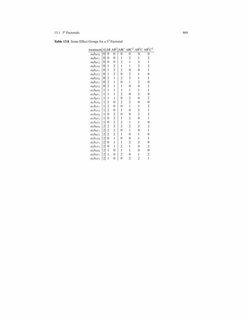
the effects A, AB, AB2, ABC, ABC2, AB2C, and AB2C2 are given in Table 13.8. No-tice that the effects always have a first superscript of 1, e.g., AB2C but never A2B2C.This has to do with redundancy in the formulas and will be discussed further in thesubsection on Fractional Replication.


Table 13.8 Some Effect Groups for a 33 Factorial

treatment A AB AB2 ABC ABC2 AB2C AB2C2

a0b0c0 0 0 0 0 0 0 0a0b0c1 0 0 0 1 2 1 2a0b0c2 0 0 0 2 1 2 1a0b1c0 0 1 2 1 1 2 2a0b1c1 0 1 2 2 0 0 1a0b1c2 0 1 2 0 2 1 0a0b2c0 0 2 1 2 2 1 1a0b2c1 0 2 1 0 1 2 0a0b2c2 0 2 1 1 0 0 2a1b0c0 1 1 1 1 1 1 1a1b0c1 1 1 1 2 0 2 0a1b0c2 1 1 1 0 2 0 2a1b1c0 1 2 0 2 2 0 0a1b1c1 1 2 0 0 1 1 2a1b1c2 1 2 0 1 0 2 1a1b2c0 1 0 2 0 0 2 2a1b2c1 1 0 2 1 2 0 1a1b2c2 1 0 2 2 1 1 0a2b0c0 2 2 2 2 2 2 2a2b0c1 2 2 2 0 1 0 1a2b0c2 2 2 2 1 0 1 0a2b1c0 2 0 1 0 0 1 1a2b1c1 2 0 1 1 2 2 0a2b1c2 2 0 1 2 1 0 2a2b2c0 2 1 0 1 1 0 0a2b2c1 2 1 0 2 0 1 2a2b2c2 2 1 0 0 2 2 1


13.2 Column Space Considerations

Consider a 32 factorial. The ANOVA table can be broken up in two ways. The usualmethod with 4 degrees of freedom for interaction and the new method in which theinteraction is divided into two 2 degree of freedom parts.

Source d f Source d fA 2 A 2B 2 B 2

A∗B 4 AB 2AB2 2

Table 13.9 gives the treatment groups that are determined by the AB and AB2 inter-action groups. The groups from Table 13.9 have been rearranged into the form

B0 1 2

0 AB(0)AB2(0) AB(1)AB2(2) AB(2)AB2(1)A 1 AB(1)AB2(1) AB(2)AB2(0) AB(0)AB2(2)

2 AB(2)AB2(2) AB(0)AB2(1) AB(1)AB2(0)

Note that this arrangement is really a Graeco-Latin square. Each of AB(0), AB(1),and AB(2) appears in every row and in every column, the same is true for AB2(0),AB2(1), and AB2(2), moreover each of AB(0), AB(1), and AB(2) appears exactlyonce with every AB2 group.

Table 13.9 AB and AB2 Interaction Groups

subscripts AB = A1B1 Group AB2 = A1B2 Grouptreatment (x1,x2) (1)x1 +(1)x2 (mod 3) (1)x1 +(2)x2 (mod 3)

a0b0 (0,0) 0 0 0 0a0b1 (0,1) 1 1 2 2a0b2 (0,2) 2 2 4 1a1b0 (1,0) 1 1 1 1a1b1 (1,1) 2 2 3 0a1b2 (1,2) 3 0 5 2a2b0 (2,0) 2 2 2 2a2b1 (2,1) 3 0 4 1a2b2 (2,2) 4 1 6 0

The usual linear model for a 3×3 factorial with interaction but no replication is

13.2 Column Space Considerations 471

y00y01y02y10y11y12y20y21y22

= X

µα0α1α2β0β1β2

(α ∗β )00(α ∗β )01(α ∗β )02(α ∗β )10(α ∗β )11(α ∗β )12(α ∗β )20(α ∗β )21(α ∗β )22

+ e

where

X =

1 1 0 0 1 0 0 1 0 0 0 0 0 0 0 01 1 0 0 0 1 0 0 1 0 0 0 0 0 0 01 1 0 0 0 0 1 0 0 1 0 0 0 0 0 01 0 1 0 1 0 0 0 0 0 1 0 0 0 0 01 0 1 0 0 1 0 0 0 0 0 1 0 0 0 01 0 1 0 0 0 1 0 0 0 0 0 1 0 0 01 0 0 1 1 0 0 0 0 0 0 0 0 1 0 01 0 0 1 0 1 0 0 0 0 0 0 0 0 1 01 0 0 1 0 0 1 0 0 0 0 0 0 0 0 1

.

Building a model based on a grand mean and effects for each of the A, B, AB,and AB2 groupings gives

y00y01y02y10y11y12y20y21y22

=

1 1 0 0 1 0 0 1 0 0 1 0 01 1 0 0 0 1 0 0 1 0 0 0 11 1 0 0 0 0 1 0 0 1 0 1 01 0 1 0 1 0 0 0 1 0 0 1 01 0 1 0 0 1 0 0 0 1 1 0 01 0 1 0 0 0 1 1 0 0 0 0 11 0 0 1 1 0 0 0 0 1 0 0 11 0 0 1 0 1 0 1 0 0 0 1 01 0 0 1 0 0 1 0 1 0 1 0 0

µα0α1α2β0β1β2

(αβ )0(αβ )1(αβ )2(αβ 2)0(αβ 2)1(αβ 2)2

+ e


Note that the column space of the design matrix is the same in each model, i.e.,R9. Since the columns corresponding to µ , the αs, and the β s are the same in eachmodel, the interaction space — which is the space orthogonal to that spanned by µ ,the αs, and β s — must be the same for each model. However, after adjusting for thegrand mean, i.e. using Gram-Schmidt to orthogonalize with respect to the column of1s, the columns corresponding to the (αβ ) terms are orthogonal to the columns forthe α terms, the β terms, and also the (αβ 2) terms. Similarly, the columns for the(αβ 2) terms are orthogonal to all of the other sets of columns. To see this, observethat after adjusting everything for a column of 1s, the X matrix becomes

1 2 −1 −1 2 −1 −1 2 −1 −1 2 −1 −11 2 −1 −1 −1 2 −1 −1 2 −1 −1 −1 21 2 −1 −1 −1 −1 2 −1 −1 2 −1 2 −11 −1 2 −1 2 −1 −1 −1 2 −1 −1 2 −11 −1 2 −1 −1 2 −1 −1 −1 2 2 −1 −11 −1 2 −1 −1 −1 2 2 −1 −1 −1 −1 21 −1 −1 2 2 −1 −1 −1 −1 2 −1 −1 21 −1 −1 2 −1 2 −1 2 −1 −1 −1 2 −11 −1 −1 2 −1 −1 2 −1 2 −1 2 −1 −1

.

The last three columns corresponding to the (αβ 2) terms are orthogonal to every-thing else, and columns 8, 9, 10 corresponding to the (αβ ) terms are orthogonal toeverything else. Each of these sets of 3 columns must be in the interaction space be-cause they are orthogonal to the columns for µ , the αs, and β s. Since they are alsoorthogonal to each other, they are breaking the interaction into 2 orthogonal pieces.Finally, the interaction columns were originally just group indicators, so the sumsof squares for the one-way ANOVA on these groups will give the sum of squaresappropriate for these sets of orthogonal columns.

13.3 Confounding and Fractional Replication

Having identified the groups associated with each 2 degree of freedom effect, wecan now consider the issues of confounding and fractional replication. Confoundingis a process for determining incomplete blocks, i.e., blocks that do not contain allof the treatments, but confounding retains a relatively simple analysis for the data.Fractional replication is a process for constructing experiments that do not containall of the factorial treatments but retains an analysis of the data that allows one toidentify important effects.

13.3 Confounding and Fractional Replication 473

13.3.1 Confounding

We begin with a discussion of confounding. We can pick an effect, say, ABC todefine blocks of size 9 in a 33 experiment. The effect ABC divides the treatmentsinto three groups, the three groups define three blocks of 9 treatments. The groupsare identified in Table 13.8 and the blocks are given in Table 13.10. Alternatively, wecould use AB2C2 to define three different blocks of 9. These are given in Table 13.11.

Table 13.10 ABC Defining Three Blocks of Nine

Block Block Block0 1 2


With ABC defining blocks, two degrees of freedom are confounded with the threeblocks but the other 6 degrees of freedom involving A∗B∗C interactions are avail-able in ABC2, AB2C, and AB2C2. It is at this point, and not before, that the analysisrequires computation of sums of squares for individual 2 degree of freedom interac-tion effects.

Table 13.11 AB2C2 Defining Three Blocks of Nine

Block Block BlockAB2C2(0) AB2C2(1) AB2C2(2)


We can also use two effects to create 9 blocks of size three. If we use ABC andAB2C2 to define blocks, one group consists of the three treatments in the ABC(0)group that are also in the AB2C2(0) group. Another group of three has both ABC(0)


and AB2C2(1). The 9 blocks of three run through ABC(i) and AB2C2( j) for i, j =0,1,2. Table 13.12 gives the 9 blocks defined by ABC and AB2C2.

Table 13.12 ABC, AB2C2 Defining Nine Blocks of Three

ABC(0) ABC(1) ABC(2)a0b0c0 a2b0c2 a1b0c1

AB2C2(0) a0b1c2 a2b1c1 a1b1c0a0b2c1 a2b2c0 a1b2c2a2b0c1 a1b0c0 a0b0c2

AB2C2(1) a2b1c0 a1b1c2 a0b1c1a2b2c2 a1b2c1 a0b2c0a1b0c2 a0b0c1 a2b0c0

AB2C2(2) a1b1c1 a0b1c0 a2b1c2a1b2c0 a0b2c2 a2b2c1

As in 2n factorials, when more than one effect is used to define groups (blocks),other effects also determine the same groups (are confounded with blocks). With9 blocks, there are 8 degrees of freedom for blocks. The defining effects, ABC andAB2C2, are confounded with blocks but these account for only 4 degrees of freedom.There are 4 additional degrees of freedom for blocks and since each effect has 2degrees of freedom, two additional effects are implicitly confounded with blocks.Again as in 2n factorials, the implicitly confounded effects can be identified usingmodular multiplication, however, the multiplication works differently. Exponentsare now evaluated modulo 3. Multiplying the two defining effects gives

ABC×AB2C2 = A2B3C3 = A2.

We never allow the first superscript in an effect to be 2. To eliminate such terms ina 3n experiment, raise the term to the 3−1 power,

A2 = (A2)2 = A4 = A.

(More on this issue of the first superscript later.) Thus when confounding both ABCand AB2C2, the main effect A is also confounded. We can see this directly fromTable 13.12, where the level of A is constant in every block, i.e., the a subscript isthe same in every block. One more effect is implicitly confounded with blocks; itcan be identified by multiplying one defining effect times the square of the othereffect, i.e.,

ABC× (AB2C2)2 = A3B5C5 = B2C2 = (B2C2)2 = B4C4 = BC.

It is irrelevant which effect is squared, the result is the same either way.Performing a 3n experiment in 27 blocks of size 3n−3 requires the use of three

defining effects. These are effects such as ABCD, ABC2D, and AB2CD2, but we willrefer to them generically as α , β , and γ . With 27 blocks there are 26 degrees of


freedom for blocks. Each effect has 2 degrees of freedom, so there are 13 effectsconfounded with blocks. Three of the effects are the defining effects α , β , and γ .The other ten effects can be obtained through multiplying pairs of factors,

α(β ), α(β )2, α(γ), α(γ)2, β (γ), β (γ)2

and multiplying all three factors,

αβγ , αβγ2, αβ 2γ, αβ 2γ2.

Just to illustrate the method of finding the effects that are confounded, sup-pose AB, CD and EF are the defining effects. The effects that are implicitly con-founded are ABCD, AB(CD)2, ABEF , AB(EF)2, CDEF , CD(EF)2, ABCDEF ,ABCD(EF)2, AB(CD)2EF , AB(CDEF)2.

13.3.2 Fractional Replication

Any one of the three blocks in Table 13.10 defines a 1/3 rep. of the 33 factorialbased on ABC. Similarly, any one of the three blocks in Table 13.11 defines a 1/3rep. of the 33 factorial based on AB2C2.

In fractional replication, many effects will be lost. In a 1/2 rep. of a 2n factorial,about 1/2 of the effects are lost to aliasing. In a 1/3 rep. of a 3n factorial, about2/3s of the effects are lost to aliasing. It is vital to identify the aliasing structurein fractional replications. To do this, we need to delve a bit deeper into modulararithmetic.

Recall that the first term in all of our effects always has a power of 1, e.g., AB2C2

but never A2B2C2, also BC2 but never B2C. The first term always has a power of 1because having any larger power is redundant. The groups defined by an effect, say,AB2C2 are determined by the value of

z = [(1)x1 +(2)x2 +(2)x3] mod 3

where (x1,x2,x3) are the subscripts of the treatments (a,b,c). If we double the co-efficients in the equation we get

z = [(2)x1 +(4)x2 +(4)x3] mod 3= [(2)x1 +(1)x2 +(1)x3] mod 3.

Here we have also adjusted the coefficients using modular arithmetic. For example,it is easy to see that with an integer x, 4x mod 3 = x mod 3. The groups defined bythis second equation correspond to

A2B4C4 = A2B1C1 = A2BC,


where we are again using modular multiplication. The point is that the two setsof equations for AB2C2 and A2BC give identical groups. Every treatment that is ingroup 0 for AB2C2 is also in group 0 for A2BC. Every treatment that is in group 1for AB2C2 is in group 2 for A2BC and every treatment that is in group 2 for AB2C2

is in group 1 for A2BC. Thus,

AB2C2 ≡ A2BC.

Generally, if we take any power of an effect where the power is a positive integerless than p = 3, we still have the same effect because the new modular equationgives the same groups. To have a unique way of writing each effect, we never allowthe first superscript in an effect to be greater than 1. When given an effect with alead term having an exponent of 2, squaring the term reduces the exponent withoutchanging the effect, e.g.,

A2BC =(A2BC

)2= A4B2C2 = AB2C2.

Modular multiplication and the equivalences between effects are crucial to iden-tifying aliases. In a 1/3 rep. based on ABC, the aliases of an effect are determinedfrom multiplying the effect by ABC and (ABC)2. For example, the main effect A isaliased with two other effects

A×ABC = A2BC =(A2BC

)2= A4B2C2 = AB2C2

andA× (ABC)2 = A3B2C2 = B2C2 =

(B2C2)2

= B4C4 = BC.

The interaction effect BC2 is aliased with two effects

BC2 ×ABC = AB2C3 = AB2

andBC2 × (ABC)2 = A2B3C4 = A2C =

(A2C

)2= A4C2 = AC2.

Tables 13.13 and 13.14 give all the multiplications for determining the aliasingstructure for the 1/3 rep. based on ABC. The aliasing structure of this examplecan be determined from either Table 13.13 or 13.14 by simply listing all of theequalities. The aliasing structure reduces to

A = AB2C2 = BC,

B = AB2C = AC,

C = ABC2 = AB,

andAB2 = AC2 = BC2

with the defining effect ABC lost (confounded with the grand mean).


Table 13.13 First Aliasing Table for a 1/3 Rep. of a 33 Based on ABC

Source ×ABCA = A2BC = AB2C2

B = AB2C = AB2CC = ABC2 = ABC2

AB = A2B2C = ABC2

AB2 = A2B3C = AC2

AC = A2BC2 = AB2CAC2 = A2BC3 = AB2

BC = AB2C2 = AB2C2

BC2 = AB2C3 = AB2

ABC = A2B2C2 = ABC*ABC2 = A2B2C3 = ABAB2C = A2B3C2 = ACAB2C2 = A2B3C3 = A

Table 13.14 Second Aliasing Table for a 1/3 Rep. of a 33 Based on ABC

Source ×A2B2C2

A = A3B2C2 = BCB = A2B3C2 = ACC = A2B2C3 = ABAB = A3B3C2 = CAB2 = A3B4C2 = BC2

AC = A3B2C3 = BAC2 = A3B2C4 = BC2

BC = A2B3C3 = ABC2 = A2B3C4 = AC2

ABC = A3B3C3 = —ABC2 = A3B3C4 = CAB2C = A3B4C3 = BAB2C2 = A3B4C4 = BC

A 1/9 rep. of a 33 can be obtained by using just one of the 9 blocks given inTable 13.12. Typically one would not perform a 1/9th rep. of something as small asa 33, but we will discuss the issues involved to illustrate the principles. They extendeasily to general 3n systems. Table 13.12 uses the defining effects ABC and AB2C2.As with 2n systems, there are additional effects lost when more than one definingeffect is used. The effects

ABC×AB2C2 = A2B3C3 = A2 = A

andABC×

(AB2C2)2

= A3B5C5 = B2C2 = BC.


are also (implicitly) defining effects. Note that squaring both terms in the multipli-cations just leads to redundancies, e.g.,

(ABC)2 ×AB2C2 = BC.

To find the aliases for an effect, say B, we need to multiply the effect by all fourof the defining effects and by the squares of all the defining effects. Thus B has thefollowing aliases,

B×ABC = AB2C

B× (ABC)2 = AC

B×AB2C2 = AC2

B×(AB2C2)2

= ABC2

B×A = AB

B×A2 = AB2

B×BC = BC2

B×B2C2 = C

orB =C = AB = AB2 = AC = AC2 = BC2 = ABC2 = AB2C.

In this example, all of the effects that are not used in defining the 1/9th rep. arealiased with each other. In a 1/9th rep. of a 33, only three treatments are used sothere are only 2 degrees of freedom for treatments. Every effect has two degrees offreedom so there is only one effect available; it can be called anything except one ofthe effects that define the fractional rep.

EXAMPLE 13.3.3. A 35 FactorialWith only 27 treatments in a 33, it would not be of much value to consider a 1/9threp. However a 35 has 243 treatments, so a 1/9th rep. reduces the problem to a moremanageable 27 treatments. With factors A, B, C, D, E, we might use ABC2D andBC2DE2 as defining effects. The groups are defined using the ABC2D equation

z1 = [x1 + x2 +2x3 + x4 +0x5] mod 3

and the BC2DE2 equation

z2 = [0x1 + x2 +2x3 + x4 +2x5] mod 3

where (x1,x2,x3,x4,x5) denotes the subscripts of a treatment combination and thecoefficients in the equations are determined by the superscripts in the defining ef-fects. The treatments that have, say, z1 = 1 are referred to as the ABC2D(1) groupwith similar definitions for z1 = 0,2 and groups ABC2D(0) and ABC2D(2). BC2DE2

groups are denoted in the same way based on the values of z2. Thus a0b0c0d0e0 is inthe group defined by ABC2D(0) and BC2DE2(0), while a0b1c2d1e1 is in the group

13.4 Analysis of a Confounded 33 479

defined by ABC2D(0) and BC2DE2(2), and a1b1c1d1e1 is in the group defined byABC2D(2) and BC2DE2(0).

The two defining effects ABC2D and BC2DE2 determine 9 blocks of 27 treat-ments. Any one of the blocks can be used as a 1/9 rep. In a 1/9 rep., other effectsare implicit defining effects, namely

BC2DE2 ×ABC2D = AB2C2D2E

andBC2DE2 ×

(ABC2D

)2= A2B3C6D3E2 = A2E2 = AE.

An effect, say B, has the following aliases,

B×ABC2D = AB2C2D

B×(ABC2D

)2= AC2D

B×BC2DE2 = BCD2E

B×(BC2DE2)2

= CD2E

B×AB2C2D2E = AC2D2E

B×(AB2C2D2E

)2= ABC2D2E

B×AE = ABE

B×A2E2 = AB2E

or

B = ABE = AB2E = AC2D =CD2E =

AB2C2D = AC2D2E = BCD2E = ABC2D2E.

13.4 Analysis of a Confounded 33

The data in Table 13.15 are adapted from Kempthorne (1952). The experiment con-cerns the effects of three factors on the sugar content in sugar beets. The dependentvariable is (%sugar− 16)100. The three factors are D – the sowing date, S – thespacings of the rows, and N – the amount of fertilizer (sulphate of ammonia) ap-plied. In Table 13.15 the treatments are identified by their subscripts alone. Theexperiment was performed in 2 replications. Each replication has 9 blocks of size3. In the first replication DS2N and SN are confounded with blocks. In the secondreplication DS2N2 and DN are confounded. Thus we introduce partial confoundingfor 3ns in this analysis.

The defining effects for the blocks in Rep. 1 are DS2N and SN. It follows that

DS2N ×SN = DN2


andDS2N × (SN)2 = DS

are also confounded with blocks in Rep. 1. Similarly, the defining effects for theblocks in Rep. 2 are DS2N2 and DN, so DS and SN2 are also confounded withblocks in Rep. 2. Note that DS is confounded with blocks in both replications, sothere is no information available on DS.

Table 13.15 Sugar Beet Data

Rep. 1 Rep. 2dsn y dsn y dsn y dsn y dsn y dsn y000 79 110 62 102 79 000 47 202 42 012 10121 44 022 −2 011 105 211 43 021 36 220 108212 59 201 53 220 56 122 30 110 44 101 33100 85 001 100 111 105 112 39 100 88 121 79221 36 210 105 020 50 020 21 011 53 002 18012 70 122 79 202 50 201 39 222 39 210 88200 59 222 21 211 96 102 44 212 42 200 27112 13 101 47 120 65 010 33 120 105 111 4021 70 010 30 002 85 221 68 001 27 022 56In Rep. 1 the defining effects for blocks are DS2N and SNwith DN2 and DS also confounded. In Rep. 2 the defining effects for blocksare DS2N2 and DN with SN2 and DS also confounded.

One version of the analysis of variance table is given as Table 13.16. In thisversion the interactions are not broken into 2 degree of freedom effects. Minitab’s“glm” command will give this analysis of variance table. The necessary commandsare given below.

MTB > names c2 ’D’ c3 ’S’ c4 ’N’ c5 ’y’ c6 ’Blks’MTB > glm c5 = c6 c2|c3|c4

The model involves Blocks and a full factorial analysis on the three factors. Theblocks are just listed from 1 to 18. To get the correct analysis, the blocks must belisted in the glm command before the treatment factors. The output from the glmcommand provides two sets of degrees of freedom: model degrees of freedom, i.e.,what one would normally expect to have for degrees of freedom, and reduced de-grees of freedom. The reduced degrees of freedom are appropriate. When the modeland reduced degrees of freedom differ, the reduced number has a + after it to em-phasize the difference. For example, under normal conditions the D ∗ S interactionwould have 4 degrees of freedom, however D ∗ S has been decomposed into DS,which is completely confounded with blocks, and DS2. The 2 degrees of freedom inthe table for D∗S are just the two degrees of freedom for DS2.

The most remarkable thing about Table 13.16 is the fact that the F statistics are souniformly small. If I were getting paid to analyze these data I would have a serioustalk with the people who conducted the experiment to see whether some explanation


Table 13.16 Analysis of Variance for Confounded Sugar Beet Experiment

Source d f SS MS FBlks 17 17416.00 1024.47 0.81D 2 838.78 419.39 0.34S 2 60.78 30.39 0.02N 2 4177.33 2088.67 1.65D∗S 2 238.78 119.39 0.09D∗N 4 1692.22 423.06 0.33S∗N 4 898.89 224.72 0.18D∗S∗N 8 2724.22 340.53 0.27Error 12 15178.33 1264.86Total 53 43225.33

of this could be found. In the present context, our primary concern is not the databut the process of analyzing the data.

13.4.1 The Expanded ANOVA Table

We now consider the expanded ANOVA table in which the interactions are brokeninto 2 degree of freedom effects. The expanded table is presented as Table 13.17.In Table 13.17, the first line of Table 13.16 has been broken into Reps and Blockswithin Reps. The mean square for Blocks in Table 13.16 is computed from the 18block means. Each block mean is the average of 3 observations. The mean square forReps in Table 13.17 is computed from the two replication means. Each Rep. meanis averaged over 27 observations. To compute the sum of squares for Blocks withinReps, subtract the sum of squares for Reps from the sum of squares for Blocksin Table 13.16. The lines for D, S, and N are identical in the two ANOVA tables;they are computed in the usual way. The three means for any main effect are eachaverages over 18 observations.

The analysis begins to get more complicated when we consider the interactions.The effects DN2, SN, and DS2N are confounded in Rep. 1 but not in Rep. 2, so wecan obtain mean squares and sums of squares for these effects from Rep. 2. Eachof these effects defines three groups of treatments. The sugar content observationsfrom Rep. 2 are listed below for each group along with their means. The means areaverages over 9 observations.


Table 13.17 Analysis of Variance for Confounded Sugar Beet Experiment

Source d f SS MS FReps 1 3552.67 3552.67 2.81Blks(Reps) 16 13863.33 866.46 0.69D 2 838.78 419.39 0.34S 2 60.78 30.39 0.02N 2 4177.33 2088.66 1.65DS2 2 238.78 119.39 0.09DN/Rep 1 2 578.67 289.33 0.23DN2/Rep 2 2 1113.56 556.78 0.44SN/Rep 2 2 170.89 85.44 0.07SN2/Rep 1 2 728.00 364.00 0.29DSN 2 552.33 276.17 0.22DSN2 2 446.33 223.17 0.18DS2N/Rep 2 2 1381.56 690.78 0.55DS2N2/Rep 1 2 344.00 172.00 0.14Error 12 15178.33 1264.86Total 53 43225.33

Groups and Means from Rep. 2DN2 SN DS2N

0 1 2 0 1 2 0 1 247 43 30 47 30 43 47 30 4342 44 36 36 44 42 44 42 3633 10 108 10 33 108 108 10 3321 39 39 39 39 21 39 21 3939 88 53 88 39 53 53 88 3979 18 88 79 88 18 79 88 1833 68 44 68 33 44 44 68 3342 105 27 42 27 105 42 27 1054 56 27 27 56 4 56 4 27

37.7̄ 52.3̄ 50.2̄ 48.4̄ 43.2̄ 48.6̄ 56.8̄ 42.0 41.4̄

The mean square for DN2 is 9 times the sample variance of 37.7̄, 52.3̄, and 50.2̄.The mean squares for SN and DS2N are found similarly.

The effects DS2N2, DN, and SN2 are confounded in Rep. 2 but not in Rep. 1so we can obtain mean squares and sums of squares for these effects from Rep.1. Again, each of the effects defines three groups of treatments. The sugar contentobservations from Rep. 1 are listed below for each group along with their means.The means are again averages over 9 observations and the mean square for eacheffect is 9 times the sample variance of the three group means.


Groups and Means from Rep. 1DN SN2 DS2N2

0 1 2 0 1 2 0 1 279 59 44 79 59 44 79 44 5953 62 −2 −2 53 62 62 53 −279 105 56 105 56 79 56 105 7936 85 70 85 70 36 70 85 3679 100 105 79 100 105 79 105 10050 50 105 105 50 50 50 50 10513 70 59 59 13 70 70 13 5930 21 47 21 47 30 47 21 3096 65 85 96 65 85 96 85 65

57.2̄ 68.5̄ 63.2̄ 69.6̄ 57.0 62.3̄ 67.6̄ 62.3̄ 59.0

There are three interaction effects remaining: DS2, DSN, and DSN2. None ofthese effects are confounded in either replication so their mean squares are com-puted from the complete data. The observations in the three groups for DS2 aregiven below with their means.

DS2 Groups and Means from Complete DataDS2(0) DS2(1) DS2(2)

79 12 39 59 70 21 44 59 3962 21 39 −2 47 88 53 30 5356 85 18 79 96 88 105 65 7936 47 68 85 43 44 70 30 33

100 44 27 105 36 42 79 42 105105 108 4 50 33 56 50 10 27

52.83̄ 57.77̄ 54.05̄

The mean square for DS2 is 18 times the sample variance of the three means. Theobservations in the three groups for DSN are given below with their means.

DSN Groups and Means from Complete DataDSN(0) DSN(1) DSN(2)79 70 39 44 13 39 59 59 2153 21 39 −2 30 88 62 47 5379 65 88 56 96 79 105 85 1870 47 44 85 43 33 36 30 68

105 36 105 100 42 27 79 44 42105 10 4 50 108 56 50 33 27

58.83̄ 54.83̄ 51.00

Finally, the observations in the three groups for DSN2 are given below with theirmeans.

DSN2 Groups and Means from Complete DataDSN2(0) DSN2(1) DSN2(2)79 13 39 59 70 39 44 59 21−2 47 53 53 30 88 62 21 39105 65 88 56 85 18 79 96 7936 47 68 85 30 33 70 43 44

105 42 105 79 36 42 100 44 2750 33 56 105 108 4 50 10 27

57.16̄ 56.66̄ 50.83̄


In general, an effect is estimated from all replications in which it is not confounded.

13.4.2 Interaction Contrasts

Typically, when an interaction effect is of even marginal significance, we investi-gate it further by looking at interaction contrasts. Christensen (1996a, Sec. 7.2.1)and Christensen (1996b, Chapters 11, 12) discuss interaction contrasts in detail. Todefine a contrast in, say, the D ∗N interaction we typically choose a contrast in Dand a contrast in N and combine them to form an interaction contrast. For example,if we use the main effect contrasts 2n0−n1−n2 and d0−d1, the interaction contrastcoefficients are

Nn0 n1 n2

D contrasts 2 −1 −1d0 1 2 −1 −1d1 −1 −2 1 1d2 0 0 0 0

More generally there are 9 contrast coefficients in the body of this table correspond-ing to the 9 D ∗ N combinations d0n0,d0n1, . . . ,d2n2. The actual coefficients areobtained by multiplying the D contrast coefficients by the N contrast coefficients. Ingeneral, an interaction contrast is defined by contrast coefficients

ND n0 n1 n2d0 q00 q01 q02d1 q10 q11 q12d2 q20 q21 q22

where the sum of the qi js over each row and over each column equals 0. We nowexamine how this approach to interaction contrasts relates to the analysis just givenfor a confounded 3n.

Consider again the D ∗N interaction. It has been decomposed into two parts,DN and DN2. At one level, it is very easy to find interaction contrasts in DN andDN2. For example, DN defines three groups DN(0), DN(1), and DN(2) with samplemeans from Rep. 1 of 57.2̄, 68.5̄, and 63.2̄, respectively. To obtain the DN sumof squares, we simply performed a one-way ANOVA on the three group means.Continuing our analogy with one-way ANOVA, DN has two degrees of freedom sowe can find two orthogonal contrasts in DN. In particular, we can define orthogonalcontrasts in the DN groups, say

DN1 ≡ (3)[DN(0)]+(−3)[DN(1)]+(0)[DN(2)], (1)

which compares 3 times the DN(0) group mean with 3 times the DN(1) group mean,and


DN2 ≡ (3)[DN(0)]+(3)[DN(1)]+(−6)[DN(2)],

which is equivalent to comparing the average of groups DN(0) and DN(1) with theDN(2) group mean. The reason for including the factors of 3 in the contrasts willbecome clear later. Estimates and sums of squares for these contrasts are computedin the usual way based on the sample means for the three groups. The computationswill be illustrated later.

We can also define orthogonal contrasts in DN2, say

DN21 ≡ (3)[DN2(0)]+(−3)[DN2(1)]+(0)[DN2(2)]

andDN2

2 ≡ (3)[DN2(0)]+(3)[DN2(1)]+(−6)[DN2(2)].

The appropriate means for estimating the DN2 contrasts are obtained from Rep. 2.At issue is the correspondence between these contrasts in DN and DN2 and con-

trasts in the four degree of freedom interaction D∗N that we usually consider. Thekey to the correspondence is in identifying the treatment groups for DN and DN2

relative to the 9 combinations of a level of D with a level of N. These correspon-dences are given below.

DN Groups DN2 GroupsN N

D n0 n1 n2 D n0 n1 n2d0 0 1 2 d0 0 2 1d1 1 2 0 d1 1 0 2d2 2 0 1 d2 2 1 0

For example, any treatment with d1n2 corresponds to DN group [1+ 2] mod 3 = 0and DN2 group [1+(2)2] mod 3 = 2.

The contrast DN1 in equation (1) compares 3 times group DN(0) to 3 timesDN(1), we can rewrite the contrast as

DN1 ContrastN

D n0 n1 n2d0 1 −1 0d1 −1 0 1d2 0 1 −1

Here the three treatments in group DN(0) have been assigned 1s, the three treat-ments in group DN(1) have been assigned −1s, and the three treatments in groupDN(2) have been assigned 0s. This contrast compares the sum of the 3 treatmentsin the DN(0) group with the sum of the 3 treatments in the DN(1) group. We willcall this the D∗N version of the DN1 contrast. Note that the contrast given is indeedan interaction contrast in D ∗N, because the contrast coefficients in each row andcolumn sum to 0.

The D ∗N version of DN2 can be constructed similarly by assigning 1s to thetreatments in DN(0) and DN(1) and −2s to the treatments in DN(2).


DN2 ContrastN

D n0 n1 n2d0 1 1 −2d1 1 −2 1d2 −2 1 1

The DN2 contrasts, DN21 and DN2

2 can also be written in their D∗N versions.

DN21 Contrast DN2

2 ContrastN N

D n0 n1 n2 D n0 n1 n2d0 1 0 −1 d0 1 −2 1d1 −1 1 0 d1 1 1 −2d2 0 −1 1 d2 −2 1 1

It is a simple matter to check that these four contrasts in the D∗N interaction areorthogonal. Incidentally, this confirms that the DN and DN2 effects are orthogonal.Orthogonality of all the 2 degree of freedom effects was assumed throughout ouranalysis.

Just as the DN contrasts can be written in two ways, we can also obtain theestimates in two ways. Using the group means obtained from Rep. 1, the estimateof DN1 ≡ (3)[DN(0)]+(−3)[DN(1)]+(0)[DN(2)] is

D̂N1 ≡ (3)57.2̄+(−3)68.5̄+(0)63.2̄ =−34.

The estimate of DN2 ≡ (3)[DN(0)]+ (3)[DN(1)]+ (−6)[DN(2)] is obtained simi-larly. Estimates of DN2

1 and DN22 use the group means obtained from Rep. 2. The

variance of D̂N1 is

Var(D̂N1) = σ2[32 +(−3)2 +02]/9 = 2σ2

where the 9 in the denominator of the second term is the number of observationsthat the DN group means are averaged over. The standard error for the estimate ofDN1 is

SE(D̂N1) =√

MSE[32 +(−3)2 +02]/9

The sum of squares for DN1 is

−342

[32 +(−3)2 +02]/9= 578.

Similar computations apply to DN2, DN21 , and DN2

2 .Alternatively, we could apply the D∗N version of DN1 to the means table


D−N Means from Rep. 1N = 3 N

D n0 n1 n2d0 53.0 91.6̄ 51.0d1 70.6̄ 65.3̄ 57.0d2 73.3̄ 61.6̄ 43.3̄

The estimated DN1 contrast in D∗N form is

D̂N1 = 53.0−91.6̄−70.6̄+57.0+61.6̄−43.3̄ =−34.

This is exactly the estimate obtained from the other method. The variance of D̂N1 inD∗N form is

Var(D̂N1) = σ2[12 +(−1)2 +(−1)2 +12 +12 +(−1)2]/3 = 2σ2

where the 3 in the denominator of the middle term is the number of observations ineach mean. The sum of squares is

−342

[12 +(−1)2 +(−1)2 +12 +12 +(−1)2]/3= 578

Of course the variance and the sums of squares from the two methods are identical.We can construct other D ∗N interaction contrasts from the D ∗N forms of the

DN and DN2 contrasts. If we add the DN1 and DN21 contrast coefficients we get

ND n0 n1 n2d0 2 −1 −1d1 −2 1 1d2 0 0 0

This is not only a contrast in D ∗N but it even corresponds to our usual way ofconstructing interaction contrasts from main effect contrasts. It combines 2n0−n1−n2 and d0 −d1.

The new contrast is DN1+DN21 , so the estimate of the new contrast is just D̂N1+

D̂N21 . Recall that D̂N1 is estimated from Rep. 1 and D̂N2

1 is estimated from Rep. 2.

Because DN1 and DN21 are orthogonal contrasts, D̂N1 and D̂N2

1 are independent, thevariance of the new estimate is

Var(D̂N1 + D̂N21 ) = Var(D̂N1)+Var(D̂N2

1 ) = 2σ2 +2σ2,

and the standard error is√

4MSE.


13.5 5n Factorials

We now briefly consider n factors each at 5 levels, i.e., 5n’s. In this case, as in all pn

structures with p a prime number, the methods for 3n factorials extend easily.A 5n can be broken down into groups of 5−1 = 4 degrees of freedom. Consider

two factors A and B at 5 levels, say, a0, a1, a2, a3, a4, and b0, b1, b2, b3, b4. Thereare 52 = 25 treatment combinations aib j for i, j = 0,1,2,3,4. The breakdown into 4degree of freedom effects is illustrated in Table 13.18.

Table 13.18 Analysis of Variance for a 52

Source d f Source d fA 4 A 4B 4 B 4A∗B 16 AB 4

AB2 4AB3 4AB4 4

In a simple extension of our discussion for 3n factorials, the groups of treatmentsdetermined by, say, AB4 correspond to the five values of

z = x1 +4x2 mod 5

where x1 and x2 are the subscripts for the treatment combinations. Table 13.19 givesthe groups for all six of the 4 degree of freedom effects. Table 13.20 rewrites thetreatment groups determined by AB4. Table 13.20 provides a scheme for assigningthe 25 treatments to blocks of size five with AB4 confounded.

Any one of the blocks in Table 13.20 provides a 1/5 replicate of the 52 experi-ment based on AB4. An effect such as A is aliased with

A×AB4 = A2B4 = (A2B4)3 = A6B12 = AB2

A× (AB4)2 = A3B8 = (A3B8)2 = A6B16 = AB

A× (AB4)3 = A4B12 = (A4B12)4 = A16B48 = AB3

A× (AB4)4 = A5B16 = B.

The alias group isA = B = AB = AB2 = AB3.

All effects other than AB4 are aliased together. AB4 is lost because it defines the1/5 rep. Of course a 1/5 rep. of a 52 contains only 5 treatments, so it has only 4degrees of freedom for treatment effects. Each effect has 4 degrees of freedom, sothere could not be more than one treatment effect available in the 1/5 rep.


Table 13.19 Effect Groups for a 52 Factorial

treatment A B AB AB2 AB3 AB4

a0b0 0 0 0 0 0 0a0b1 0 1 1 2 3 4a0b2 0 2 2 4 1 3a0b3 0 3 3 1 4 2a0b4 0 4 4 3 2 1a1b0 1 0 1 1 1 1a1b1 1 1 2 3 4 0a1b2 1 2 3 0 2 4a1b3 1 3 4 2 0 3a1b4 1 4 0 4 3 2a2b0 2 0 2 2 2 2a2b1 2 1 3 4 0 1a2b2 2 2 4 1 3 0a2b3 2 3 0 3 1 4a2b4 2 4 1 0 4 3a3b0 3 0 3 3 3 3a3b1 3 1 4 0 1 2a3b2 3 2 0 2 4 1a3b3 3 3 1 4 2 0a3b4 3 4 2 1 0 4a4b0 4 0 4 4 4 4a4b1 4 1 0 1 2 3a4b2 4 2 1 3 0 2a4b3 4 3 2 0 3 1a4b4 4 4 3 2 1 0

Table 13.20 AB4 Groups for a 52 Factorial

AB4(0) AB4(1) AB4(2) AB4(3) AB4(4)a0b0 a0b4 a0b3 a0b2 a0b1a1b1 a1b0 a1b4 a1b3 a1b2a2b2 a2b1 a2b0 a2b4 a2b3a3b3 a3b2 a3b1 a3b0 a3b4a4b4 a4b3 a4b2 a4b1 a4b0

A 53 in blocks of 5 requires two defining effects, say AB4 and BC2, to be con-founded with blocks. There are 125 treatments in a 53, so with blocks of size 5, thereare 25 blocks and 24 degrees of freedom for blocks. Since each effect has 4 degreesof freedom, there must be 6 effects confounded with blocks. These are AB4, BC2,and

AB4 ×BC2 = AB5C2 = AC2,

AB4 × (BC2)2 = AB6C4 = ABC4,

AB4 × (BC2)3 = AB7C6 = AB2C,


AB4 × (BC2)4 = AB8C8 = AB3C3.

The key idea is that one effect is multiplied by all powers of the other effect, up tothe 5−1 power.

If we had done the multiplications reversing the orders of the defining effects,the computations would be more complicated but we would get the same set ofconfounded effects. For example,

BC2 × (AB4)2 = A2B9C2 = A2B4C2

= (A2B4C2)3 = A6B12C6 = AB2C.

Note that to change A2B4C2 into something with a leading exponent of 1, we cubedit, i.e., A2B4C2 = (A2B4C2)3. Any effect raised to a positive integer power lessthan p = 5 remains the same effect, because the modular equation defining groupscontinues to give the same groups. We cubed A2B4C2 because we recognized that(A2)3 = A6 = A.

Finally, consider a 1/25 rep. of a 54. For simplicity take AB4 and BC2 as definingeffects. We have already multiplied AB4 by the appropriate powers of BC2 so thecomplete set of effects defining the fractional replication is AB4, BC2, AC2, ABC4,AB2C, and AB3C3. An effect, say A, is aliased with

A×AB4, A× (AB4)2, A× (AB4)3, A× (AB4)4,

A×BC2, A× (BC2)2, A× (BC2)3, A× (BC2)4,

A×AC2, A× (AC2)2, A× (AC2)3, A× (AC2)4,

A×ABC4, A× (ABC4)2, A× (ABC4)3, A× (ABC4)4,

A×AB2C, A× (AB2C)2, A× (AB2C)3, A× (AB2C)4,

andA×AB3C3, A× (AB3C3)2, A× (AB3C3)3, A× (AB3C3)4.

13.6 Further Extensions

We briefly mention some extensions of the methods presented in this chapter. Foradditional information on the types of designs examined, see Kempthorne (1952).

13.6.1 Mixtures of Prime Powers

Suppose we have a 2× 2× 3× 3 factorial treatment structure that needs to be putin blocks of six units. There are 36 treatments, so there would be six blocks of sixunits each. Any one of these blocks could be used as a 1/6 replication. Think of

13.6 Further Extensions 491

the 2×2×3×3 factorial as combining two sets of treatments: a 2×2 factorial anda 3× 3 factorial. One simple way to get a 1/6 replication is to take a 1/2 rep. ofthe 2× 2 and a 1/3 rep. of the 3× 3. If the factors are A, B, C, and D, we can usethe AB interaction to define the two blocks a0b0, a1b1 and a0b1, a1b0 and the CD2

interaction to define the three blocks c0d0, c1d1, c2d2 and c0d2, c1d0, c2d1 and c0d1,c1d2, c2d0. Combining each AB block with each CD2 block gives a collection ofsix blocks. Note that the blocking structure also gives six different 1/6th fractionalreplications for the 2×2×3×3 factorial. The blocks are given in Table 13.21.

Table 13.21 2×2×3×3 with AB and CD2 Confounded

Confounded CD2

CD2(0) CD2(1) CD2(2)Blk. 1 Blk. 2 Blk. 3

a0b0c0d0 a0b0c0d2 a0b0c0d1a0b0c1d1 a0b0c1d0 a0b0c1d2

AB(0) a0b0c2d2 a0b0c2d1 a0b0c2d0a1b1c0d0 a1b1c0d2 a1b1c0d1a1b1c1d1 a1b1c1d0 a1b1c1d2a1b1c2d2 a1b1c2d1 a1b1c2d0

ABBlk. 4 Blk. 5 Blk. 6

a0b1c0d0 a0b1c0d2 a0b1c0d1a0b1c1d1 a0b1c1d0 a0b1c1d2

AB(1) a0b1c2d2 a0b1c2d1 a0b1c2d0a1b0c0d0 a1b0c0d2 a1b0c0d1a1b0c1d1 a1b0c1d0 a1b0c1d2a1b0c2d2 a1b0c2d1 a1b0c2d0

In addition to AB and CD2, the design in Table 13.21 has AB×CD2 = ABCD2

confounded with blocks, i.e., ABCD2 is implicitly a defining effect for each 1/6rep. The effects defining blocks, AB, CD2 and ABCD2, have 1, 2, and 2 degrees offreedom respectively. These account for the 5 degrees of freedom for blocks.

Aliasing for any of the 1/6 rep.s goes as

A×AB = B,

A×CD2 = ACD2,

A×ABCD2 = BCD2.

Somewhat similarly,

C = (AB)C =C(CD2) =C(CD2)2 =C(ABCD2) =C(AB)(CD2)2

which simplifies to

C = ABC =CD = D = ABCD = ABD.


Note that, for example, CD=(CD)2 so in simplifying we use the fact that ABC2D2 =ABCD. Finally,

AC = AC(AB) = AC(CD2) = AC(CD2)2

= AC(ABCD2) = AC(AB)(CD2)2

which simplifies to

AC = BC = ACD = AD = BCD = BD.

Now considering something larger, say, a 24 × 33 in 36 blocks with ABC, ABD,EFG, and EF2G confounded. Implicitly, we get the defining effects

ABC×ABD =CD

EFG×EF2G = E2G2 = EG

EFG× (EF2G)2 = E3F5G3 = F2 = F

ABC×EFG = ABCEFG, ABC×EG = ABCEG

ABC×EF2G = ABCEF2G, ABC×F = ABCF

ABD×EFG = ABDEFG, ABD×EG = ABDEG

ABD×EF2G = ABDEF2G, ABD×F = ABDF

CD×EFG =CDEFG, CD×EG =CDEG

CD×EF2G =CDEF2G, CD×F =CDF

These account for all 35 degrees of freedom between blocks. Each of ABC, ABD,and CD have one degree of freedom. The other 16 effects have two degrees of free-dom.

13.6.2 Powers of Primes

If the number of levels for one of the factors is a power of a prime number, we canmaintain a simple analysis. Consider a 3×4 factorial treatment structure. Let factorA have levels a0,a1,a2 and let factor B have levels b0,b1,b2,b3. The number oflevels for B is 4, which is a power of a prime number, i.e., 4 = 22. We can artificiallyreplace factor B with two factors C and D each with two levels. We identify thetreatment combinations as follows:

B b0 b1 b2 b3CD c0d0 c0d1 c1d0 c1d1

The analysis can now be conducted as either a 3×4 in A and B or as a 3×2×2 inA, C, and D. The analysis of variance tables are given in Table 13.22. Note that the

13.6 Further Extensions 493

three degrees of freedom for B correspond to the C, D, and CD terms in the 3×2×2analysis and that the six degrees of freedom for AB correspond to the AC, AD, andACD terms in the 3×2×2 analysis.

Table 13.22 Analysis of Variance Table for 3×4

Source d f Source d fA 2 A 2B 3 C 1

A∗B 6 D 1AC 2AD 2CD 1ACD 2

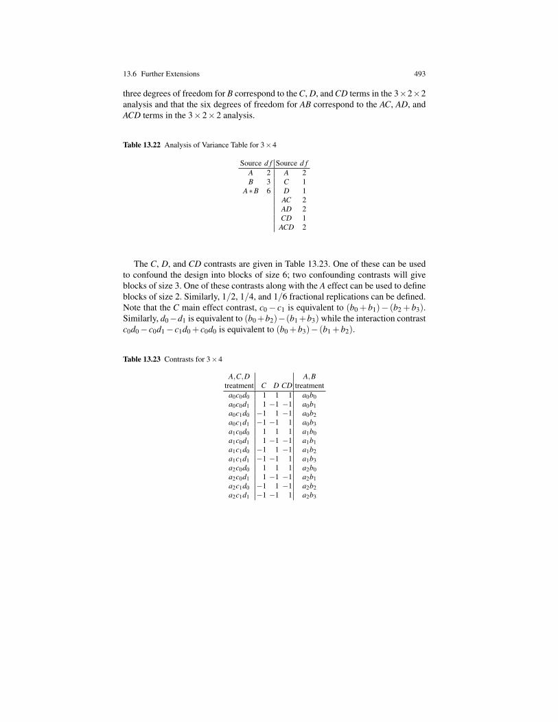
The C, D, and CD contrasts are given in Table 13.23. One of these can be usedto confound the design into blocks of size 6; two confounding contrasts will giveblocks of size 3. One of these contrasts along with the A effect can be used to defineblocks of size 2. Similarly, 1/2, 1/4, and 1/6 fractional replications can be defined.Note that the C main effect contrast, c0 − c1 is equivalent to (b0 + b1)− (b2 + b3).Similarly, d0−d1 is equivalent to (b0+b2)−(b1+b3) while the interaction contrastc0d0 − c0d1 − c1d0 + c0d0 is equivalent to (b0 +b3)− (b1 +b2).

Table 13.23 Contrasts for 3×4

A,C,D A,Btreatment C D CD treatment

a0c0d0 1 1 1 a0b0a0c0d1 1 −1 −1 a0b1a0c1d0 −1 1 −1 a0b2a0c1d1 −1 −1 1 a0b3a1c0d0 1 1 1 a1b0a1c0d1 1 −1 −1 a1b1a1c1d0 −1 1 −1 a1b2a1c1d1 −1 −1 1 a1b3a2c0d0 1 1 1 a2b0a2c0d1 1 −1 −1 a2b1a2c1d0 −1 1 −1 a2b2a2c1d1 −1 −1 1 a2b3

Documents

Chapter 13 Factorial Treatment Structures