Embed Size (px)
Citation preview
Chapter 12: Unemployment and Inflation
Yulei Luo
SEF of HKU
April 22, 2015
Luo, Y. (SEF of HKU) ECON2102CD/2220CD: Intermediate Macro April 22, 2015 1 / 29
Chapter Outline
Unemployment and Inflation: Is There a Trade-Off?
Macroeconomic Policy and the Phillips Curve
The Problem of Unemployment
The Problem of Inflation
Fighting Inflation: The Role of Inflationary Expectations
Luo, Y. (SEF of HKU) ECON2102CD/2220CD: Intermediate Macro April 22, 2015 2 / 29
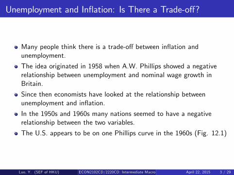
Unemployment and Inflation: Is There a Trade-off?
Many people think there is a trade-off between inflation andunemployment.
The idea originated in 1958 when A.W. Phillips showed a negativerelationship between unemployment and nominal wage growth inBritain.
Since then economists have looked at the relationship betweenunemployment and inflation.
In the 1950s and 1960s many nations seemed to have a negativerelationship between the two variables.
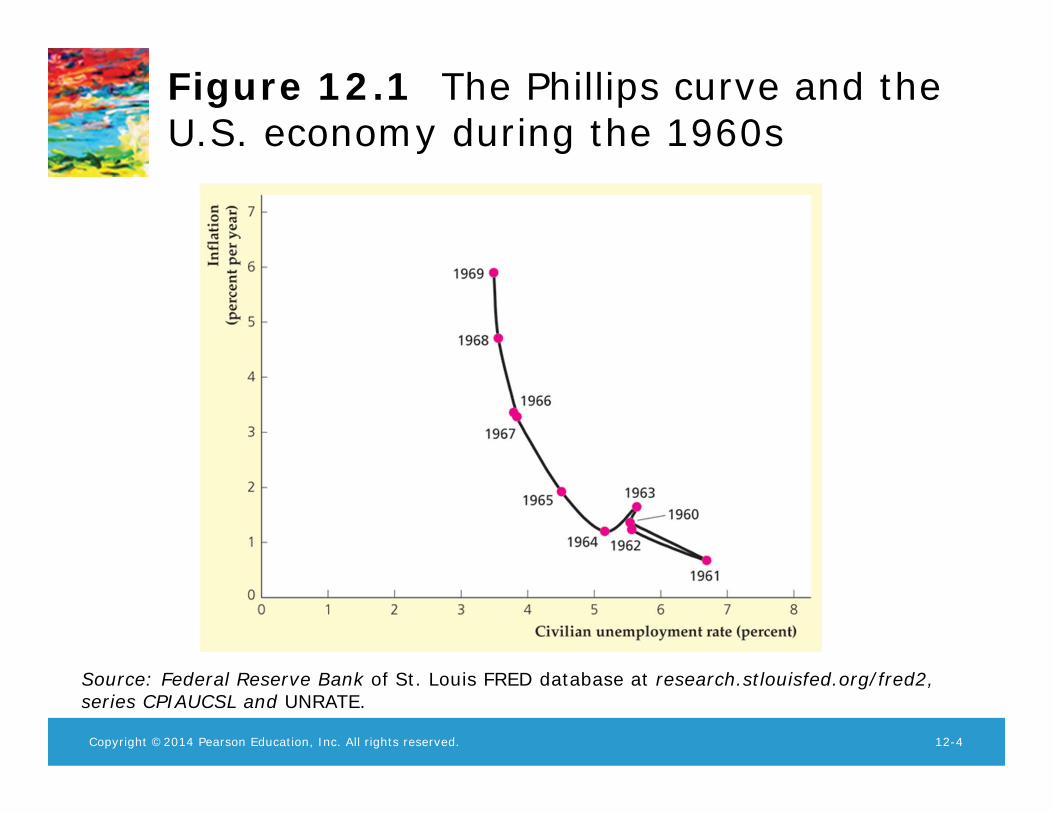
The U.S. appears to be on one Phillips curve in the 1960s (Fig. 12.1)
Luo, Y. (SEF of HKU) ECON2102CD/2220CD: Intermediate Macro April 22, 2015 3 / 29
Copyright ©2014 Pearson Education, Inc. All rights reserved. 12-4
Figure 12.1 The Phillips curve and the U.S. economy during the 1960s
Source: Federal Reserve Bank of St. Louis FRED database at research.stlouisfed.org/fred2, series CPIAUCSL and UNRATE.
(Conti.) This suggested that policymakers could choose thecombination of unemployment and inflation they most desired
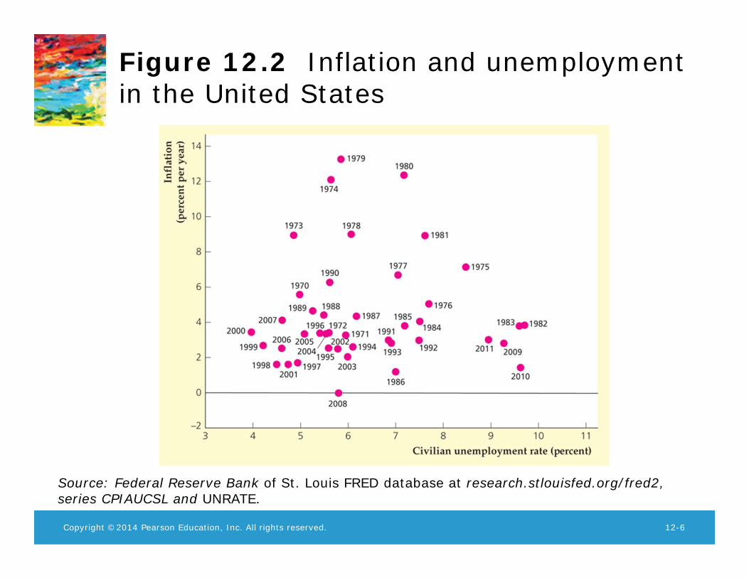
But the relationship fell apart in the following three decades (Fig.12.2)
The 1970s were a particularly bad period, with both high inflation andhigh unemployment, inconsistent with the Phillips curve.
Luo, Y. (SEF of HKU) ECON2102CD/2220CD: Intermediate Macro April 22, 2015 4 / 29
Copyright ©2014 Pearson Education, Inc. All rights reserved. 12-6
Figure 12.2 Inflation and unemployment in the United States
Source: Federal Reserve Bank of St. Louis FRED database at research.stlouisfed.org/fred2, series CPIAUCSL and UNRATE.
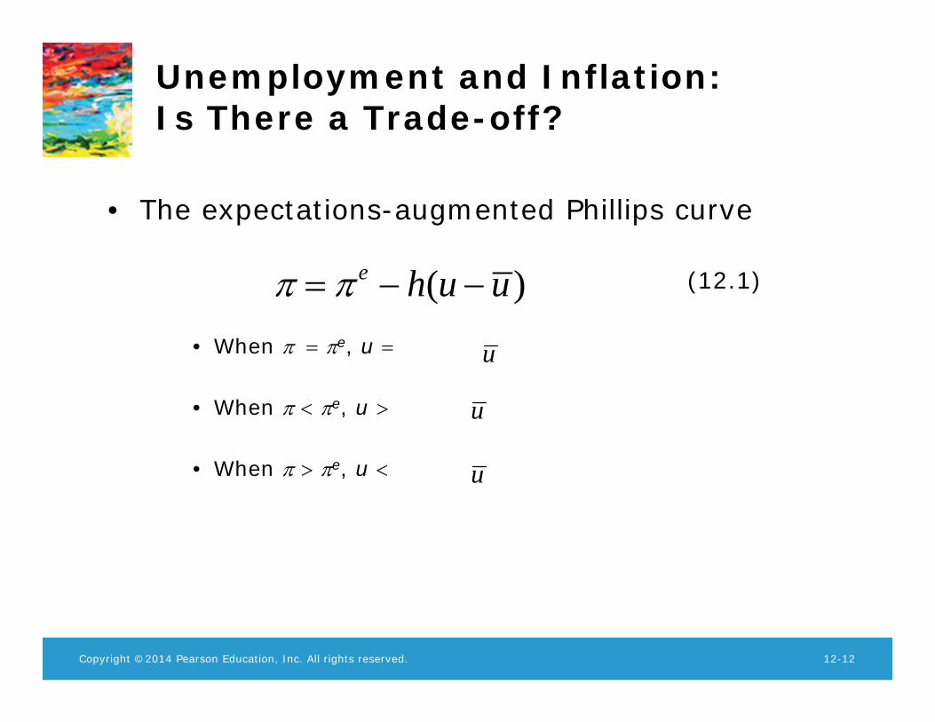
The expectations-augmented Phillips curve
Friedman and Phelps: The cyclical unemployment rate (the differencebetween actual and natural unemployment rates) depends only onunanticipated inflation (the difference between actual and expectedinflation):
This theory was made before the Phillips curve began breaking down inthe 1970s.It suggests that the relationship between inflation and theunemployment rate isn’t stable.
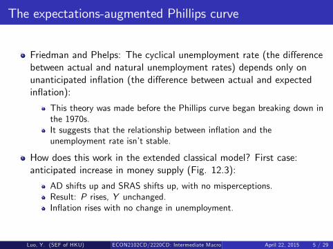
How does this work in the extended classical model? First case:anticipated increase in money supply (Fig. 12.3):
AD shifts up and SRAS shifts up, with no misperceptions.Result: P rises, Y unchanged.Inflation rises with no change in unemployment.
Luo, Y. (SEF of HKU) ECON2102CD/2220CD: Intermediate Macro April 22, 2015 5 / 29
Copyright ©2014 Pearson Education, Inc. All rights reserved. 12-9
Figure 12.3 Ongoing inflation in the extended classical model
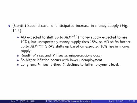
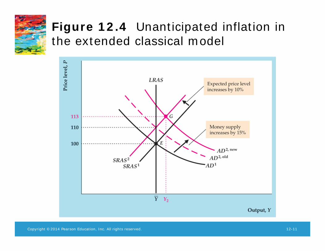
(Conti.) Second case: unanticipated increase in money supply (Fig.12.4):
AD expected to shift up to AD2,old (money supply expected to rise10%), but unexpectedly money supply rises 15%, so AD shifts furtherup to AD2,new SRAS shifts up based on expected 10% rise in moneysupplyResult: P rises and Y rises as misperceptions occurSo higher inflation occurs with lower unemploymentLong run: P rises further, Y declines to full-employment level.
Luo, Y. (SEF of HKU) ECON2102CD/2220CD: Intermediate Macro April 22, 2015 6 / 29
Copyright ©2014 Pearson Education, Inc. All rights reserved. 12-11
Figure 12.4 Unanticipated inflation in the extended classical model
Copyright ©2014 Pearson Education, Inc. All rights reserved. 12-12
Unemployment and Inflation: Is There a Trade-off?
• The expectations-augmented Phillips curve
(12.1)
• When π = πe, u =
• When π < πe, u >
• When π > πe, u < u
( )e h u uπ π= − −
u
u
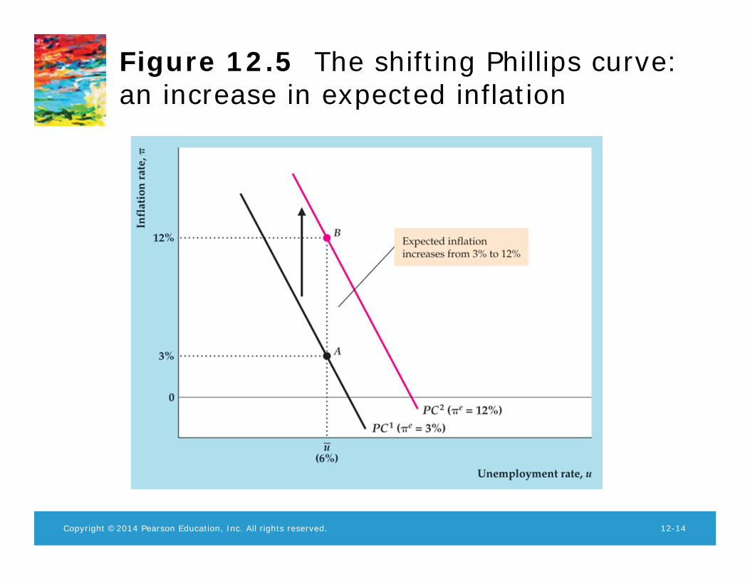
The shifting Phillips curve
The Phillips curve shows the relationship between unemployment andinflation for a given expected rate of inflation and natural rate ofunemployment.
Changes in the expected rate of inflation (Fig. 12.5):
For a given expected rate of inflation, the Phillips curve shows thetrade-off between cyclical unemployment and actual inflation.The Phillips curve is drawn such that π = πe when u = u.Higher expected inflation implies a higher Phillips curve.
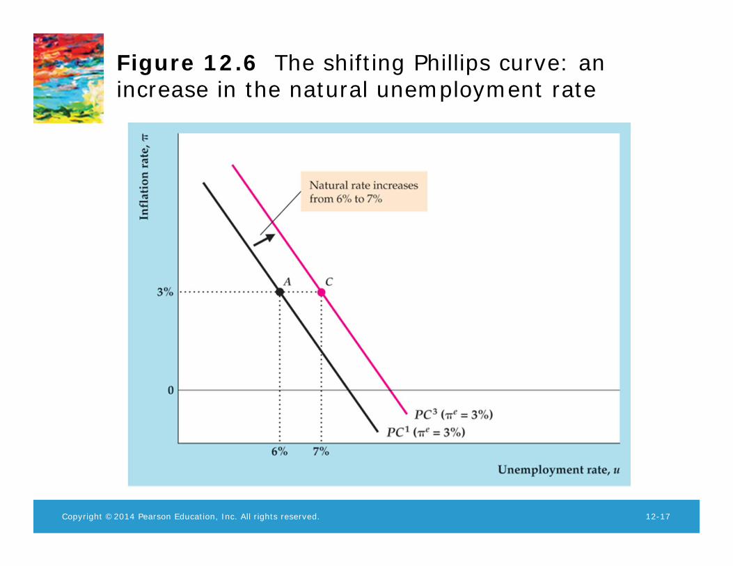
Changes in the natural rate of unemployment (Fig. 12.6):
For a given natural rate of unemployment, the Phillips curve shows thetrade-off between unemployment and unanticipated inflation.A higher natural rate of unemployment shifts the Phillips curve to theright.
Luo, Y. (SEF of HKU) ECON2102CD/2220CD: Intermediate Macro April 22, 2015 7 / 29
Copyright ©2014 Pearson Education, Inc. All rights reserved. 12-14
Figure 12.5 The shifting Phillips curve: an increase in expected inflation
Copyright ©2014 Pearson Education, Inc. All rights reserved. 12-17
Figure 12.6 The shifting Phillips curve: an increase in the natural unemployment rate
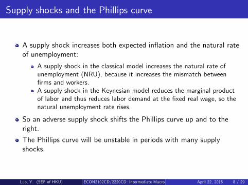
Supply shocks and the Phillips curve
A supply shock increases both expected inflation and the natural rateof unemployment:
A supply shock in the classical model increases the natural rate ofunemployment (NRU), because it increases the mismatch betweenfirms and workers.A supply shock in the Keynesian model reduces the marginal productof labor and thus reduces labor demand at the fixed real wage, so thenatural unemployment rate rises.
So an adverse supply shock shifts the Phillips curve up and to theright.
The Phillips curve will be unstable in periods with many supplyshocks.
Luo, Y. (SEF of HKU) ECON2102CD/2220CD: Intermediate Macro April 22, 2015 8 / 29

The shifting Phillips curve in practice
Why did the original Phillips curve relationship apply to manyhistorical cases?
The original relationship between inflation and unemployment holds upas long as expected inflation and NRU are approximately constant.This was true in the U.S. in the 1960s, so the Phillips curve appearedto be stable.
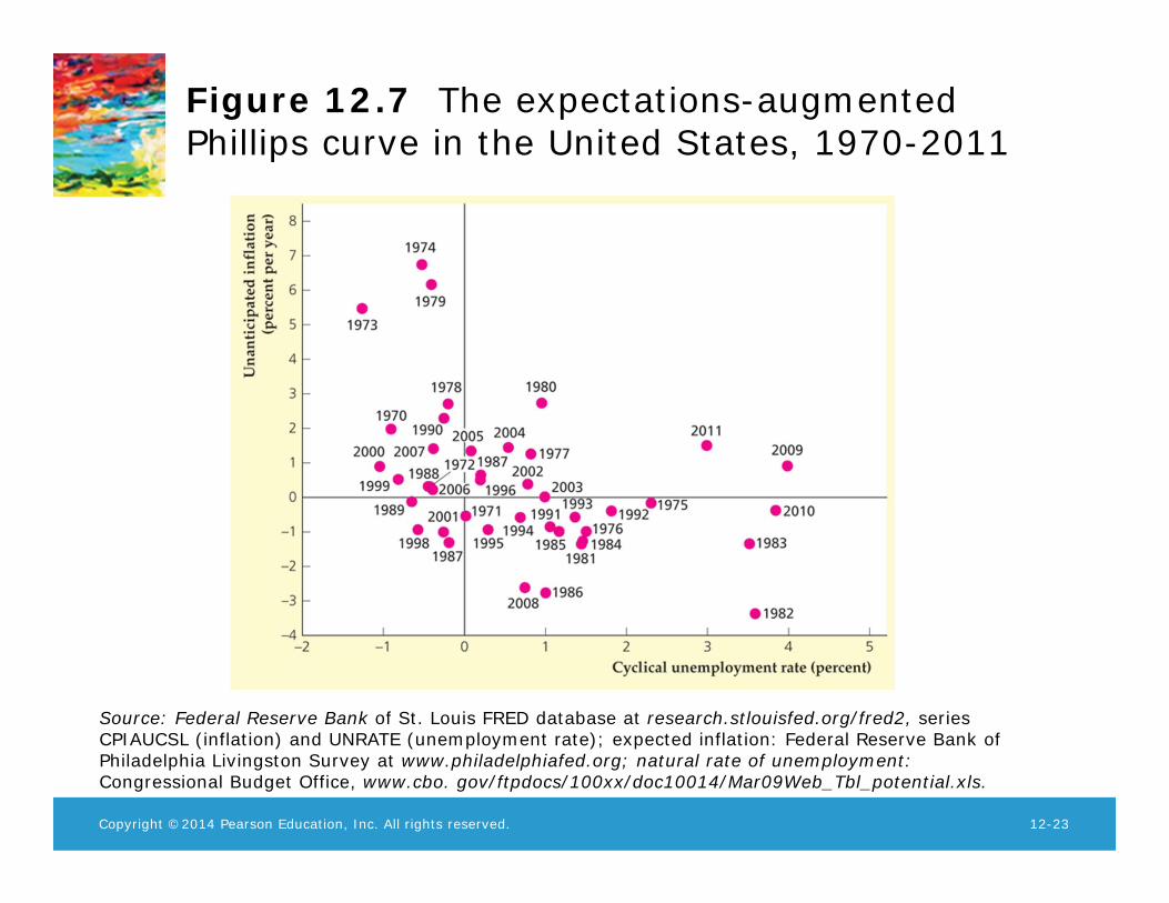
Why did the U.S. Phillips curve disappear after 1970?Both the expected inflation rate and the natural rate of unemploymentvaried considerably more in the 1970s than they did in the 1960s.Especially important were the oil price shocks of 1973− 1974 and1979− 1980.Also, the composition of the labor force changed in the 1970s and therewere other structural changes in the economy as well, raising NRU.Monetary policy was expansionary in the 1970s, leading to high andvolatile inflation.Plotting unanticipated inflation against cyclical unemployment shows afairly stable relationship since 1970 (Fig. 12.7).
Luo, Y. (SEF of HKU) ECON2102CD/2220CD: Intermediate Macro April 22, 2015 9 / 29
Copyright ©2014 Pearson Education, Inc. All rights reserved. 12-23
Figure 12.7 The expectations-augmented Phillips curve in the United States, 1970-2011
Source: Federal Reserve Bank of St. Louis FRED database at research.stlouisfed.org/fred2, series CPIAUCSL (inflation) and UNRATE (unemployment rate); expected inflation: Federal Reserve Bank of Philadelphia Livingston Survey at www.philadelphiafed.org; natural rate of unemployment: Congressional Budget Office, www.cbo. gov/ftpdocs/100xx/doc10014/Mar09Web_Tbl_potential.xls.
Macroeconomic Policy and the Phillips Curve
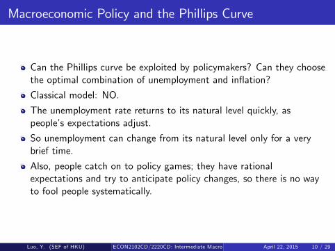
Can the Phillips curve be exploited by policymakers? Can they choosethe optimal combination of unemployment and inflation?
Classical model: NO.
The unemployment rate returns to its natural level quickly, aspeople’s expectations adjust.
So unemployment can change from its natural level only for a verybrief time.
Also, people catch on to policy games; they have rationalexpectations and try to anticipate policy changes, so there is no wayto fool people systematically.
Luo, Y. (SEF of HKU) ECON2102CD/2220CD: Intermediate Macro April 22, 2015 10 / 29
(Conti.) Keynesian model: YES, temporarily
The expected rate of inflation in the Phillips curve is the forecast ofinflation at the time the oldest sticky prices were set
It takes time for prices and expected prices to adjust, sounemployment may differ from the natural rate for some time
Luo, Y. (SEF of HKU) ECON2102CD/2220CD: Intermediate Macro April 22, 2015 11 / 29
In touch with data and research: The Lucas critique
When the rules of the game change, behavior changes.
For example, if batters in baseball were called out after two strikesinstead of three, they’d swing more often when they have one strikethan they do now.
Lucas applied this idea to macroeconomics, arguing that historicalrelationships between variables won’t hold up if there’s been a majorpolicy change.
The Phillips curve is a good example– it fell apart as soon aspolicymakers tried to exploit it.
Evaluating policy requires an understanding of how behavior willchange under the new policy, so both economic theory and empiricalanalysis are necessary.
Luo, Y. (SEF of HKU) ECON2102CD/2220CD: Intermediate Macro April 22, 2015 12 / 29
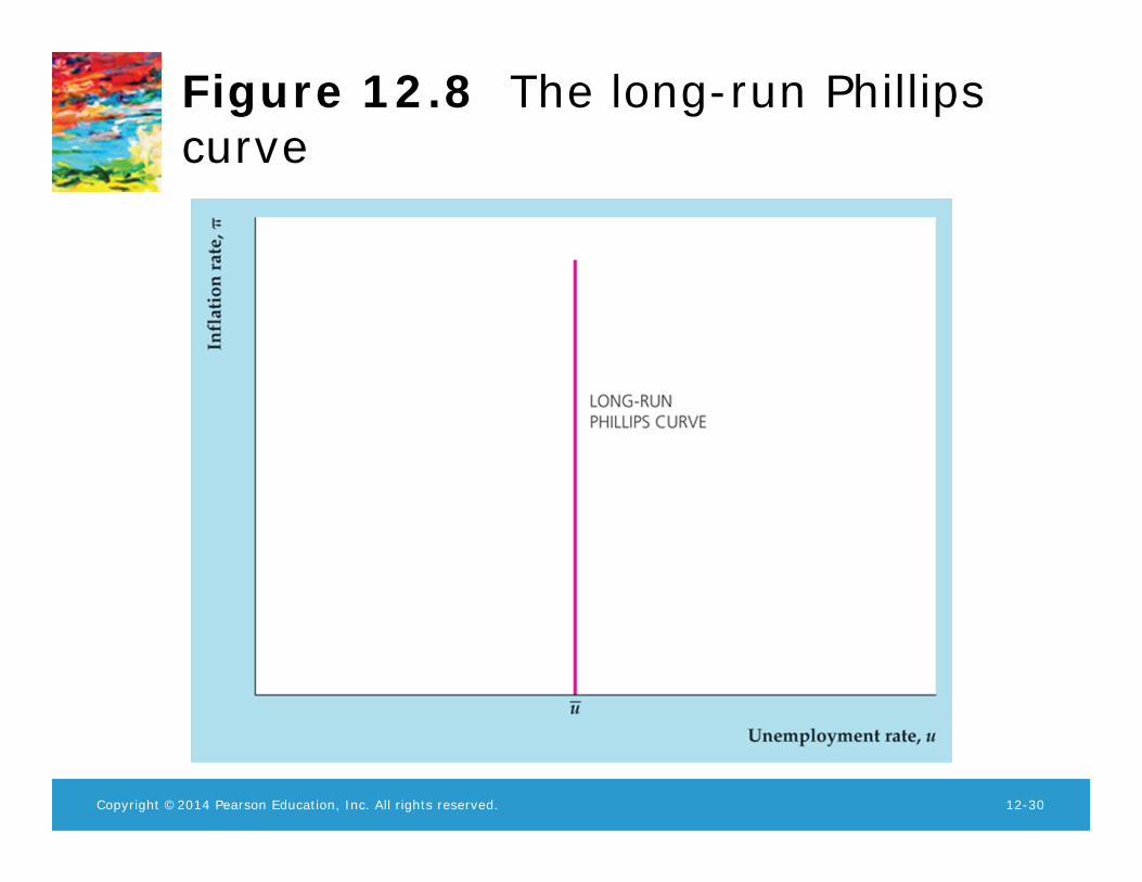
The long-run Phillips curve
Long run: the u = u for both Keynesians and classicals.
The long-run Phillips curve is vertical, since when π = πe , thenu = u. (Figure 12.8).
Changes in the level of money supply have no long-run real effects;changes in the growth rate of money supply have no long-run realeffects, either.
Even though expansionary policy may reduce unemployment onlytemporarily, policymakers may want to do so if, for example, timingeconomic booms right before elections helps them (or their politicalallies) get reelected.
Luo, Y. (SEF of HKU) ECON2102CD/2220CD: Intermediate Macro April 22, 2015 13 / 29
Copyright ©2014 Pearson Education, Inc. All rights reserved. 12-30
Figure 12.8 The long-run Phillips curve
The costs of unemployment
Loss in output from idle resources:
Workers lose income.Society pays for unemployment benefits and makes up lost tax revenue.Using Okun’s Law (each percentage point of cyclical unemployment isassociated with a loss equal to 2% of full-employment output), iffull-employment output is $17 trillion, each percentage point ofunemployment sustained for one year costs $340 billion.
Personal or psychological cost to workers and their families.
Especially important for those with long spells of unemployment.
There are some offsetting factors:
Unemployment leads to increased job search and acquiring new skills,which may lead to increased future output.Unemployed workers have increased leisure time, though most wouldn’tfeel that the increased leisure compensated them for being unemployed.
Luo, Y. (SEF of HKU) ECON2102CD/2220CD: Intermediate Macro April 22, 2015 14 / 29
The long-term behavior of the unemployment rate
The changing natural rate:
How do we calculate the NRU?CBO’s estimates: 6% today, similar to 1970s and 1980s; much higherthan it was in 1960s, 1990s, and 2000s.In the 1980s and 1990s, demographic forces reduced NRU (Fig. 12.9)The proportion of the labor force aged 16—24 years fell from 25% in1980 to 16% in 1998.Research by Shimer showed this is the main reason for the fall in NRU.
Luo, Y. (SEF of HKU) ECON2102CD/2220CD: Intermediate Macro April 22, 2015 15 / 29
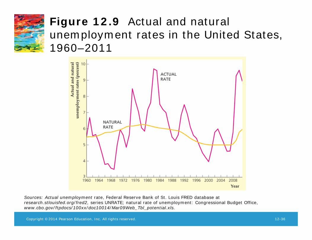
Copyright ©2014 Pearson Education, Inc. All rights reserved. 12-36
Figure 12.9 Actual and natural unemployment rates in the United States, 1960–2011
Sources: Actual unemployment rate, Federal Reserve Bank of St. Louis FRED database at research.stlouisfed.org/fred2, series UNRATE; natural rate of unemployment: Congressional Budget Office, www.cbo.gov/ftpdocs/100xx/doc10014/Mar09Web_Tbl_potential.xls.
(Conti.) Some economists think NRU was 4.5% or even lower in the1990s and 2000s. The labor market became more effi cient atmatching workers and jobs, reducing frictional and structuralunemployment. Temporary help agencies became prominent, helpingthe matching process and reducing the natural rate of unemployment
Increased labor productivity may increase NRU. If increases in realwages lag changes in productivity, firms hire more workers and NRUwill decline temporarily. Ball and Mankiw found evidence supportingthis hypothesis in the 1990s
Luo, Y. (SEF of HKU) ECON2102CD/2220CD: Intermediate Macro April 22, 2015 16 / 29
Measuring the natural rate of unemployment
Policymakers need a measure of NRU to use the unemployment ratefor setting policy.
Economists disagree about how to measure NRU and the CBO hasoften revised its measure.
Staiger, Stock, and Watson found that NRU cannot be measuredprecisely with econometric methods, as the confidence interval is verylarge.
What should policymakers do in response to uncertainty about NRU?
They may wish to be less aggressive with policy than they would be ifthey knew the natural rate more precisely.Research (Orphanides-Williams) suggests that the rise of inflation inthe 1970s can be blamed on bad estimates of the natural rate.
Luo, Y. (SEF of HKU) ECON2102CD/2220CD: Intermediate Macro April 22, 2015 17 / 29
The costs of inflation (Perfectly anticipated inflation)
No effects if all prices and wages keep up with inflation.
Even returns on assets may rise exactly with inflation.
Shoe-leather costs: People spend resources to economize on currencyholdings; the estimated cost of 10% inflation is 0.3% of GNP.
Menu costs: the costs of changing prices (but technology maymitigate this somewhat).
Luo, Y. (SEF of HKU) ECON2102CD/2220CD: Intermediate Macro April 22, 2015 18 / 29
Unanticipated inflation
Unanticipated inflation is π − πe . Realized real returns differ fromexpected real returns:
Expected: r = i − πe
Actual: r = i − π
That is, actual r differs from expected r by πe − π.
Numerical example: i = 6%,πe = 4%, so expected r = 2%; ifπ = 6%, actual r = 0%; if π = 2%, actual r = 4%.
Luo, Y. (SEF of HKU) ECON2102CD/2220CD: Intermediate Macro April 22, 2015 19 / 29
(Conti.) Similar effect on wages and salaries. Result: transfer ofwealth
From lenders to borrowers when π > πe
From borrowers to lenders when π < πe
So people want to avoid risk of unanticipated inflation. They spendresources to forecast inflation.
Loss of valuable signals provided by prices:
Confusion over changes in aggregate prices vs. changes in relativeprices.People expend resources to extract correct signals from prices.
Luo, Y. (SEF of HKU) ECON2102CD/2220CD: Intermediate Macro April 22, 2015 20 / 29
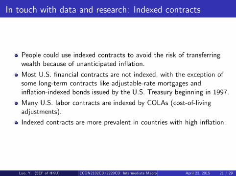
In touch with data and research: Indexed contracts
People could use indexed contracts to avoid the risk of transferringwealth because of unanticipated inflation.
Most U.S. financial contracts are not indexed, with the exception ofsome long-term contracts like adjustable-rate mortgages andinflation-indexed bonds issued by the U.S. Treasury beginning in 1997.
Many U.S. labor contracts are indexed by COLAs (cost-of-livingadjustments).
Indexed contracts are more prevalent in countries with high inflation.
Luo, Y. (SEF of HKU) ECON2102CD/2220CD: Intermediate Macro April 22, 2015 21 / 29
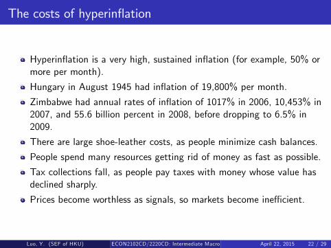
The costs of hyperinflation
Hyperinflation is a very high, sustained inflation (for example, 50% ormore per month).
Hungary in August 1945 had inflation of 19,800% per month.
Zimbabwe had annual rates of inflation of 1017% in 2006, 10,453% in2007, and 55.6 billion percent in 2008, before dropping to 6.5% in2009.
There are large shoe-leather costs, as people minimize cash balances.
People spend many resources getting rid of money as fast as possible.
Tax collections fall, as people pay taxes with money whose value hasdeclined sharply.
Prices become worthless as signals, so markets become ineffi cient.
Luo, Y. (SEF of HKU) ECON2102CD/2220CD: Intermediate Macro April 22, 2015 22 / 29
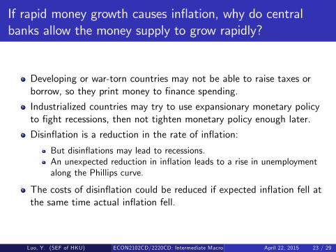
If rapid money growth causes inflation, why do centralbanks allow the money supply to grow rapidly?
Developing or war-torn countries may not be able to raise taxes orborrow, so they print money to finance spending.
Industrialized countries may try to use expansionary monetary policyto fight recessions, then not tighten monetary policy enough later.
Disinflation is a reduction in the rate of inflation:
But disinflations may lead to recessions.An unexpected reduction in inflation leads to a rise in unemploymentalong the Phillips curve.
The costs of disinflation could be reduced if expected inflation fell atthe same time actual inflation fell.
Luo, Y. (SEF of HKU) ECON2102CD/2220CD: Intermediate Macro April 22, 2015 23 / 29
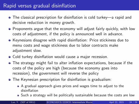
Rapid versus gradual disinflation
The classical prescription for disinflation is cold turkey– a rapid anddecisive reduction in money growth.
Proponents argue that the economy will adjust fairly quickly, with lowcosts of adjustment, if the policy is announced well in advance.
Keynesians disagree with rapid disinflation: Price stickiness due tomenu costs and wage stickiness due to labor contracts makeadjustment slow.
Cold turkey disinflation would cause a major recession.
The strategy might fail to alter inflation expectations, because if thecosts of the policy are high (because the economy goes intorecession), the government will reverse the policy
The Keynesian prescription for disinflation is gradualism:
A gradual approach gives prices and wages time to adjust to thedisinflationSuch a strategy will be politically sustainable because the costs are low
Luo, Y. (SEF of HKU) ECON2102CD/2220CD: Intermediate Macro April 22, 2015 24 / 29
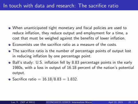
In touch with data and research: The sacrifice ratio
When unanticipated tight monetary and fiscal policies are used toreduce inflation, they reduce output and employment for a time, acost that must be weighed against the benefits of lower inflation.
Economists use the sacrifice ratio as a measure of the costs.
The sacrifice ratio is the number of percentage points of output lostin reducing inflation by one percentage point.
Ball’s study: U.S. inflation fell by 8.83 percentage points in the early1980s, with a loss in output of 16.18 percent of the nation’s potentialoutput.
Sacrifice ratio = 16.18/8.83 = 1.832.
Luo, Y. (SEF of HKU) ECON2102CD/2220CD: Intermediate Macro April 22, 2015 25 / 29
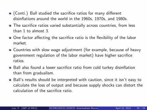
(Conti.) Ball studied the sacrifice ratios for many differentdisinflations around the world in the 1960s, 1970s, and 1980s.
The sacrifice ratios varied substantially across countries, from lessthan 1 to almost 3.
One factor affecting the sacrifice ratio is the flexibility of the labormarket.
Countries with slow wage adjustment (for example, because of heavygovernment regulation of the labor market) have higher sacrificeratios.
Ball also found a lower sacrifice ratio from cold turkey disinflationthan from gradualism.
Ball’s results should be interpreted with caution, since it isn’t easy tocalculate the loss of output and because supply shocks can distort thecalculation of the sacrifice ratio.
Luo, Y. (SEF of HKU) ECON2102CD/2220CD: Intermediate Macro April 22, 2015 26 / 29
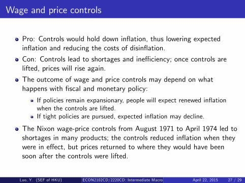
Wage and price controls
Pro: Controls would hold down inflation, thus lowering expectedinflation and reducing the costs of disinflation.
Con: Controls lead to shortages and ineffi ciency; once controls arelifted, prices will rise again.
The outcome of wage and price controls may depend on whathappens with fiscal and monetary policy:
If policies remain expansionary, people will expect renewed inflationwhen the controls are lifted.If tight policies are pursued, expected inflation may decline.
The Nixon wage-price controls from August 1971 to April 1974 led toshortages in many products; the controls reduced inflation when theywere in effect, but prices returned to where they would have beensoon after the controls were lifted.
Luo, Y. (SEF of HKU) ECON2102CD/2220CD: Intermediate Macro April 22, 2015 27 / 29
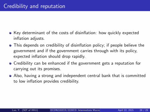
Credibility and reputation
Key determinant of the costs of disinflation: how quickly expectedinflation adjusts.
This depends on credibility of disinflation policy; if people believe thegovernment and if the government carries through with its policy,expected inflation should drop rapidly.
Credibility can be enhanced if the government gets a reputation forcarrying out its promises.
Also, having a strong and independent central bank that is committedto low inflation provides credibility.
Luo, Y. (SEF of HKU) ECON2102CD/2220CD: Intermediate Macro April 22, 2015 28 / 29
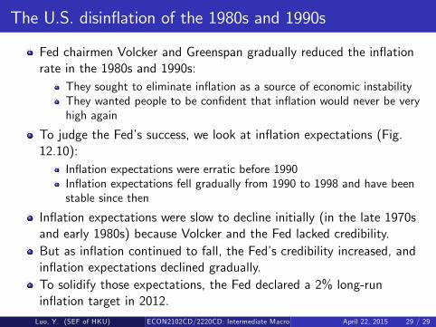
The U.S. disinflation of the 1980s and 1990s
Fed chairmen Volcker and Greenspan gradually reduced the inflationrate in the 1980s and 1990s:
They sought to eliminate inflation as a source of economic instabilityThey wanted people to be confident that inflation would never be veryhigh again
To judge the Fed’s success, we look at inflation expectations (Fig.12.10):
Inflation expectations were erratic before 1990Inflation expectations fell gradually from 1990 to 1998 and have beenstable since then
Inflation expectations were slow to decline initially (in the late 1970sand early 1980s) because Volcker and the Fed lacked credibility.But as inflation continued to fall, the Fed’s credibility increased, andinflation expectations declined gradually.To solidify those expectations, the Fed declared a 2% long-runinflation target in 2012.Luo, Y. (SEF of HKU) ECON2102CD/2220CD: Intermediate Macro April 22, 2015 29 / 29
Copyright ©2014 Pearson Education, Inc. All rights reserved. 12-63
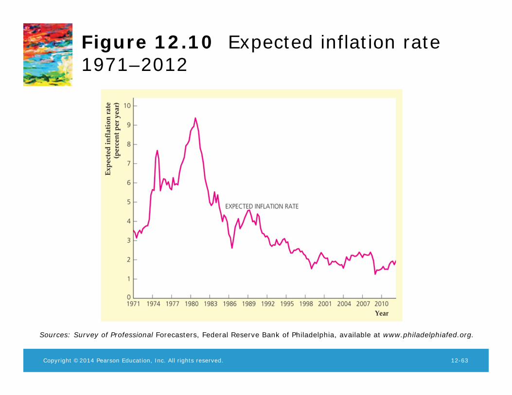
Figure 12.10 Expected inflation rate 1971–2012
Sources: Survey of Professional Forecasters, Federal Reserve Bank of Philadelphia, available at www.philadelphiafed.org.