Chapter 12 – Simple Harmonic Motionphysics.bu.edu/~duffy/ns544_summer2009_notes02/NS544_online1.pdf · Chapter 12 – Simple Harmonic Motion Page 3 Answer to Essential Question

Chapter 12 – Simple Harmonic Motion Page 1

Chapter 12 – Simple Harmonic Motion We will now turn our attention to oscillating systems, such as an object bobbing up and down on the end of a spring, or a child swinging on a playground swing. We’ll focus on a simple model, in which the total mechanical energy is constant. This is a reasonable starting point for most oscillating systems. Our own starting point, however, will be to consider how to incorporate springs into our force and energy perspectives. The photograph shows a time-sequence of a metronome. Understanding the motion of such oscillating systems is the main focus of this chapter. Photo credit: Libby Chapman / iStockPhoto.

12-1 Hooke’s Law We probably all have some experience with springs. One observation we can make is that

it doesn’t take much force to stretch or compress a spring a small amount, but the more we try to compress or stretch it the more force we need. We’ll use a model of an ideal spring, in which the magnitude of the force associated with stretching or compressing the spring is proportional to the distance the spring is stretched or compressed.

The equation describing the proportionality of the spring force with the displacement of

the end of the spring from its natural length is known as Hooke’s Law. SpringF k x= −v v . (Equation 12.1: Hooke’s Law)

The negative sign is associated with the restoring nature of the force. When you displace

the end of the spring in one direction from its equilibrium position the spring applies a force in the opposite direction, essentially in an attempt to return the system toward the equilibrium position (the position where the spring is at its natural length, neither stretched nor compressed).

The k in the Hooke’s Law equation is known as the spring constant. This is a measure of

the stiffness of the spring. If you have two different springs and you stretch them the same amount from equilibrium. The one that requires more force to maintain that stretch has the larger spring constant. Figure 12.1 shows the Hooke’s Law relationship as a graph of force as a function of the amount of compression or stretch of a particular spring from its natural length.

Figure 12.1: A graph of the force applied by a particular spring as a function of the displacement of the end of the spring from its equilibrium position.

The Hooke’s Law relationship is illustrated in Figure

12.2, where x = 0 means the spring is neither stretched nor compressed from its natural length. A block attached to spring has been released and is oscillating on a frictionless surface. Free-body diagrams are shown in Figure 12.2, illustrating how the force exerted by the spring on the block depends on the displacement of the end of the spring from its equilibrium position.


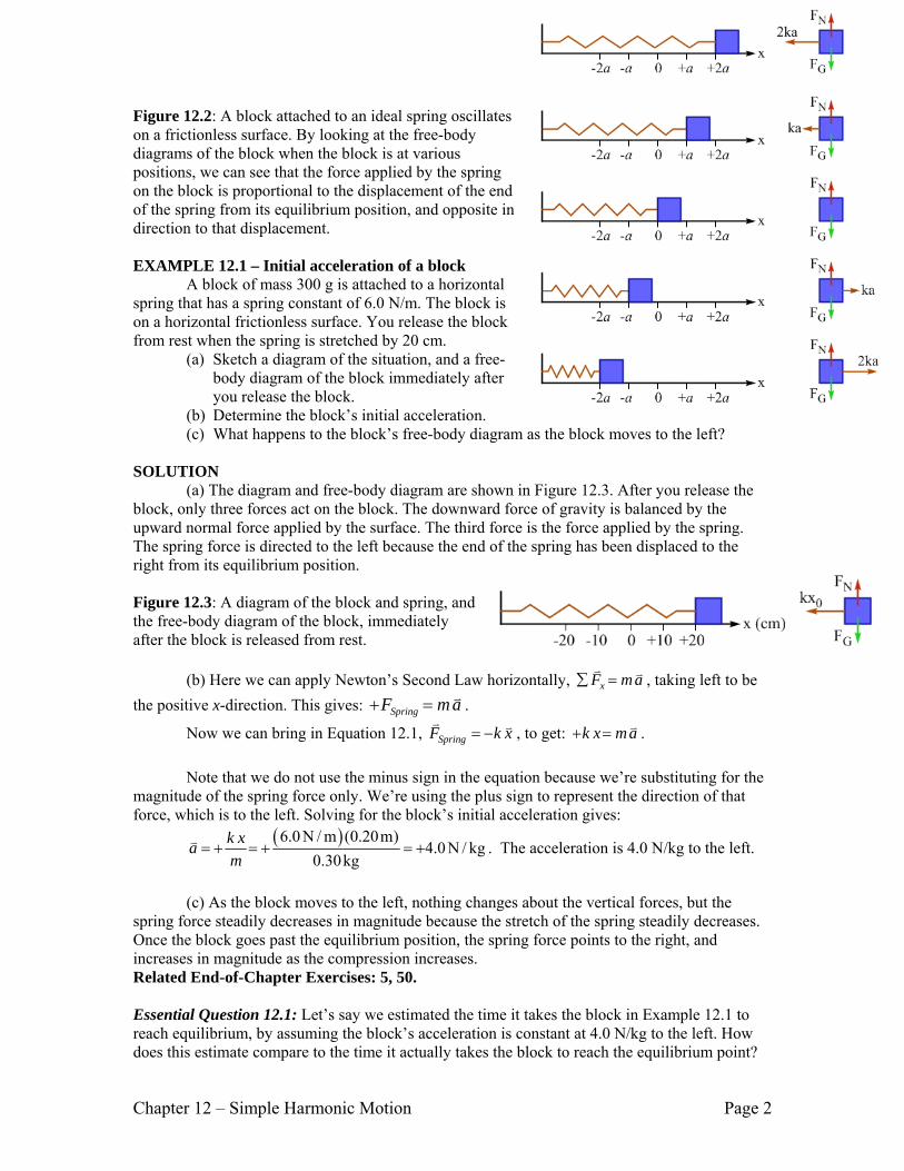
Figure 12.2: A block attached to an ideal spring oscillates on a frictionless surface. By looking at the free-body diagrams of the block when the block is at various positions, we can see that the force applied by the spring on the block is proportional to the displacement of the end of the spring from its equilibrium position, and opposite in direction to that displacement.

EXAMPLE 12.1 – Initial acceleration of a block

A block of mass 300 g is attached to a horizontal spring that has a spring constant of 6.0 N/m. The block is on a horizontal frictionless surface. You release the block from rest when the spring is stretched by 20 cm.

(a) Sketch a diagram of the situation, and a free-body diagram of the block immediately after you release the block.

(b) Determine the block’s initial acceleration. (c) What happens to the block’s free-body diagram as the block moves to the left?

SOLUTION (a) The diagram and free-body diagram are shown in Figure 12.3. After you release the

block, only three forces act on the block. The downward force of gravity is balanced by the upward normal force applied by the surface. The third force is the force applied by the spring. The spring force is directed to the left because the end of the spring has been displaced to the right from its equilibrium position.

Figure 12.3: A diagram of the block and spring, and the free-body diagram of the block, immediately after the block is released from rest.

(b) Here we can apply Newton’s Second Law horizontally, xF ma∑ =

v v , taking left to be the positive x-direction. This gives: SpringF ma+ = v .

Now we can bring in Equation 12.1, SpringF k x= −v v , to get: k x ma+ = v .

Note that we do not use the minus sign in the equation because we’re substituting for the

magnitude of the spring force only. We’re using the plus sign to represent the direction of that force, which is to the left. Solving for the block’s initial acceleration gives:

( )6.0 N / m (0.20m)4.0 N / kg

0.30kgk xam

= + = + = +v . The acceleration is 4.0 N/kg to the left.

(c) As the block moves to the left, nothing changes about the vertical forces, but the

spring force steadily decreases in magnitude because the stretch of the spring steadily decreases. Once the block goes past the equilibrium position, the spring force points to the right, and increases in magnitude as the compression increases. Related End-of-Chapter Exercises: 5, 50. Essential Question 12.1: Let’s say we estimated the time it takes the block in Example 12.1 to reach equilibrium, by assuming the block’s acceleration is constant at 4.0 N/kg to the left. How does this estimate compare to the time it actually takes the block to reach the equilibrium point?


Answer to Essential Question 12.1: This estimated time is less than the actual time. The closer the block gets to the equilibrium position, the smaller the force that is exerted on it by the spring, and the smaller the magnitude of the block’s acceleration. Because the block generally has a smaller acceleration than the acceleration we used in the constant-acceleration analysis, it will take longer to reach equilibrium than the time you calculated with the constant-acceleration analysis. Thus, remember not to use constant-acceleration equations in harmonic motion situations! We’ll learn how to calculate exact times in sections 12-4 to 12-6.

12-2 Springs and Energy Conservation Now that we have seen how to incorporate springs into a force perspective, let’s go on to

consider how to fit springs into what we know about energy.

EXPLORATION 12.2 – Another kind of potential energy

Step 1 – Attach a block to a spring, and position the block so that the spring is stretched. Let’s neglect friction, so when you release the block from rest it oscillates back and forth about the equilibrium position. What is going on with the energy of the system as the block oscillates? As the block oscillates, its speed increases from zero to some maximum value, then decreases to zero again, and keeps doing this over and over. The kinetic energy of the system does exactly the same thing, since it is proportional to the square of this speed. Where does the energy go when the kinetic energy decreases, and where does it comes from when the kinetic energy increases?

The energy is stored as potential energy in the spring. This is similar to what happens

when we throw a ball up into the air. As the ball rises, the ball’s loss of kinetic energy is offset by the gain in the gravitational potential energy of the Earth-ball system, and then that potential energy is transformed back into kinetic energy. Compressed or stretched springs also store potential energy. Such energy is known as elastic potential energy.

Step 2 - Consider the graph of force, as a function of the displacement of the end of the spring, shown in Figure 12.4. As we did in chapter 6, defining the change in gravitational potential energy to be the negative of the work done by gravity on an object, find an expression for the change in elastic potential energy as the end of the spring is displaced from its equilibrium position (x = 0) to some arbitrary final position x. Make use of the fact that work is the area under the force-versus-position graph in Figure 12.5.

Figure 12.4: The work done by a spring when its end is displaced from the equilibrium position to a point x away from equilibrium is represented by the shaded area in the graph.

The area in question is that of the right-angled triangle

shown in Figure 12.4. The area is negative because the force is negative the entire time. The area under the curve is given by:

21 1 1area base height ( )2 2 2

x kx kx= − × = − = − .

This area represents the work done by the spring. This work is negative because the spring force is opposite in direction to the displacement. Because eU∆ , the change in the elastic

potential energy, is the negative of the work, we have 212eU kx∆ = in this case.


Step 3 – How much elastic potential energy is stored in the spring when the spring is at its natural length? None. If we attach a block to such a spring and release the block from rest, no motion occurs because the system is at equilibrium. There is no transformation of elastic potential energy into kinetic energy because the system has no elastic potential energy when the spring is at its natural length – the equilibrium position is the zero for elastic potential energy.

Step 4 – Combine the results from parts 2 and 3 to determine the expression for the elastic potential energy stored in a spring when the end of the spring is displaced a distance x from its equilibrium position. In step 3 we found the change in elastic potential energy in displacing the end of the spring from its equilibrium position to a point x away from equilibrium to be

212eU kx∆ = . This change in elastic potential energy is equal to the final elastic potential energy

minus the initial elastic potential energy. However, we found the initial elastic potential energy to be zero in step 3, which means the expression for elastic potential energy is simply:

212eU kx= . (Equation 12.2: Elastic potential energy)

Key ideas: Compressed or stretched springs store energy – this is known as elastic potential

energy. For an ideal spring the elastic potential energy is 212eU kx= .

Related End-of-Chapter Exercises: 41, 42.

Now that we know the form of the elastic potential energy equation, we can incorporate

springs into the conservation of energy equation we first used in chapter 7: ffncii UKWUK +=++ . (Equation 7.1)

Graphs of the energies as a function of position are interesting. Consider a block attached

to a spring. The block is oscillating back and forth on a frictionless surface, so the total mechanical energy stays constant. An easy way to graph the kinetic energy is to exploit energy conservation, E K U= + . Solving for the kinetic energy as a function of position gives:

212

K E U E k x= − = − .

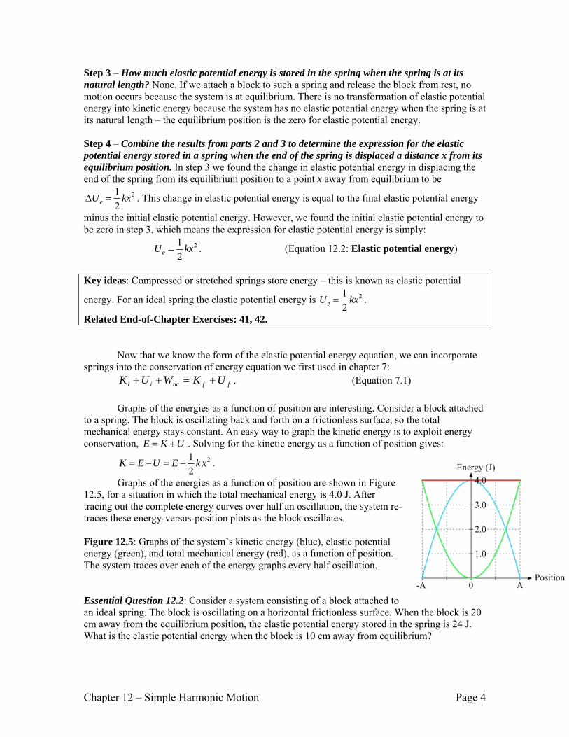
Graphs of the energies as a function of position are shown in Figure 12.5, for a situation in which the total mechanical energy is 4.0 J. After tracing out the complete energy curves over half an oscillation, the system re-traces these energy-versus-position plots as the block oscillates.

Figure 12.5: Graphs of the system’s kinetic energy (blue), elastic potential energy (green), and total mechanical energy (red), as a function of position. The system traces over each of the energy graphs every half oscillation.

Essential Question 12.2: Consider a system consisting of a block attached to an ideal spring. The block is oscillating on a horizontal frictionless surface. When the block is 20 cm away from the equilibrium position, the elastic potential energy stored in the spring is 24 J. What is the elastic potential energy when the block is 10 cm away from equilibrium?


Answer to Essential Question 12.2: To answer this question, we can use the fact that the elastic potential energy is proportional to 2x . Doubling x, the distance from equilibrium, increases the elastic potential energy by a factor of 4. Thus, the elastic potential energy is 6 J when x = 10 cm.

12-3 An Example Involving Springs and Energy

EXAMPLE 12.3 – A fast-moving block (a) A block of mass m, which rests on a horizontal frictionless surface, is attached to an

ideal horizontal spring. The block is released from rest when the spring is stretched by a distance A from its natural length. What is the block’s maximum speed during the ensuing oscillations?

(b) If the block is released from rest when the spring is stretched by 2A instead, how does the block’s maximum speed change?

SOLUTION

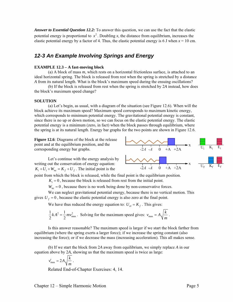
(a) Let’s begin, as usual, with a diagram of the situation (see Figure 12.6). When will the block achieve its maximum speed? Maximum speed corresponds to maximum kinetic energy, which corresponds to minimum potential energy. The gravitational potential energy is constant, since there is no up or down motion, so we can focus on the elastic potential energy. The elastic potential energy is a minimum (zero, in fact) when the block passes through equilibrium, where the spring is at its natural length. Energy bar graphs for the two points are shown in Figure 12.6.

Figure 12.6: Diagrams of the block at the release point and at the equilibrium position, and the corresponding energy bar graphs.

Let’s continue with the energy analysis by

writing out the conservation of energy equation: i i nc f fK U W K U+ + = + . The initial point is the

point from which the block is released, while the final point is the equilibrium position. 0iK = , because the block is released from rest from the initial point. 0ncW = , because there is no work being done by non-conservative forces.

We can neglect gravitational potential energy, because there is no vertical motion. This gives 0fU = , because the elastic potential energy is also zero at the final point.

We have thus reduced the energy equation to: ei fU K= . This gives:

2 2max

1 12 2

k A mv= . Solving for the maximum speed gives: maxkv Am

= .

Is this answer reasonable? The maximum speed is larger if we start the block farther from

equilibrium (where the spring exerts a larger force); if we increase the spring constant (also increasing the force); or if we decrease the mass (increasing acceleration). This all makes sense.

(b) If we start the block from 2A away from equilibrium, we simply replace A in our

equation above by 2A, showing us that the maximum speed is twice as large:

max 2 kv Am

′ = .



We can make an interesting generalization based on further analysis of the situation in Example 12.3. Take two blocks, one red and one blue but otherwise identical, and two identical springs. Attach each block to one of the springs, and place these two block-spring systems on frictionless horizontal surfaces. As shown in Figure 12.7, we will release one block from rest from a distance A from equilibrium and the other from a distance 2A from equilibrium. If the blocks are released simultaneously, which block reaches the equilibrium point first?

Figure 12.7: Identical blocks attached to identical springs. The blocks are released from rest simultaneously. Block 2, in red, is released from a distance 2A from equilibrium. Block 1 is released from a distance A from equilibrium. The initial free-body diagrams are also shown.

Block 2 has an initial acceleration twice as large

as that of block 1, because block 2 experiences a net force that is twice as large as that experienced by block 1. The accelerations steadily decrease, because the spring force decreases as the blocks get closer to equilibrium, but we can neglect this change if we choose a time interval that is sufficiently small.

At the end of this time interval, t∆ , what is the speed of each block? We’re choosing a

small time interval so that we can apply a constant-acceleration analysis. Remembering that the blocks are released from rest, so 0iv = , we have:

for block 1, in blue, 1 1 1 1iv v a t a t= + ∆ = ∆v v v v ; for block 2, in red, 2 2 2 2 1 12 2iv v a t a t a t v= + ∆ = ∆ = ∆ =v v v v v v . What about the distance each block travels? Here we can apply another constant

acceleration equation:

for block 1 ( ) ( )2 21 1 1 1

1 12 2ix v t a t a t∆ = ∆ + ∆ = ∆v v v v ;

for block 2 ( ) ( ) ( )2 2 22 02 2 2 1 1

1 1 1 (2 ) 22 2 2

x v t a t a t a t x∆ = ∆ + ∆ = ∆ = ∆ = ∆v v v v v v .

At the end of the time interval block 1 is 1A x−∆ from equilibrium and block 2 is exactly twice as far from equilibrium as block 1, at ( )1 12 2 2A x A x− ∆ = −∆ from equilibrium. Thus, after this small time interval has passed block 2 is still twice as far from equilibrium as block 1, its velocity is twice as large, and its acceleration is twice as large. We could keep the process going, following the two blocks as time goes by, and we would find this always to be true, the block 2’s velocity, acceleration, and displacement from equilibrium, is always double that of block 2. This is true at all times, even after the blocks pass through their equilibrium positions to the far side of equilibrium.

This leads to an amazing conclusion – that the two blocks take exactly the same time to

reach equilibrium (and to complete one full cycle of an oscillation). This is because block 2 experiences twice the displacement of block 1, but its average velocity is also twice as large. Since the time is the distance divided by the average velocity these factors of two cancel out.

Essential Question 12.3: Above we analyzed the situation of two identical (aside from color) blocks, oscillating on identical springs, and found the time to reach equilibrium (or to complete one full oscillation) to be the same. Was that just a coincidence that happened to work out because the starting displacements from equilibrium were in a 2:1 ratio, or can we generalize and say that the time is the same no matter where the block is released?


Answer to Essential Question 12.3: In fact, this result is generally true. As long as the spring is ideal, then the time it takes a block to move through one complete oscillation is independent of the amplitude of the oscillation. The amplitude is defined as the maximum distance an object gets from its equilibrium position during its oscillatory motion.

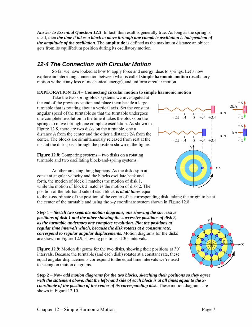
12-4 The Connection with Circular Motion So far we have looked at how to apply force and energy ideas to springs. Let’s now

explore an interesting connection between what is called simple harmonic motion (oscillatory motion without any loss of mechanical energy), and uniform circular motion. EXPLORATION 12.4 – Connecting circular motion to simple harmonic motion

Take the two spring-block systems we investigated at the end of the previous section and place them beside a large turntable that is rotating about a vertical axis. Set the constant angular speed of the turntable so that the turntable undergoes one complete revolution in the time it takes the blocks on the springs to move through one complete oscillation. As shown in Figure 12.8, there are two disks on the turntable, one a distance A from the center and the other a distance 2A from the center. The blocks are simultaneously released from rest at the instant the disks pass through the position shown in the figure.

Figure 12.8: Comparing systems – two disks on a rotating turntable and two oscillating block-and-spring systems.

Another amazing thing happens. As the disks spin at

constant angular velocity and the blocks oscillate back and forth, the motion of block 1 matches the motion of disk 1, while the motion of block 2 matches the motion of disk 2. The position of the left-hand side of each block is at all times equal to the x-coordinate of the position of the center of its corresponding disk, taking the origin to be at the center of the turntable and using the x-y coordinate system shown in Figure 12.8.

Step 1 – Sketch two separate motion diagrams, one showing the successive positions of disk 1 and the other showing the successive positions of disk 2, as the turntable undergoes one complete revolution. Plot the positions at regular time intervals which, because the disk rotates at a constant rate, correspond to regular angular displacements. Motion diagrams for the disks are shown in Figure 12.9, showing positions at 30° intervals.

Figure 12.9: Motion diagrams for the two disks, showing their positions at 30˚ intervals. Because the turntable (and each disk) rotates at a constant rate, these equal angular displacements correspond to the equal time intervals we’re used to seeing on motion diagrams.

Step 2 – Now add motion diagrams for the two blocks, sketching their positions so they agree with the statement above, that the left-hand side of each block is at all times equal to the x-coordinate of the position of the center of its corresponding disk. These motion diagrams are shown in Figure 12.10.


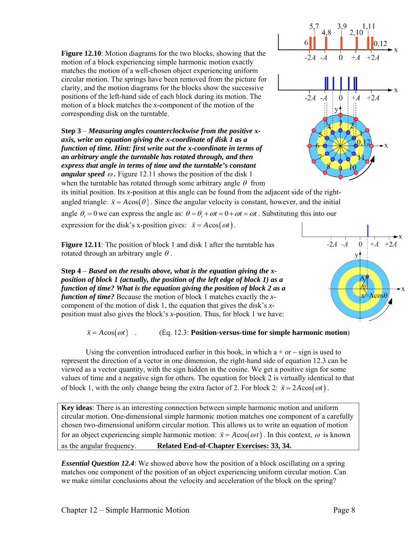
Figure 12.10: Motion diagrams for the two blocks, showing that the motion of a block experiencing simple harmonic motion exactly matches the motion of a well-chosen object experiencing uniform circular motion. The springs have been removed from the picture for clarity, and the motion diagrams for the blocks show the successive positions of the left-hand side of each block during its motion. The motion of a block matches the x-component of the motion of the corresponding disk on the turntable.

Step 3 – Measuring angles counterclockwise from the positive x-axis, write an equation giving the x-coordinate of disk 1 as a function of time. Hint: first write out the x-coordinate in terms of an arbitrary angle the turntable has rotated through, and then express that angle in terms of time and the turntable’s constant angular speed ω . Figure 12.11 shows the position of the disk 1 when the turntable has rotated through some arbitrary angle θ from its initial position. Its x-position at this angle can be found from the adjacent side of the right-angled triangle: ( )cosx A θ=v . Since the angular velocity is constant, however, and the initial angle 0iθ = we can express the angle as: 0i t t tθ θ ω ω ω= + = + = . Substituting this into our expression for the disk’s x-position gives: ( )cosx A tω=v .

Figure 12.11: The position of block 1 and disk 1 after the turntable has rotated through an arbitrary angle θ .

Step 4 – Based on the results above, what is the equation giving the x-position of block 1 (actually, the position of the left edge of block 1) as a function of time? What is the equation giving the position of block 2 as a function of time? Because the motion of block 1 matches exactly the x-component of the motion of disk 1, the equation that gives the disk’s x-position must also gives the block’s x-position. Thus, for block 1 we have:

( )cosx A tω=v . (Eq. 12.3: Position-versus-time for simple harmonic motion) Using the convention introduced earlier in this book, in which a + or – sign is used to

represent the direction of a vector in one dimension, the right-hand side of equation 12.3 can be viewed as a vector quantity, with the sign hidden in the cosine. We get a positive sign for some values of time and a negative sign for others. The equation for block 2 is virtually identical to that of block 1, with the only change being the extra factor of 2. For block 2: ( )2 cosx A tω=v .

Key ideas: There is an interesting connection between simple harmonic motion and uniform circular motion. One-dimensional simple harmonic motion matches one component of a carefully chosen two-dimensional uniform circular motion. This allows us to write an equation of motion for an object experiencing simple harmonic motion: ( )cosx A tω=v . In this context, ω is known as the angular frequency. Related End-of-Chapter Exercises: 33, 34.

Essential Question 12.4: We showed above how the position of a block oscillating on a spring matches one component of the position of an object experiencing uniform circular motion. Can we make similar conclusions about the velocity and acceleration of the block on the spring?


Answer to Essential Question 12.4: Absolutely. All aspects of the motion of the oscillating block match one component of the motion of the object experiencing uniform circular motion. If the position of the block is given by ( )cosx A tω=v , then its velocity and acceleration are given by:

( ) ( ), 1 1 sin sinx disk blockv v v t A tω ω ω= = − = −v v and ( ) ( )2

2, 1 1 cos cosx disk block

va a t A tA

ω ω ω= = − = −v v .

Here v represents the constant speed of disk 1 as it moves in uniform circular motion.

12-5 Hallmarks of Simple Harmonic Motion Simple harmonic motion (often referred to as SHM) is a special case of oscillatory

motion. An object oscillating in one dimension on an ideal spring is a prime example of SHM. The characteristics of simple harmonic motion include:

• A force (and therefore an acceleration) that is opposite in direction, and proportional to, the displacement of the system from equilibrium. Such a force, that acts to restore the system to equilibrium, is known as a restoring force.

• No loss of mechanical energy. • An angular frequency ω that depends on properties of the system. • Position, velocity, and acceleration given by Equations 12.3 – 12.5:

( )cosx A tω=v . (Equation 12.3: Position in simple harmonic motion)

( ) ( )max sin sinv v t A tω ω ω= − = −v . (Equation 12.4: Velocity in SHM)

( ) ( ) ( )2

2max cos cos cosva a t t A t

Aω ω ω ω= − = − = −v . (Eq. 12.5: Acceleration in SHM)

The above equations apply if the object is released from rest from x A= +v at t = 0. Starting the block with different initial conditions requires a modification of the equations.

Combining Equations 12.3 and 12.5, in any simple harmonic motion system we see that

the acceleration is opposite in direction, and proportional to, the displacement: 2a xω= −v v . (Equation 12.6: Connecting acceleration and displacement in SHM)

In general, the angular frequency (ω ), frequency (f), and period (T) are connected by:

22 fTπω π= = . (Eq. 12.7: Relating angular frequency, frequency, and period)

What determines the angular frequency ω in a particular situation? Let’s return to the

free-body diagram of a block on a spring, shown in Figure 12.12.

Figure 12.12: The free-body diagram of a block connected to a spring of spring constant k. The block is displaced to the right of the equilibrium point by a distance x.

Applying Newton’s Second Law horizontally, xF ma∑ =

v v , we get: k x ma− =v v . Re-arranging gives ( / )a k m x= −v v . Comparing this result to the general SHM Equation

12.6 tells us that, for a mass on an ideal spring, 2 /k mω = , or: km

ω = . (Equation 12.8: Angular frequency for a mass on a spring).

This is a typical result, that the angular frequency is given by the square root of a parameter related to the restoring force (or torque, in rotational motion) divided by the inertia.


EXAMPLE 12.5 – Plotting graphs of position, velocity, and acceleration versus time Once again, let’s attach a block to a spring and release the block from rest from a position

x A= +v (relative to 0x =v , which is the equilibrium position). The block oscillates back and forth with a period of T = 4.00 s.

(a) Plot graphs of the block’s position, velocity, and acceleration as a function of time over two complete oscillations.

(b) Compare the position graph to the velocity graph. (c) How does the acceleration graph compare to the position graph?

SOLUTION (a) We can make use of Equations 12.3 – 12.5 to

plot the graphs. Before doing so, we can solve for the angular velocity ω , using:

2 2 rad 1.57 rad / s4.00sT

π πω = = = .

Also, it makes it easier to plot the graphs if we remember that, if the block is released from rest, it returns to its starting point after one period; after half a period it comes instantaneously to rest on the far side of equilibrium; and at times of T/4 and 3T/4 it is passing through equilibrium at its maximum speed. Determining when each graph passes through zero, when it reaches its largest positive and negative values, and then connecting these points with sinusoidally oscillating graphs, gives the results shown in Figure 12.13.

Figure 12.13: Graphs of the position, velocity, and acceleration, as a function of time, of the block in Example 12.5 for two complete oscillations of the block.

(b) Comparing the position and velocity graphs

in Figure 12.13, we can see that the block’s speed is maximum when the block’s displacement from equilibrium is zero. Conversely, the block’s speed is zero when the magnitude of the block’s displacement from equilibrium is maximized. These observations are consistent with what is taking place with the energy. The kinetic energy is proportional to the speed squared and the elastic potential energy is proportional to the square of the magnitude of the displacement from equilibrium. Kinetic energy is maximum when the elastic potential energy is zero, and vice versa.

(c) Comparing the position and acceleration graphs, we see that one is the opposite of the

other, in the sense that when the position is positive the acceleration is negative, and vice versa. This is expected because one of the hallmarks of simple harmonic motion is that 2a xω= −v v . Related End-of-Chapter Exercises: 22, 31, 37.

Essential Question 12.5: Return to the situation described in Example 12.5, but now increase the angular frequency by a factor of 2. We can accomplish this by either changing only the spring constant or by changing only the mass. Can we tell which one was changed by looking at the resulting graphs of position, velocity, and/or acceleration as a function of time? Assume that the block is released from rest from the same point it was in Example 12.5, and that the equilibrium position remains the same.


Answer to Essential Question 12.5: We cannot tell. Any one of the three graphs can be used to determine that the angular frequency has changed, because they all involve ω , but none of the graphs can tell us whether we adjusted the spring constant or the mass.

12-6 Examples Involving Simple Harmonic Motion

EXAMPLE 12.6A – Energy graphs Take a 0.500-kg block and attach it to a spring. We would like the block to undergo

oscillations that have a period (the time for one complete oscillation) of 4.00 seconds. (a) What should the spring constant be? (b) We’ll release the block from rest from a distance A from the equilibrium point so that

the block has a speed of 4.00 m/s when it passes through equilibrium. Over two complete oscillations, plot the system’s elastic potential energy, kinetic energy, and total mechanical energy as a function of time.

SOLUTION (a) Let’s first apply Equation 12.7, 2 /Tω π= , to find the angular frequency. This gives:

2 rad rad / s4.00s 2.00π πω = = .

Using Equation 12.7, km

ω = , we get: ( )22 2 20.500

rad kg / s 1.23N / m4.00

k mπ

ω= = = ,

where we treated the factor of radians as being dimensionless.

Figure 12.14: A diagram of the block and spring, showing the initial situation and the situation as the block passes through equilibrium.

(b) A diagram of the situation is shown in Figure

12.14. Let’s solve for the maximum kinetic energy, which equals the mechanical energy:

( )( )22max max

1 1 0.500kg 4.00m / s 4.00J2 2

K mv= = = .

The maximum potential energy is also 4.00 J, because the energy oscillates between potential and kinetic, and the total mechanical energy is conserved.

Using Equation 12.4, ( )max sinv v tω= −v , we can write the kinetic energy as a function of

time as ( ) ( )2 2 2 2max

1 1 sin 4.00J sin2 2 2.00s

K mv mv t tπω⎛ ⎞

= = = ⎜ ⎟⎝ ⎠

.

Because the block takes 4.00 s to complete one oscillation, at t = 0 and t = 4.00 s it is instantaneously at rest at the starting point. At t = 2.00 s (halfway through the cycle) the block is instantaneously at rest on the far side of equilibrium. At each of these times the kinetic energy is 0 and the elastic potential energy is 4.00 J. Conversely, at t = 1.00 s and 3.00 s it passes through equilibrium, where the elastic potential energy is zero and the kinetic energy is its maximum value of 4.00 J. Graphs of the various energies as a function of time are shown in Figure 12.15. Note that, at all times, the sum of the kinetic and potential energies is 4.00 J.



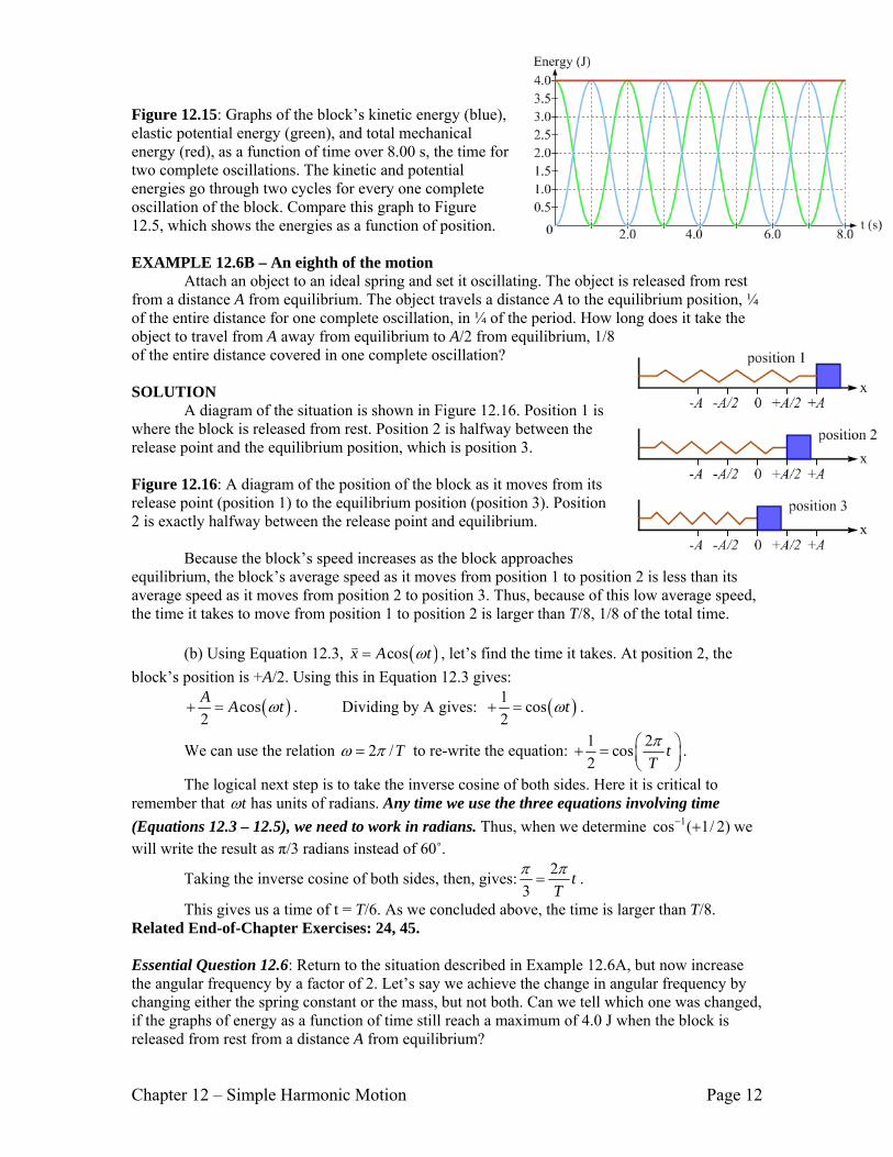
Figure 12.15: Graphs of the block’s kinetic energy (blue), elastic potential energy (green), and total mechanical energy (red), as a function of time over 8.00 s, the time for two complete oscillations. The kinetic and potential energies go through two cycles for every one complete oscillation of the block. Compare this graph to Figure 12.5, which shows the energies as a function of position.

EXAMPLE 12.6B – An eighth of the motion

Attach an object to an ideal spring and set it oscillating. The object is released from rest from a distance A from equilibrium. The object travels a distance A to the equilibrium position, ¼ of the entire distance for one complete oscillation, in ¼ of the period. How long does it take the object to travel from A away from equilibrium to A/2 from equilibrium, 1/8 of the entire distance covered in one complete oscillation?

SOLUTION

A diagram of the situation is shown in Figure 12.16. Position 1 is where the block is released from rest. Position 2 is halfway between the release point and the equilibrium position, which is position 3.

Figure 12.16: A diagram of the position of the block as it moves from its release point (position 1) to the equilibrium position (position 3). Position 2 is exactly halfway between the release point and equilibrium.

Because the block’s speed increases as the block approaches

equilibrium, the block’s average speed as it moves from position 1 to position 2 is less than its average speed as it moves from position 2 to position 3. Thus, because of this low average speed, the time it takes to move from position 1 to position 2 is larger than T/8, 1/8 of the total time.

(b) Using Equation 12.3, ( )cosx A tω=v , let’s find the time it takes. At position 2, the

block’s position is +A/2. Using this in Equation 12.3 gives:

( )cos2A A tω+ = . Dividing by A gives: ( )1 cos

2tω+ = .

We can use the relation 2 /Tω π= to re-write the equation: 1 2cos2

tTπ⎛ ⎞+ = ⎜ ⎟

⎝ ⎠.

The logical next step is to take the inverse cosine of both sides. Here it is critical to remember that tω has units of radians. Any time we use the three equations involving time (Equations 12.3 – 12.5), we need to work in radians. Thus, when we determine 1cos ( 1/ 2)− + we will write the result as π/3 radians instead of 60˚.

Taking the inverse cosine of both sides, then, gives: 23

tT

π π= .

This gives us a time of t = T/6. As we concluded above, the time is larger than T/8. Related End-of-Chapter Exercises: 24, 45.

Essential Question 12.6: Return to the situation described in Example 12.6A, but now increase the angular frequency by a factor of 2. Let’s say we achieve the change in angular frequency by changing either the spring constant or the mass, but not both. Can we tell which one was changed, if the graphs of energy as a function of time still reach a maximum of 4.0 J when the block is released from rest from a distance A from equilibrium?


Answer to Essential Question 12.6: Consider Equation 12.8, /k mω = . We can double the angular frequency by increasing the spring constant by a factor of 4, or by decreasing the mass by a factor of 4. Because the object is released from rest, the initial energy is all elastic potential energy, given by 20.5iU k A= . We have not changed A, so if the total energy stayed the same we must not have changed the spring constant k. Thus we must have changed the mass.

12-7 The Simple Pendulum Another classic simple harmonic motion system is the simple pendulum, which is an

object with mass that swings back and forth on a string of negligible mass. EXAMPLE 12.7 – Pendulum speed limit

A ball of mass m is fastened to a string with a length L. Initially the ball hangs vertically down from the string in its equilibrium position. The ball is then displaced so the string makes an angle of θ with the vertical, and then released from rest.

(a) What is the height of the ball above the equilibrium position when it is released? (b) What is the speed of the ball when it passes through equilibrium?

SOLUTION (a) Consider the geometry of the situation, shown in Figure 12.17.

Figure 12.17: A diagram showing the point from which the ball is released and the equilibrium position.

The key to finding the height of the ball is to consider the right-angled triangle in Figure 12.17. The vertical side of the triangle measures cosL θ . Because the string measures L, the height of the ball above equilibrium is ( )cos 1 cosh L L Lθ θ= − = − .

(b) Let’s apply energy conservation, starting as usual with: i i nc f fK U W K U+ + = + .

The initial point is the release point, while the final point is the equilibrium position. 0iK = , because the ball is released from rest from the initial point. 0ncW = , because there is no work being done by non-conservative forces.

We can define the ball’s gravitational potential energy to be zero at the equilibrium point, giving 0fU = .

The equation thus reduces to i fU K= , which gives: 212 fmgh mv= .

The mass cancels out, so the speed does not depend on the mass. Solving for the speed: 2 2 (1 cos )fv gh gL θ= = − .

Note that we have seen this 2fv gh= result before, such as in cases in which an object falls straight down from rest, or when water leaks out a hole in a container.

Related End-of-Chapter Exercises: 19, 51. EXPLORATION 12.7 – Torques on the pendulum

A simple pendulum consists of a ball of mass m that hangs down vertically from a string. The ball is displaced by an angle θ from equilibrium and released from rest.


Step 1 – Draw a free-body diagram for the ball immediately after it is released. The free-body diagram is drawn in Figure 12.18). There is a downward force of gravity, and a force of tension directed away from the ball along the string. Using a coordinate system aligned with the string, we can split the force of gravity into components, one component opposite to the tension and the other component giving an acceleration toward the equilibrium position (see Figure 12.18(b)).

Figure 12.18: Figure (a) shows the free-body diagram, with a force of tension and a force of gravity acting on the ball. Figure (b) shows the force of gravity in components, using a coordinate system in which one axis is parallel to the string.

Step 2 – Apply Newton’s Second Law for Rotation to find a relationship between the angular acceleration of the ball and the ball’s angular displacement (measured from the vertical). Take torques about the axis perpendicular to the page passing through the upper end of the string. There is no torque about this axis from the tension or from the component of the force of gravity parallel to the string. The only torque comes from the component of the force of gravity that acts perpendicular to the string. Applying sinr Fτ φ= , where r = L, sinF mg θ= , and 90φ = ° , the torque has a magnitude of sinLmgτ θ= . Taking counterclockwise to be positive, the torque is negative. Applying Newton’s Second Law for Rotation, Iτ α∑ = vv , we get: sinLmg Iθ α− = v .

The rotational inertia of the ball is 2I mL= , giving: 2sinLmg mLθ α− = v . Canceling the mass (thus, the mass does not matter) and a factor of L gives:

singL

α θ= −v . (Equation 12.9: Angular acceleration of a simple pendulum)

Step 3 – Use the small-angle approximation, sinθ θ≈ , to find an expression for the angular frequency of the pendulum. We can say that sinθ θ≈ if θ is given in radians, and the angle is less than about 10˚(about 1/6 radians). Using the small-angle approximation in Equation 12.9:

gL

α θ= −vv . (Equation 12.10: For a simple pendulum at small angles)

The general simple harmonic relationship, 2a xω= −v v , can be transformed to an analogous general equation for rotational motion, 2α ω θ= −

vv . Equation 12.10 fits this form, so:

gL

ω = . (Eq. 12.11: Angular frequency for a simple pendulum at small angles)

For a pendulum, gravity provides the restoring force, so it makes sense that the angular frequency is larger if g is larger. Conversely, increasing L means the pendulum has farther to travel to reach equilibrium, reducing the angular frequency.

Key ideas: For small-angle oscillations, the motion of a simple pendulum is simple harmonic. Large-angle oscillations are not simple harmonic because the restoring torque is not proportional to the angular displacement. Related End-of-Chapter Exercises: 54, 55. Essential Question 12.7: Compare the free-body diagram of a ball of mass m, hanging at rest from a string of length L, to that of the same system oscillating as a pendulum, when the ball passes through equilibrium. Make note of any differences between the two free-body diagrams.


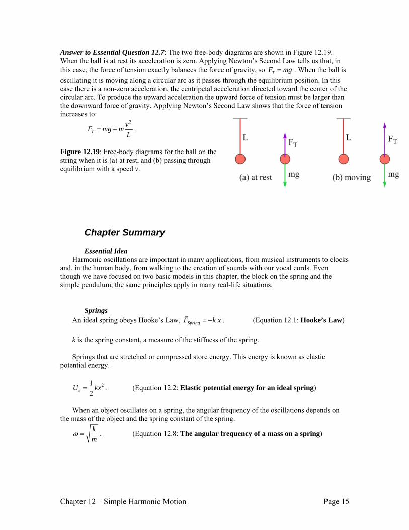
Answer to Essential Question 12.7: The two free-body diagrams are shown in Figure 12.19. When the ball is at rest its acceleration is zero. Applying Newton’s Second Law tells us that, in this case, the force of tension exactly balances the force of gravity, so TF mg= . When the ball is oscillating it is moving along a circular arc as it passes through the equilibrium position. In this case there is a non-zero acceleration, the centripetal acceleration directed toward the center of the circular arc. To produce the upward acceleration the upward force of tension must be larger than the downward force of gravity. Applying Newton’s Second Law shows that the force of tension increases to:

2

TvF mg mL

= + .

Figure 12.19: Free-body diagrams for the ball on the string when it is (a) at rest, and (b) passing through equilibrium with a speed v.

Chapter Summary

Essential Idea

Harmonic oscillations are important in many applications, from musical instruments to clocks and, in the human body, from walking to the creation of sounds with our vocal cords. Even though we have focused on two basic models in this chapter, the block on the spring and the simple pendulum, the same principles apply in many real-life situations.

Springs An ideal spring obeys Hooke’s Law, SpringF k x= −

v v . (Equation 12.1: Hooke’s Law) k is the spring constant, a measure of the stiffness of the spring. Springs that are stretched or compressed store energy. This energy is known as elastic

potential energy.

212eU kx= . (Equation 12.2: Elastic potential energy for an ideal spring)

When an object oscillates on a spring, the angular frequency of the oscillations depends on

the mass of the object and the spring constant of the spring. km

ω = . (Equation 12.8: The angular frequency of a mass on a spring)


Simple Harmonic Motion and Energy Conservation Energy conservation is a useful tool for analyzing oscillating systems. When springs are

involved we use elastic potential energy, an idea introduced in this chapter. To analyze a pendulum in terms of energy conservation nothing new whatsoever is needed.

Hallmarks of Simple Harmonic Motion The main features of a system that undergoes simple harmonic motion include:

• No loss of mechanical energy. • A restoring force or torque that is proportional to, and opposite in direction to, the

displacement of the system from equilibrium.

In this situation the acceleration of the system is related to its position by: 2a xω= −v v , (Eq. 12.6: The connection between acceleration and displacement) where the angular frequency ω is generally given by the square root of some elastic property

of the system (such as the spring constant) divided by an inertial property (such as the mass).

Time and Simple Harmonic Motion When we are interested in how a simple harmonic oscillator evolves over time the following

equations are extremely useful. These were derived by looking at the connection between simple harmonic motion and one component of the motion of an object experiencing uniform circular motion.

( )cosx A tω=v . (Equation 12.3: Position in simple harmonic motion)

( )sinv A tω ω= −v . (Equation 12.4: Velocity in simple harmonic motion)

( )2 cosa A tω ω= −v . (Eq. 12.5: Acceleration in simple harmonic motion)

Equations 12.3 – 12.5 apply when the object is released from rest at t = 0 from a distance A from equilibrium.

In general, the angular frequency (ω ), frequency (f), and period (T) are connected by:

22 fTπω π= = . (Eq. 12.7: Relating angular frequency, frequency, and period)

The Simple Pendulum A simple pendulum, consisting of an object on the end of a string, is another good example of

an oscillating system. As long as the amplitude of the oscillations is small (less than about 10˚) and mechanical energy is conserved then the motion is simple harmonic. For larger angles the motion diverges from simple harmonic because the restoring torque is not directly proportional to the angular displacement.

gL

ω = . (Equation 12.11: Angular frequency of a simple pendulum)

Documents

Chapter 12 – Simple Harmonic Motionphysics.bu.edu/~duffy/ns544_summer2009_notes02/NS544_online1.pdf · Chapter 12 – Simple Harmonic Motion Page 3 Answer to Essential Question