Embed Size (px)
Citation preview

Chapter 14 – Cluster Analysis
© Galit Shmueli and Peter Bruce 2010
Data Mining for Business Intelligence
Shmueli, Patel & Bruce

Clustering: The Main Idea
Goal: Form groups (clusters) of similar records
Used for segmenting markets into groups of similar
customers
Example: Claritas segmented US neighborhoods
based on demographics & income: “Furs & station
wagons,” “Money & Brains”, …

Other Applications
Periodic table of the elements
Classification of species

Classification of Mammals

Other Applications
Grouping securities in portfolios
Grouping firms for structural analysis of economy
Army uniform sizes

Example: Public Utilities
Goal: find clusters of similar utilities
Data: 22 firms, 8 variables
Fixed-charge covering ratio
Rate of return on capital
Cost per kilowatt capacity
Annual load factor
Growth in peak demand
Sales
% nuclear
Fuel costs per kwh

Company Fixed_charge RoR Cost Load D Demand Sales Nuclear Fuel_Cost
Arizona 1.06 9.2 151 54.4 1.6 9077 0 0.628
Boston 0.89 10.3 202 57.9 2.2 5088 25.3 1.555
Central 1.43 15.4 113 53 3.4 9212 0 1.058
Commonwealth 1.02 11.2 168 56 0.3 6423 34.3 0.7
Con Ed NY 1.49 8.8 192 51.2 1 3300 15.6 2.044
Florida 1.32 13.5 111 60 -2.2 11127 22.5 1.241
Hawaiian 1.22 12.2 175 67.6 2.2 7642 0 1.652
Idaho 1.1 9.2 245 57 3.3 13082 0 0.309
Kentucky 1.34 13 168 60.4 7.2 8406 0 0.862
Madison 1.12 12.4 197 53 2.7 6455 39.2 0.623
Nevada 0.75 7.5 173 51.5 6.5 17441 0 0.768
New England 1.13 10.9 178 62 3.7 6154 0 1.897
Northern 1.15 12.7 199 53.7 6.4 7179 50.2 0.527
Oklahoma 1.09 12 96 49.8 1.4 9673 0 0.588
Pacific 0.96 7.6 164 62.2 -0.1 6468 0.9 1.4
Puget 1.16 9.9 252 56 9.2 15991 0 0.62
San Diego 0.76 6.4 136 61.9 9 5714 8.3 1.92
Southern 1.05 12.6 150 56.7 2.7 10140 0 1.108
Texas 1.16 11.7 104 54 -2.1 13507 0 0.636
Wisconsin 1.2 11.8 148 59.9 3.5 7287 41.1 0.702
United 1.04 8.6 204 61 3.5 6650 0 2.116
Virginia 1.07 9.3 174 54.3 5.9 10093 26.6 1.306
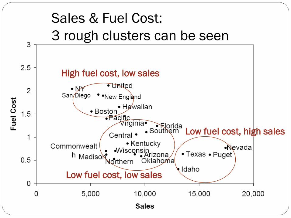
Low fuel cost, low sales
Sales & Fuel Cost:
3 rough clusters can be seen
High fuel cost, low sales
Low fuel cost, high sales

Clustering is Ambiguous
How many clusters?
Four Clusters Two Clusters
Six Clusters

Extension to More Than 2 Dimensions
In prior example, clustering was done by eye
Multiple dimensions require formal algorithm with
A distance measure
A way to use the distance measure in forming clusters
We will consider two algorithms: hierarchical and non-
hierarchical

Hierarchical Clustering
p4
p1p3
p2
p4
p1 p3
p2
p4p1 p2 p3
p4p1 p2 p3
Traditional Hierarchical Clustering
Non-traditional Hierarchical Clustering Non-traditional Dendrogram
Traditional Dendrogram

Partitional Clustering
Original Points A Partitional Clustering

Hierarchical Clustering

A Dendrogram shows the cluster hierarchy

Hierarchical Methods
Agglomerative Methods
Begin with n-clusters (each record its own cluster)
Keep joining records into clusters until one cluster is
left (the entire data set)
Most popular
Divisive Methods
Start with one all-inclusive cluster
Repeatedly divide into smaller clusters


Measuring Distance
Between records
Between clusters

Measuring Distance Between Records

Distance Between Two Records
Euclidean Distance is most popular:

Normalizing
Problem: Raw distance measures are highly influenced
by scale of measurements
Solution: normalize (standardize) the data first
Subtract mean, divide by std. deviation
Also called z-scores

Example: Normalization
For 22 utilities:
Avg. sales = 8,914
Std. dev. = 3,550
Normalized score for Arizona sales:
(9,077-8,914)/3,550 = 0.046

For Categorical Data: Similarity
Similarity metrics based on this table:
Matching coef. = (a+d)/p
Jaquard’s coef. = d/(b+c+d)
Use in cases where a matching “1” is much greater
evidence of similarity than matching “0” (e.g. “owns
Corvette”)
0 1
0 a b
1 c d
To measure the distance between records in terms
of two 0/1 variables, create table with counts:

Other Distance Measures
Correlation-based similarity
Statistical distance (Mahalanobis)
Manhattan distance (absolute differences)
Maximum coordinate distance
Gower’s similarity (for mixed variable types:
continuous & categorical)

Measuring Distance Between Clusters
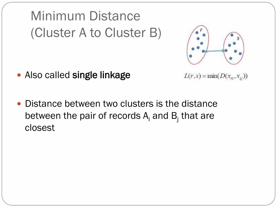
Minimum Distance
(Cluster A to Cluster B)
Also called single linkage
Distance between two clusters is the distance
between the pair of records Ai and Bj that are
closest

Maximum Distance
(Cluster A to Cluster B)
Also called complete linkage
Distance between two clusters is the distance
between the pair of records Ai and Bj that are
farthest from each other

Average Distance
Also called average linkage
Distance between two clusters is the average of all
possible pair-wise distances

Centroid Distance
Distance between two clusters is the distance between
the two cluster centroids.
Centroid is the vector of variable averages for all
records in a cluster

The Hierarchical Clustering Steps (Using
Agglomerative Method)
1. Start with n clusters (each record is its own cluster)
2. Merge two closest records into one cluster
3. At each successive step, the two clusters closest to
each other are merged
Dendrogram, from bottom up, illustrates the process

Records 12 & 21 are closest & form first cluster

Reading the Dendrogram
See process of clustering: Lines connected lower down
are merged earlier
10 and 13 will be merged next, after 12 & 21
Determining number of clusters: For a given “distance
between clusters”, a horizontal line intersects the
clusters that are that far apart, to create clusters
E.g., at distance of 4.6 (red line in next slide), data can be
reduced to 2 clusters -- The smaller of the two is circled
At distance of 3.6 (green line) data can be reduced to 6
clusters, including the circled cluster


Validating Clusters
Interpretation
Goal: obtain meaningful and useful clusters
Caveats:
(1) Random chance can often produce apparent clusters
(2) Different cluster methods produce different results
Solutions:
Obtain summary statistics
Also review clusters in terms of variables not used in
clustering
Label the cluster (e.g. clustering of financial firms in
2008 might yield label like “midsize, sub-prime loser”)

Desirable Cluster Features
Stability – are clusters and cluster assignments
sensitive to slight changes in inputs? Are cluster
assignments in partition B similar to partition A?
Separation – check ratio of between-cluster variation
to within-cluster variation (higher is better)

Nonhierarchical Clustering:
K-Means Clustering

K-Means Clustering Algorithm
1. Choose # of clusters desired, k
2. Start with k random centroids (a partition into k
random clusters)
3. repeat until (new assignment increases within-
cluster dispersion)
1. assign each record to the closest cluster (min
distance between record and centroid)
2. Update centroids, repeat step 3

Minimizing total intra-cluster variance
K-means Algorithm:
Choosing k and Initial Partitioning
Choose k based on the how results will be used
e.g., “How many market segments do we want?”
Also experiment with slightly different k’s
Initial partition into clusters can be random, or based
on domain knowledge
If random partition, repeat the process with different random
partitions

K-means Clustering – Details
Initial centroids are often chosen randomly.
Clusters produced vary from one run to another.
The centroid is (typically) the mean of the points in the cluster.
‘Closeness’ is measured by Euclidean distance, cosine similarity, correlation, etc.
K-means will converge for common similarity measures mentioned above.
Most of the convergence happens in the first few iterations.
Often the stopping condition is changed to ‘Until relatively few points change clusters’
Complexity is O( n * K * I * d )
n = number of points, K = number of clusters, I = number of iterations, d = number of attributes

Two different K-means Clusterings
-2 -1.5 -1 -0.5 0 0.5 1 1.5 2
0
0.5
1
1.5
2
2.5
3
x
y
-2 -1.5 -1 -0.5 0 0.5 1 1.5 2
0
0.5
1
1.5
2
2.5
3
x
y
Sub-optimal Clustering
-2 -1.5 -1 -0.5 0 0.5 1 1.5 2
0
0.5
1
1.5
2
2.5
3
x
y
Optimal Clustering
Original Points

Importance of Choosing Initial Centroids
-2 -1.5 -1 -0.5 0 0.5 1 1.5 2
0
0.5
1
1.5
2
2.5
3
x
y
Iteration 1
-2 -1.5 -1 -0.5 0 0.5 1 1.5 2
0
0.5
1
1.5
2
2.5
3
x
y
Iteration 2
-2 -1.5 -1 -0.5 0 0.5 1 1.5 2
0
0.5
1
1.5
2
2.5
3
x
y
Iteration 3
-2 -1.5 -1 -0.5 0 0.5 1 1.5 2
0
0.5
1
1.5
2
2.5
3
x
y
Iteration 4
-2 -1.5 -1 -0.5 0 0.5 1 1.5 2
0
0.5
1
1.5
2
2.5
3
x
y
Iteration 5
-2 -1.5 -1 -0.5 0 0.5 1 1.5 2
0
0.5
1
1.5
2
2.5
3
x
y
Iteration 6

Evaluating K-means Clusters Most common measure is Sum of Squared Error (SSE)
For each point, the error is the distance to the nearest cluster
To get SSE, we square these errors and sum them.
x is a data point in cluster Ci and mi is the representative point for cluster Ci
can show that mi corresponds to the center (mean) of the cluster
Given two clusters, we can choose the one with the smallest error
One easy way to reduce SSE is to increase K, the number of clusters
A good clustering with smaller K can have a lower SSE than a poor clustering with higher K
K
i Cx
i
i
xmdistSSE1
2 ),(

Importance of Choosing Initial Centroids …
-2 -1.5 -1 -0.5 0 0.5 1 1.5 2
0
0.5
1
1.5
2
2.5
3
x
y
Iteration 1
-2 -1.5 -1 -0.5 0 0.5 1 1.5 2
0
0.5
1
1.5
2
2.5
3
x
y
Iteration 2
-2 -1.5 -1 -0.5 0 0.5 1 1.5 2
0
0.5
1
1.5
2
2.5
3
x
y
Iteration 3
-2 -1.5 -1 -0.5 0 0.5 1 1.5 2
0
0.5
1
1.5
2
2.5
3
x
y
Iteration 4
-2 -1.5 -1 -0.5 0 0.5 1 1.5 2
0
0.5
1
1.5
2
2.5
3
x
y
Iteration 5

Importance of Choosing Initial Centroids …
-2 -1.5 -1 -0.5 0 0.5 1 1.5 2
0
0.5
1
1.5
2
2.5
3
x
y
Iteration 1
-2 -1.5 -1 -0.5 0 0.5 1 1.5 2
0
0.5
1
1.5
2
2.5
3
x
y
Iteration 2
-2 -1.5 -1 -0.5 0 0.5 1 1.5 2
0
0.5
1
1.5
2
2.5
3
x
y
Iteration 3
-2 -1.5 -1 -0.5 0 0.5 1 1.5 2
0
0.5
1
1.5
2
2.5
3
x
y
Iteration 4
-2 -1.5 -1 -0.5 0 0.5 1 1.5 2
0
0.5
1
1.5
2
2.5
3
xy
Iteration 5
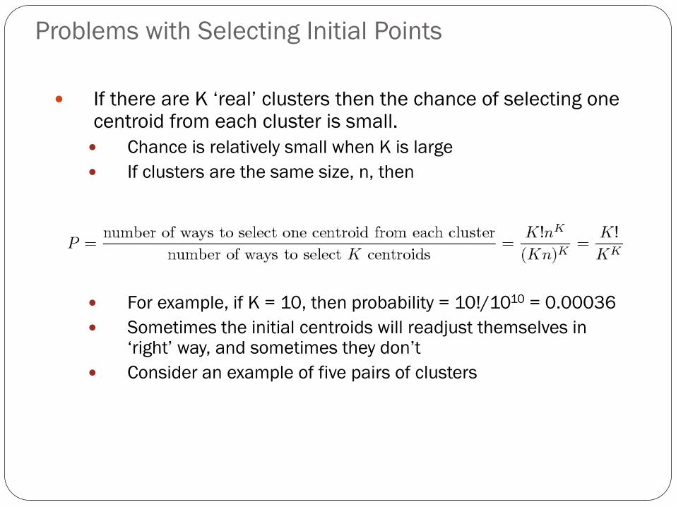
Problems with Selecting Initial Points
If there are K ‘real’ clusters then the chance of selecting one centroid from each cluster is small.
Chance is relatively small when K is large
If clusters are the same size, n, then
For example, if K = 10, then probability = 10!/1010 = 0.00036
Sometimes the initial centroids will readjust themselves in ‘right’ way, and sometimes they don’t
Consider an example of five pairs of clusters

10 Clusters Example
0 5 10 15 20
-6
-4
-2
0
2
4
6
8
x
yIteration 1
0 5 10 15 20
-6
-4
-2
0
2
4
6
8
x
yIteration 2
0 5 10 15 20
-6
-4
-2
0
2
4
6
8
x
yIteration 3
0 5 10 15 20
-6
-4
-2
0
2
4
6
8
x
yIteration 4
Starting with two initial centroids in one cluster of each pair of clusters

10 Clusters Example
0 5 10 15 20
-6
-4
-2
0
2
4
6
8
x
y
Iteration 1
0 5 10 15 20
-6
-4
-2
0
2
4
6
8
x
y
Iteration 2
0 5 10 15 20
-6
-4
-2
0
2
4
6
8
x
y
Iteration 3
0 5 10 15 20
-6
-4
-2
0
2
4
6
8
x
y
Iteration 4
Starting with two initial centroids in one cluster of each pair of clusters

10 Clusters Example
Starting with some pairs of clusters having three initial centroids, while other
have only one.
0 5 10 15 20
-6
-4
-2
0
2
4
6
8
x
y
Iteration 1
0 5 10 15 20
-6
-4
-2
0
2
4
6
8
x
y
Iteration 2
0 5 10 15 20
-6
-4
-2
0
2
4
6
8
x
y
Iteration 3
0 5 10 15 20
-6
-4
-2
0
2
4
6
8
x
y
Iteration 4

10 Clusters Example
Starting with some pairs of clusters having three initial centroids, while other
have only one.
0 5 10 15 20
-6
-4
-2
0
2
4
6
8
x
yIteration 1
0 5 10 15 20
-6
-4
-2
0
2
4
6
8
x
y
Iteration 2
0 5 10 15 20
-6
-4
-2
0
2
4
6
8
x
y
Iteration 3
0 5 10 15 20
-6
-4
-2
0
2
4
6
8
x
y
Iteration 4

Solutions to Initial Centroids
Problem
Multiple runs
Helps, but probability is not on your side
Sample and use hierarchical clustering to determine initial centroids
Select more than k initial centroids and then select among these initial centroids
Select most widely separated
Postprocessing
Bisecting K-means
Not as susceptible to initialization issues

Updating Centers Incrementally
In the basic K-means algorithm, centroids are
updated after all points are assigned to a centroid
An alternative is to update the centroids after each
assignment (incremental approach)
Each assignment updates zero or two centroids
More expensive
Introduces an order dependency
Never get an empty cluster
Can use “weights” to change the impact
A simpler version of Self Organizing Map neural
network

Pre-processing and Post-processing
Pre-processing
Normalize the data
Eliminate outliers
Post-processing
Eliminate small clusters that may represent outliers
Split ‘loose’ clusters, i.e., clusters with relatively high
SSE
Merge clusters that are ‘close’ and that have relatively
low SSE
Can use these steps during the clustering process
ISODATA

XLMiner Output: Cluster Centroids
We chose k = 3
4 of the 8 variables are shown
Cluster Fixed_charge RoR Cost Load_factor
Cluster-1 0.89 10.3 202 57.9
Cluster-2 1.43 15.4 113 53
Cluster-3 1.06 9.2 151 54.4

Distance Between Clusters
Clusters 1 and 2 are relatively well-separated
from each other, while cluster 3 not as much
Distance
between
cluster
Cluster-1 Cluster-2 Cluster-3
Cluster-1 0 5.03216253 3.16901457
Cluster-2 5.03216253 0 3.76581196
Cluster-3 3.16901457 3.76581196 0
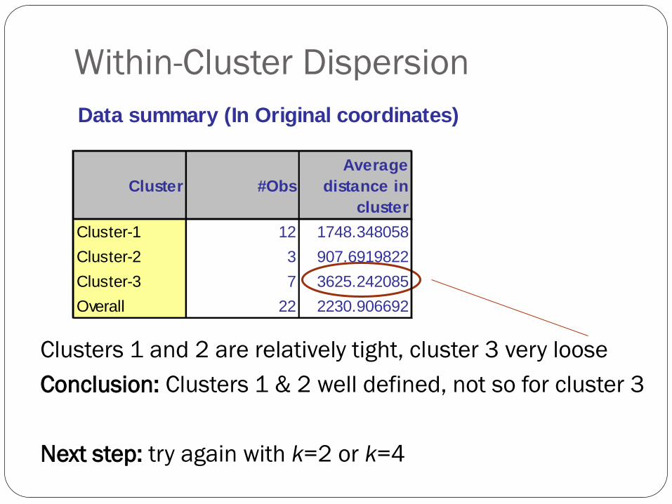
Within-Cluster Dispersion
Clusters 1 and 2 are relatively tight, cluster 3 very loose
Conclusion: Clusters 1 & 2 well defined, not so for cluster 3
Next step: try again with k=2 or k=4
Data summary (In Original coordinates)
Cluster #Obs
Average
distance in
cluster
Cluster-1 12 1748.348058
Cluster-2 3 907.6919822
Cluster-3 7 3625.242085
Overall 22 2230.906692

• a(i) 데이터 i 와 같은 클러스터에 속한 다른
데이터들과의 평균 “거리”
• 작을수록?
• i 는 잘 “맞는” 클러스터에 소속됨
Silhouette 실루엣 Peter J. Rousseeuw 1986

• b(i) 데이터 i 와 다른 클러스터에 속한 데이터들
과의 평균 “거리” 가 최소인 “이웃” 클러스터의
데이터들 간 평균 거리
• i 가 현재 클러스터 다음으로 “잘 맞는” 클러스터 (즉, “이웃”)
• b(i) 가 크다면?
• “이웃” 클러스터가 실제 별로 이웃이 아님
Silhouette 실루엣 Peter J. Rousseeuw 1986

• b(i) >> a(i) 라면 ?
• 제대로 클러스터 됨
• b(i) << a(i) 라면 ?
• i 는 이웃 클러스터로 가는 게 나음
Silhouette 실루엣 Peter J. Rousseeuw 1986

• b(i) >> a(i) 라면 ?
• 제대로 클러스터 됨, s => 1
• b(i) << a(i) 라면 ?
• i 는 이웃 클러스터로 가는 게 나음, s => -1
Silhouette 실루엣 Peter J. Rousseeuw 1986
실루엣 plot
각 클러스터 별로,
데이터 들을 s(i) 큰 순서대로 정렬하여 수평선으로
표시

아래 데이터를 k-medoid 로 군집화


Density based Clustering

Dunn Index (Dunn, 1974)
ratio between the minimal inter-cluster distance to
maximal intra-cluster distance.
d(i,j) : the distance between clusters i and j
d '(k) : the intra-cluster distance of cluster k
clusters with high Dunn index are more
desirable

Applications
Data Exploration and Understanding
Data Compression: codebook
Market Segmentation
Multiple Regression / Classification models
Characterization of Normality in Novelty Detection
Summary
Cluster analysis is an exploratory tool. Useful only
when it produces meaningful clusters
Hierarchical clustering gives visual representation of
different levels of clustering
On other hand, due to non-iterative nature, it can be
unstable, can vary highly depending on settings, and is
computationally expensive

Summary
Non-hierarchical is computationally cheap and more
stable; requires user to set k
Can use both methods
Be wary of chance results; data may not have
definitive “real” clusters


![WELCOME [theor.jinr.ru]theor.jinr.ru/~diastp/dm15/talks/Opening-DM2015.pdf · Startup Topics from the field “Structure of Matter” (2004 - 2006): 1. Hot Points in Astrophysics](https://img.pdfslide.us/doc/110x75/5fb9a6a60f397933452d4b76/welcome-theorjinrrutheorjinrrudiastpdm15talksopening-startup-topics.jpg)