Waves

191

Chapter 11 Waves

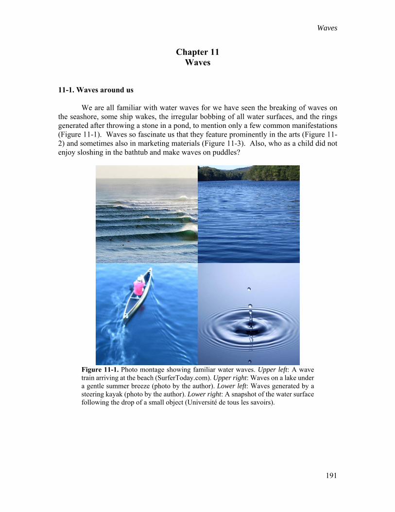
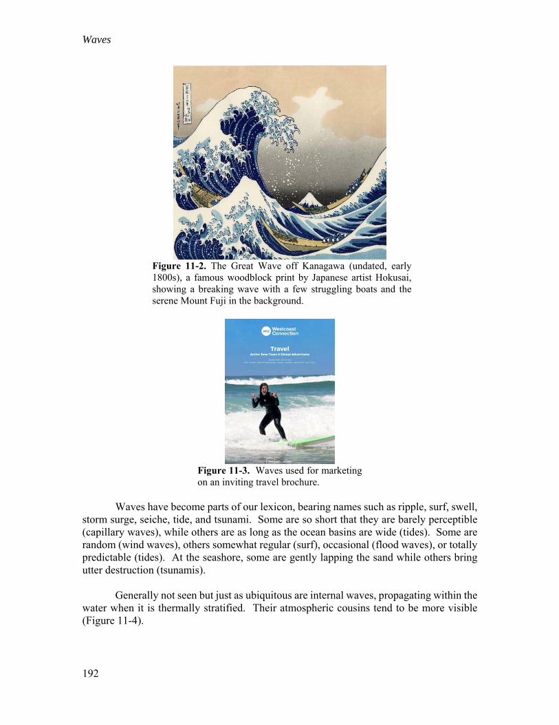
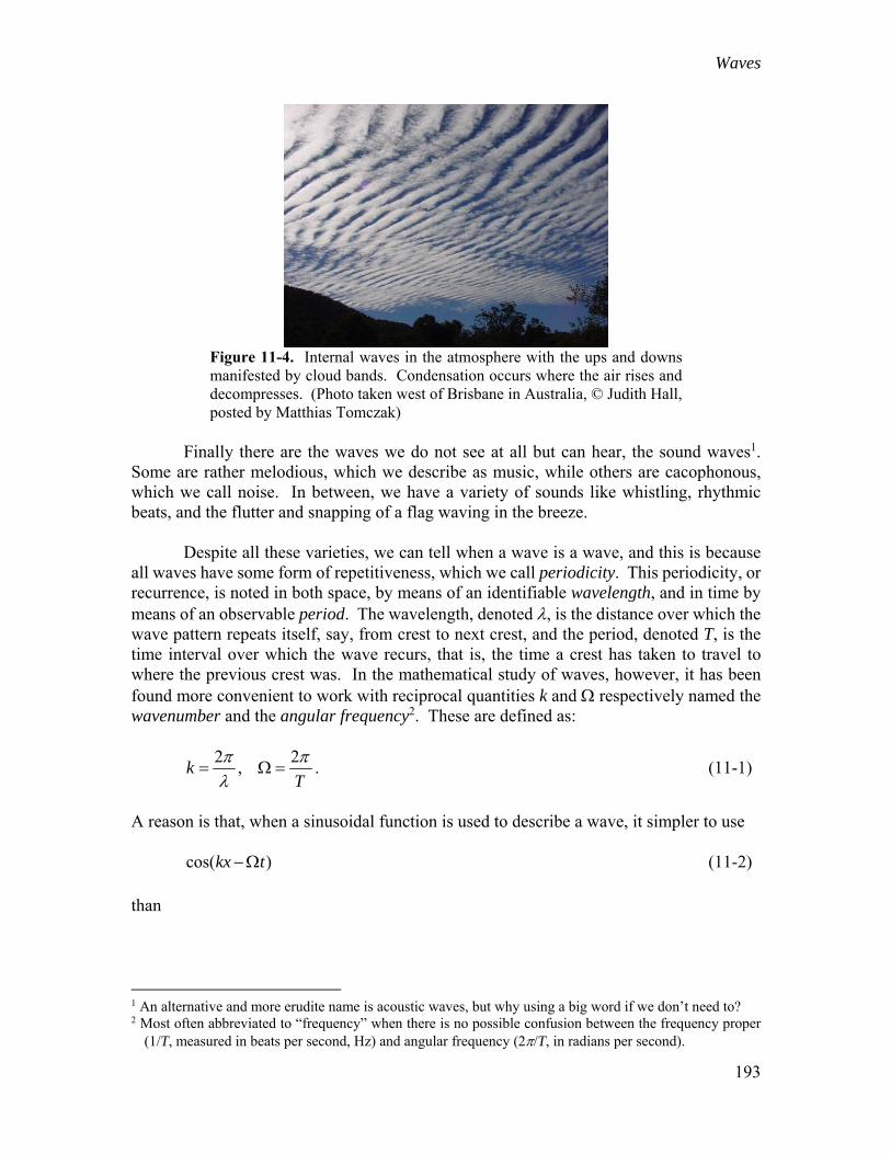
11-1. Waves around us We are all familiar with water waves for we have seen the breaking of waves on the seashore, some ship wakes, the irregular bobbing of all water surfaces, and the rings generated after throwing a stone in a pond, to mention only a few common manifestations (Figure 11-1). Waves so fascinate us that they feature prominently in the arts (Figure 11-2) and sometimes also in marketing materials (Figure 11-3). Also, who as a child did not enjoy sloshing in the bathtub and make waves on puddles?

Figure 11-1. Photo montage showing familiar water waves. Upper left: A wave train arriving at the beach (SurferToday.com). Upper right: Waves on a lake under a gentle summer breeze (photo by the author). Lower left: Waves generated by a steering kayak (photo by the author). Lower right: A snapshot of the water surface following the drop of a small object (Université de tous les savoirs).

Waves

192

Figure 11-2. The Great Wave off Kanagawa (undated, early 1800s), a famous woodblock print by Japanese artist Hokusai, showing a breaking wave with a few struggling boats and the serene Mount Fuji in the background.

Figure 11-3. Waves used for marketing on an inviting travel brochure.

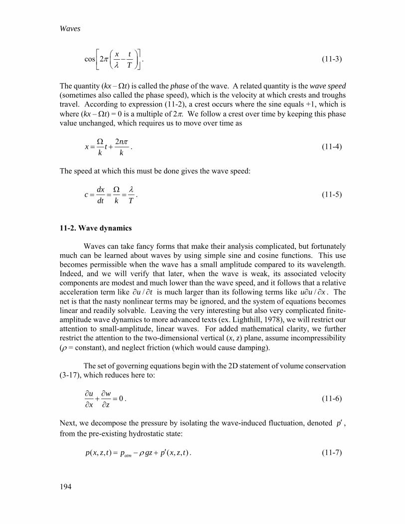
Waves have become parts of our lexicon, bearing names such as ripple, surf, swell, storm surge, seiche, tide, and tsunami. Some are so short that they are barely perceptible (capillary waves), while others are as long as the ocean basins are wide (tides). Some are random (wind waves), others somewhat regular (surf), occasional (flood waves), or totally predictable (tides). At the seashore, some are gently lapping the sand while others bring utter destruction (tsunamis). Generally not seen but just as ubiquitous are internal waves, propagating within the water when it is thermally stratified. Their atmospheric cousins tend to be more visible (Figure 11-4).

Waves

193

Figure 11-4. Internal waves in the atmosphere with the ups and downs manifested by cloud bands. Condensation occurs where the air rises and decompresses. (Photo taken west of Brisbane in Australia, © Judith Hall, posted by Matthias Tomczak)

Finally there are the waves we do not see at all but can hear, the sound waves1. Some are rather melodious, which we describe as music, while others are cacophonous, which we call noise. In between, we have a variety of sounds like whistling, rhythmic beats, and the flutter and snapping of a flag waving in the breeze. Despite all these varieties, we can tell when a wave is a wave, and this is because all waves have some form of repetitiveness, which we call periodicity. This periodicity, or recurrence, is noted in both space, by means of an identifiable wavelength, and in time by means of an observable period. The wavelength, denoted , is the distance over which the wave pattern repeats itself, say, from crest to next crest, and the period, denoted T, is the time interval over which the wave recurs, that is, the time a crest has taken to travel to where the previous crest was. In the mathematical study of waves, however, it has been found more convenient to work with reciprocal quantities k and respectively named the wavenumber and the angular frequency2. These are defined as:

2 2

,kT

. (11-1)

A reason is that, when a sinusoidal function is used to describe a wave, it simpler to use cos( )kx t (11-2) than

1 An alternative and more erudite name is acoustic waves, but why using a big word if we don’t need to? 2 Most often abbreviated to “frequency” when there is no possible confusion between the frequency proper

(1/T, measured in beats per second, Hz) and angular frequency (2/T, in radians per second).

Waves

194

cos 2x t

T

. (11-3)

The quantity (kx – t) is called the phase of the wave. A related quantity is the wave speed (sometimes also called the phase speed), which is the velocity at which crests and troughs travel. According to expression (11-2), a crest occurs where the sine equals +1, which is where (kx – t) = 0 is a multiple of 2. We follow a crest over time by keeping this phase value unchanged, which requires us to move over time as

2n

x tk k

. (11-4)

The speed at which this must be done gives the wave speed:

dx

cdt k T

. (11-5)

11-2. Wave dynamics Waves can take fancy forms that make their analysis complicated, but fortunately much can be learned about waves by using simple sine and cosine functions. This use becomes permissible when the wave has a small amplitude compared to its wavelength. Indeed, and we will verify that later, when the wave is weak, its associated velocity components are modest and much lower than the wave speed, and it follows that a relative acceleration term like /u t is much larger than its following terms like /u u x . The net is that the nasty nonlinear terms may be ignored, and the system of equations becomes linear and readily solvable. Leaving the very interesting but also very complicated finite-amplitude wave dynamics to more advanced texts (ex. Lighthill, 1978), we will restrict our attention to small-amplitude, linear waves. For added mathematical clarity, we further restrict the attention to the two-dimensional vertical (x, z) plane, assume incompressibility ( = constant), and neglect friction (which would cause damping). The set of governing equations begin with the 2D statement of volume conservation (3-17), which reduces here to:

0u w

x z

. (11-6)

Next, we decompose the pressure by isolating the wave-induced fluctuation, denoted p , from the pre-existing hydrostatic state: ( , , ) ( , , )atmp x z t p gz p x z t . (11-7)

Waves

195

With this decomposition and the aforementioned neglect of friction and of the nonlinear acceleration terms, the two momentum equations are very simply:

1u p

t x

(11-8a)

1w p

t z

, (11-8b)

each expressing a balance between relative acceleration and pressure force. The solution to this set of equations is readily expressed in terms of sine and cosine functions: ( , , ) ( ) cos ( )p x z t P z k x ct (11-9a)

1( , , ) ( ) cos ( )u x z t P z k x ct

c (11-9b)

1( , , ) sin ( )

dPw x z t k x ct

kc dz , (11-9c)

after use of (11-8a,b) to reduce the problem to a single unknown function P(z), which is the vertical variation of the wave-induced contribution to pressure. Note that p and u are

in phase while w is out of phase with these two. The vertical displacement of fluid particles can be inferred from the expression for the vertical velocity w:

2 2

1( , , ) cos ( )

dPw x z t k x ct

t k c dz

. (11-10)

The remaining unknown function P(z) is determined after substitution of the preceding expressions in the volume conservation equation (11-6), which yields:

2

22

d Pk P

dz . (11-11)

The general solution is the sum of two exponentials: ( ) kz kzP z P e P e

. (11-12)

The presence of two constants of integration (P+ and P–) necessitates the stating of two boundary conditions, one on top and one below. Different choices for these boundary conditions lead to different types of waves. Before delving into this, however, it is instructive to verify that our assumption of small-amplitude waves indeed corresponds to velocity components that are small

Waves

196

compared to the wave speed and allows us to neglect the nonlinear acceleration terms. The wave amplitude is said to be small when vertical displacements are small compared to the wavelength, i.e., . According to (11-10), this means that the pressure function P(z)

must be such that 2( ) 2P z c . (11-13)

for which we have also used (11-1) to go from wavelength to wavenumber and (11-12) to express the size of the dP/dz. Signs can be conveniently ignored in a size-only analysis. Using this inequality in expressions (11-9b,c), we see that the velocity components must each be capped by: and 2u w c . (11-14)

So, indeed, small amplitude implies velocities that are small compared to the wave speed. As acceleration terms are concerned, the ratio of nonlinear acceleration to relative acceleration are all of the type:

( / )

2/

u u x u

u t c

. (11-15)

Two other properties of this solution are worth noting. First, expressions (11-9b,c) imply / / 0u z w x , which means that the waves under consideration have no vorticity. The flow is said to be irrotational. Second, these same expressions together with relation (11-11) lead to 2 2 0u w , which means that internal viscous friction can only have an effect on the solution through a boundary condition. This is not to say that all surface water waves are free from viscous damping, only small-amplitude waves over deep water. 11-2-a. Deep-water waves By deep water, we mean a case where the effect of the wave on top (near z = 0) is not felt at the bottom. Mathematically this is tantamount to stating that the bottom situated at z = – H is so far below the top that the first exponential in (11-12) is negligible:

1 12

kHe kH H

. (11-16)

In practice, H > is sufficient. Needless to say, the other exponential in (11-12) “blows up” as the bottom is approached, which means that we need discard this term. In other words, the bottom boundary conditions becomes P– = 0.

Waves

197

At the top, we consider that the water has a free surface, with averaged level z = 0. As the water surface makes a wave, it develops curvature with which goes a certain surface tension according to (5-1) and adds or subtracts water weight. The net effect is that at the averaged water level, there is a wave-induced pressure contribution equal to:

0 0capillary gravityp p p gR

, (11-17)

in which R is the radius of curvature of the surface, positive where downward (adding pressure – see Figure 5-1) and the subscript 0 indicates that the function is taken at the surface, which is nearly z = 0 by virtue of the small-amplitude assumption. The geometric relation giving the surface curvature 1/R from its vertical displacement 0 is:

20

220

3/2 22

0

1

1

xR x

x

, (11-18)

with the simplification being justified by the small-amplitude approximation once again. With this, the upper boundary condition to be imposed is:

2

00 02

p gx

. (11-19)

Substitution of the periodic functions and a little algebra leads to the following requirement:

2 2cos ( ) cos ( )

k gP k x ct P k x ct

c kc

.

For this to be satisfied in the presence of a wave [P+(0) ≠ 0] at all positions x and times t, we must have:

2 2

1k g

c kc

,

which specifies a relationship between wave speed c and wavenumber k and therefore wavelength3:

3 The negative root is allowed, too, but it only corresponds to the same wave traveling in the negative x-

direction instead of the positive x-direction.

Waves

198

2

2

k g gc

k

. (11-20)

This tells us that all waves with the same wavelength will travel at the same speed, and that waves of different wavelengths will travel at different speeds. An initial group of waves with different wavelengths will therefore unravel itself with the faster waves outrunning the slower waves. This is called wave dispersion, and formula (11-20) is called the dispersion relation. The presence of two terms under the square root goes back to the fact we invoked two effects at the surface, surface tension effect and gravity, giving rise to the terms with and g, respectively. The question arises: Which is biggest? The answer depends of course on the wavelength. So, let us first seek the particular value of the wavelength that makes the two terms equal to each other and denote it with a star subscript. A little algebra gives us:

* 2g

. (11-21)

For water at ambient temperature, this value of about 1.7 cm (two thirds of an inch), a rather small value. Around this value, we can discern two asymptotic regimes: a short wavelength regime with * and a long wavelength regime with * .

The case of short wavelength leads to an approximate wave speed:

2k

c

(11-22)

that corresponds to waves purely driven by surface tension, called capillary waves. The shorter these waves are, the faster they travel. Since * is a requirement for these

waves, they can only be rather short. Figure 11-5 shows two examples. At sea and on lakes and ponds, capillary waves are generated by the wind. They act as the “hook” with which the water surface takes energy from the wind. That energy is then transferred through nonlinear wave-wave interactions (not studied here) into longer waves.

Waves

199

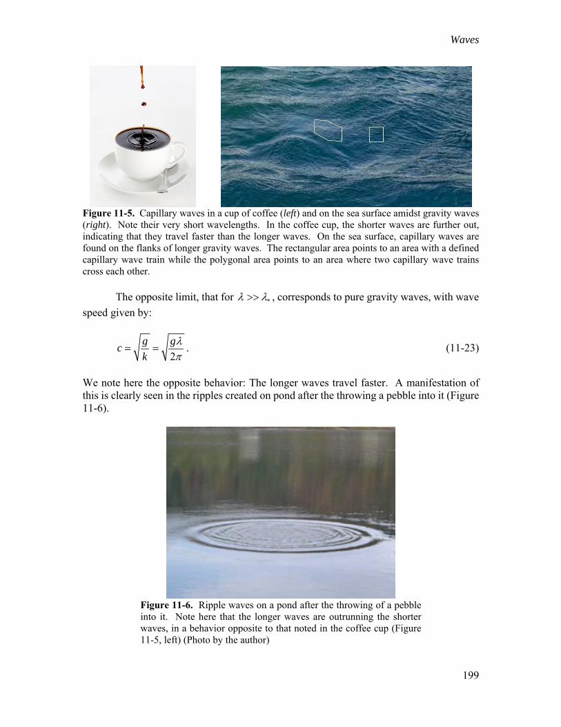
Figure 11-5. Capillary waves in a cup of coffee (left) and on the sea surface amidst gravity waves (right). Note their very short wavelengths. In the coffee cup, the shorter waves are further out, indicating that they travel faster than the longer waves. On the sea surface, capillary waves are found on the flanks of longer gravity waves. The rectangular area points to an area with a defined capillary wave train while the polygonal area points to an area where two capillary wave trains cross each other. The opposite limit, that for * , corresponds to pure gravity waves, with wave

speed given by:

2

g gc

k

. (11-23)

We note here the opposite behavior: The longer waves travel faster. A manifestation of this is clearly seen in the ripples created on pond after the throwing a pebble into it (Figure 11-6).

Figure 11-6. Ripple waves on a pond after the throwing of a pebble into it. Note here that the longer waves are outrunning the shorter waves, in a behavior opposite to that noted in the coffee cup (Figure 11-5, left) (Photo by the author)

Waves

200

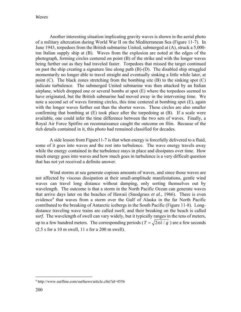
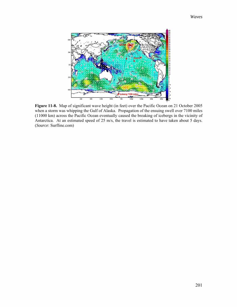
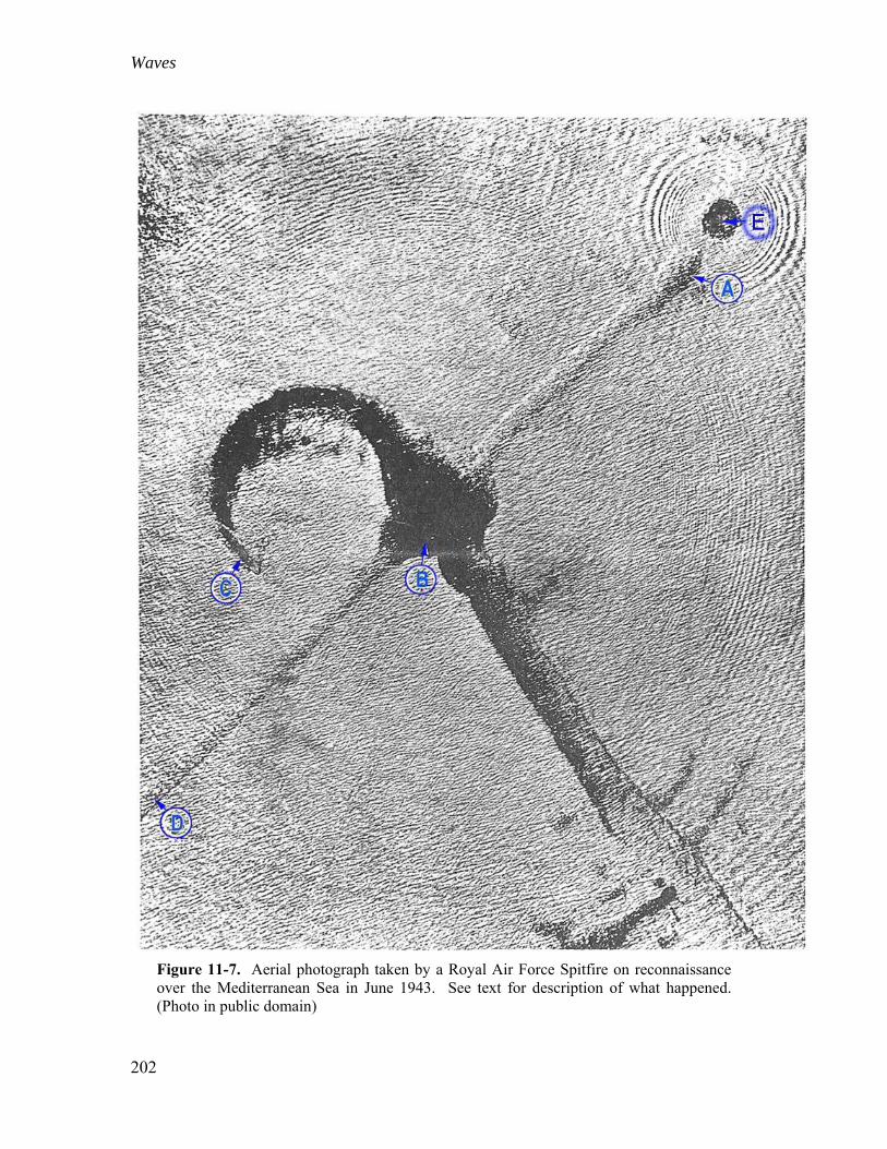
Another interesting situation implicating gravity waves is shown in the aerial photo of a military altercation during World War II on the Mediterranean Sea (Figure 11-7). In June 1943, torpedoes from the British submarine United, submerged at (A), struck a 5,000-ton Italian supply ship at (B). Waves from the explosion are noted at the edges of the photograph, forming circles centered on point (B) of the strike and with the longer waves being further out as they had traveled faster. Torpedoes that missed the target continued on past the ship creating a signature line along path (B)-(D). The disabled ship struggled momentarily no longer able to travel straight and eventually sinking a little while later, at point (C). The black zones stretching from the bombing site (B) to the sinking spot (C) indicate turbulence. The submerged United submarine was then attacked by an Italian airplane, which dropped one or several bombs at spot (E) where the torpedoes seemed to have originated, but the British submarine had moved away in the intervening time. We note a second set of waves forming circles, this time centered at bombing spot (E), again with the longer waves further out than the shorter waves. These circles are also smaller confirming that bombing at (E) took place after the torpedoing at (B). If a scale were available, one could infer the time difference between the two sets of waves. Finally, a Royal Air Force Spitfire on reconnaissance caught the outcome on film. Because of the rich details contained in it, this photo had remained classified for decades. A side lesson from Figure11-7 is that when energy is forcefully delivered to a fluid, some of it goes into waves and the rest into turbulence. The wave energy travels away while the energy contained in the turbulence stays in place and dissipates over time. How much energy goes into waves and how much goes in turbulence is a very difficult question that has not yet received a definite answer. Wind storms at sea generate copious amounts of waves, and since those waves are not affected by viscous dissipation at their small-amplitude manifestations, gentle wind waves can travel long distance without damping, only sorting themselves out by wavelength. The outcome is that a storm in the North Pacific Ocean can generate waves that arrive days later on the beaches of Hawaii (Snodgrass et al., 1966). There is even evidence4 that waves from a storm over the Gulf of Alaska in the far North Pacific contributed to the breaking of Antarctic icebergs in the South Pacific (Figure 11-8). Long-distance traveling wave trains are called swell, and their breaking on the beach is called surf. The wavelength of swell can vary widely, but it typically ranges in the tens of meters,

up to a few hundred meters. The corresponding periods ( 2 /T g ) are a few seconds

(2.5 s for a 10 m swell, 11 s for a 200 m swell).

4 http://www.surfline.com/surfnews/article.cfm?id=4556

Waves

201

Figure 11-8. Map of significant wave height (in feet) over the Pacific Ocean on 21 October 2005 when a storm was whipping the Gulf of Alaska. Propagation of the ensuing swell over 7100 miles (11000 km) across the Pacific Ocean eventually caused the breaking of icebergs in the vicinity of Antarctica. At an estimated speed of 25 m/s, the travel is estimated to have taken about 5 days. (Source: Surfline.com)

Waves

202

Figure 11-7. Aerial photograph taken by a Royal Air Force Spitfire on reconnaissance over the Mediterranean Sea in June 1943. See text for description of what happened. (Photo in public domain)

Waves

203

11-2-b. Shallow-water waves We now consider the case of a shallow body of water, with flat bottom at z = – H. As the vertical velocity must be zero on a horizontal impermeable bottom, we impose w = 0 there. So, we now need to retain both exponentials in solution (11-12), but in order to continue making our live easy, we restrict the attention to very long waves, namely waves with wavelengths much longer than the water depth: >> H. This means that the product

2 /kz kH H is very small. In practice, it is sufficient to take > 20H.

For small |kz|, the exponentials may be replaced by their first few terms of their Taylor expansion, and we have:

2 21( ) ( ) ( ) ( )

2P z P P P P kz P P k z . (11-24)

The vertical velocity given by (11-9c) becomes:

1( , , ) ( ) ( ) sin ( )w x z t P P P P kz k x ct

c ,

Since it must vanish at the bottom z = –H, we need to have

01 1

P PP

kH kH

. (11-25)

where the quantity P0 is defined for convenience and symmetry. With this, the wave-induced pressure and velocity components become at their respective leading order: 0( , , ) 2 cos ( )p x z t P k x ct (11-26a)

0

2( , , ) cos ( )u x z t P k x ct

c (11-26b)

0

2 ( )( , , ) sin ( )

k H zw x z t P k x ct

c

. (11-26c)

From the vertical velocity follows the vertical displacement:

02

2( )( , , ) cos ( )

H zx z t P k x ct

c

. (11-27)

We now apply the boundary condition at the surface, which is (11-19) without the surface tension effect which is negligible for long waves. The outcome is:

Waves

204

0 022 cos ( ) 2 cos ( )

gHP k x ct P k x ct

c ,

which may be satisfied at all places and time only if5

c gH . (11-28)

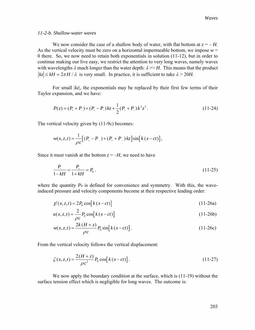
We note that these waves all have the same speed, regardless of wavelength. They are said to be non-dispersive, and it means that a group of shallow-water waves does not become distorted over time. Because they are forced by the distant gravitational pull of the moon and sun, tides occupy the entire ocean basins in which they exist. This gives them wavelengths of thousands of kilometers, while the ocean basins are only a few kilometers deep. Thus, although the oceans may appear deep to us when we sail across one with a ship, tides are actually shallow-water waves. Had we not performed a Taylor extension on the solution for P(z), we would have obtained the speed of surface gravity waves of any wavelength, tying the deep-water and shallow water results (11-23) and (11-28) into a single dispersion relation. The algebra is not particularly interesting, and we only quote here the end result:

tanh( )g

c kHk

. (11-29)

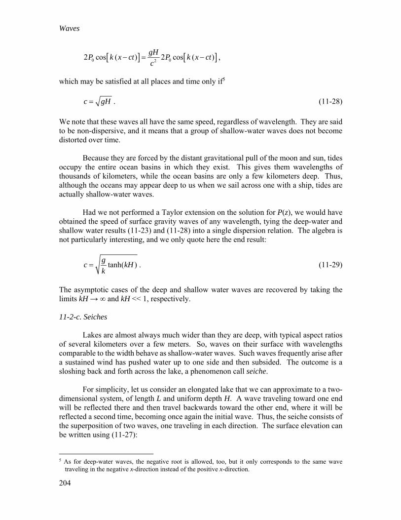
The asymptotic cases of the deep and shallow water waves are recovered by taking the limits kH → ∞ and kH << 1, respectively. 11-2-c. Seiches Lakes are almost always much wider than they are deep, with typical aspect ratios of several kilometers over a few meters. So, waves on their surface with wavelengths comparable to the width behave as shallow-water waves. Such waves frequently arise after a sustained wind has pushed water up to one side and then subsided. The outcome is a sloshing back and forth across the lake, a phenomenon call seiche. For simplicity, let us consider an elongated lake that we can approximate to a two-dimensional system, of length L and uniform depth H. A wave traveling toward one end will be reflected there and then travel backwards toward the other end, where it will be reflected a second time, becoming once again the initial wave. Thus, the seiche consists of the superposition of two waves, one traveling in each direction. The surface elevation can be written using (11-27): 5 As for deep-water waves, the negative root is allowed, too, but it only corresponds to the same wave

traveling in the negative x-direction instead of the positive x-direction.

Waves

205

1 22

2( )( , , ) cos ( ) cos ( )

H zx z t P k x ct P k x ct

c

(11-30)

with the P1-wave traveling at speed c gH in the positive x-direction while the P2-wave

travels backward at the same speed. A possible phase shift was added to the phase of the second wave. Expression (11-26b) provides the associated horizontal velocity:

1 2

2( , , ) cos ( ) cos ( )u x z t P k x ct P k x ct

c

. (11-31)

(The negative sign in front of the P2 amplitude is caused by that wave having a speed –c.) At each end of the lake (x = 0 and x = L), the horizontal velocity must vanish at all times. Enforcing this at x = 0 yields P1 = P2 and = 0. Using this and then enforcing the zero-velocity condition at x = L, we obtain that the expression cos( ) cos( )kL kct kL kct .must be satisfied at all times, and the only way to make this possible is to have sin 0kL . It follows that wavenumbers, and therefore also wavelengths, may only take discrete values:

2 3

, , ,kL L L

and

2 22 , , ,

3L L L

k

(11-32)

The longest possible wavelength, which corresponds to the basic sloshing of water in the lake, called the fundamental mode or 1st mode, is such that the basin contains only have of the wavelength. The situation is depicted in Figure 11-9. The two waves add up to a signal that does not propagate but oscillates in space. This is called a standing wave.

Figure 11-9: The fundamental seiche mode in an elongated basin with flat bottom.

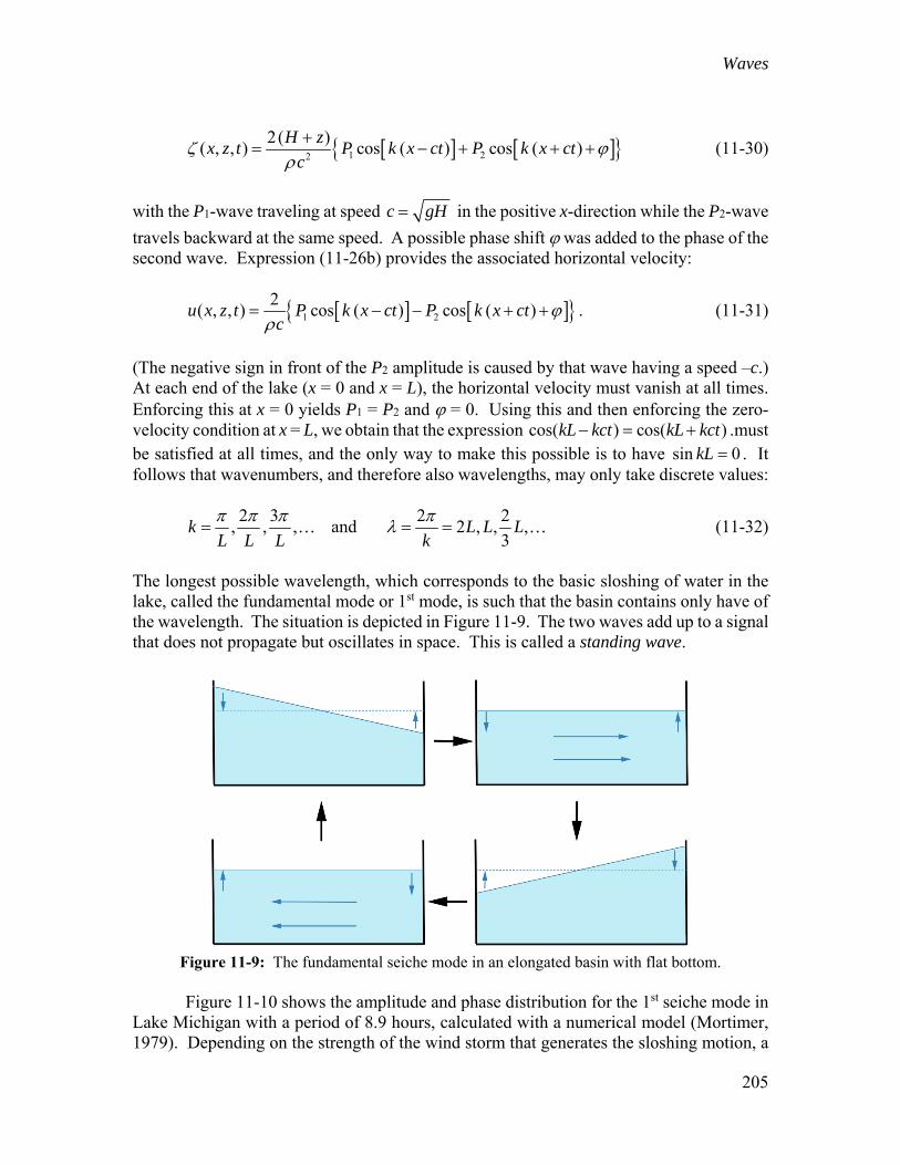
Figure 11-10 shows the amplitude and phase distribution for the 1st seiche mode in Lake Michigan with a period of 8.9 hours, calculated with a numerical model (Mortimer, 1979). Depending on the strength of the wind storm that generates the sloshing motion, a

Waves

206

seiche in Lake Michigan can reach several meters. An occurrence of a 2.44-m seiche killed eight people on a dock in Chicago by surprise on 26 June 1954.

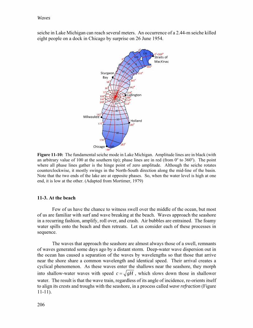
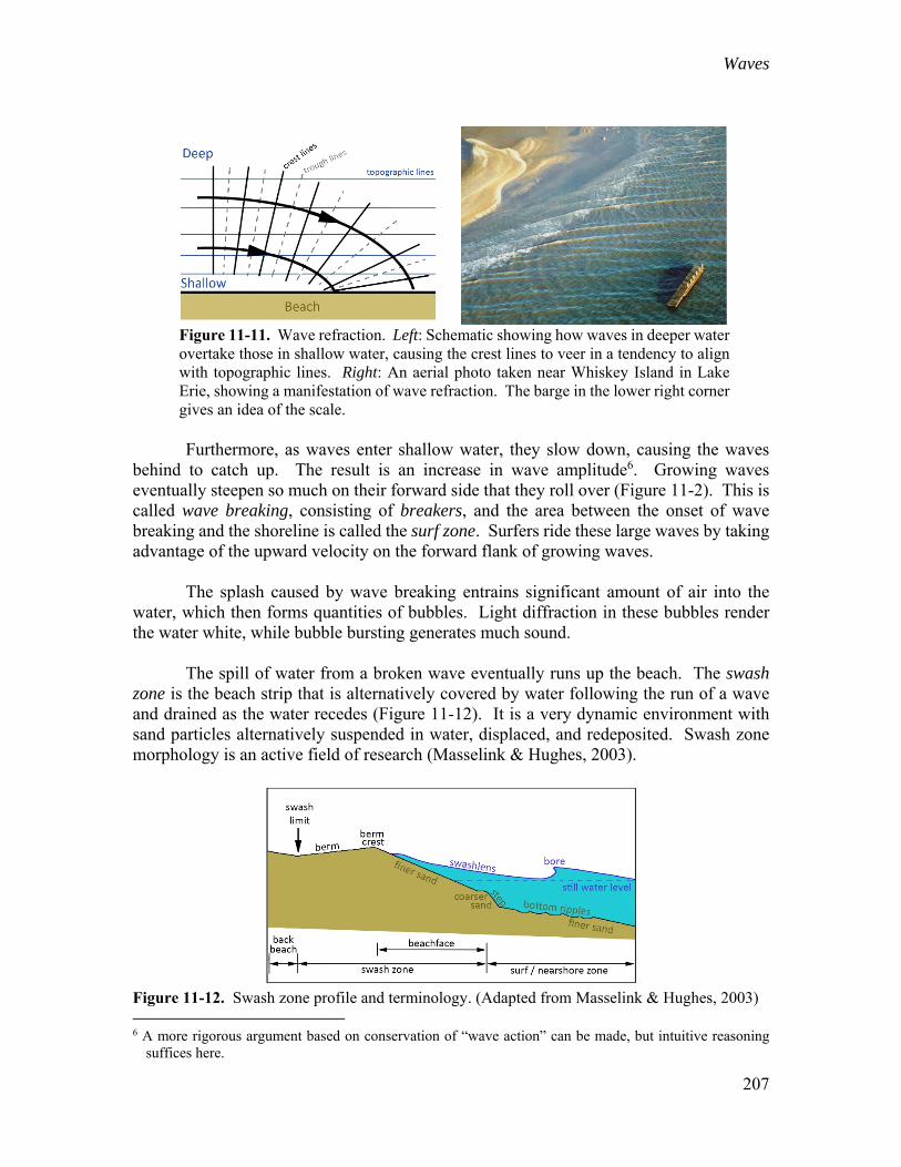
Figure 11-10: The fundamental seiche mode in Lake Michigan. Amplitude lines are in black (with an arbitrary value of 100 at the southern tip); phase lines are in red (from 0o to 360o). The point where all phase lines gather is the hinge point of zero amplitude. Although the seiche rotates counterclockwise, it mostly swings in the North-South direction along the mid-line of the basin. Note that the two ends of the lake are at opposite phases. So, when the water level is high at one end, it is low at the other. (Adapted from Mortimer, 1979) 11-3. At the beach Few of us have the chance to witness swell over the middle of the ocean, but most of us are familiar with surf and wave breaking at the beach. Waves approach the seashore in a recurring fashion, amplify, roll over, and crash. Air bubbles are entrained. The foamy water spills onto the beach and then retreats. Let us consider each of these processes in sequence. The waves that approach the seashore are almost always those of a swell, remnants of waves generated some days ago by a distant storm. Deep-water wave dispersion out in the ocean has caused a separation of the waves by wavelengths so that those that arrive near the shore share a common wavelength and identical speed. Their arrival creates a cyclical phenomenon. As these waves enter the shallows near the seashore, they morph

into shallow-water waves with speed c gH , which slows down those in shallower

water. The result is that the wave train, regardless of its angle of incidence, re-orients itself to align its crests and troughs with the seashore, in a process called wave refraction (Figure 11-11).

Waves

207

Figure 11-11. Wave refraction. Left: Schematic showing how waves in deeper water overtake those in shallow water, causing the crest lines to veer in a tendency to align with topographic lines. Right: An aerial photo taken near Whiskey Island in Lake Erie, showing a manifestation of wave refraction. The barge in the lower right corner gives an idea of the scale.

Furthermore, as waves enter shallow water, they slow down, causing the waves behind to catch up. The result is an increase in wave amplitude6. Growing waves eventually steepen so much on their forward side that they roll over (Figure 11-2). This is called wave breaking, consisting of breakers, and the area between the onset of wave breaking and the shoreline is called the surf zone. Surfers ride these large waves by taking advantage of the upward velocity on the forward flank of growing waves. The splash caused by wave breaking entrains significant amount of air into the water, which then forms quantities of bubbles. Light diffraction in these bubbles render the water white, while bubble bursting generates much sound. The spill of water from a broken wave eventually runs up the beach. The swash zone is the beach strip that is alternatively covered by water following the run of a wave and drained as the water recedes (Figure 11-12). It is a very dynamic environment with sand particles alternatively suspended in water, displaced, and redeposited. Swash zone morphology is an active field of research (Masselink & Hughes, 2003).

Figure 11-12. Swash zone profile and terminology. (Adapted from Masselink & Hughes, 2003) 6 A more rigorous argument based on conservation of “wave action” can be made, but intuitive reasoning

suffices here.

Waves

208

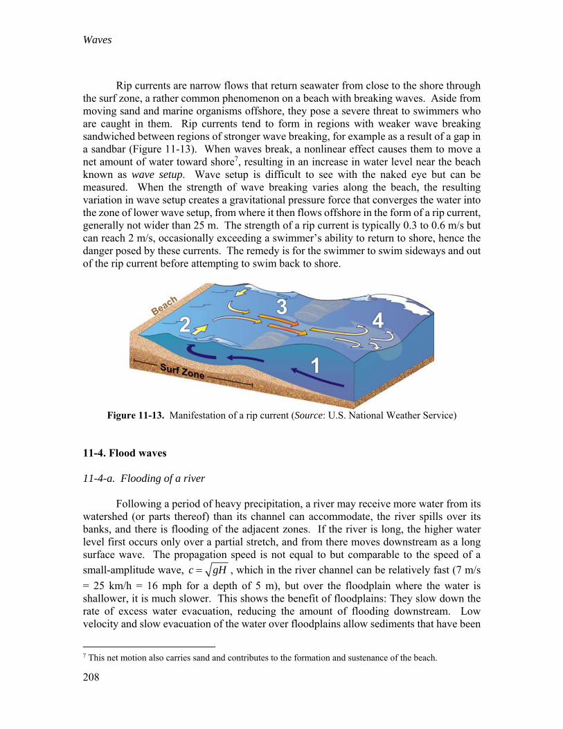
Rip currents are narrow flows that return seawater from close to the shore through the surf zone, a rather common phenomenon on a beach with breaking waves. Aside from moving sand and marine organisms offshore, they pose a severe threat to swimmers who are caught in them. Rip currents tend to form in regions with weaker wave breaking sandwiched between regions of stronger wave breaking, for example as a result of a gap in a sandbar (Figure 11-13). When waves break, a nonlinear effect causes them to move a net amount of water toward shore7, resulting in an increase in water level near the beach known as wave setup. Wave setup is difficult to see with the naked eye but can be measured. When the strength of wave breaking varies along the beach, the resulting variation in wave setup creates a gravitational pressure force that converges the water into the zone of lower wave setup, from where it then flows offshore in the form of a rip current, generally not wider than 25 m. The strength of a rip current is typically 0.3 to 0.6 m/s but can reach 2 m/s, occasionally exceeding a swimmer’s ability to return to shore, hence the danger posed by these currents. The remedy is for the swimmer to swim sideways and out of the rip current before attempting to swim back to shore.

Figure 11-13. Manifestation of a rip current (Source: U.S. National Weather Service)

11-4. Flood waves 11-4-a. Flooding of a river Following a period of heavy precipitation, a river may receive more water from its watershed (or parts thereof) than its channel can accommodate, the river spills over its banks, and there is flooding of the adjacent zones. If the river is long, the higher water level first occurs only over a partial stretch, and from there moves downstream as a long surface wave. The propagation speed is not equal to but comparable to the speed of a

small-amplitude wave, c gH , which in the river channel can be relatively fast (7 m/s

= 25 km/h = 16 mph for a depth of 5 m), but over the floodplain where the water is shallower, it is much slower. This shows the benefit of floodplains: They slow down the rate of excess water evacuation, reducing the amount of flooding downstream. Low velocity and slow evacuation of the water over floodplains allow sediments that have been

7 This net motion also carries sand and contributes to the formation and sustenance of the beach.

Waves

209

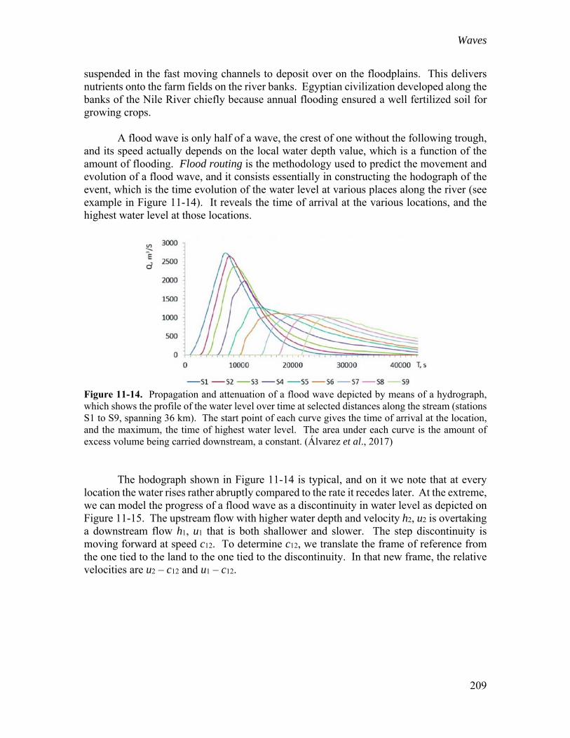
suspended in the fast moving channels to deposit over on the floodplains. This delivers nutrients onto the farm fields on the river banks. Egyptian civilization developed along the banks of the Nile River chiefly because annual flooding ensured a well fertilized soil for growing crops. A flood wave is only half of a wave, the crest of one without the following trough, and its speed actually depends on the local water depth value, which is a function of the amount of flooding. Flood routing is the methodology used to predict the movement and evolution of a flood wave, and it consists essentially in constructing the hodograph of the event, which is the time evolution of the water level at various places along the river (see example in Figure 11-14). It reveals the time of arrival at the various locations, and the highest water level at those locations.

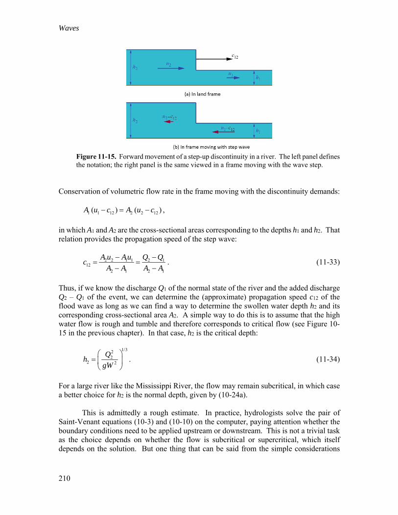
Figure 11-14. Propagation and attenuation of a flood wave depicted by means of a hydrograph, which shows the profile of the water level over time at selected distances along the stream (stations S1 to S9, spanning 36 km). The start point of each curve gives the time of arrival at the location, and the maximum, the time of highest water level. The area under each curve is the amount of excess volume being carried downstream, a constant. (Álvarez et al., 2017) The hodograph shown in Figure 11-14 is typical, and on it we note that at every location the water rises rather abruptly compared to the rate it recedes later. At the extreme, we can model the progress of a flood wave as a discontinuity in water level as depicted on Figure 11-15. The upstream flow with higher water depth and velocity h2, u2 is overtaking a downstream flow h1, u1 that is both shallower and slower. The step discontinuity is moving forward at speed c12. To determine c12, we translate the frame of reference from the one tied to the land to the one tied to the discontinuity. In that new frame, the relative velocities are u2 – c12 and u1 – c12.

Waves

210

Figure 11-15. Forward movement of a step-up discontinuity in a river. The left panel defines the notation; the right panel is the same viewed in a frame moving with the wave step.

Conservation of volumetric flow rate in the frame moving with the discontinuity demands: 1 1 12 2 2 12( ) ( )A u c A u c ,

in which A1 and A2 are the cross-sectional areas corresponding to the depths h1 and h2. That relation provides the propagation speed of the step wave:

2 2 1 1 2 112

2 1 2 1

A u Au Q Qc

A A A A

. (11-33)

Thus, if we know the discharge Q1 of the normal state of the river and the added discharge Q2 – Q1 of the event, we can determine the (approximate) propagation speed c12 of the flood wave as long as we can find a way to determine the swollen water depth h2 and its corresponding cross-sectional area A2. A simple way to do this is to assume that the high water flow is rough and tumble and therefore corresponds to critical flow (see Figure 10-15 in the previous chapter). In that case, h2 is the critical depth:

1/32

22 2

Qh

gW

. (11-34)

For a large river like the Mississippi River, the flow may remain subcritical, in which case a better choice for h2 is the normal depth, given by (10-24a). This is admittedly a rough estimate. In practice, hydrologists solve the pair of Saint-Venant equations (10-3) and (10-10) on the computer, paying attention whether the boundary conditions need to be applied upstream or downstream. This is not a trivial task as the choice depends on whether the flow is subcritical or supercritical, which itself depends on the solution. But one thing that can be said from the simple considerations

Waves

211

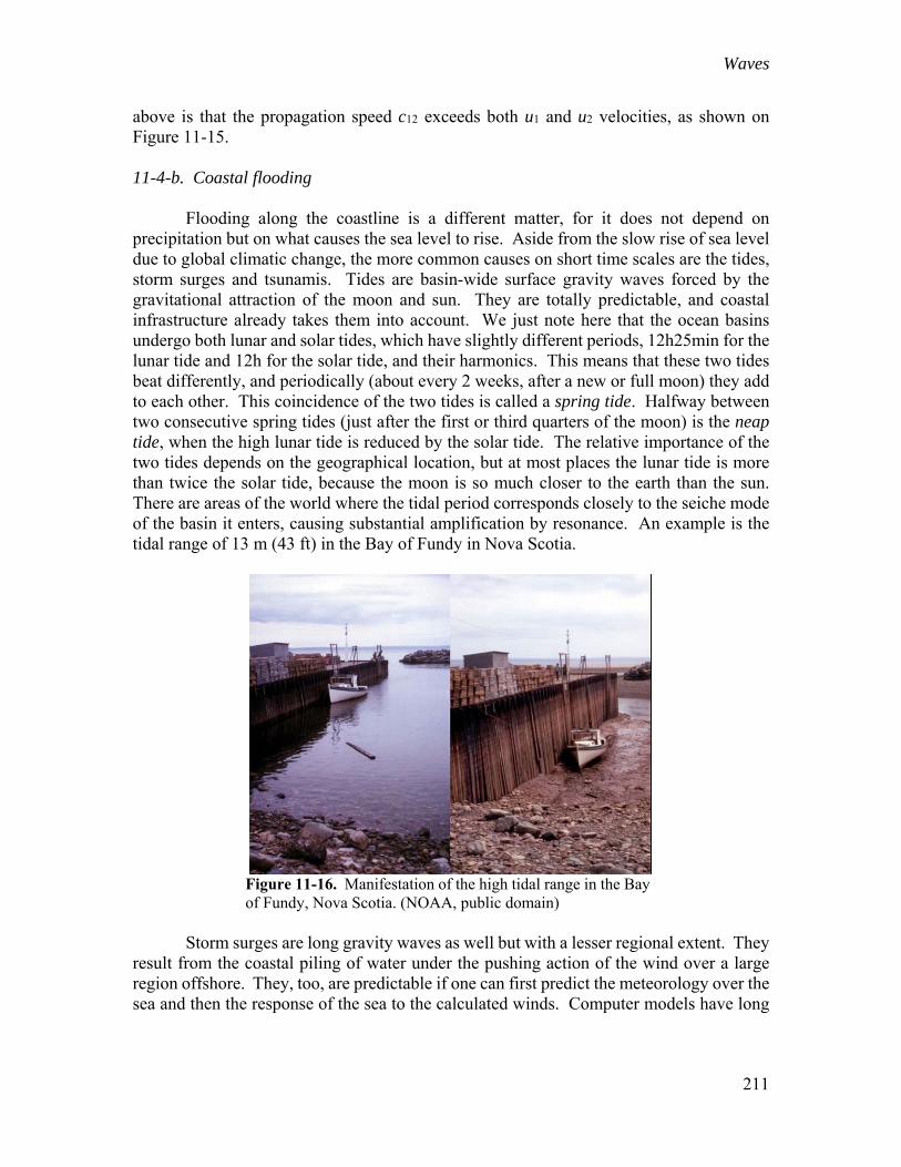
above is that the propagation speed c12 exceeds both u1 and u2 velocities, as shown on Figure 11-15. 11-4-b. Coastal flooding Flooding along the coastline is a different matter, for it does not depend on precipitation but on what causes the sea level to rise. Aside from the slow rise of sea level due to global climatic change, the more common causes on short time scales are the tides, storm surges and tsunamis. Tides are basin-wide surface gravity waves forced by the gravitational attraction of the moon and sun. They are totally predictable, and coastal infrastructure already takes them into account. We just note here that the ocean basins undergo both lunar and solar tides, which have slightly different periods, 12h25min for the lunar tide and 12h for the solar tide, and their harmonics. This means that these two tides beat differently, and periodically (about every 2 weeks, after a new or full moon) they add to each other. This coincidence of the two tides is called a spring tide. Halfway between two consecutive spring tides (just after the first or third quarters of the moon) is the neap tide, when the high lunar tide is reduced by the solar tide. The relative importance of the two tides depends on the geographical location, but at most places the lunar tide is more than twice the solar tide, because the moon is so much closer to the earth than the sun. There are areas of the world where the tidal period corresponds closely to the seiche mode of the basin it enters, causing substantial amplification by resonance. An example is the tidal range of 13 m (43 ft) in the Bay of Fundy in Nova Scotia.

Figure 11-16. Manifestation of the high tidal range in the Bay of Fundy, Nova Scotia. (NOAA, public domain)

Storm surges are long gravity waves as well but with a lesser regional extent. They result from the coastal piling of water under the pushing action of the wind over a large region offshore. They, too, are predictable if one can first predict the meteorology over the sea and then the response of the sea to the calculated winds. Computer models have long

Waves

212

existed8 to perform this twin set of tasks (ref here). A crucial element of these models is the value of the drag coefficient used in determining the wind stress on the water surface form the wind speed. The calculation then adds the tidal elevation. Such forecasting is essential in areas such as The Netherlands where lives are at risk and Venice where a UNESCO-designated architectural heritage is at stake. There is always the risk that a storm surge will coincide with a spring tide. The Dutch experienced such a coincidence and a disastrous flood in early 1953, which they have since called de Watersnoodramp (literally the nasty water disaster). It was in a sense a perfect storm: A sustained northerly wind over the North Sea in the last few days of January generated an unusually large storm surge, the arrival of which on the Dutch coastline coincided with the spring tide. Furthermore, the height of the storm surge occurred on the night of Saturday to Sunday when people were asleep. The Meteorology Institute saw the storm coming, but radios did not broadcast during the night, and government offices were empty for the weekend. So, the populace was not notified. The storm surge caused the water level to rise more than 5.6 m (18.4 ft) above mean sea level in some locations. Dikes were unable to resist the onslaught of the massive wave and were breached at dozens of locations. Casualties were numerous: 1,835 people and 30,000 animals lost their lives. The large areas of farmland inundated by seawater took years to be productive again. The Dutch swore that this would not be allowed to occur once again, and they built a large and comprehensive infrastructure, called Deltawerken (Delta Works, declared to be one of the Seven Wonders of the Modern World), some with opening and closing gates, to protect the land, much of which lies below mean sea level. In this context, predictive computer models play an essential role to instruct operators when to close the gates. The rule in practice is that the gates are closed whenever the sea level rises 3 m or more above mean sea level. The system has been activated a total of 27 times between completion in 1986 and January 2018. Venice is an interesting case as it sits at the northern end of the Adriatic Sea, which is an elongated basin with mountain chains on both flanks. It is also the site of some of the highest tides in the entire Mediterranean Sea and, having been built on mud, it slowly sinks under its own weight. The sirocco is a prevailing seasonal wind that is funneled between the coastal mountains and blows toward Venice generally between autumn and spring. When the sirocco persists for a few days, the storm surge it generates can raise the water level in Venice by more than 80 cm, occasionally more than 1 m. The spring tide in Venice is 93 cm. Acqua alta (high water) happens when both coincide, and major sections of Venice are under water. Moreover, the fundamental seiche mode of the Adriatic basin has a period of 21.5h, close to twice the periods of the lunar and solar tides. When the initial storm surge retreats, it is only to bounce back 21.5h later, as the water in the basin sloshes back and forth multiple times. So, if the initial surge did not coincide with the high tide, there is a chance that it will when it recurs. A single storm has multiple shots at hitting Venice!

8 Oceanographic models of storm surges were already developed in the 1970s, in the early days of research

computing.

Waves

213

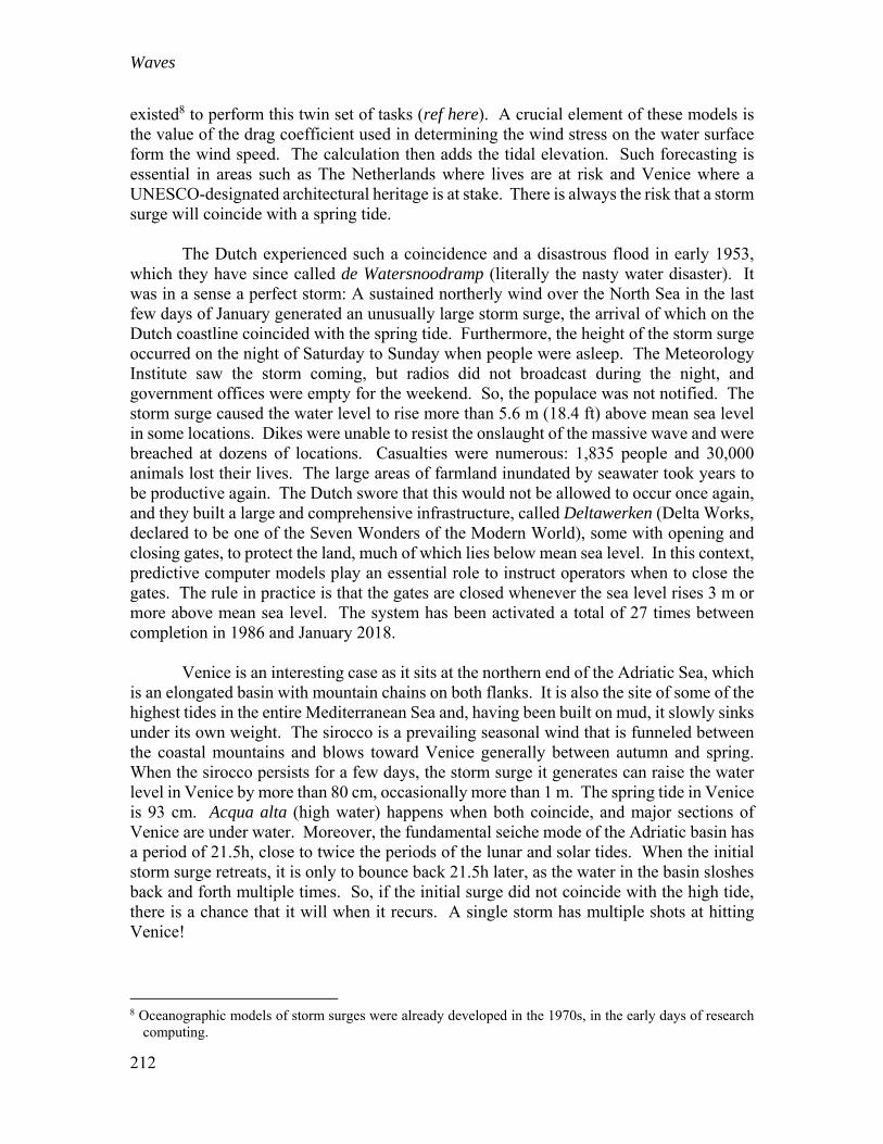
Figure 11-17. People walking in waist-high water in Venice’s main square on 29 October 2018. (Photo: Manuel Silvestri/Reuters)

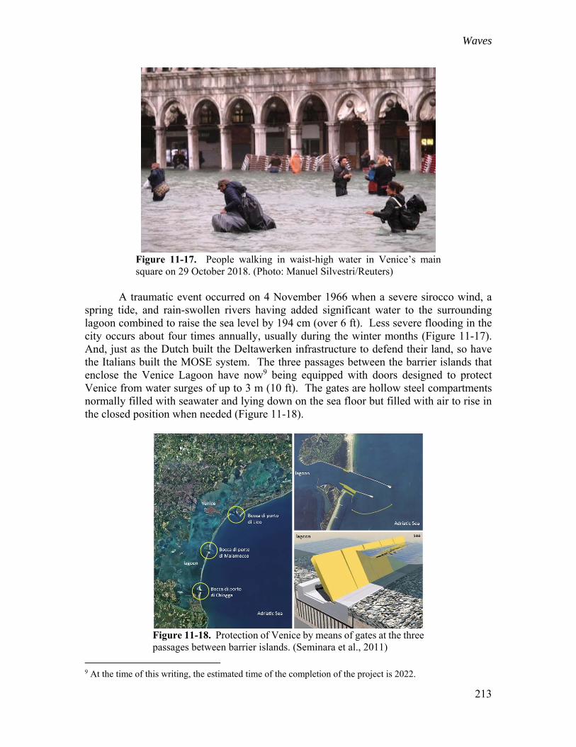
A traumatic event occurred on 4 November 1966 when a severe sirocco wind, a spring tide, and rain-swollen rivers having added significant water to the surrounding lagoon combined to raise the sea level by 194 cm (over 6 ft). Less severe flooding in the city occurs about four times annually, usually during the winter months (Figure 11-17). And, just as the Dutch built the Deltawerken infrastructure to defend their land, so have the Italians built the MOSE system. The three passages between the barrier islands that enclose the Venice Lagoon have now9 being equipped with doors designed to protect Venice from water surges of up to 3 m (10 ft). The gates are hollow steel compartments normally filled with seawater and lying down on the sea floor but filled with air to rise in the closed position when needed (Figure 11-18).

Figure 11-18. Protection of Venice by means of gates at the three passages between barrier islands. (Seminara et al., 2011)

9 At the time of this writing, the estimated time of the completion of the project is 2022.

Waves

214

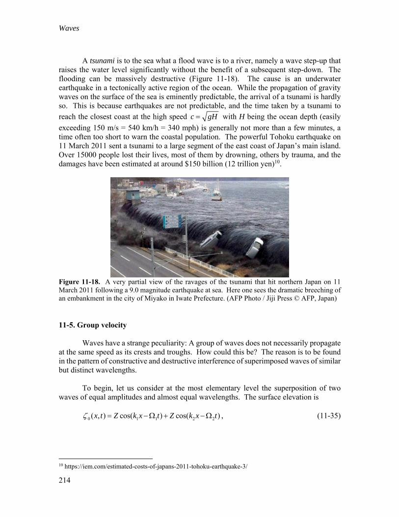
A tsunami is to the sea what a flood wave is to a river, namely a wave step-up that raises the water level significantly without the benefit of a subsequent step-down. The flooding can be massively destructive (Figure 11-18). The cause is an underwater earthquake in a tectonically active region of the ocean. While the propagation of gravity waves on the surface of the sea is eminently predictable, the arrival of a tsunami is hardly so. This is because earthquakes are not predictable, and the time taken by a tsunami to

reach the closest coast at the high speed c gH with H being the ocean depth (easily

exceeding 150 m/s = 540 km/h = 340 mph) is generally not more than a few minutes, a time often too short to warn the coastal population. The powerful Tohoku earthquake on 11 March 2011 sent a tsunami to a large segment of the east coast of Japan’s main island. Over 15000 people lost their lives, most of them by drowning, others by trauma, and the damages have been estimated at around $150 billion (12 trillion yen)10.

Figure 11-18. A very partial view of the ravages of the tsunami that hit northern Japan on 11 March 2011 following a 9.0 magnitude earthquake at sea. Here one sees the dramatic breeching of an embankment in the city of Miyako in Iwate Prefecture. (AFP Photo / Jiji Press © AFP, Japan) 11-5. Group velocity Waves have a strange peculiarity: A group of waves does not necessarily propagate at the same speed as its crests and troughs. How could this be? The reason is to be found in the pattern of constructive and destructive interference of superimposed waves of similar but distinct wavelengths. To begin, let us consider at the most elementary level the superposition of two waves of equal amplitudes and almost equal wavelengths. The surface elevation is 0 1 1 2 2( , ) cos( ) cos( )x t Z k x t Z k x t , (11-35)

10 https://iem.com/estimated-costs-of-japans-2011-tohoku-earthquake-3/

Waves

215

in which the two wavenumbers k1 and k2 are close to each other but not equal, and the two frequencies 1 and 2 are given in terms of the dispersion relation for the respective wavenumbers: ( ), 1, 2i i ik c k i . (11-36)

They, too, are close to each other but not equal. Using trigonometric relations, the sum of cosines in (11-35) can be recast as a product of cosines:

2 1 2 1 2 1 2 10 ( , ) 2 cos cos

2 2 2 2

k k k kx t Z x t x t

. (11-37)

Although this seems to complicate matters, it reveals something interesting: The wave amplitude 0 may now be viewed as a single wave with the average wavenumber and average frequency, as seen in the last cosine factor, with an amplitude made of the combination of the front factors,

2 1 2 12 cos2 2

k kZ x t

, (11-38)

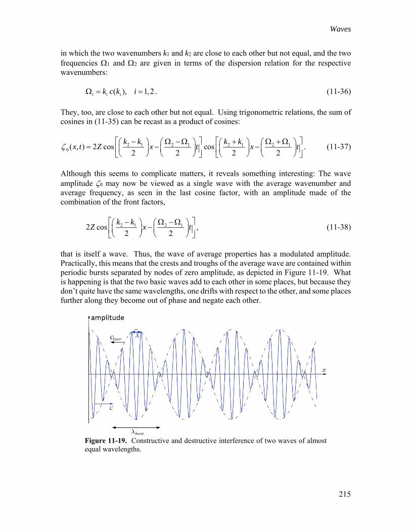
that is itself a wave. Thus, the wave of average properties has a modulated amplitude. Practically, this means that the crests and troughs of the average wave are contained within periodic bursts separated by nodes of zero amplitude, as depicted in Figure 11-19. What is happening is that the two basic waves add to each other in some places, but because they don’t quite have the same wavelengths, one drifts with respect to the other, and some places further along they become out of phase and negate each other.

Figure 11-19. Constructive and destructive interference of two waves of almost equal wavelengths.

Waves

216

If you were now asked: Where is the energy? You would most likely answer that it is confined within each burst because that is where the waves are at their greatest, and you would be right. Now these bursts travel with the speed of propagation of the amplitude (11-38), which is

2 1

2 1

2 1 2 1

2

2

burstck k k k k

. (11-39)

The wavelength of the bursts may be taken as the width of one:

2 1

1 2 2

2burstburstk k k

. (11-40)

Since the two wavenumbers are close to each other, their difference is small, and the burst is fairly wide, containing a significant number of elementary waves. In reality, waves don’t come in neat pairs as in the previous example but in collections of many wavelengths. The sum of two terms in (11-35) should really have been an infinite summation, that is, an integral covering a continuous spectrum of waves:

max

min0 ( , ) ( ) cos( )

k

kx t Z k kx t dk , (11-41)

in which the product Z(k)dk is the wave amplitude in the range from k to k+dk. Of this broad spectrum, let us isolate a narrow group of waves with wavenumbers ranging from k0–k to k0+k, centered on k0 with k small. Within that narrow interval, the variation of the frequency (k) (from the dispersion relation) is minor, and a Taylor expansion is permissible: 0 0( ) ( )k k k (11-42)

with 0 = (k0), and /d dk . The narrow group of waves can be approximated as:

0 0

0 00 0 0( ) cos( ) ( )cos ( ) ( )( )

k k k k

k k k kZ k kx t dk Z k k x t k k x t dk

0

00 0 0( ) cos ( )( ) cos( )

k k

k kZ k k k x t dk k x t

. (11-43)

(In the last manipulation, the sine term was dropped because its argument is small.) We note that this narrow group of waves can be described as a single wave of middle wavenumber k0 and frequency 0 with an amplitude (term inside braces) that travels at speed /d dk . If we now add all such groups together to reconstruct the full wave

Waves

217

field, we can describe what is happening as the summation of wave groups, each traveling with speed

g

dc

dk

(11-44)

corresponding to its middle wavenumber. The quantity cg is called the group velocity. Let us now apply this to deep-water gravity waves with frequency obtained from the dispersion relation (11-23),

( ) ( )k c k k gk , (11-45)

which yields:

1

2 2g

d g cc

dk k

. (11-46)

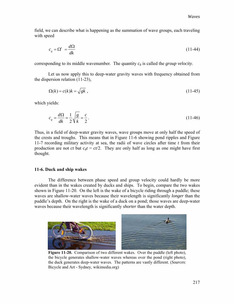
Thus, in a field of deep-water gravity waves, wave groups move at only half the speed of the crests and troughs. This means that in Figure 11-6 showing pond ripples and Figure 11-7 recording military activity at sea, the radii of wave circles after time t from their production are not ct but cgt = ct/2. They are only half as long as one might have first thought. 11-6. Duck and ship wakes The difference between phase speed and group velocity could hardly be more evident than in the wakes created by ducks and ships. To begin, compare the two wakes shown in Figure 11-20. On the left is the wake of a bicycle riding through a puddle; these waves are shallow-water waves because their wavelength is significantly longer than the puddle’s depth. On the right is the wake of a duck on a pond; those waves are deep-water waves because their wavelength is significantly shorter than the water depth.

Figure 11-20. Comparison of two different wakes. Over the puddle (left photo), the bicycle generates shallow-water waves whereas over the pond (right photo), the duck generates deep-water waves. The patterns are vastly different. (Sources: Bicycle and Art - Sydney, wikimedia.org)

Waves

218

We note that the shallow-water waves on the puddle form two well defined triangular wedges, one originating from each wheel. The waves all travel at speed

c gH and radiate away from each contact point between wheel and water. Over time

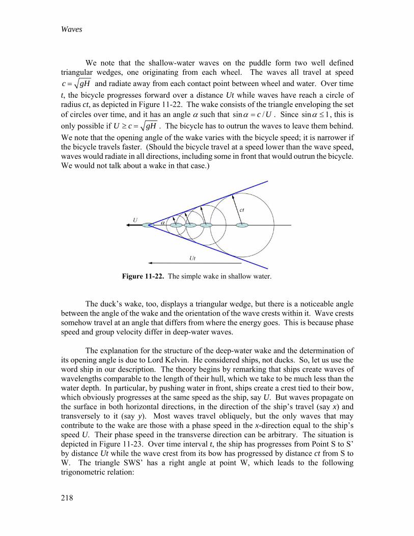
t, the bicycle progresses forward over a distance Ut while waves have reach a circle of radius ct, as depicted in Figure 11-22. The wake consists of the triangle enveloping the set of circles over time, and it has an angle such that sin /c U . Since sin 1 , this is

only possible if U c gH . The bicycle has to outrun the waves to leave them behind.

We note that the opening angle of the wake varies with the bicycle speed; it is narrower if the bicycle travels faster. (Should the bicycle travel at a speed lower than the wave speed, waves would radiate in all directions, including some in front that would outrun the bicycle. We would not talk about a wake in that case.)

Figure 11-22. The simple wake in shallow water.

The duck’s wake, too, displays a triangular wedge, but there is a noticeable angle between the angle of the wake and the orientation of the wave crests within it. Wave crests somehow travel at an angle that differs from where the energy goes. This is because phase speed and group velocity differ in deep-water waves. The explanation for the structure of the deep-water wake and the determination of its opening angle is due to Lord Kelvin. He considered ships, not ducks. So, let us use the word ship in our description. The theory begins by remarking that ships create waves of wavelengths comparable to the length of their hull, which we take to be much less than the water depth. In particular, by pushing water in front, ships create a crest tied to their bow, which obviously progresses at the same speed as the ship, say U. But waves propagate on the surface in both horizontal directions, in the direction of the ship’s travel (say x) and transversely to it (say y). Most waves travel obliquely, but the only waves that may contribute to the wake are those with a phase speed in the x-direction equal to the ship’s speed U. Their phase speed in the transverse direction can be arbitrary. The situation is depicted in Figure 11-23. Over time interval t, the ship has progresses from Point S to S’ by distance Ut while the wave crest from its bow has progressed by distance ct from S to W. The triangle SWS’ has a right angle at point W, which leads to the following trigonometric relation:

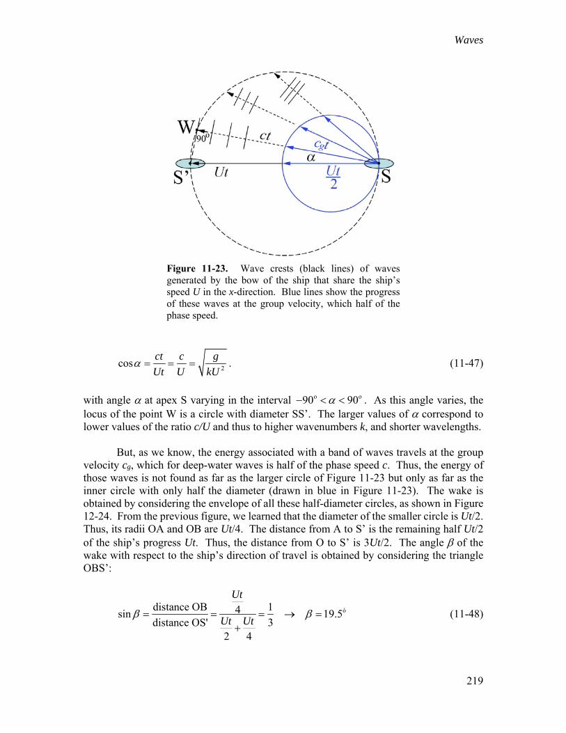
Waves

219

Figure 11-23. Wave crests (black lines) of waves generated by the bow of the ship that share the ship’s speed U in the x-direction. Blue lines show the progress of these waves at the group velocity, which half of the phase speed.

2

cosct c g

Ut U kU . (11-47)

with angle at apex S varying in the interval o o90 90 . As this angle varies, the locus of the point W is a circle with diameter SS’. The larger values of correspond to lower values of the ratio c/U and thus to higher wavenumbers k, and shorter wavelengths. But, as we know, the energy associated with a band of waves travels at the group velocity cg, which for deep-water waves is half of the phase speed c. Thus, the energy of those waves is not found as far as the larger circle of Figure 11-23 but only as far as the inner circle with only half the diameter (drawn in blue in Figure 11-23). The wake is obtained by considering the envelope of all these half-diameter circles, as shown in Figure 12-24. From the previous figure, we learned that the diameter of the smaller circle is Ut/2. Thus, its radii OA and OB are Ut/4. The distance from A to S’ is the remaining half Ut/2 of the ship’s progress Ut. Thus, the distance from O to S’ is 3Ut/2. The angle of the wake with respect to the ship’s direction of travel is obtained by considering the triangle OBS’:

ódistance OB 14sin 19.5distance OS' 3

2 4

Ut

Ut Ut

(11-48)

Waves

220

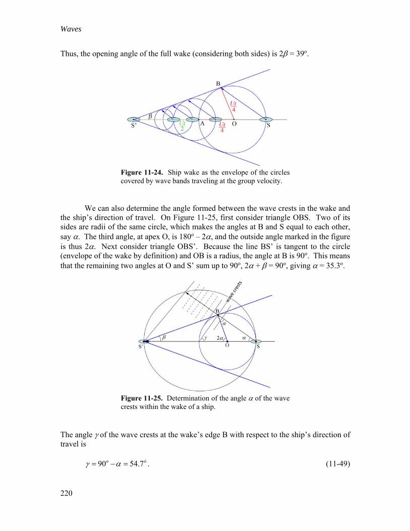
Thus, the opening angle of the full wake (considering both sides) is 2 = 39o.

Figure 11-24. Ship wake as the envelope of the circles covered by wave bands traveling at the group velocity.

We can also determine the angle formed between the wave crests in the wake and the ship’s direction of travel. On Figure 11-25, first consider triangle OBS. Two of its sides are radii of the same circle, which makes the angles at B and S equal to each other, say . The third angle, at apex O, is 180o – 2, and the outside angle marked in the figure is thus 2. Next consider triangle OBS’. Because the line BS’ is tangent to the circle (envelope of the wake by definition) and OB is a radius, the angle at B is 90o. This means that the remaining two angles at O and S’ sum up to 90o, 2 + = 90o, giving = 35.3o.

Figure 11-25. Determination of the angle of the wave crests within the wake of a ship.

The angle of the wave crests at the wake’s edge B with respect to the ship’s direction of travel is ó90 54.7o . (11-49)

Waves

221

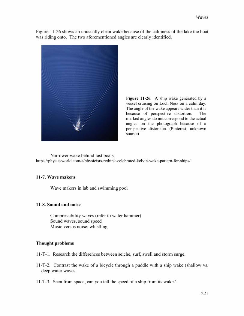
Figure 11-26 shows an unusually clean wake because of the calmness of the lake the boat was riding onto. The two aforementioned angles are clearly identified.

Figure 11-26. A ship wake generated by a vessel cruising on Loch Ness on a calm day. The angle of the wake appears wider than it is because of perspective distortion. The marked angles do not correspond to the actual angles on the photograph because of a perspective distorsion. (Pinterest, unknown source)

Narrower wake behind fast boats. https://physicsworld.com/a/physicists-rethink-celebrated-kelvin-wake-pattern-for-ships/ 11-7. Wave makers Wave makers in lab and swimming pool 11-8. Sound and noise Compressibility waves (refer to water hammer) Sound waves, sound speed Music versus noise; whistling Thought problems 11-T-1. Research the differences between seiche, surf, swell and storm surge. 11-T-2. Contrast the wake of a bicycle through a puddle with a ship wake (shallow vs.

deep water waves. 11-T-3. Seen from space, can you tell the speed of a ship from its wake?

Waves

222

Quantitative Exercises 11-Q-1. Question

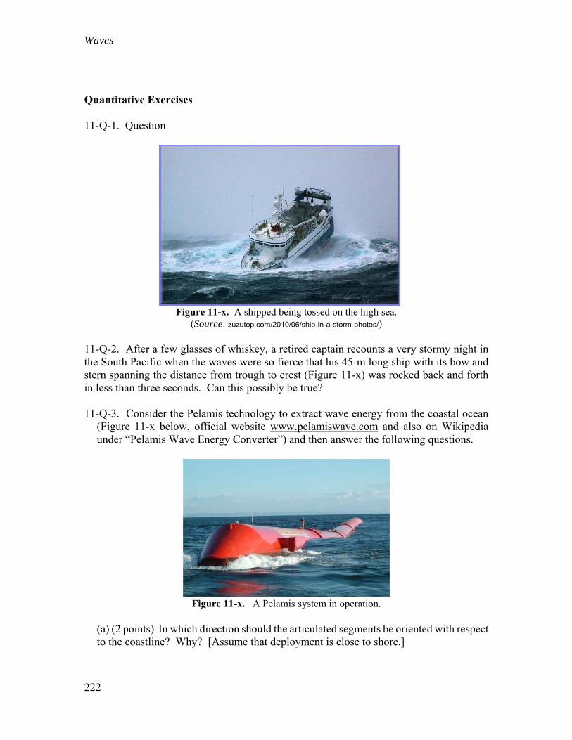
Figure 11-x. A shipped being tossed on the high sea.

(Source: zuzutop.com/2010/06/ship-in-a-storm-photos/)

11-Q-2. After a few glasses of whiskey, a retired captain recounts a very stormy night in the South Pacific when the waves were so fierce that his 45-m long ship with its bow and stern spanning the distance from trough to crest (Figure 11-x) was rocked back and forth in less than three seconds. Can this possibly be true? 11-Q-3. Consider the Pelamis technology to extract wave energy from the coastal ocean

(Figure 11-x below, official website www.pelamiswave.com and also on Wikipedia under “Pelamis Wave Energy Converter”) and then answer the following questions.

Figure 11-x. A Pelamis system in operation.

(a) (2 points) In which direction should the articulated segments be oriented with respect

to the coastline? Why? [Assume that deployment is close to shore.]

Waves

223

(b) (2 points) A typical deployment consists of an assembly of 4 segments for a total length of 150 meters. At what surface-wave wavelength is the device most efficient at extracting energy?

(c) (2 points) What happens if the wavelength is twice as long and half as long as the value obtained above? Assume a sinusoidal wave shape.

(d) (4 points) Forecast for Hawai’i (www.stormsurfing.com/cgi/display.cgi?a=hi_per) indicates that the wave period on the south side of the Island of Oahu (where Honolulu and Waikiki are situated) ranges between 10 and 15 seconds. In what range of water depth should a Pelamis system be deployed south of Oahu?