Embed Size (px)
Citation preview
Chapter 11: N2O Emissions from Managed Soils, and CO2 Emissions from Lime and Urea Application
2006 IPCC Guidelines for National Greenhouse Gas Inventories 11.1
C H A P T E R 1 1
N2O EMISSIONS FROM MANAGED SOILS, AND CO2 EMISSIONS FROM LIME AND UREA APPLICATION
Volume 4: Agriculture, Forestry and Other Land Use
11.2 2006 IPCC Guidelines for National Greenhouse Gas Inventories
Authors Cecile De Klein (New Zealand), Rafael S.A. Novoa (Chile), Stephen Ogle (USA), Keith A. Smith (UK), Philippe Rochette (Canada), and Thomas C. Wirth (USA)
Brian G. McConkey (Canada), Arvin Mosier (USA), and Kristin Rypdal (Norway)
Contributing Authors Margaret Walsh (USA) and Stephen A. Williams (USA)
Chapter 11: N2O Emissions from Managed Soils, and CO2 Emissions from Lime and Urea Application
2006 IPCC Guidelines for National Greenhouse Gas Inventories 11.3
Contents
11 N2O Emissions from Managed Soils, and CO2 Emissions from Lime and Urea Application
11.1 Introduction .........................................................................................................................................11.5 11.2 N2O Emissions from Managed Soils...................................................................................................11.5
11.2.1 Direct N2O emissions ..................................................................................................................11.6 11.2.1.1 Choice of method...................................................................................................................11.6 11.2.1.2 Choice of emission factors...................................................................................................11.10 11.2.1.3 Choice of activity data .........................................................................................................11.12 11.2.1.4 Uncertainty assessment........................................................................................................11.16
11.2.2 Indirect N2O emissions..............................................................................................................11.19 11.2.2.1 Choice of method.................................................................................................................11.19 11.2.2.2 Choice of emission, volatilisation and leaching factors.......................................................11.23 11.2.2.3 Choice of activity data .........................................................................................................11.23 11.2.2.4 Uncertainty assessment........................................................................................................11.24
11.2.3 Completeness, Time series, QA/QC..........................................................................................11.25 11.3 CO2 Emissions from Liming .............................................................................................................11.26
11.3.1 Choice of method ......................................................................................................................11.27 11.3.2 Choice of emission factors ........................................................................................................11.29 11.3.3 Choice of activity data...............................................................................................................11.29 11.3.4 Uncertainty assessment .............................................................................................................11.29 11.3.5 Completeness, Time series, QA/QC..........................................................................................11.30
11.4 CO2 Emissions from Urea Fertilization.............................................................................................11.32 11.4.1 Choice of method ......................................................................................................................11.32 11.4.2 Choice of emission factor..........................................................................................................11.34 11.4.3 Choice of activity data...............................................................................................................11.34 11.4.4 Uncertainty assessment .............................................................................................................11.34 11.4.5 Completeness, Time series consistency, QA/QC ......................................................................11.35
Annex 11A.1 References for crop residue data in Table 11.2 .........................................................................11.37 References ...................................................................................................................................................11.53
Volume 4: Agriculture, Forestry and Other Land Use
11.4 2006 IPCC Guidelines for National Greenhouse Gas Inventories
Equations
Equation 11.1 Direct N2O emissions from managed soils (Tier 1).............................................................11.7 Equation 11.2 Direct N2O emissions from managed soils (Tier 2)...........................................................11.10 Equation 11.3 N from organic N additions applied to soils (Tier 1).........................................................11.12 Equation 11.4 N from animal manure applied to soils (Tier 1) ................................................................11.13 Equation 11.5 N in urine and dung deposited by grazing animals on pasture,
range and paddock (Tier 1)................................................................................................11.13 Equation 11.6 N from crop residues and forage/pasture renewal (Tier 1) ................................................11.14 Equation 11.7 Dry-weight correction of reported crop yields ..................................................................11.15 Equation 11.7A Alternative approach to estimate FCR (using Table 11.2) ..................................................11.15 Equation 11.8 N mineralised in mineral soils as a result of loss of soil C through change
in land use or management (Tiers 1 and 2)........................................................................11.16 Equation 11.9 N2O from atmospheric deposition of N volatilised from managed soils (Tier 1) ..............11.21 Equation 11.10 N2O from N leaching/runoff from managed soils in regions where leaching/runoff
occurs (Tier 1) ...................................................................................................................11.21 Equation 11.11 N2O from atmospheric deposition of N volatilised from managed soils (Tier 2) ..............11.22 Equation 11.12 Annual CO2 emissions from lime application ...................................................................11.27 Equation 11.13 Annual CO2 emissions from urea application....................................................................11.32
Figures
Figure 11.1 Schematic diagram illustrating the sources and pathways of N that result in direct and indirect N2O emissions from soils and waters. ...............................................11.8
Figure 11.2 Decision tree for direct N2O emissions from managed soils ...............................................11.9 Figure 11.3 Decision tree for indirect N2O emissions from managed soils ..........................................11.20 Figure 11.4 Decision tree for identification of appropriate tier to estimate CO2 emissions
from liming........................................................................................................................11.28 Figure 11.5 Decision tree for identification of appropriate tier to estimate CO2 emissions
from urea fertilisation ........................................................................................................11.33
Tables
Table 11.1 Default emission factors to estimate direct N2O emissions from managed soils...............11.11 Table 11.2 Default factors for estimation of N added to soils from crop residues ..............................11.17 Table 11.3 Default emission, volatilisation and leaching factors for indirect soil N2O emissions ......11.24
Chapter 11: N2O Emissions from Managed Soils, and CO2 Emissions from Lime and Urea Application
2006 IPCC Guidelines for National Greenhouse Gas Inventories 11.5
11 N2O EMISSIONS FROM MANAGED SOILS, AND CO2 EMISSIONS FROM LIME AND UREA APPLICATION
11.1 INTRODUCTION Chapter 11 provides a description of the generic methodologies to be adopted for the inventory of nitrous oxide (N2O) emissions from managed soils, including indirect N2O emissions from additions of N to land due to deposition and leaching, and emissions of carbon dioxide (CO2) following additions of liming materials and urea-containing fertiliser.
Managed soils1 are all soils on land, including Forest Land, which is managed. For N2O, the basic three-tier approach is the same as used in the IPCC Good Practice Guidance for Land Use, Land-use Change and Forestry (GPG-LULUCF) for Grassland and Cropland, and in the IPCC Good Practice Guidance and Uncertainty Management in National Greenhouse Gas Inventories (GPG2000) for agricultural soils while relevant parts of the GPG-LULUCF methodology have been included for Forest Land. Because the methods are based on pools and fluxes that can occur in all the different land-use categories and because in most cases, only national aggregate (i.e., non-land use specific) data are available, generic information on the methodologies, as applied at the national level is given here, including:
• a general framework for applying the methods, and appropriate equations for the calculations;
• an explanation of the processes governing N2O emissions from managed soils (direct and indirect) and CO2 emissions from liming and urea fertilisation, and the associated uncertainties; and
• choice of methods, emission factors (including default values) and activity data, and volatilisation and leaching factors.
• If activity data are available for specific land-use categories, the equations provided can be implemented for specific land-use categories.
The changes in the 2006 IPCC Guidelines, relative to 1996 IPCC Guidelines, include the following:
• provision of advice on estimating CO2 emissions associated with the use of urea as a fertilizer;
• full sectoral coverage of indirect N2O emissions;
• extensive literature review leading to revised emission factors for nitrous oxide from agricultural soils; and
• removal of biological nitrogen fixation as a direct source of N2O because of the lack of evidence of significant emissions arising from the fixation process.
11.2 N2O EMISSIONS FROM MANAGED SOILS This section presents the methods and equations for estimating total national anthropogenic emissions of N2O (direct and indirect) from managed soils. The generic equations presented here can also be used for estimating N2O within specific land-use categories or by condition-specific variables (e.g., N additions to rice paddies) if the country can disaggregate the activity data to that level (i.e., N use activity within a specific land use).
Nitrous oxide is produced naturally in soils through the processes of nitrification and denitrification. Nitrification is the aerobic microbial oxidation of ammonium to nitrate, and denitrification is the anaerobic microbial reduction of nitrate to nitrogen gas (N2). Nitrous oxide is a gaseous intermediate in the reaction sequence of denitrification and a by-product of nitrification that leaks from microbial cells into the soil and ultimately into the atmosphere. One of the main controlling factors in this reaction is the availability of inorganic N in the soil. This methodology, therefore, estimates N2O emissions using human-induced net N additions to soils (e.g., synthetic or organic fertilisers, deposited manure, crop residues, sewage sludge), or of mineralisation of N in soil organic matter following drainage/management of organic soils, or cultivation/land-use change on mineral soils (e.g., Forest Land/Grassland/Settlements converted to Cropland).
1 Managed land is defined in Chapter 1, Section 1.1.
Volume 4: Agriculture, Forestry and Other Land Use
11.6 2006 IPCC Guidelines for National Greenhouse Gas Inventories
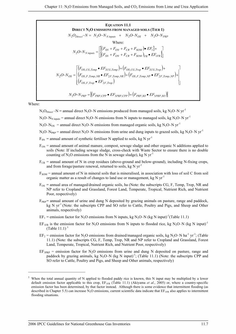
The emissions of N2O that result from anthropogenic N inputs or N mineralisation occur through both a direct pathway (i.e., directly from the soils to which the N is added/released), and through two indirect pathways: (i) following volatilisation of NH3 and NOx from managed soils and from fossil fuel combustion and biomass burning, and the subsequent redeposition of these gases and their products NH4
+ and NO3- to soils and waters;
and (ii) after leaching and runoff of N, mainly as NO3-, from managed soils. The principal pathways are
illustrated in Figure 11.1.
Direct emissions of N2O from managed soils are estimated separately from indirect emissions, though using a common set of activity data. The Tier 1 methodologies do not take into account different land cover, soil type, climatic conditions or management practices (other than specified above). Neither do they take account of any lag time for direct emissions from crop residues N, and allocate these emissions to the year in which the residues are returned to the soil. These factors are not considered for direct or (where appropriate, indirect) emissions because limited data are available to provide appropriate emission factors. Countries that have data to show that default factors are inappropriate for their country should utilise Tier 2 equations or Tier 3 approaches and include a full explanation for the values used.
11.2.1 Direct N2O emissions In most soils, an increase in available N enhances nitrification and denitrification rates which then increase the production of N2O. Increases in available N can occur through human-induced N additions or change of land-use and/or management practices that mineralise soil organic N.
The following N sources are included in the methodology for estimating direct N2O emissions from managed soils:
• synthetic N fertilisers (FSN);
• organic N applied as fertiliser (e.g., animal manure, compost, sewage sludge, rendering waste) (FON);
• urine and dung N deposited on pasture, range and paddock by grazing animals (FPRP);
• N in crop residues (above-ground and below-ground), including from N-fixing crops 2 and from forages during pasture renewal 3 (FCR);
• N mineralisation associated with loss of soil organic matter resulting from change of land use or management of mineral soils (FSOM); and
• drainage/management of organic soils (i.e., Histosols) 4 (FOS).
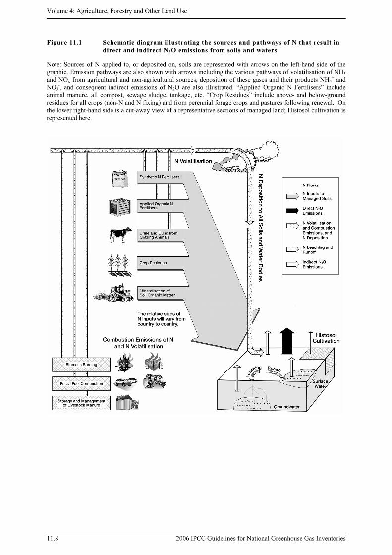
11.2.1.1 CHOICE OF METHOD The decision tree in Figure 11.2 provides guidance on which tier method to use.
Tier 1 In its most basic form, direct N2O emissions from managed soils are estimated using Equation 11.1 as follows:
2 Biological nitrogen fixation has been removed as a direct source of N2O because of the lack of evidence of significant
emissions arising from the fixation process itself (Rochette and Janzen, 2005). These authors concluded that the N2O emissions induced by the growth of legume crops/forages may be estimated solely as a function of the above-ground and below-ground nitrogen inputs from crop/forage residue (the nitrogen residue from forages is only accounted for during pasture renewal). Conversely, the release of N by mineralisation of soil organic matter as a result of change of land use or management is now included as an additional source. These are significant adjustments to the methodology previously described in the 1996 IPCC Guidelines.
3 The nitrogen residue from perennial forage crops is only accounted for during periodic pasture renewal, i.e. not necessarily on an annual basis as is the case with annual crops.
4 Soils are organic if they satisfy the requirements 1 and 2, or 1 and 3 below (FAO, 1998): 1. Thickness of 10 cm or more. A horizon less than 20 cm thick must have 12 percent or more organic carbon when mixed to a depth of 20 cm; 2. If the soil is never saturated with water for more than a few days, and contains more than 20 percent (by weight) organic carbon (about 35 percent organic matter); 3. If the soil is subject to water saturation episodes and has either: (i) at least 12 percent (by weight) organic carbon (about 20 percent organic matter) if it has no clay; or (ii) at least 18 percent (by weight) organic carbon (about 30 percent organic matter) if it has 60 percent or more clay; or (iii) an intermediate, proportional amount of organic carbon for intermediate amounts of clay (FAO, 1998).
Chapter 11: N2O Emissions from Managed Soils, and CO2 Emissions from Lime and Urea Application
2006 IPCC Guidelines for National Greenhouse Gas Inventories 11.7
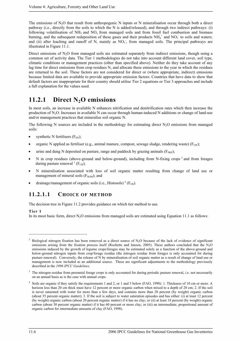
EQUATION 11.1 DIRECT N2O EMISSIONS FROM MANAGED SOILS (TIER 1)
PRPOSinputsNDirect NONNONNONNON −+−+−=− 2222
Where: ( )[ ]( )[ ]⎥⎦
⎤⎢⎣
⎡•+++
+•+++=−
FRFRSOMCRONSN
SOMCRONSNinputsN EFFFFF
EFFFFFNON
1
12
( ) ( )( ) ( )( ) ⎥
⎥⎥⎥
⎦
⎤
⎢⎢⎢⎢
⎣
⎡
•
+•+•
+•+•
=−
TropFTropFOS
NPTempFNPTempFOSNRTempFNRTempFOS
TropCGTropCGOSTempCGTempCGOS
OS
EFF
EFFEFF
EFFEFF
NON
,2,,
,,2,,,,,2,,,
,2,,,2,,
2
( ) ( )[ ]SOPRPSOPRPCPPPRPCPPPRPPRP EFFEFFNON ,3,,3,2 •+•=−
Where:
N2ODirect –N = annual direct N2O–N emissions produced from managed soils, kg N2O–N yr-1
N2O–NN inputs = annual direct N2O–N emissions from N inputs to managed soils, kg N2O–N yr-1
N2O–NOS = annual direct N2O–N emissions from managed organic soils, kg N2O–N yr-1
N2O–NPRP = annual direct N2O–N emissions from urine and dung inputs to grazed soils, kg N2O–N yr-1
FSN = annual amount of synthetic fertiliser N applied to soils, kg N yr-1
FON = annual amount of animal manure, compost, sewage sludge and other organic N additions applied to soils (Note: If including sewage sludge, cross-check with Waste Sector to ensure there is no double counting of N2O emissions from the N in sewage sludge), kg N yr-1
FCR = annual amount of N in crop residues (above-ground and below-ground), including N-fixing crops, and from forage/pasture renewal, returned to soils, kg N yr-1
FSOM = annual amount of N in mineral soils that is mineralised, in association with loss of soil C from soil organic matter as a result of changes to land use or management, kg N yr-1
FOS = annual area of managed/drained organic soils, ha (Note: the subscripts CG, F, Temp, Trop, NR and NP refer to Cropland and Grassland, Forest Land, Temperate, Tropical, Nutrient Rich, and Nutrient Poor, respectively)
FPRP = annual amount of urine and dung N deposited by grazing animals on pasture, range and paddock, kg N yr-1 (Note: the subscripts CPP and SO refer to Cattle, Poultry and Pigs, and Sheep and Other animals, respectively)
EF1 = emission factor for N2O emissions from N inputs, kg N2O–N (kg N input)-1(Table 11.1)
EF1FR is the emission factor for N2O emissions from N inputs to flooded rice, kg N2O–N (kg N input)-1
(Table 11.1) 5
EF2 = emission factor for N2O emissions from drained/managed organic soils, kg N2O–N ha-1 yr-1; (Table 11.1) (Note: the subscripts CG, F, Temp, Trop, NR and NP refer to Cropland and Grassland, Forest Land, Temperate, Tropical, Nutrient Rich, and Nutrient Poor, respectively)
EF3PRP = emission factor for N2O emissions from urine and dung N deposited on pasture, range and paddock by grazing animals, kg N2O–N (kg N input)-1; (Table 11.1) (Note: the subscripts CPP and SO refer to Cattle, Poultry and Pigs, and Sheep and Other animals, respectively)
5 When the total annual quantity of N applied to flooded paddy rice is known, this N input may be multiplied by a lower
default emission factor applicable to this crop, EF1FR (Table 11.1) (Akiyama et al., 2005) or, where a country-specific emission factor has been determined, by that factor instead. Although there is some evidence that intermittent flooding (as described in Chapter 5.5) can increase N2O emissions, current scientific data indicate that EF1FR also applies to intermittent flooding situations.
Volume 4: Agriculture, Forestry and Other Land Use
11.8 2006 IPCC Guidelines for National Greenhouse Gas Inventories
Figure 11.1 Schematic diagram illustrating the sources and pathways of N that result in direct and indirect N2O emissions from soils and waters
Note: Sources of N applied to, or deposited on, soils are represented with arrows on the left-hand side of the graphic. Emission pathways are also shown with arrows including the various pathways of volatilisation of NH3 and NOx from agricultural and non-agricultural sources, deposition of these gases and their products NH4
+ and NO3
-, and consequent indirect emissions of N2O are also illustrated. “Applied Organic N Fertilisers” include animal manure, all compost, sewage sludge, tankage, etc. “Crop Residues” include above- and below-ground residues for all crops (non-N and N fixing) and from perennial forage crops and pastures following renewal. On the lower right-hand side is a cut-away view of a representative sections of managed land; Histosol cultivation is represented here.
Chapter 11: N2O Emissions from Managed Soils, and CO2 Emissions from Lime and Urea Application
2006 IPCC Guidelines for National Greenhouse Gas Inventories 11.9
Figure 11.2 Decision tree for direct N2O emissions from managed soils
Start
Do youhave rigorously
documented country-specificemission factors
for EF1, EF2, and/orEF3PRP?
Obtain country-specific
data.
Estimate emissions using the Tier 1default emission factor value and
country-specific activity data.
No
Note:1: N sources include: synthetic N fertiliser, organic N additions, urine and dung deposited during grazing, crop/forage residue, mineralisation of N contained in soil organic matter that accompanies C loss from soils following a change in land use or management and drainage/management of organic soils. Other organic N additions (e.g., compost, sewage sludge, rendering waste) can be included in this calculation if sufficient information is available. The waste input is measured in units of N and added as an additional source sub-term under FON in Equation 11.1 to be multiplied by EF1.2: See Volume 1 Chapter 4, "Methodological Choice and Identification of Key Categories" (noting Section 4.1.2 on limited resources), for discussion of key categories and use of decision trees.3: As a rule of thumb, a sub-category would be significant if it accounts for 25-30% of emissions from the source category.
Is thisa key category2 and
is this N sourcesignificant3?
No
Yes
Estimate emissions using Tier 2equation and available country-
specific emission factors, or Tier 3 methods.
YesYes
Box 2: Tier 1
Box 1: Tier 1
No
Estimate emissions using Tier 1equations, default emission factors,
FAO activity data for mineral Nfertiliser use and livestock
populations, and expert opinion on other activity data.
Foreach N source ask:
Do you have country-specificactivity data1?
Box 3: Tier 2 or 3
Volume 4: Agriculture, Forestry and Other Land Use
11.10 2006 IPCC Guidelines for National Greenhouse Gas Inventories
Conversion of N2O–N emissions to N2O emissions for reporting purposes is performed by using the following equation:
N2O = N2O–N ● 44/28
Tier 2 If more detailed emission factors and corresponding activity data are available to a country than are presented in Equation 11.1, further disaggregation of the terms in the equation can be undertaken. For example, if emission factors and activity data are available for the application of synthetic fertilisers and organic N (FSN and FON) under different conditions i, Equation 11.1 would be expanded to become 6:
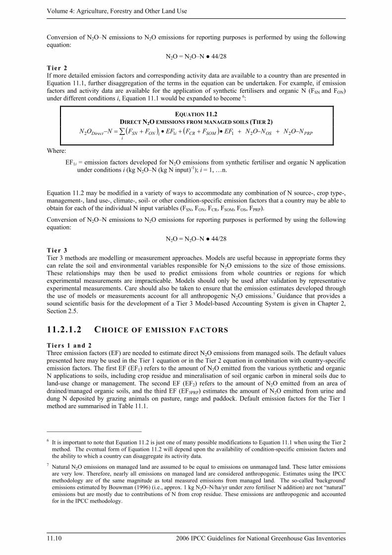
EQUATION 11.2 DIRECT N2O EMISSIONS FROM MANAGED SOILS (TIER 2)
( ) ( )∑ −+−+•++•+=−i
PRPOSSOMCRiiONSNDirect NONNONEFFFEFFFNON 22112
Where:
EF1i = emission factors developed for N2O emissions from synthetic fertiliser and organic N application under conditions i (kg N2O–N (kg N input)-1); i = 1, …n.
Equation 11.2 may be modified in a variety of ways to accommodate any combination of N source-, crop type-, management-, land use-, climate-, soil- or other condition-specific emission factors that a country may be able to obtain for each of the individual N input variables (FSN, FON, FCR, FSOM, FOS, FPRP).
Conversion of N2O–N emissions to N2O emissions for reporting purposes is performed by using the following equation:
N2O = N2O–N ● 44/28
Tier 3 Tier 3 methods are modelling or measurement approaches. Models are useful because in appropriate forms they can relate the soil and environmental variables responsible for N2O emissions to the size of those emissions. These relationships may then be used to predict emissions from whole countries or regions for which experimental measurements are impracticable. Models should only be used after validation by representative experimental measurements. Care should also be taken to ensure that the emission estimates developed through the use of models or measurements account for all anthropogenic N2O emissions.7 Guidance that provides a sound scientific basis for the development of a Tier 3 Model-based Accounting System is given in Chapter 2, Section 2.5.
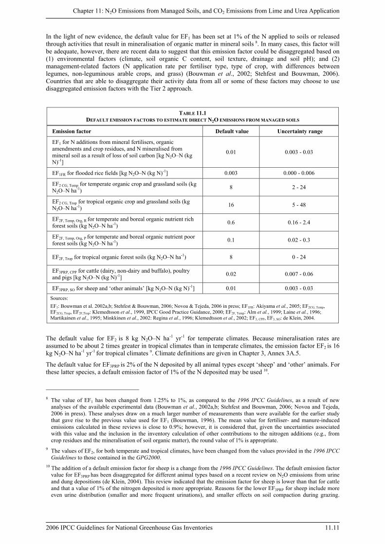
11.2.1.2 CHOICE OF EMISSION FACTORS
Tiers 1 and 2 Three emission factors (EF) are needed to estimate direct N2O emissions from managed soils. The default values presented here may be used in the Tier 1 equation or in the Tier 2 equation in combination with country-specific emission factors. The first EF (EF1) refers to the amount of N2O emitted from the various synthetic and organic N applications to soils, including crop residue and mineralisation of soil organic carbon in mineral soils due to land-use change or management. The second EF (EF2) refers to the amount of N2O emitted from an area of drained/managed organic soils, and the third EF (EF3PRP) estimates the amount of N2O emitted from urine and dung N deposited by grazing animals on pasture, range and paddock. Default emission factors for the Tier 1 method are summarised in Table 11.1.
6 It is important to note that Equation 11.2 is just one of many possible modifications to Equation 11.1 when using the Tier 2
method. The eventual form of Equation 11.2 will depend upon the availability of condition-specific emission factors and the ability to which a country can disaggregate its activity data.
7 Natural N2O emissions on managed land are assumed to be equal to emissions on unmanaged land. These latter emissions are very low. Therefore, nearly all emissions on managed land are considered anthropogenic. Estimates using the IPCC methodology are of the same magnitude as total measured emissions from managed land. The so-called 'background' emissions estimated by Bouwman (1996) (i.e., approx. 1 kg N2O–N/ha/yr under zero fertiliser N addition) are not “natural” emissions but are mostly due to contributions of N from crop residue. These emissions are anthropogenic and accounted for in the IPCC methodology.
Chapter 11: N2O Emissions from Managed Soils, and CO2 Emissions from Lime and Urea Application
2006 IPCC Guidelines for National Greenhouse Gas Inventories 11.11
In the light of new evidence, the default value for EF1 has been set at 1% of the N applied to soils or released through activities that result in mineralisation of organic matter in mineral soils 8. In many cases, this factor will be adequate, however, there are recent data to suggest that this emission factor could be disaggregated based on (1) environmental factors (climate, soil organic C content, soil texture, drainage and soil pH); and (2) management-related factors (N application rate per fertiliser type, type of crop, with differences between legumes, non-leguminous arable crops, and grass) (Bouwman et al., 2002; Stehfest and Bouwman, 2006). Countries that are able to disaggregate their activity data from all or some of these factors may choose to use disaggregated emission factors with the Tier 2 approach.
TABLE 11.1 DEFAULT EMISSION FACTORS TO ESTIMATE DIRECT N2O EMISSIONS FROM MANAGED SOILS
Emission factor Default value Uncertainty range
EF1 for N additions from mineral fertilisers, organic amendments and crop residues, and N mineralised from mineral soil as a result of loss of soil carbon [kg N2O–N (kg N)-1]
0.01 0.003 - 0.03
EF1FR for flooded rice fields [kg N2O–N (kg N)-1] 0.003 0.000 - 0.006
EF2 CG, Temp for temperate organic crop and grassland soils (kg N2O–N ha-1) 8 2 - 24
EF2 CG, Trop for tropical organic crop and grassland soils (kg N2O–N ha-1) 16 5 - 48
EF2F, Temp, Org, R for temperate and boreal organic nutrient rich forest soils (kg N2O–N ha-1) 0.6 0.16 - 2.4
EF2F, Temp, Org, P for temperate and boreal organic nutrient poor forest soils (kg N2O–N ha-1) 0.1 0.02 - 0.3
EF2F, Trop for tropical organic forest soils (kg N2O–N ha-1) 8 0 - 24
EF3PRP, CPP for cattle (dairy, non-dairy and buffalo), poultry and pigs [kg N2O–N (kg N)-1] 0.02 0.007 - 0.06
EF3PRP, SO for sheep and ‘other animals’ [kg N2O–N (kg N)-1] 0.01 0.003 - 0.03
Sources: EF1: Bouwman et al. 2002a,b; Stehfest & Bouwman, 2006; Novoa & Tejeda, 2006 in press; EF1FR: Akiyama et al., 2005; EF2CG, Temp, EF2CG, Trop, EF2F,Trop: Klemedtsson et al., 1999, IPCC Good Practice Guidance, 2000; EF2F, Temp: Alm et al., 1999; Laine et al., 1996; Martikainen et al., 1995; Minkkinen et al., 2002: Regina et al., 1996; Klemedtsson et al., 2002; EF3, CPP, EF3, SO: de Klein, 2004.
The default value for EF2 is 8 kg N2O–N ha-1 yr-1 for temperate climates. Because mineralisation rates are assumed to be about 2 times greater in tropical climates than in temperate climates, the emission factor EF2 is 16 kg N2O–N ha-1 yr-1 for tropical climates 9. Climate definitions are given in Chapter 3, Annex 3A.5.
The default value for EF3PRP is 2% of the N deposited by all animal types except ‘sheep’ and ‘other’ animals. For these latter species, a default emission factor of 1% of the N deposited may be used 10.
8 The value of EF1 has been changed from 1.25% to 1%, as compared to the 1996 IPCC Guidelines, as a result of new
analyses of the available experimental data (Bouwman et al., 2002a,b; Stehfest and Bouwman, 2006; Novoa and Tejeda, 2006 in press). These analyses draw on a much larger number of measurements than were available for the earlier study that gave rise to the previous value used for EF1 (Bouwman, 1996). The mean value for fertiliser- and manure-induced emissions calculated in these reviews is close to 0.9%; however, it is considered that, given the uncertainties associated with this value and the inclusion in the inventory calculation of other contributions to the nitrogen additions (e.g., from crop residues and the mineralisation of soil organic matter), the round value of 1% is appropriate.
9 The values of EF2, for both temperate and tropical climates, have been changed from the values provided in the 1996 IPCC Guidelines to those contained in the GPG2000.
10 The addition of a default emission factor for sheep is a change from the 1996 IPCC Guidelines. The default emission factor value for EF3PRP has been disaggregated for different animal types based on a recent review on N2O emissions from urine and dung depositions (de Klein, 2004). This review indicated that the emission factor for sheep is lower than that for cattle and that a value of 1% of the nitrogen deposited is more appropriate. Reasons for the lower EF3PRP for sheep include more even urine distribution (smaller and more frequent urinations), and smaller effects on soil compaction during grazing.
Volume 4: Agriculture, Forestry and Other Land Use
11.12 2006 IPCC Guidelines for National Greenhouse Gas Inventories
11.2.1.3 CHOICE OF ACTIVITY DATA
Tiers 1 and 2 This section describes generic methods for estimating the amount of various N inputs to soils (FSN, FON, FPRP, FCR, FSOM, FOS) that are needed for the Tier 1 and Tier 2 methodologies (Equations 11.1 and 11.2).
Applied synthetic fertiliser (FSN) The term FSN refers to the annual amount of synthetic N fertiliser applied to soils 11. It is estimated from the total amount of synthetic fertiliser consumed annually. Annual fertiliser consumption data may be collected from official country statistics, often recorded as fertiliser sales and/or as domestic production and imports. If country-specific data are not available, data from the International Fertilizer Industry Association (IFIA) (http://www.fertilizer.org/ifa/statistics.asp) on total fertiliser use by type and by crop, or from the Food and Agriculture Organisation of the United Nations (FAO): (http://faostat.fao.org/) on synthetic fertiliser consumption, can be used. It may be useful to compare national statistics to international databases such as those of the IFIA and FAO. If sufficient data are available, fertiliser use may be disaggregated by fertiliser type, crop type and climatic regime for major crops. These data may be useful in developing revised emission estimates if inventory methods are improved in the future. It should be noted that most data sources (including FAO) might limit reporting to agricultural N uses, although applications may also occur on Forest Land, Settlements, or other lands. This unaccounted N is likely to account for a small proportion of the overall emissions. However, it is recommended that countries seek out this additional information whenever possible.
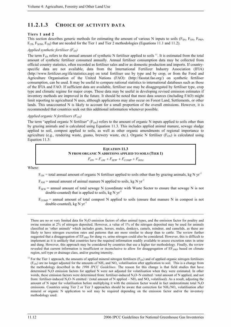
Applied organic N fertilisers (FON) The term “applied organic N fertiliser” (FON) refers to the amount of organic N inputs applied to soils other than by grazing animals and is calculated using Equation 11.3. This includes applied animal manure, sewage sludge applied to soil, compost applied to soils, as well as other organic amendments of regional importance to agriculture (e.g., rendering waste, guano, brewery waste, etc.). Organic N fertiliser (FON) is calculated using Equation 11.3:
EQUATION 11.3 N FROM ORGANIC N ADDITIONS APPLIED TO SOILS (TIER 1)
OOACOMPSEWAMON FFFFF +++=
Where:
FON = total annual amount of organic N fertiliser applied to soils other than by grazing animals, kg N yr-1
FAM = annual amount of animal manure N applied to soils, kg N yr-1
FSEW = annual amount of total sewage N (coordinate with Waste Sector to ensure that sewage N is not double-counted) that is applied to soils, kg N yr-1
FCOMP = annual amount of total compost N applied to soils (ensure that manure N in compost is not double-counted), kg N yr-1
There are no or very limited data for N2O emission factors of other animal types, and the emission factor for poultry and swine remains at 2% of nitrogen deposited. However, a value of 1% of the nitrogen deposited may be used for animals classified as ‘other animals’ which includes goats, horses, mules, donkeys, camels, reindeer, and camelids, as these are likely to have nitrogen excretion rates and patterns that are more similar to sheep than to cattle. The review further suggested that a disaggregation of EF3PRP for dung vs. urine nitrogen could also be considered. However, this is difficult to implement as it is unlikely that countries have the required information readily available to assess excretion rates in urine and dung. However, this approach may be considered by countries that use a higher tier methodology. Finally, the review revealed that current information is insufficient or inconclusive to allow for disaggregation of EF3PRP based on climate region, soil type or drainage class, and/or grazing intensity.
11 For the Tier 1 approach, the amounts of applied mineral nitrogen fertilisers (FSN) and of applied organic nitrogen fertilisers (FON) are no longer adjusted for the amounts of NH3 and NOx volatilisation after application to soil. This is a change from the methodology described in the 1996 IPCC Guidelines. The reason for this change is that field studies that have determined N2O emission factors for applied N were not adjusted for volatilisation when they were estimated. In other words, these emission factors were determined from: fertiliser-induced N2O–N emitted / total amount of N applied, and not from: fertiliser-induced N2O–N emitted / (total amount of N applied – NH3 and NOx volatilised). As a result, adjusting the amount of N input for volatilisation before multiplying it with the emission factor would in fact underestimate total N2O emissions. Countries using Tier 2 or Tier 3 approaches should be aware that correction for NH3/NOx volatilisation after mineral or organic N application to soil may be required depending on the emission factor and/or the inventory methodology used.
Chapter 11: N2O Emissions from Managed Soils, and CO2 Emissions from Lime and Urea Application
2006 IPCC Guidelines for National Greenhouse Gas Inventories 11.13
FOOA = annual amount of other organic amendments used as fertiliser (e.g., rendering waste, guano, brewery waste, etc.), kg N yr-1
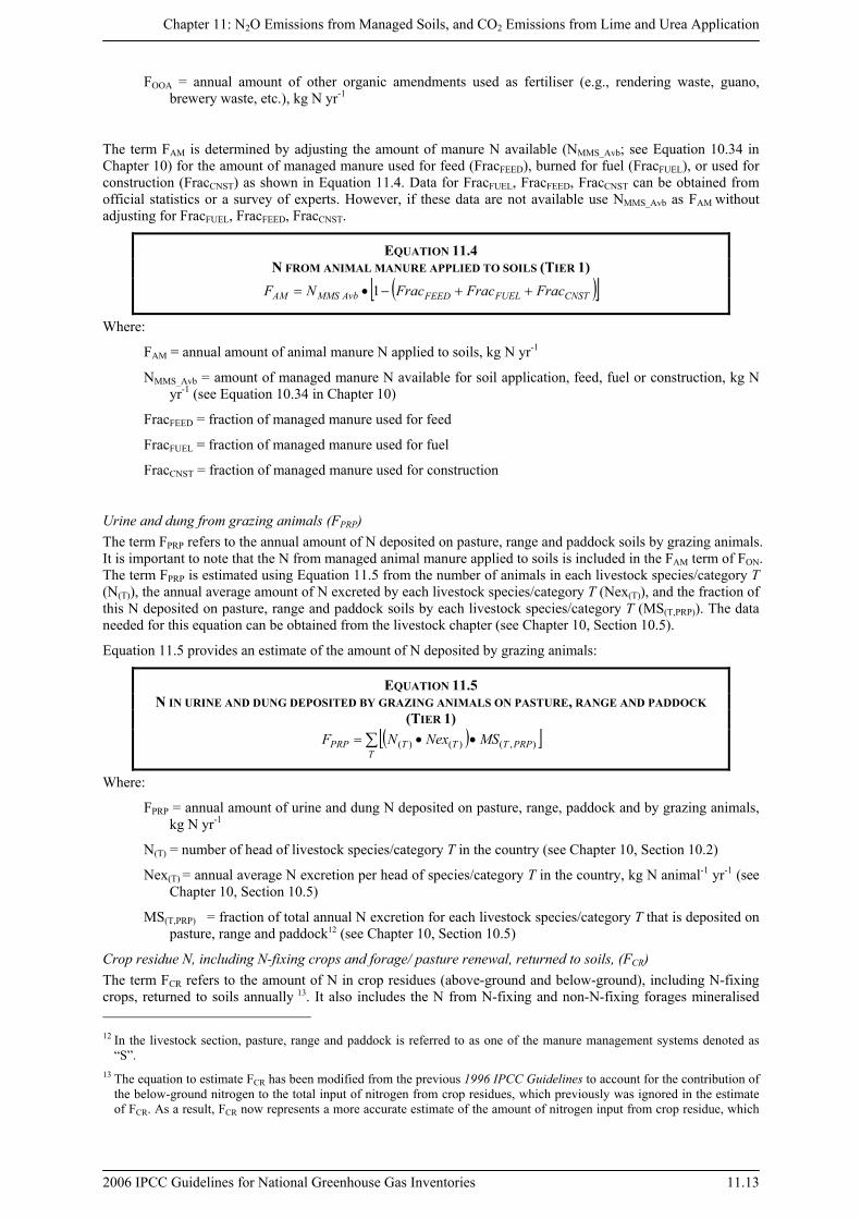
The term FAM is determined by adjusting the amount of manure N available (NMMS_Avb; see Equation 10.34 in Chapter 10) for the amount of managed manure used for feed (FracFEED), burned for fuel (FracFUEL), or used for construction (FracCNST) as shown in Equation 11.4. Data for FracFUEL, FracFEED, FracCNST can be obtained from official statistics or a survey of experts. However, if these data are not available use NMMS_Avb as FAM without adjusting for FracFUEL, FracFEED, FracCNST.
EQUATION 11.4 N FROM ANIMAL MANURE APPLIED TO SOILS (TIER 1)
( )[ ]CNSTFUELFEEDAvbMMSAM FracFracFracNF ++−•= 1
Where:
FAM = annual amount of animal manure N applied to soils, kg N yr-1
NMMS_Avb = amount of managed manure N available for soil application, feed, fuel or construction, kg N yr-1 (see Equation 10.34 in Chapter 10)
FracFEED = fraction of managed manure used for feed
FracFUEL = fraction of managed manure used for fuel
FracCNST = fraction of managed manure used for construction
Urine and dung from grazing animals (FPRP) The term FPRP refers to the annual amount of N deposited on pasture, range and paddock soils by grazing animals. It is important to note that the N from managed animal manure applied to soils is included in the FAM term of FON. The term FPRP is estimated using Equation 11.5 from the number of animals in each livestock species/category T (N(T)), the annual average amount of N excreted by each livestock species/category T (Nex(T)), and the fraction of this N deposited on pasture, range and paddock soils by each livestock species/category T (MS(T,PRP)). The data needed for this equation can be obtained from the livestock chapter (see Chapter 10, Section 10.5).
Equation 11.5 provides an estimate of the amount of N deposited by grazing animals:
EQUATION 11.5 N IN URINE AND DUNG DEPOSITED BY GRAZING ANIMALS ON PASTURE, RANGE AND PADDOCK
(TIER 1) ( )[ ]∑ ••=
TPRPTTTPRP MSNexNF ),()()(
Where:
FPRP = annual amount of urine and dung N deposited on pasture, range, paddock and by grazing animals, kg N yr-1
N(T) = number of head of livestock species/category T in the country (see Chapter 10, Section 10.2)
Nex(T) = annual average N excretion per head of species/category T in the country, kg N animal-1 yr-1 (see Chapter 10, Section 10.5)
MS(T,PRP) = fraction of total annual N excretion for each livestock species/category T that is deposited on pasture, range and paddock12 (see Chapter 10, Section 10.5)
Crop residue N, including N-fixing crops and forage/ pasture renewal, returned to soils, (FCR) The term FCR refers to the amount of N in crop residues (above-ground and below-ground), including N-fixing crops, returned to soils annually 13. It also includes the N from N-fixing and non-N-fixing forages mineralised 12 In the livestock section, pasture, range and paddock is referred to as one of the manure management systems denoted as
“S”. 13 The equation to estimate FCR has been modified from the previous 1996 IPCC Guidelines to account for the contribution of
the below-ground nitrogen to the total input of nitrogen from crop residues, which previously was ignored in the estimate of FCR. As a result, FCR now represents a more accurate estimate of the amount of nitrogen input from crop residue, which
Volume 4: Agriculture, Forestry and Other Land Use
11.14 2006 IPCC Guidelines for National Greenhouse Gas Inventories
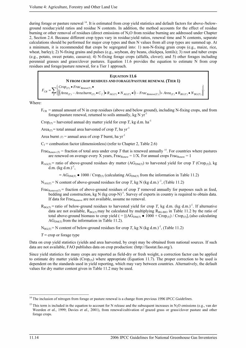
during forage or pasture renewal 14. It is estimated from crop yield statistics and default factors for above-/below-ground residue:yield ratios and residue N contents. In addition, the method accounts for the effect of residue burning or other removal of residues (direct emissions of N2O from residue burning are addressed under Chapter 2, Section 2.4. Because different crop types vary in residue:yield ratios, renewal time and N contents, separate calculations should be performed for major crop types and then N values from all crop types are summed up. At a minimum, it is recommended that crops be segregated into: 1) non-N-fixing grain crops (e.g., maize, rice, wheat, barley); 2) N-fixing grains and pulses (e.g., soybean, dry beans, chickpea, lentils); 3) root and tuber crops (e.g., potato, sweet potato, cassava); 4) N-fixing forage crops (alfalfa, clover); and 5) other forages including perennial grasses and grass/clover pastures. Equation 11.6 provides the equation to estimate N from crop residues and forage/pasture renewal, for a Tier 1 approach.
EQUATION 11.6 N FROM CROP RESIDUES AND FORAGE/PASTURE RENEWAL (TIER 1)
T TBGTBGTTmoveReTAGTAGfTT
TnewReTCR NRAreaFracNRCburntAreaArea
FracCropF
)()()()()()()()(
)()(
1
Where:
FCR = annual amount of N in crop residues (above and below ground), including N-fixing crops, and from forage/pasture renewal, returned to soils annually, kg N yr-1
Crop(T) = harvested annual dry matter yield for crop T, kg d.m. ha-1
Area(T) = total annual area harvested of crop T, ha yr-1
Area burnt (T) = annual area of crop T burnt, ha yr-1
Cf = combustion factor (dimensionless) (refer to Chapter 2, Table 2.6)
FracRenew (T) = fraction of total area under crop T that is renewed annually 15. For countries where pastures are renewed on average every X years, FracRenew = 1/X. For annual crops FracRenew = 1
RAG(T) = ratio of above-ground residues dry matter (AGDM(T)) to harvested yield for crop T (Crop(T)), kg d.m. (kg d.m.)-1,
= AGDM(T) ● 1000 / Crop(T) (calculating AGDM(T) from the information in Table 11.2)
NAG(T) = N content of above-ground residues for crop T, kg N (kg d.m.) -1, (Table 11.2)
FracRemove(T) = fraction of above-ground residues of crop T removed annually for purposes such as feed, bedding and construction, kg N (kg crop-N)-1. Survey of experts in country is required to obtain data. If data for FracRemove are not available, assume no removal.
RBG(T) = ratio of below-ground residues to harvested yield for crop T, kg d.m. (kg d.m.)-1. If alternative data are not available, RBG(T) may be calculated by multiplying RBG-BIO in Table 11.2 by the ratio of total above-ground biomass to crop yield ( = [(AGDM(T) ● 1000 + Crop(T)) / Crop(T)], (also calculating AGDM(T) from the information in Table 11.2).
NBG(T) = N content of below-ground residues for crop T, kg N (kg d.m.)-1, (Table 11.2)
T = crop or forage type
Data on crop yield statistics (yields and area harvested, by crop) may be obtained from national sources. If such data are not available, FAO publishes data on crop production: (http://faostat.fao.org/).
Since yield statistics for many crops are reported as field-dry or fresh weight, a correction factor can be applied to estimate dry matter yields (Crop(T)) where appropriate (Equation 11.7). The proper correction to be used is dependent on the standards used in yield reporting, which may vary between countries. Alternatively, the default values for dry matter content given in Table 11.2 may be used.
14 The inclusion of nitrogen from forage or pasture renewal is a change from previous 1996 IPCC Guidelines. 15 This term is included in the equation to account for N release and the subsequent increases in N2O emissions (e.g., van der
Weerden et al., 1999; Davies et al., 2001), from renewal/cultivation of grazed grass or grass/clover pasture and other forage crops.
Chapter 11: N2O Emissions from Managed Soils, and CO2 Emissions from Lime and Urea Application
2006 IPCC Guidelines for National Greenhouse Gas Inventories 11.15
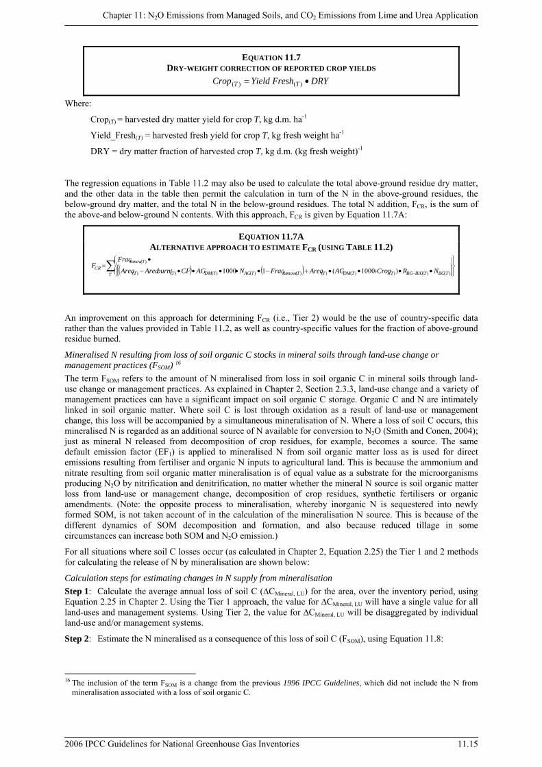
EQUATION 11.7 DRY-WEIGHT CORRECTION OF REPORTED CROP YIELDS
DRYFreshYieldCrop TT )()(
Where:
Crop(T) = harvested dry matter yield for crop T, kg d.m. ha-1
Yield_Fresh(T) = harvested fresh yield for crop T, kg fresh weight ha-1
DRY = dry matter fraction of harvested crop T, kg d.m. (kg fresh weight)-1
The regression equations in Table 11.2 may also be used to calculate the total above-ground residue dry matter, and the other data in the table then permit the calculation in turn of the N in the above-ground residues, the below-ground dry matter, and the total N in the below-ground residues. The total N addition, FCR, is the sum of the above-and below-ground N contents. With this approach, FCR is given by Equation 11.7A:
EQUATION 11.7A ALTERNATIVE APPROACH TO ESTIMATE FCR (USING TABLE 11.2)
T TBGTBIOBGTTDMTTmoveReTAGTDMTT
TnewReCR NRCropAGAreaFracNAGCFburntAreaArea
FracF
)()()()()()()()()()(
)(
)1000(11000
An improvement on this approach for determining FCR (i.e., Tier 2) would be the use of country-specific data rather than the values provided in Table 11.2, as well as country-specific values for the fraction of above-ground residue burned.
Mineralised N resulting from loss of soil organic C stocks in mineral soils through land-use change or management practices (FSOM) 16
The term FSOM refers to the amount of N mineralised from loss in soil organic C in mineral soils through land-use change or management practices. As explained in Chapter 2, Section 2.3.3, land-use change and a variety of management practices can have a significant impact on soil organic C storage. Organic C and N are intimately linked in soil organic matter. Where soil C is lost through oxidation as a result of land-use or management change, this loss will be accompanied by a simultaneous mineralisation of N. Where a loss of soil C occurs, this mineralised N is regarded as an additional source of N available for conversion to N2O (Smith and Conen, 2004); just as mineral N released from decomposition of crop residues, for example, becomes a source. The same default emission factor (EF1) is applied to mineralised N from soil organic matter loss as is used for direct emissions resulting from fertiliser and organic N inputs to agricultural land. This is because the ammonium and nitrate resulting from soil organic matter mineralisation is of equal value as a substrate for the microorganisms producing N2O by nitrification and denitrification, no matter whether the mineral N source is soil organic matter loss from land-use or management change, decomposition of crop residues, synthetic fertilisers or organic amendments. (Note: the opposite process to mineralisation, whereby inorganic N is sequestered into newly formed SOM, is not taken account of in the calculation of the mineralisation N source. This is because of the different dynamics of SOM decomposition and formation, and also because reduced tillage in some circumstances can increase both SOM and N2O emission.)
For all situations where soil C losses occur (as calculated in Chapter 2, Equation 2.25) the Tier 1 and 2 methods for calculating the release of N by mineralisation are shown below:
Calculation steps for estimating changes in N supply from mineralisation
Step 1: Calculate the average annual loss of soil C (∆CMineral, LU) for the area, over the inventory period, using Equation 2.25 in Chapter 2. Using the Tier 1 approach, the value for ∆CMineral, LU will have a single value for all land-uses and management systems. Using Tier 2, the value for ∆CMineral, LU will be disaggregated by individual land-use and/or management systems.
Step 2: Estimate the N mineralised as a consequence of this loss of soil C (FSOM), using Equation 11.8:
16 The inclusion of the term FSOM is a change from the previous 1996 IPCC Guidelines, which did not include the N from
mineralisation associated with a loss of soil organic C.
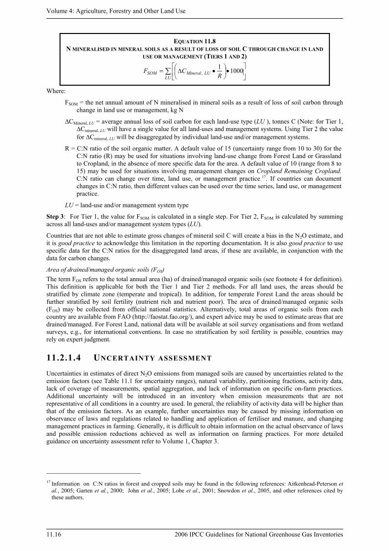
Volume 4: Agriculture, Forestry and Other Land Use
11.16 2006 IPCC Guidelines for National Greenhouse Gas Inventories
EQUATION 11.8 N MINERALISED IN MINERAL SOILS AS A RESULT OF LOSS OF SOIL C THROUGH CHANGE IN LAND
USE OR MANAGEMENT (TIERS 1 AND 2)
∑ ⎥⎦
⎤⎢⎣
⎡•⎟
⎠⎞
⎜⎝⎛ •Δ=
LULUeralMinSOM R
CF 10001,
Where:
FSOM = the net annual amount of N mineralised in mineral soils as a result of loss of soil carbon through change in land use or management, kg N
∆CMineral, LU = average annual loss of soil carbon for each land-use type (LU ), tonnes C (Note: for Tier 1, ∆Cmineral, LU will have a single value for all land-uses and management systems. Using Tier 2 the value for ΔCmineral, LU will be disaggregated by individual land-use and/or management systems.
R = C:N ratio of the soil organic matter. A default value of 15 (uncertainty range from 10 to 30) for the C:N ratio (R) may be used for situations involving land-use change from Forest Land or Grassland to Cropland, in the absence of more specific data for the area. A default value of 10 (range from 8 to 15) may be used for situations involving management changes on Cropland Remaining Cropland. C:N ratio can change over time, land use, or management practice 17. If countries can document changes in C:N ratio, then different values can be used over the time series, land use, or management practice.
LU = land-use and/or management system type
Step 3: For Tier 1, the value for FSOM is calculated in a single step. For Tier 2, FSOM is calculated by summing across all land-uses and/or management system types (LU).
Countries that are not able to estimate gross changes of mineral soil C will create a bias in the N2O estimate, and it is good practice to acknowledge this limitation in the reporting documentation. It is also good practice to use specific data for the C:N ratios for the disaggregated land areas, if these are available, in conjunction with the data for carbon changes.
Area of drained/managed organic soils (FOS) The term FOS refers to the total annual area (ha) of drained/managed organic soils (see footnote 4 for definition). This definition is applicable for both the Tier 1 and Tier 2 methods. For all land uses, the areas should be stratified by climate zone (temperate and tropical). In addition, for temperate Forest Land the areas should be further stratified by soil fertility (nutrient rich and nutrient poor). The area of drained/managed organic soils (FOS) may be collected from official national statistics. Alternatively, total areas of organic soils from each country are available from FAO (http://faostat.fao.org/), and expert advice may be used to estimate areas that are drained/managed. For Forest Land, national data will be available at soil survey organisations and from wetland surveys, e.g., for international conventions. In case no stratification by soil fertility is possible, countries may rely on expert judgment.
11.2.1.4 UNCERTAINTY ASSESSMENT Uncertainties in estimates of direct N2O emissions from managed soils are caused by uncertainties related to the emission factors (see Table 11.1 for uncertainty ranges), natural variability, partitioning fractions, activity data, lack of coverage of measurements, spatial aggregation, and lack of information on specific on-farm practices. Additional uncertainty will be introduced in an inventory when emission measurements that are not representative of all conditions in a country are used. In general, the reliability of activity data will be higher than that of the emission factors. As an example, further uncertainties may be caused by missing information on observance of laws and regulations related to handling and application of fertiliser and manure, and changing management practices in farming. Generally, it is difficult to obtain information on the actual observance of laws and possible emission reductions achieved as well as information on farming practices. For more detailed guidance on uncertainty assessment refer to Volume 1, Chapter 3.
17 Information on C:N ratios in forest and cropped soils may be found in the following references: Aitkenhead-Peterson et
al., 2005; Garten et al., 2000; John et al., 2005; Lobe et al., 2001; Snowdon et al., 2005, and other references cited by these authors.
Chapter 11: N2O Emissions from Managed Soils, and CO2 Emissions from Lime and Urea Application
2006 IPCC Guidelines for National Greenhouse Gas Inventories 11.17
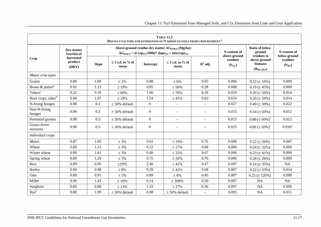
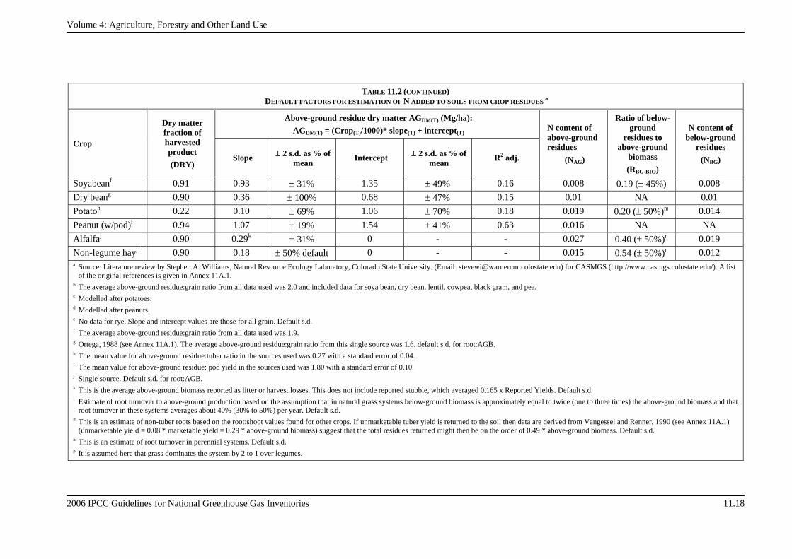
TABLE 11.2 DEFAULT FACTORS FOR ESTIMATION OF N ADDED TO SOILS FROM CROP RESIDUES a
Crop
Dry matter fraction of harvested product (DRY)
Above-ground residue dry matter AGDM(T) (Mg/ha): AGDM(T) = (Crop(T)/1000)* slope(T) + intercept(T) N content of
above-ground residues
(NAG)
Ratio of below-ground
residues to above-ground
biomass (RBG-BIO)
N content of below-ground
residues (NBG) Slope 2 s.d. as % of
mean Intercept 2 s.d. as % of mean R2 adj.
Major crop types
Grains 0.88 1.09 2% 0.88 6% 0.65 0.006 0.22 ( 16%) 0.009 Beans & pulsesb 0.91 1.13 19% 0.85 56% 0.28 0.008 0.19 ( 45%) 0.008 Tubersc 0.22 0.10 69% 1.06 70% 0.18 0.019 0.20 ( 50%) 0.014 Root crops, otherd 0.94 1.07 19% 1.54 41% 0.63 0.016 0.20 ( 50%) 0.014 N-fixing forages 0.90 0.3 50% default 0 - - 0.027 0.40 ( 50%) 0.022 Non-N-fixing forages 0.90 0.3 50% default 0 - - 0.015 0.54 ( 50%) 0.012
Perennial grasses 0.90 0.3 50% default 0 - - 0.015 0.80 ( 50%)l 0.012 Grass-clover mixtures 0.90 0.3 50% default 0 - - 0.025 0.80 ( 50%)l 0.016p
Individual crops
Maize 0.87 1.03 3% 0.61 19% 0.76 0.006 0.22 ( 26%) 0.007 Wheat 0.89 1.51 3% 0.52 17% 0.68 0.006 0.24 ( 32%) 0.009 Winter wheat 0.89 1.61 3% 0.40 25% 0.67 0.006 0.23 ( 41%) 0.009 Spring wheat 0.89 1.29 5% 0.75 26% 0.76 0.006 0.28 ( 26%) 0.009 Rice 0.89 0.95 19% 2.46 41% 0.47 0.007 0.16 ( 35%) NA Barley 0.89 0.98 8% 0.59 41% 0.68 0.007 0.22 ( 33%) 0.014 Oats 0.89 0.91 5% 0.89 8% 0.45 0.007 0.25 ( 120%) 0.008 Millet 0.90 1.43 18% 0.14 308% 0.50 0.007 NA NA Sorghum 0.89 0.88 13% 1.33 27% 0.36 0.007 NA 0.006 Ryee 0.88 1.09 50% default 0.88 50% default - 0.005 NA 0.011
Volume 4: Agriculture, Forestry and Other Land Use
2006 IPCC Guidelines for National Greenhouse Gas Inventories 11.18
TABLE 11.2 (CONTINUED) DEFAULT FACTORS FOR ESTIMATION OF N ADDED TO SOILS FROM CROP RESIDUES a
Crop
Dry matter fraction of harvested product (DRY)
Above-ground residue dry matter AGDM(T) (Mg/ha): AGDM(T) = (Crop(T)/1000)* slope(T) + intercept(T) N content of
above-ground residues
(NAG)
Ratio of below-ground
residues to above-ground
biomass (RBG-BIO)
N content of below-ground
residues (NBG) Slope 2 s.d. as % of
mean Intercept 2 s.d. as % of mean R2 adj.
Soyabeanf 0.91 0.93 31% 1.35 49% 0.16 0.008 0.19 ( 45%) 0.008 Dry beang 0.90 0.36 100% 0.68 47% 0.15 0.01 NA 0.01 Potatoh 0.22 0.10 69% 1.06 70% 0.18 0.019 0.20 ( 50%)m 0.014 Peanut (w/pod)i 0.94 1.07 19% 1.54 41% 0.63 0.016 NA NA Alfalfaj 0.90 0.29k 31% 0 - - 0.027 0.40 ( 50%)n 0.019 Non-legume hayj 0.90 0.18 50% default 0 - - 0.015 0.54 ( 50%)n 0.012 a Source: Literature review by Stephen A. Williams, Natural Resource Ecology Laboratory, Colorado State University. (Email: [email protected]) for CASMGS (http://www.casmgs.colostate.edu/). A list
of the original references is given in Annex 11A.1. b The average above-ground residue:grain ratio from all data used was 2.0 and included data for soya bean, dry bean, lentil, cowpea, black gram, and pea. c Modelled after potatoes. d Modelled after peanuts. e No data for rye. Slope and intercept values are those for all grain. Default s.d. f The average above-ground residue:grain ratio from all data used was 1.9. g Ortega, 1988 (see Annex 11A.1). The average above-ground residue:grain ratio from this single source was 1.6. default s.d. for root:AGB. h The mean value for above-ground residue:tuber ratio in the sources used was 0.27 with a standard error of 0.04. I The mean value for above-ground residue: pod yield in the sources used was 1.80 with a standard error of 0.10. j Single source. Default s.d. for root:AGB. k This is the average above-ground biomass reported as litter or harvest losses. This does not include reported stubble, which averaged 0.165 x Reported Yields. Default s.d. l Estimate of root turnover to above-ground production based on the assumption that in natural grass systems below-ground biomass is approximately equal to twice (one to three times) the above-ground biomass and that
root turnover in these systems averages about 40% (30% to 50%) per year. Default s.d. m This is an estimate of non-tuber roots based on the root:shoot values found for other crops. If unmarketable tuber yield is returned to the soil then data are derived from Vangessel and Renner, 1990 (see Annex 11A.1)
(unmarketable yield = 0.08 * marketable yield = 0.29 * above-ground biomass) suggest that the total residues returned might then be on the order of 0.49 * above-ground biomass. Default s.d. n This is an estimate of root turnover in perennial systems. Default s.d. p It is assumed here that grass dominates the system by 2 to 1 over legumes.
Chapter 11: N2O Emissions from Managed Soils, and CO2 Emissions from Lime and Urea Application
2006 IPCC Guidelines for National Greenhouse Gas Inventories 11.19
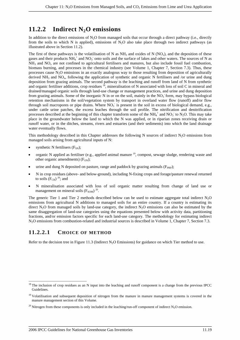
11.2.2 Indirect N2O emissions In addition to the direct emissions of N2O from managed soils that occur through a direct pathway (i.e., directly from the soils to which N is applied), emissions of N2O also take place through two indirect pathways (as illustrated above in Section 11.2).
The first of these pathways is the volatilisation of N as NH3 and oxides of N (NOx), and the deposition of these gases and their products NH4
+ and NO3- onto soils and the surface of lakes and other waters. The sources of N as
NH3 and NOx are not confined to agricultural fertilisers and manures, but also include fossil fuel combustion, biomass burning, and processes in the chemical industry (see Volume 1, Chapter 7, Section 7.3). Thus, these processes cause N2O emissions in an exactly analogous way to those resulting from deposition of agriculturally derived NH3 and NOx, following the application of synthetic and organic N fertilisers and /or urine and dung deposition from grazing animals. The second pathway is the leaching and runoff from land of N from synthetic and organic fertiliser additions, crop residues 18, mineralisation of N associated with loss of soil C in mineral and drained/managed organic soils through land-use change or management practices, and urine and dung deposition from grazing animals. Some of the inorganic N in or on the soil, mainly in the NO3
- form, may bypass biological retention mechanisms in the soil/vegetation system by transport in overland water flow (runoff) and/or flow through soil macropores or pipe drains. Where NO3
- is present in the soil in excess of biological demand, e.g., under cattle urine patches, the excess leaches through the soil profile. The nitrification and denitrification processes described at the beginning of this chapter transform some of the NH4
+ and NO3- to N2O. This may take
place in the groundwater below the land to which the N was applied, or in riparian zones receiving drain or runoff water, or in the ditches, streams, rivers and estuaries (and their sediments) into which the land drainage water eventually flows.
This methodology described in this Chapter addresses the following N sources of indirect N2O emissions from managed soils arising from agricultural inputs of N:
synthetic N fertilisers (FSN);
organic N applied as fertiliser (e.g., applied animal manure 19, compost, sewage sludge, rendering waste and other organic amendments) (FON);
urine and dung N deposited on pasture, range and paddock by grazing animals (FPRP);
N in crop residues (above- and below-ground), including N-fixing crops and forage/pasture renewal returned to soils (FCR) 20; and
N mineralisation associated with loss of soil organic matter resulting from change of land use or management on mineral soils (FSOM) 20.
The generic Tier 1 and Tier 2 methods described below can be used to estimate aggregate total indirect N2O emissions from agricultural N additions to managed soils for an entire country. If a country is estimating its direct N2O from managed soils by land-use category, the indirect N2O emissions can also be estimated by the same disaggregation of land-use categories using the equations presented below with activity data, partitioning fractions, and/or emission factors specific for each land-use category. The methodology for estimating indirect N2O emissions from combustion-related and industrial sources is described in Volume 1, Chapter 7, Section 7.3.
11.2.2.1 CHOICE OF METHOD Refer to the decision tree in Figure 11.3 (Indirect N2O Emissions) for guidance on which Tier method to use.
18 The inclusion of crop residues as an N input into the leaching and runoff component is a change from the previous IPCC
Guidelines. 19 Volatilisation and subsequent deposition of nitrogen from the manure in manure management systems is covered in the
manure management section of this Volume. 20 Nitrogen from these components is only included in the leaching/run-off component of indirect N2O emission.
Volume 4: Agriculture, Forestry and Other Land Use
11.20 2006 IPCC Guidelines for National Greenhouse Gas Inventories
Figure 11.3 Decision tree for indirect N2O emissions from managed soils
Start
Foreach N source,
do you have rigorouslydocumented country-specific
emission factors (EF4 or EF5) and as appropriate rigorously documented
country-specific partitioning fractions (FracGASF,FracGASM, FracLEACH)
values?
Obtain country-specific data.
Estimate emissions using the Tier 1equation with default emission
and partitioning factors andavailable activity data.
Note:1: N sources include: synthetic N fertilizer, organic N additions, urine and dung depositions, crop residue, N mineralization/immobilization associated with loss/gain of soil C on mineral soils as a result of land use change or management practices (crop residue and N mineralization/immobilization is only accounted for in the indirect N2O emissions from leaching/runoff). Sewage sludge or other organic N additions can be included if sufficient information is available.2: See Volume 1 Chapter 4, "Methodological Choice and Identification of Key Categories" (noting Section 4.1.2 on limited resources), for discussion of key categories and use of decision trees.3: As a rule of thumb, a sub-source category would be significant if it accounts for 25-30% of emissions from the source category.
Is this akey category2
and is this N source significant3?
No
Yes
Estimate emissions using Tier 2 equation, country-specific activity data and
country-specific emission factors and partitioning fractions, or Tier 3 method.
YesYes
Box 1: Tier 1
Box 2: Tier 2
No
Estimate emissions with Tier 2 equation, using a mix of country-specific and other
available data and country-specificemission and partitioning factors.
For eachagricultural N source1, for both
volatilization and leaching/runoff, ask: Do you have country-specific
activity data?
Box 4: Tier 2 or 3
Do youhave rigorously
documented country-specificEF values (EF4 or EF5) and as
appropriate rigorously documented country-specific partitioning fractions
(FracGASF, FracGASM, FracLEACH)values?
Estimate emissions using Tier 1 or Tier 2equation, country-specific activity data and a mix of county-specific or default
emission factors and partitioning fractions.
No
Yes
Box 3: Tier 1 or 2
No
Chapter 11: N2O Emissions from Managed Soils, and CO2 Emissions from Lime and Urea Application
2006 IPCC Guidelines for National Greenhouse Gas Inventories 11.21
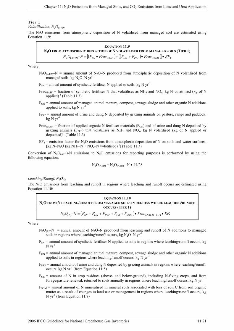
Tier 1 Volatilisation, N2O(ATD) The N2O emissions from atmospheric deposition of N volatilised from managed soil are estimated using Equation 11.9:
EQUATION 11.9 N2O FROM ATMOSPHERIC DEPOSITION OF N VOLATILISED FROM MANAGED SOILS (TIER 1)
( ) ( )( )[ ] 4)(2 EFFracFFFracFNON GASMPRPONGASFSNATD ••++•=−
Where:
N2O(ATD)–N = annual amount of N2O–N produced from atmospheric deposition of N volatilised from managed soils, kg N2O–N yr-1
FSN = annual amount of synthetic fertiliser N applied to soils, kg N yr-1
FracGASF = fraction of synthetic fertiliser N that volatilises as NH3 and NOx, kg N volatilised (kg of N applied)-1 (Table 11.3)
FON = annual amount of managed animal manure, compost, sewage sludge and other organic N additions applied to soils, kg N yr-1
FPRP = annual amount of urine and dung N deposited by grazing animals on pasture, range and paddock, kg N yr-1
FracGASM = fraction of applied organic N fertiliser materials (FON) and of urine and dung N deposited by grazing animals (FPRP) that volatilises as NH3 and NOx, kg N volatilised (kg of N applied or deposited)-1 (Table 11.3)
EF4 = emission factor for N2O emissions from atmospheric deposition of N on soils and water surfaces, [kg N–N2O (kg NH3–N + NOx–N volatilised)-1] (Table 11.3)
Conversion of N2O(ATD)-N emissions to N2O emissions for reporting purposes is performed by using the following equation:
N2O(ATD) = N2O(ATD) –N • 44/28
Leaching/Runoff, N2O(L) The N2O emissions from leaching and runoff in regions where leaching and runoff occurs are estimated using Equation 11.10:
EQUATION 11.10 N2O FROM N LEACHING/RUNOFF FROM MANAGED SOILS IN REGIONS WHERE LEACHING/RUNOFF
OCCURS (TIER 1) ( ) 5)()(2 EFFracFFFFFNON HLEACHSOMCRPRPONSNL ••++++=− −
Where:
N2O(L)–N = annual amount of N2O–N produced from leaching and runoff of N additions to managed soils in regions where leaching/runoff occurs, kg N2O–N yr-1
FSN = annual amount of synthetic fertiliser N applied to soils in regions where leaching/runoff occurs, kg N yr-1
FON = annual amount of managed animal manure, compost, sewage sludge and other organic N additions applied to soils in regions where leaching/runoff occurs, kg N yr-1
FPRP = annual amount of urine and dung N deposited by grazing animals in regions where leaching/runoff occurs, kg N yr-1 (from Equation 11.5)
FCR = amount of N in crop residues (above- and below-ground), including N-fixing crops, and from forage/pasture renewal, returned to soils annually in regions where leaching/runoff occurs, kg N yr-1
FSOM = annual amount of N mineralised in mineral soils associated with loss of soil C from soil organic matter as a result of changes to land use or management in regions where leaching/runoff occurs, kg N yr-1 (from Equation 11.8)
Volume 4: Agriculture, Forestry and Other Land Use
11.22 2006 IPCC Guidelines for National Greenhouse Gas Inventories
FracLEACH-(H) = fraction of all N added to/mineralised in managed soils in regions where leaching/runoff occurs that is lost through leaching and runoff, kg N (kg of N additions)-1 (Table 11.3)
EF5 = emission factor for N2O emissions from N leaching and runoff, kg N2O–N (kg N leached and runoff)-1 (Table 11.3)
Note: If a country is able to estimate the quantity of N mineralised from organic soils, then include this as an additional input to Equation 11.10.
Conversion of N2O(L)–N emissions to N2O emissions for reporting purposes is performed by using the following equation:
N2O(L) = N2O(L)–N • 44/28
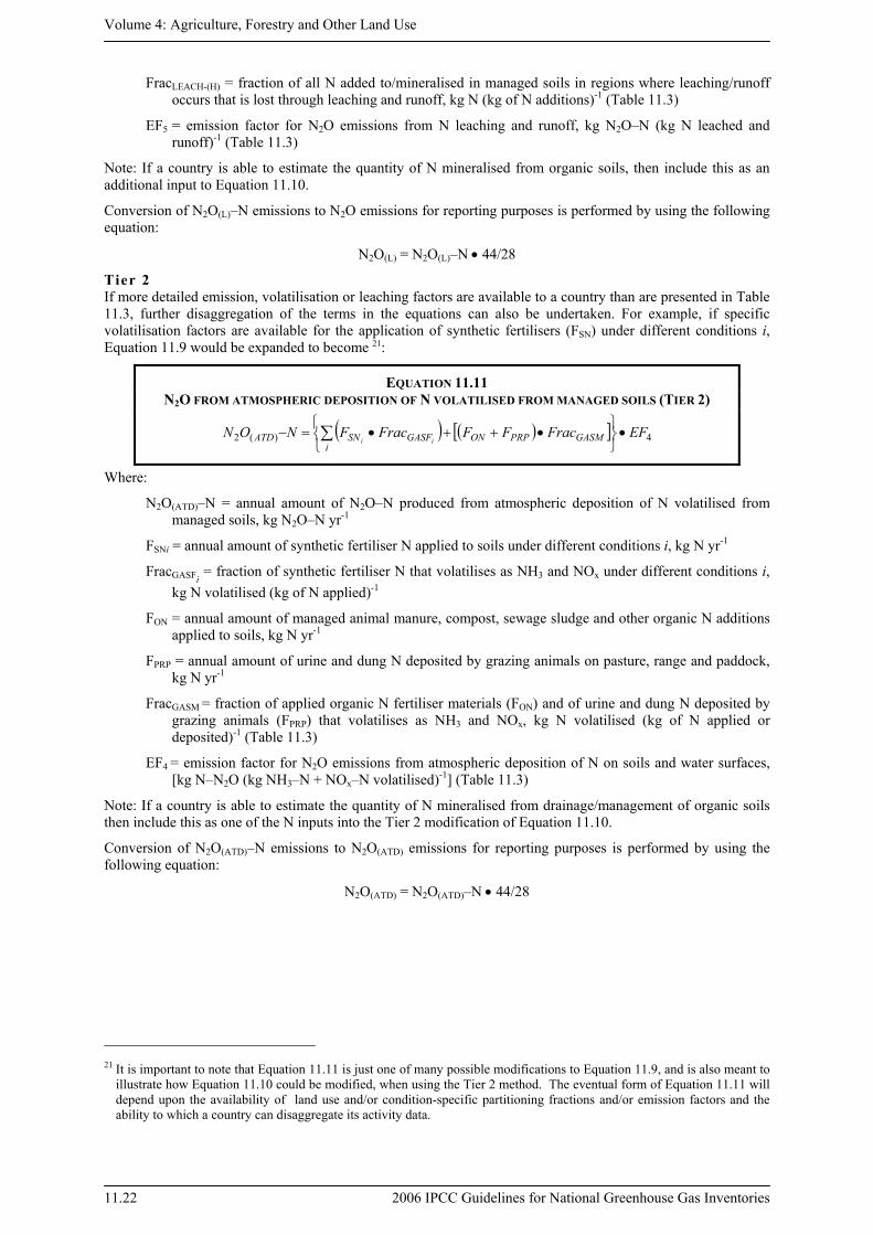
Tier 2 If more detailed emission, volatilisation or leaching factors are available to a country than are presented in Table 11.3, further disaggregation of the terms in the equations can also be undertaken. For example, if specific volatilisation factors are available for the application of synthetic fertilisers (FSN) under different conditions i, Equation 11.9 would be expanded to become 21:
EQUATION 11.11 N2O FROM ATMOSPHERIC DEPOSITION OF N VOLATILISED FROM MANAGED SOILS (TIER 2)
( ) ( )[ ] 4)(2 EFFracFFFracFNON GASMPRPONi
GASFSNATD ii•
⎭⎬⎫
⎩⎨⎧
•++•=− ∑
Where:
N2O(ATD)–N = annual amount of N2O–N produced from atmospheric deposition of N volatilised from managed soils, kg N2O–N yr-1
FSNi = annual amount of synthetic fertiliser N applied to soils under different conditions i, kg N yr-1
FracGASFi = fraction of synthetic fertiliser N that volatilises as NH3 and NOx under different conditions i,
kg N volatilised (kg of N applied)-1
FON = annual amount of managed animal manure, compost, sewage sludge and other organic N additions applied to soils, kg N yr-1
FPRP = annual amount of urine and dung N deposited by grazing animals on pasture, range and paddock, kg N yr-1
FracGASM = fraction of applied organic N fertiliser materials (FON) and of urine and dung N deposited by grazing animals (FPRP) that volatilises as NH3 and NOx, kg N volatilised (kg of N applied or deposited)-1 (Table 11.3)
EF4 = emission factor for N2O emissions from atmospheric deposition of N on soils and water surfaces, [kg N–N2O (kg NH3–N + NOx–N volatilised)-1] (Table 11.3)
Note: If a country is able to estimate the quantity of N mineralised from drainage/management of organic soils then include this as one of the N inputs into the Tier 2 modification of Equation 11.10.
Conversion of N2O(ATD)–N emissions to N2O(ATD) emissions for reporting purposes is performed by using the following equation:
N2O(ATD) = N2O(ATD)–N • 44/28
21 It is important to note that Equation 11.11 is just one of many possible modifications to Equation 11.9, and is also meant to
illustrate how Equation 11.10 could be modified, when using the Tier 2 method. The eventual form of Equation 11.11 will depend upon the availability of land use and/or condition-specific partitioning fractions and/or emission factors and the ability to which a country can disaggregate its activity data.
Chapter 11: N2O Emissions from Managed Soils, and CO2 Emissions from Lime and Urea Application
2006 IPCC Guidelines for National Greenhouse Gas Inventories 11.23
Tier 3 Tier 3 methods are modelling or measurement approaches. Models are useful as they can relate the variables responsible for the emissions to the size of those emissions. These relationships may then be used to predict emissions from whole countries or regions for which experimental measurements are impracticable. For more information refer to Chapter 2, Section 2.5, where guidance is given that provides a sound scientific basis for the development of a Tier 3 Model-based Accounting System.
11.2.2.2 CHOICE OF EMISSION, VOLATILISATION AND LEACHING FACTORS
The method for estimating indirect N2O emissions includes two emission factors: one associated with volatilised and re-deposited N (EF4), and the second associated with N lost through leaching/runoff (EF5). The method also requires values for the fractions of N that are lost through volatilisation (FracGASF and FracGASM) or leaching/runoff (FracLEACH-(H)). The default values of all these factors are presented in Table 11.3.
Note that in the Tier 1 method, for humid regions or in dryland regions where irrigation (other than drip irrigation) is used, the default FracLEACH-(H) is 0.30. For dryland regions, where precipitation is lower than evapotranspiration throughout most of the year and leaching is unlikely to occur, the default FracLEACH is zero. The method of calculating whether FracLEACH-(H) = 0.30 should be applied is given in Table 11.3.
Country-specific values for EF4 should be used with great caution because of the special complexity of transboundary atmospheric transport. Although inventory compilers may have specific measurements of N deposition and associated N2O flux, in many cases the deposited N may not have originated in their country. Similarly, some of the N that volatilises in their country may be transported to and deposited in another country, where different conditions that affect the fraction emitted as N2O may prevail. For these reasons the value of EF4 is very difficult to determine, and the method presented in Volume 1, Chapter 7, Section 7.3 attributes all indirect N2O emissions resulting from inputs to managed soils to the country of origin of the atmospheric NOx and NH3, rather than the country to which the atmospheric N may have been transported.
11.2.2.3 CHOICE OF ACTIVITY DATA In order to estimate indirect N2O emissions from the various N additions to managed soils, the parameters FSN, FON, FPRP, FCR, FSOM need to be estimated.
Applied synthetic fertiliser (FSN) The term FSN refers to the annual amount of synthetic fertiliser N applied to soils. Refer to the activity data section on direct N2O emissions from managed soils (Section 11.2.1.3) and obtain the value for FSN.
Applied organic N fertilisers (FON) The term FON refers to the amount of organic N fertiliser materials intentionally applied to soils. Refer to the activity data section on direct N2O emissions from managed soils (Section 11.2.1.3) and obtain the value for FON.
Urine and dung from grazing animals (FPRP) The term FPRP refers to the amount of N deposited on soil by animals grazing on pasture, range and paddock. Refer to the activity data section on direct N2O emissions from managed soils (Section 11.2.1.3) and obtain the value for FPRP.
Crop residue N, including N from N-fixing crops and forage/pasture renewal, returned to soils (FCR) The term FCR refers to the amount of N in crop residues (above- and below-ground), including N-fixing crops, returned to soils annually. It also includes the N from N-fixing and non-N-fixing forages mineralised during forage/pasture renewal. Refer to the activity data section on direct N2O emissions from managed soils (Section 11.2.1.3) and obtain the value for FCR.
Mineralised N resulting from loss of soil organic C stocks in mineral soils (FSOM) The term FSOM refers to the amount of N mineralised from the loss of soil organic C in mineral soils through land-use change or management practices. Refer to the activity data section on direct N2O emissions from managed soils (Section 11.2.1.3) and obtain the value for FSOM.
Volume 4: Agriculture, Forestry and Other Land Use
11.24 2006 IPCC Guidelines for National Greenhouse Gas Inventories
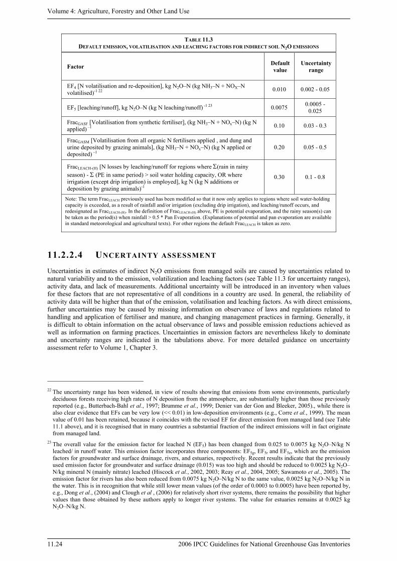
TABLE 11.3 DEFAULT EMISSION, VOLATILISATION AND LEACHING FACTORS FOR INDIRECT SOIL N2O EMISSIONS
Factor Default value
Uncertainty range
EF4 [N volatilisation and re-deposition], kg N2O–N (kg NH3–N + NOX–N volatilised)-1 22 0.010 0.002 - 0.05
EF5 [leaching/runoff], kg N2O–N (kg N leaching/runoff) -1 23 0.0075 0.0005 - 0.025
FracGASF [Volatilisation from synthetic fertiliser], (kg NH3–N + NOx–N) (kg N applied) –1 0.10 0.03 - 0.3
FracGASM [Volatilisation from all organic N fertilisers applied , and dung and urine deposited by grazing animals], (kg NH3–N + NOx–N) (kg N applied or deposited) –1
0.20 0.05 - 0.5
FracLEACH-(H) [N losses by leaching/runoff for regions where Σ(rain in rainy season) - Σ (PE in same period) > soil water holding capacity, OR where irrigation (except drip irrigation) is employed], kg N (kg N additions or deposition by grazing animals)-1
0.30 0.1 - 0.8
Note: The term FracLEACH previously used has been modified so that it now only applies to regions where soil water-holding capacity is exceeded, as a result of rainfall and/or irrigation (excluding drip irrigation), and leaching/runoff occurs, and redesignated as FracLEACH-(H). In the definition of FracLEACH-(H) above, PE is potential evaporation, and the rainy season(s) can be taken as the period(s) when rainfall > 0.5 * Pan Evaporation. (Explanations of potential and pan evaporation are available in standard meteorological and agricultural texts). For other regions the default FracLEACH is taken as zero.
11.2.2.4 UNCERTAINTY ASSESSMENT Uncertainties in estimates of indirect N2O emissions from managed soils are caused by uncertainties related to natural variability and to the emission, volatilization and leaching factors (see Table 11.3 for uncertainty ranges), activity data, and lack of measurements. Additional uncertainty will be introduced in an inventory when values for these factors that are not representative of all conditions in a country are used. In general, the reliability of activity data will be higher than that of the emission, volatilisation and leaching factors. As with direct emissions, further uncertainties may be caused by missing information on observance of laws and regulations related to handling and application of fertiliser and manure, and changing management practices in farming. Generally, it is difficult to obtain information on the actual observance of laws and possible emission reductions achieved as well as information on farming practices. Uncertainties in emission factors are nevertheless likely to dominate and uncertainty ranges are indicated in the tabulations above. For more detailed guidance on uncertainty assessment refer to Volume 1, Chapter 3.
22 The uncertainty range has been widened, in view of results showing that emissions from some environments, particularly
deciduous forests receiving high rates of N deposition from the atmosphere, are substantially higher than those previously reported (e.g., Butterbach-Bahl et al., 1997; Brumme et al., 1999; Denier van der Gon and Bleeker, 2005)., while there is also clear evidence that EFs can be very low (<< 0.01) in low-deposition environments (e.g., Corre et al., 1999). The mean value of 0.01 has been retained, because it coincides with the revised EF for direct emission from managed land (see Table 11.1 above), and it is recognised that in many countries a substantial fraction of the indirect emissions will in fact originate from managed land.
23 The overall value for the emission factor for leached N (EF5) has been changed from 0.025 to 0.0075 kg N2O–N/kg N leached/ in runoff water. This emission factor incorporates three components: EF5g, EF5r and EF5e, which are the emission factors for groundwater and surface drainage, rivers, and estuaries, respectively. Recent results indicate that the previously used emission factor for groundwater and surface drainage (0.015) was too high and should be reduced to 0.0025 kg N2O–N/kg mineral N (mainly nitrate) leached (Hiscock et al., 2002, 2003; Reay et al., 2004, 2005; Sawamoto et al., 2005). The emission factor for rivers has also been reduced from 0.0075 kg N2O–N/kg N to the same value, 0.0025 kg N2O–N/kg N in the water. This is in recognition that while still lower mean values (of the order of 0.0003 to 0.0005) have been reported by, e.g., Dong et al., (2004) and Clough et al , (2006) for relatively short river systems, there remains the possibility that higher values than those obtained by these authors apply to longer river systems. The value for estuaries remains at 0.0025 kg N2O–N/kg N.
Chapter 11: N2O Emissions from Managed Soils, and CO2 Emissions from Lime and Urea Application
2006 IPCC Guidelines for National Greenhouse Gas Inventories 11.25
11.2.3 Completeness, Time series, QA/QC COMPLETENESS Complete coverage of the direct and indirect N2O emissions from managed land requires estimation of emissions for all of the anthropogenic inputs and activities (FSN, FON, FCR, FPRP, FSOM and FOS), if they occur. Experience has shown that none of these sub-categories are likely to be missed in inventories, although countries may have difficulty obtaining accurate statistics for all sub-categories, particularly the amounts of crop residues (by crop type) that are typically returned to soils, and the area of drained/managed organic soils.
Currently, the IPCC method does not explicitly address activities such as plastic sheeting or greenhouse hydroponic systems that may influence N2O emissions. These additional activities can be considered if appropriate, and if national activity data for these activities are collected. Some of these activities can be readily included in national inventories based on available information. For the additional commercial and non-commercial organic fertilisers, the default emission factor used for applied N may be used. Further research will be required to develop the flux data that are needed to develop emission factors for use of plastic sheeting and hydroponic systems in horticultural areas.
DEVELOPING A CONSISTENT TIME SERIES Ideally, the same method is used throughout the entire time series. However, it is likely that the detail and disaggregation of emissions estimates from this source category will improve over time. In cases where some historical data are missing, it may be necessary to derive the data using other references or data sets. For example, annual data of areas for drained/managed organic soils may need to be derived by interpolation from a longer time series based upon long-term trends (e.g., from decadal statistics over a 20- or 30-year period). Estimates of the amounts of crop residue incorporated annually may also need to be derived based on expert judgment.
Interannual changes in FracGASF, FracGASM, FracLEACH, EF4, and EF5 are not expected unless mitigation measures are undertaken. These factors should be changed only with the proper justification and documentation. If updated defaults for any of these variables become available through future research, inventory agencies may recalculate their historical emissions.
It is important that the methods used reflect the results of action taken to reduce emissions and the methods and results are thoroughly documented. If policy measures are implemented such that activity data are affected directly (e.g., increased efficiency of fertiliser use resulting in a decrease in fertiliser consumption), the effect of the policy measures on emissions will be transparent, assuming the activity data are carefully documented. In cases where policy measures have an indirect effect on activity data or emission factors (e.g., a change in animal population feed practices to improve animal productivity that results in a change in N excretion per head), inventory input data should reflect these effects. The inventory text should thoroughly explain the effect of the policies on the input data.
INVENTORY QUALITY ASSURANCE/QUALITY CONTROL (QA/QC) Tier 1 checks of the emission estimates should be undertaken by the persons preparing the inventory along with expert review by people outside the inventory preparation process. Additional Tier 2 quality control checks and quality assurance procedures may also be applicable, particularly if higher tier methods are used to determine direct and indirect N2O emissions from this source category. Supplement the general QA/QC related to data processing, handling, and reporting, with source-specific category procedures discussed below. The persons who collect data are responsible for reviewing the data collection methods, checking the data to ensure that they are collected and aggregated or disaggregated correctly, and cross-checking the data with previous years to ensure that the data are reasonable. The basis for the estimates, whether statistical surveys or ‘desk estimates’, must be reviewed and described as part of the QC effort. Documentation is a crucial component of the review process because it enables reviewers to identify mistakes and suggest improvements.
Review of emission factors The inventory compiler should review the default emission factors and document the rationale for selecting specific values.
If using country-specific factors, the inventory compiler should compare them to the IPCC default emission factors. Also, if accessible, relate to country-specific emission factors used by other countries with comparable circumstances. Differences between country-specific factors and default or other country factors should be explained and documented.
Volume 4: Agriculture, Forestry and Other Land Use
11.26 2006 IPCC Guidelines for National Greenhouse Gas Inventories
Review of any direct measurements If using factors based on direct measurements, the inventory compiler should review the measurements to ensure that they are representative of the actual range of environmental and soil management conditions, and inter-annual climatic variability, and were developed according to recognised standards (IAEA, 1992).
The QA/QC protocol in effect at the sites should also be reviewed and the resulting estimates compared between sites and with default-based estimates.
Activity data check The inventory compiler should compare country-specific data on synthetic fertiliser consumption with fertiliser usage data from the IFA and synthetic fertiliser consumption estimates from the FAO.
The inventory compiler should ensure that N excretion data are consistent with those used for the manure management systems source category.
National crop production statistics should be compared to FAO crop production statistics.
The inventory compiler should ensure that the QA/QC has been completed for livestock characterisation, because data are shared with the livestock section.
Country-specific values for various parameters should be compared to IPCC defaults and any significant differences explained.
External review The inventory compiler should conduct expert (peer) review when first adopting or revising the method. Given the complexity and uniqueness of the parameters used in calculating country-specific factors for these categories, specialists in the field should be involved in such reviews.
REPORTING AND DOCUMENTATION
Direct and Indirect N2O Emissions Document and archive all information required to produce the national emissions inventory estimates. Direct and indirect N2O emissions from managed soils are reported in aggregate or disaggregated by land-use category or other subcategory (e.g., ricelands) under the IPCC category ‘AFOLU’. Reporting should be done at the same level of disaggregation as was done when calculating the emissions. In addition to completing the reporting formats, the following additional information is necessary to document the estimate:
Activity data: Sources of all activity data used in the calculations (i.e., complete citations for the statistical databases from which data were collected), and in cases when activity data were not available directly from databases, the information and assumptions that were used to derive the activity data. This documentation should include the frequency of data collection and estimation, and estimates of accuracy and precision.
Emission factors: The sources of the emission factors that were used (specific IPCC default values or otherwise). In inventories in which country- or region-specific emission factors were used, or in which new methods (other than the default IPCC methods) were used, the scientific basis of these emission factors and methods should be completely described and documented. This includes defining the input parameters and describing the process by which these emission factors and methods are derived, as well as describing sources and magnitudes of uncertainties.
Emission results: Significant fluctuations in emissions between years should be explained. A distinction should be made between changes in activity levels and changes in emission, volatilisation and leaching factors from year to year, and the reasons for these changes documented. If different factors are used for different years, the reasons for this should be explained and documented.
11.3 CO2 EMISSIONS FROM LIMING Liming is used to reduce soil acidity and improve plant growth in managed systems, particularly agricultural lands and managed forests. Adding carbonates to soils in the form of lime (e.g., calcic limestone (CaCO3), or dolomite (CaMg(CO3)2) leads to CO2 emissions as the carbonate limes dissolve and release bicarbonate (2HCO3
-
), which evolves into CO2 and water (H2O).
Inventories can be developed using Tier 1, 2 or 3 approaches, with each successive Tier requiring more detail and resources than the previous one. It is good practice for countries to use higher tiers if CO2 emissions from liming are a key source category.
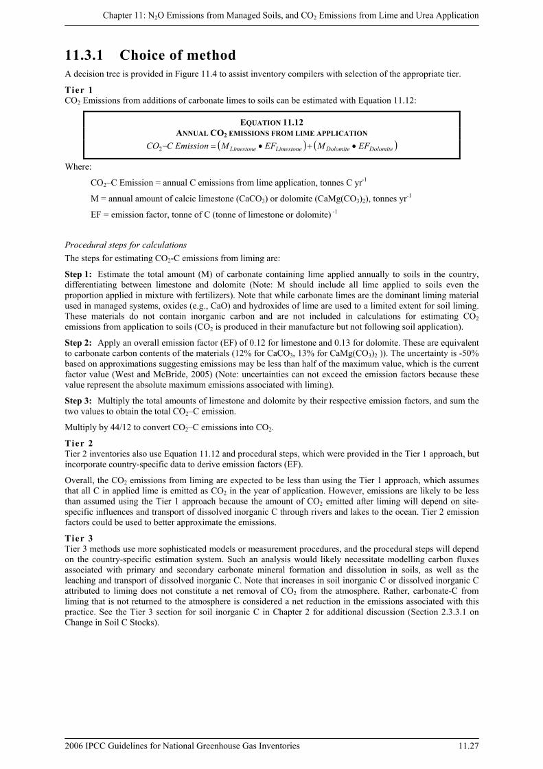
Chapter 11: N2O Emissions from Managed Soils, and CO2 Emissions from Lime and Urea Application
2006 IPCC Guidelines for National Greenhouse Gas Inventories 11.27
11.3.1 Choice of method A decision tree is provided in Figure 11.4 to assist inventory compilers with selection of the appropriate tier.
Tier 1 CO2 Emissions from additions of carbonate limes to soils can be estimated with Equation 11.12:
EQUATION 11.12 ANNUAL CO2 EMISSIONS FROM LIME APPLICATION
( ) ( )DolomiteDolomiteLimestoneLimestone EFMEFMEmissionCCO •+•=−2
Where:
CO2–C Emission = annual C emissions from lime application, tonnes C yr-1
M = annual amount of calcic limestone (CaCO3) or dolomite (CaMg(CO3)2), tonnes yr-1
EF = emission factor, tonne of C (tonne of limestone or dolomite) -1
Procedural steps for calculations The steps for estimating CO2-C emissions from liming are:
Step 1: Estimate the total amount (M) of carbonate containing lime applied annually to soils in the country, differentiating between limestone and dolomite (Note: M should include all lime applied to soils even the proportion applied in mixture with fertilizers). Note that while carbonate limes are the dominant liming material used in managed systems, oxides (e.g., CaO) and hydroxides of lime are used to a limited extent for soil liming. These materials do not contain inorganic carbon and are not included in calculations for estimating CO2 emissions from application to soils (CO2 is produced in their manufacture but not following soil application).
Step 2: Apply an overall emission factor (EF) of 0.12 for limestone and 0.13 for dolomite. These are equivalent to carbonate carbon contents of the materials (12% for CaCO3, 13% for CaMg(CO3)2 )). The uncertainty is -50% based on approximations suggesting emissions may be less than half of the maximum value, which is the current factor value (West and McBride, 2005) (Note: uncertainties can not exceed the emission factors because these value represent the absolute maximum emissions associated with liming).
Step 3: Multiply the total amounts of limestone and dolomite by their respective emission factors, and sum the two values to obtain the total CO2–C emission.
Multiply by 44/12 to convert CO2–C emissions into CO2.
Tier 2 Tier 2 inventories also use Equation 11.12 and procedural steps, which were provided in the Tier 1 approach, but incorporate country-specific data to derive emission factors (EF).
Overall, the CO2 emissions from liming are expected to be less than using the Tier 1 approach, which assumes that all C in applied lime is emitted as CO2 in the year of application. However, emissions are likely to be less than assumed using the Tier 1 approach because the amount of CO2 emitted after liming will depend on site-specific influences and transport of dissolved inorganic C through rivers and lakes to the ocean. Tier 2 emission factors could be used to better approximate the emissions.
Tier 3 Tier 3 methods use more sophisticated models or measurement procedures, and the procedural steps will depend on the country-specific estimation system. Such an analysis would likely necessitate modelling carbon fluxes associated with primary and secondary carbonate mineral formation and dissolution in soils, as well as the leaching and transport of dissolved inorganic C. Note that increases in soil inorganic C or dissolved inorganic C attributed to liming does not constitute a net removal of CO2 from the atmosphere. Rather, carbonate-C from liming that is not returned to the atmosphere is considered a net reduction in the emissions associated with this practice. See the Tier 3 section for soil inorganic C in Chapter 2 for additional discussion (Section 2.3.3.1 on Change in Soil C Stocks).
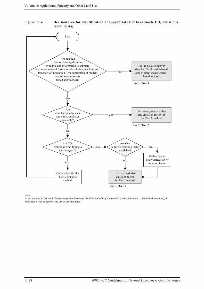
Volume 4: Agriculture, Forestry and Other Land Use
11.28 2006 IPCC Guidelines for National Greenhouse Gas Inventories
Figure 11.4 Decision tree for identification of appropriate tier to estimate CO2 emissions from liming.
Start
Are CO2emissions from liming a
key category1?
Collect data for the Tier 3 or Tier 2
method.
Use country-specific dataand emission factor for
the Tier 2 method.
No
Note:1: See Volume 1 Chapter 4, "Methodological Choice and Identification of Key Categories" (noting Section 4.1.2 on limited resources), for discussion of key categories and use of decision trees.
Arecountry-specific dataand emission factor
available?
Yes
Yes
Use data to derive emission factor
for Tier 1 method.
No
No
Box 2: Tier 2
Box 3: Tier 3
Yes
Use the detailed activitydata for Tier 3 model-basedand/or direct measurement-
based method.
Are detaileddata on lime application
available and information to estimatecarbonate mineral formation/dissolution, leaching and
transport of inorganic C (for application of models and/or measurement-based approaches)?
Are datato derive emission factor
available?
Gather data toallow derivation of
emission factor.Yes
No
Box 1: Tier 1
Chapter 11: N2O Emissions from Managed Soils, and CO2 Emissions from Lime and Urea Application
2006 IPCC Guidelines for National Greenhouse Gas Inventories 11.29
11.3.2 Choice of emission factors Tier 1 Default emission factors (EF) are 0.12 for limestone and 0.13 for dolomite.
Tier 2 Derivation of emission factors using country-specific data could entail differentiation of sources with variable compositions of lime; different carbonate liming materials (limestone as well as other sources such as marl and shell deposits) can vary somewhat in their C content and overall purity. Each material would have a unique emission factor based on the C content.
Country-specific emission factors could also account for the proportion of carbonate-C from liming that is emitted to the atmosphere as CO2 (e.g., West and McBride, 2005). Dissolved inorganic C in soils can form secondary minerals and precipitate with the Ca or Mg that was added during liming. Furthermore, dissolved inorganic C (bicarbonate) can be transported with Ca and Mg through the soil to deep groundwater, lakes and eventually to the ocean (Robertson and Grace, 2004). In either case, the net emission of CO2 to the atmosphere is less than the original amount of C added as lime. Country-specific emission factors can be derived if there are sufficient data and understanding of inorganic carbon transformations, in addition to knowledge about transport of aqueous Ca, Mg, and inorganic C. It is good practice to document the source of information and method used for deriving country-specific values in the reporting process.
Tier 3 Tier 3 approaches are based on estimating variable emissions from year to year, which depends on a variety of site specific characteristics and environmental drivers. No emission factors are directly estimated.
11.3.3 Choice of activity data Tier 1 Optimally, national usage statistics for carbonate lime would be available to determine the amount applied annually to soils (M). These data provide the most direct inference on application. Alternatively, annual sales of carbonate lime may be used to infer the amount that is applied to soils, under the assumption that all lime sold to farmers, ranchers, foresters, etc. is applied during that year. It is also possible to approximate carbonate lime application based on lime availability on an annual basis. Availability is computed based on the new supply for that year (annual domestic mining and import records) minus exports and usage in industrial processes. In the last approach, it is assumed that all available lime is applied in the year of interest.
Usage statistics may be gathered as part of the national census or enterprise records, while banks and the lime industry should have information on sales and domestic production. Import/export records are typically maintained by customs or similar organizations in the government. It is good practice to average data records over three years (current year and two most recent) if emissions are not computed on an annual basis for reporting purposes.
Tier 2 In addition to the activity data that are described for Tier 1, Tier 2 may incorporate information on the purity of carbonate limes as well as site-level and hydrological characteristics to estimate the proportion of carbonate-C in lime applications that is emitted to the atmosphere.
Tier 3 For Tier 3 model-based and/or direct measurement-based inventories, it is likely that more detailed activity data are needed, relative to Tier 1 or 2 methods, but the exact requirements will be dependent on the model or measurement design.
11.3.4 Uncertainty assessment Two sources of uncertainty exist for CO2 emissions from liming: 1) uncertainties in the amount of carbonate lime applied to soils; and 2) uncertainties in the net amount of carbonate-C from liming applications that is emitted as CO2. Activity data uncertainties depend on the accuracy of application statistics, sales, import/export records, mining records, and/or usage data. Usage data have the least uncertainty because sales, import/export and mining records have additional uncertainties due to no direct inference about application. Inventory compilers may use a conservative approach and assume that all lime available for application or purchased is applied to soils. This approach may over- or under-estimate emissions in individual years if the total amount of lime available or purchased is not applied in a particular year. Over the long term, this bias should be negligible,
Volume 4: Agriculture, Forestry and Other Land Use
11.30 2006 IPCC Guidelines for National Greenhouse Gas Inventories
however, assuming there is no long-term stockpiling of lime. Alternatively, inventory compilers can address uncertainties in both the amount of lime available for application and the amount applied in a particular inventory year.
Uncertainties in the net amount of C added to soils from liming that is emitted as CO2 are dependent on the Tier. Using the Tier 1 method, it is assumed all C in the lime is emitted as CO2 to the atmosphere. This is a conservative approach, and the default emission factors are considered certain given this assumption. In practice, however, some of the C in lime is likely to be retained in the soil as inorganic C and not emitted as CO2, at least in the year of application. Consequently, default emission factors can lead to systematic biases in the emission estimates.
It is good practice, therefore, to develop country-specific emission factors or advanced estimation approaches with Tier 2 or 3 methods, particularly if liming is a key source. While the higher tier approaches are likely to limit bias, there may be additional uncertainties associated with these approaches that will need to be addressed. Those uncertainties can stem from insufficient data on site characteristics, hydrology and other environmental variables, which influences the transport and conversion of inorganic C into CO2. There may also be uncertainties due to insufficient knowledge about the processes and/or ability of country-specific emission factors or advanced estimation systems to represent the fate of C added to soils in carbonate limes.
11.3.5 Completeness, Time series, QA/QC COMPLETENESS Tier 1 Tier 1 inventories are complete if emissions are computed based on a full accounting of all limestone and dolomite applied to soils. Carbonate lime usage statistics provide the most direct inference on applications to soils. However, sales records or mining data combined with import/export and industrial processing records provide sufficient information to approximate the amount of lime applied to soils. If current data are not sufficient due to incomplete records, it is good practice to gather additional data for future inventory reporting, particularly if liming C emissions are a key source category.
Tier 2 Completeness in Tier 2 inventories is dependent on the adequacy of the activity data (see Tier 1), but will also depend on additional country-specific data that were used to refine emission factors. This may include the availability of data about the purity of lime and/or site-level and hydrological data to better specify emission factors relating the amount of CO2 released per amount of C added to soils in carbonate lime.
Tier 3 Beyond the considerations for Tier 1 and 2, completeness of Tier 3 inventories is also dependent on the data needs and representativeness of the measurement design and/or modelling framework. Inventory compilers should review their approach and determine if the advanced estimation system are adequate to address the net release of CO2 from carbonate limes applied to soils. If gaps or limitations are identified, it is good practice to gather additional data so that the fate of liming carbonates is fully addressed by the Tier 3 method.
TIME SERIES CONSISTENCY Tier 1 The same activity data and emissions factors should be applied across the entire time series for consistency. At the Tier 1 level, default emission factors are used so consistency is not an issue for this component. However, the basis for the activity data may change if new data are gathered, such as a statistical survey compiling information on applications to soils versus older activity data relying strictly on mining and import/export records. While it is good practice for the same data protocols and procedures to be used across the entire time series, in some cases this may not be possible, and inventory compilers should determine the influence of changing data sources on the trends. Guidance on recalculation for these circumstances is presented in Volume 1, Chapter 5.
Tier 2 Consistency in activity data records across the time series is important for Tier 2 inventories (see Tier 1). In addition, new factors that are developed based on country-specific data should also be applied across the entire time series. In rare cases when this is not possible, inventory compilers should determine the influence of changing emission factors on the trends; additional guidance on recalculation for these circumstances can be found in Volume 1, Chapter 5.
Tier 3 Similar to Tier 2, it is good practice to apply the country-specific estimation system throughout the entire time series; inventory agencies should use the same measurement protocols (sampling strategy, method, etc.) and/or model-based system throughout the inventory time period.
Chapter 11: N2O Emissions from Managed Soils, and CO2 Emissions from Lime and Urea Application
2006 IPCC Guidelines for National Greenhouse Gas Inventories 11.31
QUALITY ASSURANCE/QUALITY CONTROL Tier 1 It is good practice to implement Quality Assurance/Quality Controls with internal and independent reviews of inventory data and results, ensuring: 1) activity data have been processed appropriately to estimate application to soils; 2) activity data have been properly transcribed into the worksheets or inventory computation software; and 3) emission factors have been assigned appropriately.
Internal reviews should be conducted by the inventory compiler(s), and may involve visual inspection as well as built-in program functions to check data entry and results. Independent reviews are conducted by other agencies, experts or groups who are not directly involved with the compilation. These reviews need to consider the validity of the inventory approach, thoroughness of inventory documentation, methods explanation and overall transparency.
Tier 2 In addition to the Quality Assurance/Quality Control measures under Tier 1, the inventory compiler should review the country-specific emission factors for Tier 2 inventories. If using factors based on direct measurements, the inventory compiler should review the measurements to ensure that they are representative of the actual range of environmental conditions. If accessible, it is good practice to compare the country-specific factors with Tier 2 emission factors used by other countries with comparable circumstances, in addition to the IPCC defaults. Given the complexity of inorganic C transformation, specialists in the field should be involved in the review process to provide an independent critique of the emission factors.
Tier 3 Country-specific inventory systems will likely need additional Quality Assurance/Quality Control measures, but this will be dependent on the systems that are developed. It is good practice to develop a Quality Assurance/Quality Control protocol that is specific to the country’s advanced estimation system, archive the reports, and include summary results in reporting documentation.
REPORTING AND DOCUMENTATION Tier 1 For Tier 1, inventory compilers should document trends and uncertainties in carbon lime applications to soils and relate those patterns to the CO2 emission trends. Significant fluctuations in annual emissions across the time series should be explained.
It is good practice to archive actual databases, such as mining records or usage statistics from surveys, and procedures used to process the data (e.g., statistical programs). The worksheets or inventory software, which was used to estimate emissions, should be archived along with input/output files that were generated to produce the results.
In cases where activity data are not available directly from databases or multiple data sets were combined, the information, assumptions and procedures that were used to derive the activity data should be described. This documentation should include the frequency of data collection and estimation, and uncertainty. Use of expert knowledge should be documented and correspondences archived.
Tier 2 In addition to the considerations for Tier 1, inventory compilers should document the underlying basis for country-specific emission factors, as well as archive metadata and data sources used to estimate country-specific values. Reporting documentation should include the new factors (i.e., means and uncertainties), and it is good practice to include a discussion in the inventory report about differences between these values and default factors or country-specific factors from regions with similar circumstances to those of the reporting country.
When discussing trends in emissions and removals from year to year, a distinction should be made between changes in activity levels and changes in methods, including emission factors, and the reasons for these changes need to be documented.
Tier 3 Tier 3 inventories need similar documentation about activity data and emission/removal trends as lower tier approaches, but additional documentation should be included to explain the underlying basis and framework of country-specific estimation systems. With measurement-based inventories, it is good practice to document the sampling design, laboratory procedures and data analysis techniques. Measurement data should be archived, along with results from data analyses. For Tier 3 approaches using modelling, it is good practice to document the model version and provide a model description, as well as permanently archive copies of all model input files, source code and executable programs.
Volume 4: Agriculture, Forestry and Other Land Use
11.32 2006 IPCC Guidelines for National Greenhouse Gas Inventories
11.4 CO2 EMISSIONS FROM UREA FERTILIZATION
Adding urea to soils during fertilisation leads to a loss of CO2 that was fixed in the industrial production process. Urea (CO(NH2)2) is converted into ammonium (NH4
+), hydroxyl ion (OH-), and bicarbonate (HCO3-), in the
presence of water and urease enzymes. Similar to the soil reaction following addition of lime, bicarbonate that is formed evolves into CO2 and water. This source category is included because the CO2 removal from the atmosphere during urea manufacturing is estimated in the Industrial Processes and Product Use Sector (IPPU Sector).
Inventories can be developed using Tier 1, 2 or 3 approaches, with each successive Tier requiring more detail and resources than the previous. It is good practice for countries to use higher tiers if CO2 emissions from urea are a key source category.
11.4.1 Choice of method A decision tree is provided in Figure 11.5 to assist inventory compilers with selection of the appropriate tier.
Tier 1 CO2 emissions from urea fertilisation can be estimated with Equation 11.13:
EQUATION 11.13 ANNUAL CO2 EMISSIONS FROM UREA APPLICATION
EFMEmissionCCO •=−2
Where:
CO2–C Emission = annual C emissions from urea application, tonnes C yr-1
M = annual amount of urea fertilisation, tonnes urea yr-1
EF = emission factor, tonne of C (tonne of urea)-1
Procedural Steps for Calculations The steps for estimating CO2–C emissions from urea applications are:
Step 1: Estimate the total amount of urea applied annually to a soil in the country (M).
Step 2: Apply an overall emission factor (EF) of 0.20 for urea, which is equivalent to the carbon content of urea on an atomic weight basis (20% for CO(NH2)2). A default -50% uncertainty may be applied (Note: uncertainties can not exceed the default emission factor because this value represents the absolute maximum emissions associated with urea fertilization).
Step 3: Estimate the total CO2–C emission based on the product of the amount of urea applied and the emission factor.
Multiply by 44/12 to convert CO2–C emissions into CO2. Urea is often applied in combination with other nitrogenous fertilizers, particularly in solutions, and it will be necessary to estimate the proportion of urea in the fertilizer solution for M. If the proportion is not known, it is considered good practice to assume that the entire solution is urea, rather than potentially under-estimating emissions for this sub-category.
Tier 2 Tier 2 inventories also use Equation 11.13 and procedural steps, which were provided in the Tier 1 approach, but incorporate country-specific information to estimate emission factors.
Tier 3 CO2 emissions from urea applications could be estimated with more detailed models or measurements that incorporate the possibility of bicarbonate leaching to deep groundwater, and/or lakes and oceans, and thus not contributing to CO2 emissions, at least not immediately. Note that increases in soil inorganic C from urea fertilization do not represent a net removal of CO2 from the atmosphere. The removal is estimated in the IPPU Sector (Volume 3), and the computations for soils only provide estimates of the amount of emissions associated with this practice. See the Tier 3 section for soil inorganic C in Chapter 2 for additional discussion (Section 2.3.3 on Change in Soil C Stocks).

Chapter 11: N2O Emissions from Managed Soils, and CO2 Emissions from Lime and Urea Application
2006 IPCC Guidelines for National Greenhouse Gas Inventories 11.33
Figure 11.5 Decision tree for identification of appropriate tier to estimate CO2 emissions from urea fertilisation
Start
Are CO2emissions from urea
fertilization a key category1?
Collect data for the Tier 3 or Tier 2
method.
Use country-specific dataand emission factor for
the Tier 2 method.
No
Note:1: See Volume 1 Chapter 4, "Methodological Choice and Identification of Key Categories" (noting Section 4.1.2 on limited resources), for discussion of key categories and use of decision trees.
Arecountry-specific dataand emission factor
available?
Yes
Yes
Use data to derive emission factor
for Tier 1 method.
No
No
Box 2: Tier 2
Box 3: Tier 3
Yes
Use the detailed activitydata for Tier 3 model-basedand/or direct measurement-
based method.
Aredetailed data
on urea application availableand information to estimate leaching and
transport of inorganic C (for application ofmodels and/or measurement-based
approaches)?
Are datato derive emission factor
available?
Gather data toallow derivation of
emission factor.Yes
No
Box 1: Tier 1
Volume 4: Agriculture, Forestry and Other Land Use
11.34 2006 IPCC Guidelines for National Greenhouse Gas Inventories
11.4.2 Choice of emission factor Tier 1 The default emission factor (EF) is 0.20 for carbon emissions from urea applications.
Tier 2 Similar to carbonate limes, all C in urea may not be emitted in the year of application. If sufficient data and understanding of inorganic C transformation are available, country-specific specific emission factor could be derived. It is good practice to document the source of information and method used for deriving country-specific values as part of the reporting process.
Tier 3 Tier 3 approaches are based on estimating variable emissions from year to year, which depends on a variety of site specific characteristics and environmental drivers. No emission factor is directly estimated.
11.4.3 Choice of activity data Tier 1 Domestic production records and import/export data on urea can be used to obtain an approximate estimate of the amount of urea applied to soils on an annual basis (M). It can be assumed that all urea fertiliser produced or imported annually minus annual exports is applied to soils. However, supplemental data on sales and/or usage of urea can be used to refine the calculation, instead of assuming all available urea in a particular year is immediately added to soils. Regardless of the approach, the annual application estimates for urea fertilizers should be consistent between CO2 emission from urea and N2O emissions from soils.
Usage statistics may be gathered as part of the national census or through enterprise records, while banks and the fertilizer industry should have information on sales and domestic production. Import/export records are typically maintained by customs or similar organizations in the government. It is good practice to average data records over three years (current year and two most recent) if emissions are not computed on an annual basis for reporting purposes.
Tier 2 In addition to the activity data described for Tier 1, Tier 2 may incorporate additional information on site-level and hydrological characteristics that were used to estimate the proportion of C in urea that is emitted to the atmosphere.
Tier 3 For application of dynamic models and/or a direct measurement-based inventory in Tier 3, it is likely that more detailed activity data are needed, relative to Tier 1 or 2 methods, but the exact requirements will be dependent on the model or measurement design.
11.4.4 Uncertainty assessment Two sources of uncertainty exist for CO2 emissions from urea: 1) uncertainties in the amount of urea applied to soils; and 2) uncertainties in the net amount of urea-C that is emitted as CO2. Activity data uncertainties will depend on the accuracy of production, sales, import/export, and/or usage data. Usage and sales data are likely to have the least uncertainty; import/export and production data have additional uncertainties due to inferences about application. Inventory compilers may use a conservative approach and assume that all urea available for application or purchased is applied to soils. This approach may create over- or under-estimates in individual years if the total amount of urea available or purchased is not applied in a particular year. Over the longer-term this bias should be negligible, however, assuming there is no long-term stockpiling of urea fertiliser. Alternatively, inventory compilers can address uncertainties in both the amount of urea available for application and the amount applied in a particular inventory year.
Uncertainties in the net amount of C added to soils from urea fertilization that is emitted as CO2 are dependent on the Tier. Using the Tier 1 method, it is assumed all C in the urea is lost as CO2 from the atmosphere. This is a conservative approach, and the default emission factors are considered certain (given this assumption). In practice, however, some of the C in urea may be retained in the soil as inorganic C and not emitted as CO2, at least in the year of application. Consequently, default emission factors can lead to systematic biases in the emission estimates.
It is good practice, therefore, to develop country-specific emission factors or advanced estimation approaches with Tier 2 or 3 methods, respectively, particularly if urea-C is a key source. While the higher tier approaches
Chapter 11: N2O Emissions from Managed Soils, and CO2 Emissions from Lime and Urea Application
2006 IPCC Guidelines for National Greenhouse Gas Inventories 11.35
are likely to limit bias, there are additional uncertainties that will need to be addressed. Those uncertainties can stem from insufficient data on site characteristics, hydrology, and other environmental variables which influences the transport and conversion of inorganic C into CO2. There may also be uncertainties due to insufficient knowledge about the processes and/or the ability of country-specific emission factors or estimation systems to represent the fate of urea-C.
11.4.5 Completeness, Time series consistency, QA/QC COMPLETENESS Tier 1 Tier 1 inventories are complete if emissions are computed based on a full accounting of all urea that is applied to soils. Urea usage statistics or sales provide the most direct inference on applications to soils, but production and import/export records are sufficient for making an approximate estimate of the amount of urea applied to soils. If current data are not sufficient due to incomplete records, it is good practice to gather additional data for future inventory reporting, particularly if urea-C emissions are a key source category.
Tier 2 Completeness in Tier 2 inventories is also dependent on the adequacy of the activity data (see Tier 1), but will also depend on additional country-specific data that was used to refine emission factors. This may include the availability of data about site-level and hydrological data that are used to better specify emission factors relating the amount of CO2 released per amount of urea-C added to soils.
Tier 3 Beyond the considerations for Tiers 1 and 2, completeness of Tier 3 inventories is also dependent on the data needs and representativeness of the measurement design and/or modelling framework. Inventory compilers should review their approach and determine if the advanced estimation system is adequate to address the net release of CO2 from urea applied to soils. If gaps or limitations are identified, it is good practice to gather additional data so that the fate of urea-C is fully addressed by the Tier 3 method.
TIME SERIES CONSISTENCY Tier 1 The same activity data and emissions factors should be applied across the entire time series for consistency. At the Tier 1 level, default emission factors are used so consistency is not an issue for this component. However, the basis for the activity data may change if new data are gathered, such as a statistical survey compiling information on urea applications to soils versus older activity relying strictly on domestic production and import/export data. While it is good practice for the same data protocols and procedures to be used across the entire time series, in some cases this may not be possible, and inventory compilers should determine the influence of changing data sources on the trends. Guidance on recalculation for these circumstances is presented in Volume 1, of Chapter 5.
Tier 2 Consistency in activity data records across the time series is important for Tier 2 inventories (see Tier 1). In addition, new factors that are developed based on country-specific data should be applied across the entire time series. In rare cases when this is not possible, inventory compilers should determine the influence of changing emission factors on the trends; additional guidance on recalculation for these circumstances can be found in Volume 1, Chapter 5.
Tier 3 Similar to Tier 2, it is good practice to apply the country-specific estimation system throughout the entire time series; inventory agencies should use the same measurement protocols (sampling strategy, method, etc.) and/or model-based system throughout the inventory time period.
QUALITY ASSURANCE/QUALITY CONTROL Tier 1 It is good practice to implement Quality Assurance/Quality Controls with internal and independent reviews of inventory data and results, ensuring 1) activity data have been processed appropriately to estimate application to soils, 2) activity data have been properly transcribed into the worksheets or inventory computation software, and 3) emission factors have been assigned appropriately.
Internal reviews should be conducted by the inventory compiler(s), and may involve visual inspection as well as built-in program functions to check data entry and results. Independent reviews are conducted by other agencies, experts or groups who are not directly involved with the compilation. These reviews need to consider the validity of the inventory approach, thoroughness of inventory documentation, methods explanation and overall transparency.
Volume 4: Agriculture, Forestry and Other Land Use
11.36 2006 IPCC Guidelines for National Greenhouse Gas Inventories
Tier 2 In addition to the Quality Assurance/Quality Control measures under Tier 1, the inventory compiler should review the country-specific emission factors for Tier 2 inventories. If using factors based on direct measurements, the inventory compiler should review the measurements to ensure that they are representative of the actual range of environmental conditions. If accessible, it is good practice to compare the country-specific factors with Tier 2 emission factors used by other countries with comparable circumstances, in addition to the IPCC defaults. Given the complexity of inorganic C transformations, specialists in the field should be involved in the review process, to provide an independent critique of the emission factors.
Tier 3 Country-specific inventory systems will likely need additional Quality Assurance/Quality Control measures, but this will be dependent on the systems that are developed. It is good practice to develop a Quality Assurance/Quality Control protocol that is specific to the country’s advanced estimation system, archive the reports, and include summary results in reporting documentation.
REPORTING AND DOCUMENTATION Tier 1 For Tier 1, inventory compilers should document trends and uncertainties in urea applications to soils and relate those patterns to the CO2 emission trends. Significant fluctuations in annual emissions across the time series should be explained.
It is good practice to archive databases, such as domestic production, import/export records or usage statistics from surveys, and procedures used to process the data (e.g., statistical programs). The worksheets or inventory software, which was used to estimate emissions, should be archived along with the input/output files that were generated to produce the results.
In cases where activity data are not available directly from databases or multiple data sets were combined, the information, assumptions and procedures that were used to derive the activity data should be described. This documentation should include the frequency of data collection and estimation, and uncertainty. Use of expert knowledge should be documented and correspondences archived.
Tier 2 In addition to the considerations for Tier 1, inventory compilers should document the underlying basis for country-specific emission factors, as well as archive metadata and data sources used to estimate country-specific values. Reporting documentation should include the new factors (i.e., means and uncertainties), and it is good practice to include a discussion in the inventory report about differences between country-specific factors and default values or country-specific factors from regions with similar circumstances to those of the reporting country.
When discussing trends in emissions and removals from year to year, a distinction should be made between changes in activity levels and changes in methods, including emission factors, and the reasons for these changes need to be documented.
Tier 3 Tier 3 inventories need similar documentation about activity data and emission/removal trends as lower tier approaches, but additional documentation should be included to explain the underlying basis and framework for country-specific estimation systems. With measurement-based inventories, it is good practice to document the sampling design, laboratory procedures and data analysis techniques. Measurement data should be archived, along with results from data analyses. For Tier 3 approaches using modelling, it is good practice to document the model version and provide a model description, as well as to permanently archive copies of all model input files, source code and executable programs.
Chapter 11: N2O Emissions from Managed Soils, and CO2 Emissions from Lime and Urea Application
2006 IPCC Guidelines for National Greenhouse Gas Inventories 11.37
Annex 11A.1 References for crop residue data in Table 11.2 I. Dry matter fraction of harvested product Lander, C.H., Moffitt, D., and Alt, K. (1998). Nutrients available from livestock manure relative to crop growth
requirements. Resource Assessment and Strategic Planning Working paper 98-1. USDA Natural Resource Conservation Service. http://www.nhq.nrcs.usda.gov/land/pubs/.
II. Above-ground residue dry matter
1. Maize Ames, J.W., and Simon, R.H. (1924). Soil potassium as affected by fertilizer treatment and cropping. Bulletin
379. Ohio Agricultural Experiment Station, Wooster, Ohio.
Anonymous (1924). Forty-third annual report for 1923-24. Ohio Agricultural Experiment Station Bull. 382. Wooster, OH.
Anonymous (1926). Forty-fourth annual report for 1924-25. Ohio Agricultural Experiment Station Bull. 392. Wooster, OH.
Bustillo, J. J. and Gallaher, R.N. (1989). Dry matter Partitioning in No-tillage Tropical Corn in Florida. p.40-42. In I. D. Teare, E. Brown, and C.A. Trimble (ed.) 1989 Southern Conservation Tillage Conference. SB 89-1. Tallahassee, FL. 12-13 July, 1989. Univ. of Fla., North Fla. Res. and Educ. Ctr., Quincy, FL 32351.
Buyanovsky, G.A. and Wagner, G.H. (1986). Post-harvest residue input to cropland. Plant and Soil 93:57-65.
Donald, C.M. and Hamblin, J. (1976). The biological yield and harvest index of cereals as agronomic and plant breeding criteria. Adv. Agron., 28: 361-405.
Fisher, K.S. and Palmer, A.F.E. (1983). Maize. In: Symposium on Potential Productivity of Field Crops Under Different Environments. International Rice Research Institute, Manila, Philippines.
Graybill, J.S., Cox, W.J. and Otis, D.J. (1991). Yield and quality of forage maize as influenced by hybrid, planting date, and plant density. Agronomy Journal, 83: 559-564.
Hutcheson, T.B., Hodgson, E.R., and Wolfe, T.K. (1917). Corn culture. Virginia Agricultural Experiment Station Bull. 214. Virginia Polytechnic Institute, Blacksburg, VA.
Jones, J.N. Jr., Moody, J.E., and Lillard, J.H. (1969). Effects of tillage, no tillage, and mulch on soil water and plant growth. Agron. J. 61:719-721.
Jones Jr., J.N., Moody, J.E., Shear, G.M., Moschler, W.W. and Lillard, J.H. (1968). The no-tillage system for corn (Zea mays L.). Agron. J. 60:17-20.
Noll, C.F., Gardner, F.D. and Irvin, C.J (1930). A field test of different sources of phosphorous. School of Agriculture and Experiment Station Bull. 252. Pennsylvania State College
Noll, C.F., Gardner, F.D. and Irvin, C.J. (1931). Fiftieth anniversary of the General Fertilizer Tests 1881-1931. School of Agriculture and Experiment Station Bull. 264. Pennsylvania State College.
Ockerby, S.E. and Fukai, S. (2001). The management of rice grown on raised beds with continuous furrow irrigation. Field Crops Res. 69:215-226.
Peters, S.E., Wander, M.M., Saparito, L.S., Harris, G.H. and Friedman, D.B. (1997). Management impacts on SOM and related soil properties in a long-term farming systems trial in Pennsylvania: 1981-1991. In: Soil Organic Matter in Temperate Agroecosystems. E.A. Paul. K. Paustian, E.T. Elliott, and C.V. Cole (eds.). CRC Press, Inc.
Peterson, G.A. and Westfall, D.G. (1997). Management of dryland agroecosystems in the Central Great Plains of Colorado. In: Soil Organic Matter in Temperate Agroecosystems. E.A. Paul. K. Paustian, E.T. Elliott, and C.V. Cole (eds.). CRC Press, Inc.
Peterson, G.A., Westfall, D.G. and Wood, W. (1989). Crop and soil management in dryland agroecosystems. Technical Bulletin TB89-3. Dept. of Agronomy, Colorado State University.
Peterson, G.A., Westfall, D.G., Sherrod, L., Poss, D., Larson, K. and Thompson, D.L. (1997). Sustainable dryland agroecosystem management. Technical Bulletin TB97-3. Dept. of Agronomy, Colorado State University.
Peterson, G.A., Westfall, D.G., Sherrod, L., McGee, E. and Kolberg, R. (1992). Crop and soil management in dryland agroecosystems. Technical Bulletin TB92-2. Dept. of Agronomy, Colorado State University.
Volume 4: Agriculture, Forestry and Other Land Use
11.38 2006 IPCC Guidelines for National Greenhouse Gas Inventories
Peterson, G.A., Westfall, D.G., Sherrod, L., McGee, E. and Kolberg, R. (1991). Crop and soil management in dryland agroecosystems. Technical Bulletin TB91-1. Dept. of Agronomy, Colorado State University.
Peterson, G.A., Westfall, D.G., Sherrod, L., Kolberg, R. and Rouppet, B. (1994). Sustainable dryland agroecosystem management. Technical Bulletin TB94-1. Dept. of Agronomy, Colorado State University.
Peterson, G.A., Westfall, D.G., Sherrod, L., Kolberg, R. and Rouppet, B. (1993). Sustainable dryland agroecosystem management. Technical Bulletin TB93-4. Dept. of Agronomy, Colorado State University.
Peterson, G.A., Westfall, D.G., Sherrod, L., Kolberg, R. and Poss, D. (1996). Sustainable dryland agroecosystem management. Technical Bulletin TB96-1. Dept. of Agronomy, Colorado State University.
Peterson, G.A., Westfall, D.G., Sherrod, L., Kolberg, R. and Poss, D. (1995). Sustainable dryland agroecosystem management. Technical Bulletin TB95-1. Dept. of Agronomy, Colorado State University.
Peterson, G.A., Westfall, D.G., Wood, W. and Ross, S. (1988). Crop and soil management in dryland agroecosystems. Technical Bulletin LTB88-6. Dept. of Agronomy, Colorado State University.
Peterson, G.A., McGee, E., Westfall, D.G., Wood, C.W. and Sherrod, L. (1990). Crop and soil management in dryland agroecosystems. Technical Bulletin TB90-1. Dept. of Agronomy, Colorado State University.
Pierce, F.J. and Fortin, M.C. (1997). Long-term tillage and periodic plowing of a no-tilled soil in Michigan: Impacts, yield, and soil organic matter. In: Soil Organic Matter in Temperate Agroecosystems. E.A. Paul. K. Paustian, E.T. Elliott, and C.V. Cole (eds.). CRC Press, Inc.
Russell, W.A. (1991). Genetic improvement of maize yields. Advances in Agronomy 46:245-298.
Sewell, M.C. and Call, L.E. (1925). Tillage investigations relating to wheat production. Tech. Bull. 18. Agricultural Experiment Station. Kansas State Agricultural College.
Shear, G.M. and Moschler, W.W. (1969). Continuous corn by the no-tillage and conventional tillage methods: A six-year comparison. Agron. J. 61:524-526.
Tapper, D.C. (1983). Changes in physiological traits associated with grain yield improvement in single-cross maize hybrids from 1930 to 1970. Ph.D. Dissertation. Agronomy Department, Iowa State University, Ames, IA.
Thorne, C.E. (1924). The maintenance of soil fertility. Bulletin 381. Ohio Agricultural Experiment Station.
Throckmorton, R.I. and Duley, F.L. (1935). Twenty years of soil fertility investigations. Kansas. Agricultural Experiment Station Tech. Bull. 40. Kansas State College of Agriculture and Applied Science. Manhattan, KS.
Vanotti, M.B., Bundy, L.G. and Peterson, A.E. (1997). Nitrogen fertilizer and legume-cereal rotation effects on soil productivity and organic matter dynamics in Wisconsin. In Soil Organic Matter in Temperate Agroecosystems. E.A. Paul. K. Paustian, E.T. Elliott, and C.V. Cole (eds.). CRC Press, Inc.
Wianco, A.T. and Jones, S.C. (1918). The value of manure on Indiana soils. Purdue University Agricultural Experiment Station. Bull. No. 222. Lafayette, IN.
Wianco, A.T., Conner, S.D. and Jones, S.C. (1919). The value of legumes on Indiana soils. Purdue University Agricultural Experiment Station. Bull. No. 226. Lafayette, IN.
2. Winter wheat Austin, R.B., Bingham, J., Blackwell, R.D., Evans, L.T., Ford, M.A., Morgan, C.L. and Taylor, M. (1980).
Genetic improvements in winter wheat yields since 1900 and associated physiological changes. J. Agric. Sci., Camb. 94:675-689.
Barraclough, P.B. and Leigh, R.A. (1984). The growth and activity of winter wheat roots in the field: the effect of sowing date and soil type on root growth of high yielding crops. J. Agric. Sci., Camb. 103:59-74.
Black, A.L. and Tanaka, D.L. (1997). A conservation tillage-cropping systems study in the Northern Great Plains of the United States. In: Soil Organic Matter in Temperate Agroecosystems. E.A. Paul, K. Paustian, E.T. Elliott and C.V. Cole (eds.). CRC Press, Inc.
Bolinder, M.A., Angers, D.A. and Dubuc, J.P. (1997). Estimating shoot to root ratios and annual carbon inputs in soils for cereal crops. Agriculture, Ecosystems and Environment 63:61-67.
Bruce, R.R. and Langdale, G.W. (1997). Soil carbon level dependence upon crop culture variables in a thermic-udic region. In: Soil Organic Matter in Temperate Agroecosystems. E.A. Paul. K. Paustian, E.T. Elliott, and C.V. Cole (eds.). CRC Press, Inc.
Chapter 11: N2O Emissions from Managed Soils, and CO2 Emissions from Lime and Urea Application
2006 IPCC Guidelines for National Greenhouse Gas Inventories 11.39
Bruckner, P.L. and Morey, D.D. (1988). Nitrogen effects on soft red winter wheat yield, agronomic characteristics, and quality. Crop Sci. 28:152-157.
Buyanovsky, G.A. and Wagner, G.H. (1986). Post-harvest residue input to cropland. Plant and Soil 93:57-65.
Cox, T.S., Shroyer, J.P., Liu, B.-H., Sears, R.G. and Martin, T.J. (1988). Genetic improvements in agronomic traits of hard red winter wheat cultivars from 1919 to 1987. Crop Science 28:756-760.
Donald, C.M. and Hamblin, J. (1976). The biological yield and harvest index of cereals as agronomic and plant breeding criteria. Adv. Agron., 28: 361-405.
Eck, H.V. (1986). Profile modification and irrigation effects on yield and water use of wheat. Soil Sci. Soc. Am. J. 50:724-729.
Entz, M.H. and Fowler, D.B. (1991). Agronomic performance of winter versus spring wheat. Agron. J. 83:527-532.
Gent, M.P.N. and Kiyomoto, R.K. (1989). Assimilation and distribution of photosynthate in winter wheat cultivars differing in harvest index. Crop Sci. 29:120-125.
Halvorson, A.D., Vigil, M.F., Peterson, G.A. and Elliott, E.T. (1997). Long-term tillage and crop residue management study at Akron, Colorado. In: Soil Organic Matter in Temperate Agroecosystems. E.A. Paul. K. Paustian, E.T. Elliott, and C.V. Cole (eds.). CRC Press, Inc.
Ishaq, M., Ibrahim, M. and Lal, R. (2001). Tillage effect on nutrient uptake by wheat and cotton as influenced by fertilizer rate. Soil and Tillage Res. 62:41-53.
Jensen, M.E. and Sletten, W.H. (1965). Evapotranspiration and soil moisture-fertilizer interrelations with irrigated winter wheat in the Southern High Plains. USDA Agricultural Research Service. Conservation Research Report No. 4.
Jones, O.R., Stewart, B.A. and Unger, P.W. (1997). Management of dry-farmed Southern Great Plains soils for sustained productivity. In: Soil Organic Matter in Temperate Agroecosystems. E.A. Paul. K. Paustian, E.T. Elliott, and C.V. Cole (eds.). CRC Press, Inc.
Lafever, H.N. (1976). Ohio performance trials of soft red winter wheats including 1976 results. Agronomy Dept. Series 203. Ohio Agricultural Research and Development Center. Wooster, OH.
Lyon, D.J., Monz, C.A., Brown, R.E. and Metherell, A.K. (1997). Soil organic matter changes over two decades of winter wheat – fallow cropping in western Nebraska. In: Soil Organic Matter in Temperate Agroecosystems. E.A. Paul. K. Paustian, E.T. Elliott, and C.V. Cole (eds.). CRC Press, Inc.
Miller, C.M. (1939). A physiological study of the winter wheat plant at different stages of its development. Tech. Bull. 47. Agricultural Experiment Station. Kansas State College of Agriculture and Applied Science.
Musick, J.T. and Dusek, D.A. (1980). Planting date and water deficit effects on development and yield of irrigated winter wheat. Agron. J. 72: 45-52.
Noll, C.F., Gardner, F.D. and Irvin, C.J. (1931). Fiftieth anniversary of the General Fertilizer Tests 1881-1931. Pennsylvania State College School of Agriculture and Experiment Station Bull. 264.
Noll, C.F., Gardner, F.D. and Irvin, C.J (1930). A field test of different sources of phosphorous. Pennsylvania State College School of Agriculture and Experiment Station Bull. 252.
Peterson, G.A. and Westfall, D.G. (1997). Management of dryland agroecosystems in the Central Great Plains of Colorado. In: Soil Organic Matter in Temperate Agroecosystems. E.A. Paul, K. Paustian, E.T. Elliott, and C.V. Cole (eds.). CRC Press, Inc.
Peterson, G.A., Westfall, D.G. and Wood, W. (1989). Crop and soil management in dryland agroecosystems. Technical Bulletin TB89-3. Dept. of Agronomy, Colorado State University.
Peterson, G.A., Westfall, D.G., Sherrod, L., Poss, D., Larson, K. and Thompson, D.L. (1997). Sustainable dryland agroecosystem management. Technical Bulletin TB97-3. Dept. of Agronomy, Colorado State University.
Peterson, G.A., Westfall, D.G., Sherrod, L., McGee, E. and Kolberg, R. (1992). Crop and soil management in dryland agroecosystems. Technical Bulletin TB92-2. Dept. of Agronomy, Colorado State University.
Peterson, G.A., Westfall, D.G., Sherrod, L., McGee, E. and Kolberg, R. (1991). Crop and soil management in dryland agroecosystems. Technical Bulletin TB91-1. Dept. of Agronomy, Colorado State University.
Peterson, G.A., Westfall, D.G., Sherrod, L., Kolberg, R. and Rouppet, B. (1994). Sustainable dryland agroecosystem management. Technical Bulletin TB94-1. Dept. of Agronomy, Colorado State University.
Volume 4: Agriculture, Forestry and Other Land Use
11.40 2006 IPCC Guidelines for National Greenhouse Gas Inventories
Peterson, G.A., Westfall, D.G., Sherrod, L., Kolberg, R. and Rouppet, B. (1993). Sustainable dryland agroecosystem management. Technical Bulletin TB93-4. Dept. of Agronomy, Colorado State University.
Peterson, G.A., Westfall, D.G., Sherrod, L., Kolberg, R. and Poss, D. (1996). Sustainable dryland agroecosystem management. Technical Bulletin TB96-1. Dept. of Agronomy, Colorado State University.
Peterson, G.A., Westfall, D.G., Sherrod, L., Kolberg, R. and Poss, D. (1995). Sustainable dryland agroecosystem management. Technical Bulletin TB95-1. Dept. of Agronomy, Colorado State University.
Peterson, G.A., Westfall, D.G., Wood, W. and Ross, S. (1988). Crop and soil management in dryland agroecosystems. Technical Bulletin LTB88-6. Dept. of Agronomy, Colorado State University.
Peterson, G.A., McGee, E., Westfall, D.G., Wood, C.W. and Sherrod, L. (1990). Crop and soil management in dryland agroecosystems. Technical Bulletin TB90-1. Dept. of Agronomy, Colorado State University.
Rao, S.C., Coleman, S.W. and Volesky, J.D. (2000). Yield and quality of wheat, triticale, and elytricum forage in the Southern Plains. Crop Sci. 40:1308-1312.
Rasmussen, P.E. and Parton, W.J. (1994). Long-term effects of residue management in wheat-fallow: I. Inputs, yield, and soil organic matter. Soil Sci. Soc. Am. J. 58:523-530.
Rasmussen, P.E., Smiley, R.W. and Albrecht, S.L. (1996). Long-term residue management experiment: Pendleton, Oregon, USA. IN: Evaluation of Soil Organic Matter Models Using Existing Long-term Datasets. D. S. Powlson, P. Smith, and J. U. Smith (eds.). Springer-Verlag, Germany.
Sewell, M.C. and Call, L.E. (1925). Tillage investigations relating to wheat production. Tech. Bull. 18.
Sharma, R.C. and Smith, E.L. (1986). Selection for high and low harvest index in three winter wheat populations. Crop Sci. 26:1147-1150.
Siddique, K.H.M., Belford, R.K., Perry, M.W. and Tennant, D. (1989). Growth, development and light interception of old and modern wheat cultivars in a Mediterranean-type environment. Aust. J. Agric. Res. 40:473-487.
Singh, I.D. and Stoskopf, N.C. (1971). Harvest index in cereals. Agron. J. 63:224-226.
Skidmore, E.L. and Siddoway, F.H. (1978). Crop residue requirements to control wind erosion. Chapter 2 in Crop Residue Management Systems. Am. Soc. Agron. Spec. Pub. No. 31.
Ten Eyck, A. M. and Shoesmith, V. M. (1907). Small grain crops. Agricultural Experiment Station Bulletin 144. Kansas State Agricultural College. Manhattan, KS.
Thorne, C.E. (1924). The maintenance of soil fertility. Ohio Agricultural Experiment Station Bull. 381.
Throckmorton, R.I. and Duley, F.L. (1935). Twenty years of soil fertility investigations. Kansas. Agricultural Experiment Station Tech. Bull. 40. Kansas State College of Agriculture and Applied Science. Manhattan, KS.
Unger, P.W. (1977). Tillage effects on winter wheat production where the irrigated and dryland crops are alternated. Agronomy Journal, 69: 944 – 950.
Weir, A.H. and Barraclough, P.B. (1986). The effect of drought on the root growth of winter wheat and on its uptake from deep loam. Soil Use And Management 2:91-96.
Wianco, A.T. and Jones, S.C. (1918). The value of manure on Indiana soils. Purdue University Agricultural Experiment Station. Bull. No. 222. Lafayette, IN.
Wianco, A.T., Conner, S.D. and Jones, S.C. (1919). The value of legumes on Indiana soils. Purdue University Agricultural Experiment Station. Bull. No. 226. Lafayette, IN.
3. Spring wheat Bauer, A. and Zubriski, J.C. (1978). Hard red spring wheat straw yields in relation to grain yields. Soil Sci. Soc.
Am. J. 42:777-781.
Black, A.L. and Tanaka, D.L. (1997). A conservation tillage-cropping systems study in the Northern Great Plains of the United States. In: Soil Organic Matter in Temperate Agroecosystems. E.A. Paul. K. Paustian, E.T. Elliott, and C.V. Cole (eds.). CRC Press, Inc.
Campbell, C.A. and Zentner, R.P. (1993). Soil organic matter as influenced by crop rotations and fertilization. Soil Sci. Soc. Am. J. 57:1034-1040.
Chapter 11: N2O Emissions from Managed Soils, and CO2 Emissions from Lime and Urea Application
2006 IPCC Guidelines for National Greenhouse Gas Inventories 11.41
Campbell, C.A., Davidson, H.R. and Warder, F.G. (1977). Effects of fertilizer N and soil moisture on yield, yield components, protein content and N accumulation in the above-ground parts of spring wheat. Can. J. Soil Sci. 57:311-327.
Cassman, K.G., Bryant, D.C., Fulton, A.E. and Jackson, L.F. (1992). Crop ecology, production and management. Crop Sci. 32:1251-1258.
Hucl, P. and Baker, R.J. (1987). A study of ancestral and modern Canadian spring wheats. Can. J. Plant Sci. 67:87-97.
Juma, N.G., Izaurralde, R.C., Robertson, J.A. and McGill, W.B. (1997). Crop yield and soil organic matter trends over 60 years in a typic cryoboralf at Breton, Alberta. In: Soil Organic Matter in Temperate Agroecosystems. E.A. Paul. K. Paustian, E.T. Elliott, and C.V. Cole (eds.). CRC Press, Inc.
Loffler, C.M., Rauch, T.L. and Busch, R.H. (1985). Grain and plant protein relationships in hard red spring wheat. Crop Sci. 25:521-524.
Perry, M.W. and D’Antuono, M.F. (1989). Yield improvement and associated characteristics of some Australian spring wheat cultivars introduced between 1860 and 1982. Aust. J. Agric. Res. 40:457-472.
Skidmore, E.L. and Siddoway, F.H. (1978). Crop residue requirements to control wind erosion. In: Crop Residue Management Systems. Am. Soc. Agron. Spec. Pub. No. 31.
van Delden, A. (2001). Yield and growth components of potato and wheat under organic nitrogen management. Agron. J. 93:1370-1385.
4. Rice Bainton, S.J., Plumb, V.E., Juliano, B.O., Perez, C.M., Roxas, D.B., Kush, G.S., de Jesus, J.C. and Gomez, K.A.
(1991). Variation in the nutritional value of rice straw. Animal Feed Science and Technology 34, 261-277.
Cho, Y.S., Choe, Z.R. and Ockerby, S.E. (2001). Managing tillage, sowing rate and nitrogen top-dressing level to sustain rice yield in a low-input, direct-sown, rice-vetch cropping system. Australian Journal of Experimental Agriculture, 41:61-69.
Donald, C.M. and Hamblin, J. (1976). The biological yield and harvest index of cereals as agronomic and plant breeding criteria. Adv. Agron., 28: 361-405.
George, T., Magbanua, R., Roder, W., Van Keer, K., Trebuil, G. and Reoma, V. (2001). Upland rice response to phosphorous fertilization in Asia. Agron. J. 93:1362-1370.
Kinery, J.R., McCauley, G., Xie, Y. and Arnold, J.G. (2001). Rice parameters describing crop performance of four U. S. cultivars. Agron. J. 93:1354-1361.
Ockerby, S.E. and Fukai, S. (2001). The management of rice grown on raised beds with continuous furrow irrigation. Field Crops Research. 69:215-226.
San-oh, Y., Mano, Y., Ookawa, T. and Hirasawa, T. (2004). Comparison of dry matter production and associated characteristics between direct-sown and transplanted rice plants in a submerged paddy field and relationships to planting patterns. Field Crops Res. 87:43-58.
Turner, F.T. and McCauley, G.N. (1983). Rice. In: Crop – Water Relations. I.D.Teare and M.M. Peet (eds.). John Wiley and Sons, New York, pp 308-350.
Yang, J., Zhang, J., Wang, Z., Zhu, Q. and Wang, W. (2001). Remobilization of carbon reserves in response to water deficit during grain filling of rice. Field Crops Res. 71:47-55.
5. Barley Alston, A.M. (1980). Response of wheat to deep placement of nitrogen and phosphorous fertilizers on a soil high
in phosphorous in the surface layer. Aust. J. Agric. Res. 31:13-24.
Boukerrou, L. and Rasmussen, D.D. (1990). Breeding for high biomass yield in spring barley. Crop Sci. 30:31-35.
Chery, J., Lefevre, B., Robin, P. and Salsac, L. (1981). Barley breeding for high protein content. Relationship with nitrate reductase and proteolytic activities. In: Barley Genetics IV. Proceedings of the Fourth International Barley Genetics Symposium. Edinburgh Univ. Press.
Donald, C.M. and Hamblin, J. (1976). The biological yield and harvest index of cereals as agronomic and plant breeding criteria. Adv. Agron., 28: 361-405.
Volume 4: Agriculture, Forestry and Other Land Use
11.42 2006 IPCC Guidelines for National Greenhouse Gas Inventories
Juma, N.G., Izaurralde, R.C., Robertson, J.A. and McGill, W.B. (1997). Crop yield and soil organic matter trends over 60 years in a typic cryoboralf at Breton, Alberta. In: Soil Organic Matter in Temperate Agroecosystems. E.A. Paul. K. Paustian, E.T. Elliott, and C.V. Cole (eds.). CRC Press, Inc.
Kirby, E.J.M. (1967). The effect of plant density upon the growth and yield of barley. J. Agric. Sci., Camb. 68:317-324.
Lekes, J. (1981). Results, main directions in using world collections and genetic resources of spring barley in European breeding. In: Barley Genetics IV. Proceedings of the Fourth International Barley Genetics Symposium. Edinburgh Univ. Press.
Mahli, S.S., Grant, C.A., Johnston, A.M. and Gill, K.S. (2001). Nitrogen fertilization management for no-till cereal production in the Canadian Great Plains: a review. Soil and Tillage Res. 60:101-122.
Riggs, T.J., Hanson, P.R., Start, N.D., Miles, D.M., Morgan, C.L. and Ford, M.A. (1981). Comparison of spring barley varieties grown in England and Wales between 1880 and 1980. J. Agric. Sci., Camb. 97:599-610.
Siddique, K.H.M., Belford, R.K. and Tennant, D. (1990). Root:shoot ratios of old and modern, tall and semi-dwarf wheats in a mediterranean environment. Plant and Soil 121:89-98.
Siddique, K.H.M., Belford, R.K., Perry, M.W. and Tennant, D. (1989). Growth, development and light interception of old and modern wheat cultivars in a Mediterranean-type environment. Aust. J. Agric. Res. 40:473-487.
Skidmore, E.L. and Siddoway, F.H. (1978). Crop residue requirements to control wind erosion. In: Crop Residue Management Systems. Am. Soc. Agron. Spec. Pub. No. 31.
Ten Eyck, A.M., and Shoesmith, V.M. (1907). Small grain crops. Agricultural Experiment Station Bulletin 144. Kansas State Agricultural College. Manhattan, KS.
Watson, D.J., Thorne, G.N., and French, S.A.W. (1958). Physiological causes of differences in grain yield between varieties of barley. Annals of Botany 87:321-352.
Wych, R.D. and Rasmussen, D.C. (1983). Genetic improvement in malting barley cultivars since 1920. Crop Sci. 23:1037-1040.
6. Oats Anonymous (1923). Forty-second annual report for 1922-23. Ohio Agricultural Experiment Station Bull. 373.
Wooster, OH.
Anonymous (1926). Forty-fourth annual report for 1924-25. Ohio Agricultural Experiment Station Bull. 392. Wooster, OH.
Bolinder, M.A., Angers, D.A. and Dubuc, J.P. (1997). Estimating shoot to root ratios and annual carbon inputs in soils for cereal crops. Agriculture, Ecosystems and Environment 63:61-67.
Brinkman, M.A. and Rho, Y.D. (1984). Response of three oat cultivars to N fertilizer. Crop Science 24:973-977.
Donald, C.M. and Hamblin, J. (1976). The biological yield and harvest index of cereals as agronomic and plant breeding criteria. Adv. Agron. 28:361-405.
Georgeson, C.C., Burtis, F.C. and Otis, D.H. (1893). Experiments with oats. Experiment Station Bull. No. 42. Kansas State Agricultural College.
Georgeson, C.C., Burtis, F.C. and Otis, D.H. (1896). Experiments with oats. Experiment Station Bull. No. 63. Kansas State Agricultural College.
Georgeson, C.C., Burtis, F.C. and Otis, D.H. (1897). Experiments with oats. Experiment Station Bull. No. 74. Kansas State Agricultural College.
Georgeson, C.C., Cottrell, H.M. and Shelton, W. (1890). Experiments with oats. Experiment Station Bull. No. 13. Kansas State Agricultural College.
Juma, N.G., Izaurralde, R.C., Robertson, J.A. and McGill, W.B. (1997). Crop yield and soil organic matter trends over 60 years in a typic cryoboralf at Breton, Alberta. In: Soil Organic Matter in Temperate Agroecosystems. E.A. Paul. K. Paustian, E.T. Elliott, and C.V. Cole (eds.). CRC Press, Inc.
Lawes, D.A. (1977). Yield improvement in spring oats. J. Agric. Sci., Camb. 89:751-757.
Meyers, K.B., Simmons, S.R. and Stuthman, D.D. (1985). Agronomic comparison of dwarf and conventional height oat genotypes. Crop Sci. 25:964-966.
Chapter 11: N2O Emissions from Managed Soils, and CO2 Emissions from Lime and Urea Application
2006 IPCC Guidelines for National Greenhouse Gas Inventories 11.43
Noll, C.F., Gardner, F.D. and Irvin, C.J. (1930). A field test of different sources of phosphorous. Pennsylvania State College School of Agriculture and Experiment Station Bull. 252.
Noll, C.F., Gardner, F.D. and Irvin, C.J. (1931). Fiftieth anniversary of the General Fertilizer Tests 1881-1931. Pennsylvania State College School of Agriculture and Experiment Station Bull. 264.
Rattunde, H.F. and Frey, K.J. (1986). Nitrogen harvest index in oats: Its repeatability and association with adaptation. Crop Sci. 26:606-610.
Sewell, M.C. and Call, L.E. (1925). Tillage investigations relating to wheat production. Tech. Bull. 18. Agricultural Experiment Station. Kansas State Agricultural College.
Ten Eyck, A.M. and Shoesmith, V.M. (1907). Small grain crops. Agricultural Experiment Station Bulletin 144. Kansas State Agricultural College. Manhattan, KS.
Thorne, C.E. (1924). The maintenance of soil fertility. Ohio Agricultural Experiment Station Bull. 381.
Wianco, A.T. and Jones, S.C. (1918). The value of manure on Indiana soils. Purdue University Agricultural Experiment Station. Bull. No. 222. Lafayette, IN.
Wianco, A.T., Conner, S.D. and Jones, S.C. (1919). The value of legumes on Indiana soils. Purdue University Agricultural Experiment Station. Bull. No. 226. Lafayette, IN.
7. Millet Peterson, G.A. and Westfall, D.G. (1997). Management of dryland agroecosystems in the Central Great Plains of
Colorado. In: Soil Organic Matter in Temperate Agroecosystems. E.A. Paul. K. Paustian, E.T. Elliott, and C.V. Cole (eds.). CRC Press, Inc.
Peterson, G.A., Westfall, D.G. and Wood, W. (1989). Crop and soil management in dryland agroecosystems. Technical Bulletin TB89-3. Dept. of Agronomy, Colorado State University.
Peterson, G.A., Westfall, D.G., Sherrod, L., McGee, E. and Kolberg, R. (1992). Crop and soil management in dryland agroecosystems. Technical Bulletin TB92-2. Dept. of Agronomy, Colorado State University.
Peterson, G.A., Westfall, D.G., Sherrod, L., McGee, E. and Kolberg, R. (1991). Crop and soil management in dryland agroecosystems. Technical Bulletin TB91-1. Dept. of Agronomy, Colorado State University.
Peterson, G.A., Westfall, D.G., Sherrod, L., Kolberg, R. and Rouppet, B. (1994). Sustainable dryland agroecosystem management. Technical Bulletin TB94-1. Dept. of Agronomy, Colorado State University.
Peterson, G.A., Westfall, D.G., Sherrod, L., Kolberg, R. and Rouppet, B. (1993). Sustainable dryland agroecosystem management. Technical Bulletin TB93-4. Dept. of Agronomy, Colorado State University.
Peterson, G.A., Westfall, D.G., Wood, W. and Ross, S. (1988). Crop and soil management in dryland agroecosystems. Technical Bulletin LTB88-6. Dept. of Agronomy, Colorado State University.
Peterson, G.A., McGee, E., Westfall, D.G., Wood, C.W. and Sherrod, L. (1990). Crop and soil management in dryland agroecosystems. Technical Bulletin TB90-1. Dept. of Agronomy, Colorado State University.
8. Sorghum Anonymous (1930). A report of the Tribune Branch Agricultural Experiment Station. Agricultural Experiment
Station Bull. 250. Kansas State Agricultural College, Manhattan, KS.
Arnon, I. and Blum, A. (1962). Factors responsible for yield superiority of hybrid sorghum. Israel J. Agric. Res. 12: 95-105.
Arnon, I. and Blum, A. (1964). Response of hybrid and self-pollinated sorghum varieties to moisture regime and intra-row competition. Israel J. Agric. Res. 14: 45-53.
Bond, J.J., Army, T.J. and Lehman, O.R. (1964). Row spacing, plant populations and moisture supply as factors in dryland grain sorghum production. Agron. J. 56:3-6.
Bruce, R.R. and Langdale, G.W. (1997). Soil carbon level dependence upon crop culture variables in a thermic-udic region. In: Soil Organic Matter in Temperate Agroecosystems. E.A. Paul. K. Paustian, E.T. Elliott, and C.V. Cole (eds.). CRC Press, Inc.
Craufurd, P.Q. and Peacock, J.M. (1993). Effect of heat and drought stress on sorghum (Sorghum bicolor). II. Grain yield. Expl. Agric. 29:77-86.
Donald, C.M. and Hamblin, J. (1976). The biological yield and harvest index of cereals as agronomic and plant breeding criteria. Adv. Agron., 28: 361-405.
Volume 4: Agriculture, Forestry and Other Land Use
11.44 2006 IPCC Guidelines for National Greenhouse Gas Inventories
Eastin, J.D. (1983). Sorghum. In Symposium on Potential Productivity of Field Crops Under Different Environments. International Rice Research Institute, Manila, Philippines.
Eck, H.V. and Musick, J.T. (1979). Plant water stress effects on irrigated grain sorghum. I. Effects on yield. Crop Sci. 19:589-592.
Jones, O.R., Stewart, B.A. and Unger, P.W. (1997). Management of dry-farmed Southern Great Plains soils for sustained productivity. In: Soil Organic Matter in Temperate Agroecosystems. E.A. Paul. K. Paustian, E.T. Elliott, and C.V. Cole (eds.). CRC Press, Inc.
Laryea, K.B. and Unger, P.W. (1995). Grassland converted to cropland: Soil conditions and sorghum yield. Soil & Tillage res. 33:29-45.
Peterson, G.A. and Westfall, D.G. (1997). Management of dryland agroecosystems in the Central Great Plains of Colorado. In: Soil Organic Matter in Temperate Agroecosystems. E.A. Paul. K. Paustian, E.T. Elliott, and C.V. Cole (eds.). CRC Press, Inc.
Peterson, G.A., Westfall, D.G. and Wood, W. (1989). Crop and soil management in dryland agroecosystems. Technical Bulletin TB89-3. Dept. of Agronomy, Colorado State University.
Peterson, G.A., Westfall, D.G., Sherrod, L., Poss, D., Larson, K. and Thompson, D.L. (1997). Sustainable dryland agroecosystem management. Technical Bulletin TB97-3. Dept. of Agronomy, Colorado State University.
Peterson, G.A., Westfall, D.G., Sherrod, L., McGee, E. and Kolberg, R. (1992). Crop and soil management in dryland agroecosystems. Technical Bulletin TB92-2. Dept. of Agronomy, Colorado State University.
Peterson, G.A., Westfall, D.G., Sherrod, L., McGee, E. and Kolberg, R. (1991). Crop and soil management in dryland agroecosystems. Technical Bulletin TB91-1. Dept. of Agronomy, Colorado State University.
Peterson, G.A., Westfall, D.G., Sherrod, L., Kolberg, R. and Rouppet, B. (1994). Sustainable dryland agroecosystem management. Technical Bulletin TB94-1. Dept. of Agronomy, Colorado State University.
Peterson, G.A., Westfall, D.G., Sherrod, L., Kolberg, R. and Rouppet, B. (1993). Sustainable dryland agroecosystem management. Technical Bulletin TB93-4. Dept. of Agronomy, Colorado State University.
Peterson, G.A., Westfall, D.G., Sherrod, L., Kolberg, R. and Poss, D. (1995). Sustainable dryland agroecosystem management. Technical Bulletin TB95-1. Dept. of Agronomy, Colorado State University.
Peterson, G.A., Westfall, D.G., Wood, W. and Ross, S. (1988). Crop and soil management in dryland agroecosystems. Technical Bulletin LTB88-6. Dept. of Agronomy, Colorado State University.
Peterson, G.A., McGee, E., Westfall, D.G., Wood, C.W. and Sherrod, L. (1990). Crop and soil management in dryland agroecosystems. Technical Bulletin TB90-1. Dept. of Agronomy, Colorado State University.
Prihar, S.S. and Stewart, B.A. (1991). Sorghum harvest index in relation to plant size, environment, and cultivar. Agron. J. 83:603-608.
Shinano, T., Osaka, M., Yamada, S. and Tadano, T. (1994). Comparison of root growth and nitrogen absorbing ability between Gramineae and Leguminosae during the vegetative stage. Soil Sci. Plant Nutr. 40:485-495.
Steiner, J.L. (1986). Dryland grain sorghum water use, light interception, and growth responses to plant geometry. Agron. J. 78:720-726.
Unger, P.W. and Jones, O.R. (1981). Effect of soil water content and a growing season straw mulch on grain sorghum. Soil Sci. Soc. Am. J. 45:129-134.
Unger, P.W. and Wiese, A.F. (1979). Managing irrigated winter wheat residues for water storage and subsequent dryland grain sorghum production. Soil Sci. Soc. Am. J. 43:582-588.
von Trebra, R.L. and Wagner, F.A. (1932). Tillage practices for south-western Kansas. Agricultural Experiment Station Bull. 262. Kansas State College of Agriculture and Applied Science. Manhattan, KS.
9. Rye No data on rye available at this time.
10. Soyabean Anderson, L.R., and Vasilas, B.L. (1985). Effects of planting date on two soybean cultivars: Seasonal dry matter
accumulation and seed yield. Crop Sci. 25:999-1004.
Chapter 11: N2O Emissions from Managed Soils, and CO2 Emissions from Lime and Urea Application
2006 IPCC Guidelines for National Greenhouse Gas Inventories 11.45
Bruce, R.R. and Langdale, G.W. (1997). Soil carbon level dependence upon crop culture variables in a thermic-udic region. In: Soil Organic Matter in Temperate Agroecosystems. E.A. Paul. K. Paustian, E.T. Elliott, and C.V. Cole (eds.). CRC Press, Inc.
Buyanovsky, G.A. and Wagner, G.H. (1986). Post-harvest residue input to cropland. Plant and Soil 93:57-65.
Buzzell, R.I. and Buttery, B.R. (1977). Soybean harvest index in hill-plots. Crop Sci. 17:968-970.
Frederick, J.R., Woolley, J.T., Hesketh, J.D. and Peters, D.B. (1991). Seed yield and agronomic traits of old and modern soybean cultivars under irrigation and soil water-deficit. Field Crops research, 27: 71-82.
Hanway, J.J. and Weber, C.R. (1971). Dry matter accumulation in eight soybean (Glycine max (L.) Merrill) varieties. Agron. J. 63:227-230.
Hodgson, A.S., Holland, J.F. and Rayner, P. (1989). Effects of field slope and duration of furrow irrigation on growth and yield of six grain-legumes on a waterlogging-prone vertisol. Field Crops research, 22: 165-180.
Kumudini, S., Hume, D.J., and Chu, G. (2001). Genetic improvement in short season soybeans: I. Dry matter accumulation, partitioning, and leaf area duration. Crop Sci. 41:391-398.
Laing, D.R., Kretchmer, P.J., Zuluaga, S. and Jones, P.G. (1983). Field Bean. In Symposium on Potential Productivity of Field Crops Under Different Environments. International Rice Research Institute, Manila, Philippines.
Liu, X., Jin, J., Herbert, S.J., Zhang, Q. and Wang, G. (2005). Yield components, dry matter, LAI and LAD of soybeans in Northeast China. Field Crops Research, 93: 85-93.
Peters, S.E., Edwards, W.M. and McCoy, E.L. (1997). Continuous application of no-tillage to Ohio soils: Changes in crop yields and organic matter-related soil properties. In: Soil Organic Matter in Temperate Agroecosystems. E.A. Paul. K. Paustian, E.T. Elliott, and C.V. Cole (eds.). CRC Press, Inc.
Sammons, D.J., Peters, D.B. and Hymowitz, T. (1981). Screening soybeans for tolerance to moisture stress: A field procedure. Field Crops Research, 3: 321-335.
Sinclair, T.R., Muchow, R.C., Ludlow, M.M., Leach, G.J., Lawn, R.J. and Foale, M.A. (1987). Field and model analysis of the effect of water deficits on carbon and nitrogen accumulation by soybean, cowpea, and black gram. Field Crops Research, 17: 121-140.
Sivakumar, M.V.K., Taylor, H.M. and Shaw, R.H. (1977). Top and root relations of field-grown soybeans. Agron. J. 69:470-473.
Thatcher, L.E. (1925). The soybean in Ohio. Ohio Agricultural Experiment Station. Bull. 384.
Walker, A.K. and Fioritto, R.J. (1984). Effect of cultivar and planting pattern on yield and apparent harvest index in soybean. Crop Sci. 24:154-155.
11. Dry bean Ortega, P.F. (1988). Morphological characterization of six dry bean genotypes grown under non-irrigated
conditions in Colorado. M.S. Thesis. Department of Agronomy, Colorado State University, Fort Collins, Colorado.
12. Potato Heard, J. (2004). Nutrient accumulation and partitioning by potatoes in Manitoba. Proc. of 47th Annual
Manitoba Society of Soil Science Meeting. Online at: http://www.gov.mb.ca/agriculture/msss/ 2004/mss600.pdf.
van Delden, A. (2001). Yield and growth components of potato and wheat under organic nitrogen management. Agron. J. 93:1370-1385.
Zvomuya, F., Rosen, C.J., Russelle, M.P. and Gupta, S.C. (2003). Nitrate leaching and nitrogen recovery following application of polyolefin-coated urea to potato. Journal of Environmental Quality, 32: 480-489.
13. Peanut Bell, M.J., Muchow, R.C. and Wilson, G.L. (1987). The effect of plant population on peanuts (Arachis hypogaea)
in a monsoonal tropical environment. Field Crops Research, 17: 91-107.
Ghosh, P.K. (2004). Growth, yield, competition and economics of groundnut/cereal fodder intercropping systems in the semi-arid tropics of India. Field Crops Research, 88: 227-237.
ICRISAT (2004). Increasing the effectiveness of research on agricultural resource management in the semi-arid tropics of southern India by combining cropping systems modeling with farming systems research: A
Volume 4: Agriculture, Forestry and Other Land Use
11.46 2006 IPCC Guidelines for National Greenhouse Gas Inventories
rewarding experience for Tamil Nadu farmers. International Crops research Institute for the Semi-Arid Tropics. Online at: http://www.icrisat.org/.
Singh, P., Boote, K.J., Rao, A.Y., Iruthayaraj, M.R., Sheikh, A.M., Hundal, S.S., Narang, R.S. and Singh, P. (1994). Evaluation of the groundnut model PNUTGRO for crop response to water availability, sowing dates, and seasons. Field Crops research, 39: 147-162.
Witzenberger, A., Williams, J.H. and Lenz, F. (1985). Yield, components of yield and quality responses of groundnut (Arachis Hypogaea L.) as influenced by photoperiod and a growth regulator. Field Crops research, 12: 347-361.
14. Alfalfa Paustian, K., Andren, O., Clarholm, M., Hansson, A.C., Johansson, G., Lagerlof, J., Lindberg, T., Pettersson, R.,
and Sohlenius, B. (1990). Carbon and nitrogen budgets of four agro-ecosystems with annual and perennial crops, with and without fertilization. J. Appl. Ecol. 27:60-84.
Walley, F.L., Tomm, G.O., Matus, A., Slinkard, A.E. and van Kessel, C. (1996). Allocation and cycling of nitrogen in an alfalfa-bromegrass sward. Agronomy Journal, 88: 834-843.
15. Non-legume hay Paustian, K., Andren, O., Clarholm, M., Hansson, A.C., Johansson, G., Lagerlof, J., Lindberg, T., Pettersson, R.,
and Sohlenius, B. (1990). Carbon and nitrogen budgets of four agro-ecosystems with annual and perennial crops, with and without fertilization. J. Appl. Ecol. 27:60-84.
III. N content of above-ground residues
1. Maize Burgess, M.S., Mehuys, G.R. and Madramootoo, C.A. (2002). Nitrogen dynamics of decomposing corn residue
components under three tillage systems. Soil Sci. Soc. Am. J. 66:1350-1358.
Eghball, B. and Maranville, J.W. (1993). Root development and nitrogen influx of corn genotypes grown under combined drought and nitrogen stresses. Agron. J. 85:147-152.
Heard, J. (2004). Nutrient accumulation and partitioning by grain corn in Manitoba. Proc. of 47th Annual Manitoba Society of Soil Science Meeting. Online at: http://www.gov.mb.ca/agriculture/msss/ 2004/mss601.pdf.
Janzen, H.H., Beauchemin, K.A., Bruinsma, Y., Campbell, C.A., Desjardins, R.L., Ellert, B.H. and Smith, E.G. (2003). The fate of nitrogen in agroecosystems: An illustration using Canadian estimates. Nutrient Cycling in Agroecosystems, 67: 85-102.
Mgheni, D.M., Ndemanisho, E.E., Hvelplund, T. and Weisbjerg, M.R. (2001). Evaluation of the feeding value of two tropical cereal straws, maize stover, rice straw and their botanical fractions by nylon and mobile bag technique. African Journal of Science and Technology, 2:65-71.
NRCS (2006). Plant nutrient content database. Natural Resources Conservation Service. U. S. Dept. of Agriculture. Online at: http://www.nrcs.usda.gov/technical/ECS/nutrient/tbb1.html.
Reisinger, K., Haslinger, C., Herger, M., Hofbauer, H. (1996). BIOBIB- a Database for Biofuels, THERMIE- Conference: Renewable Energy Databases, Harwell, United Kingdom. Online at: http://www.vt.tuwien.ac.at/biobib/oxford.html.
Subedi, K.D. and Ma, B.L. (2005). Nitrogen uptake and partitioning in stay-green and leafy-maize hybrids. Crop Sci. 45:740-747.
2. Wheat Austin, R.B., Ford, M.A. and Morgan, C.L. (1989). Genetic improvement in the yield of winter wheat: a further
evaluation. J. Agric. Sci., Camb. 112:295-301.
Campbell, C.A., Davidson, H.R. and Warder, F.G. (1977). Effects of fertilizer N and soil moisture on yield, yield components, protein content and N accumulation in the above-ground parts of spring wheat. Can. J. Soil Sci. 57:311-327.
Campbell, C.A. and Zentner, R.P. (1993). Soil organic matter as influenced by crop rotations and fertilization. Soil Sci. Soc. Am. J. 57:1034-1040.
Cassman, K.G., Bryant, D.C., Fulton, A.E. and Jackson, L.F. (1992). Crop ecology, production and management. Crop Sci. 32:1251-1258.
NRCS (2006). Plant nutrient content database. Natural Resources Conservation Service. U. S. Dept. of Agriculture. Online at: http://www.nrcs.usda.gov/technical/ECS/nutrient/tbb1.html.
Chapter 11: N2O Emissions from Managed Soils, and CO2 Emissions from Lime and Urea Application
2006 IPCC Guidelines for National Greenhouse Gas Inventories 11.47
Reisinger, K., Haslinger, C., Herger, M. and Hofbauer, H. (1996). BIOBIB- a Database for Biofuels, THERMIE- Conference: Renewable Energy Databases, Harwell, United Kingdom. Online at: http://www.vt.tuwien.ac.at/biobib/oxford.html.
3. Rice Mgheni, D.M., Ndemanisho, E.E., Hvelplund, T. and Weisbjerg, M.R. (2001). Evaluation of the feeding value of
two tropical cereal straws, maize stover, rice straw and their botanical fractions by nylon and mobile bag technique. African Journal of Science and Technology, 2:65-71.
NRCS (2006). Plant nutrient content database. Natural Resources Conservation Service. U. S. Dept. of Agriculture. Online at: http://www.nrcs.usda.gov/technical/ECS/nutrient/tbb1.html.
Ockerby, S.E. and Fukai, S. (2001). The management of rice grown on raised beds with continuous furrow irrigation. Field Crops Research. 69:215-226.
Reisinger, K., Haslinger, C., Herger, M. and Hofbauer, H. (1996). BIOBIB- a Database for Biofuels, THERMIE- Conference: Renewable Energy Databases, Harwell, United Kingdom. Online at: http://www.vt.tuwien.ac.at/biobib/oxford.html.
4. Barley Bulman, P. and Smith, D.L. (1993). Accumulation and redistribution of dry matter and nitrogen by spring barley.
Agron. J. 85:1114-1121.
Janzen, H.H., Beauchemin, K.A., Bruinsma, Y., Campbell, C.A., Desjardins, R.L., Ellert, B.H. and Smith, E.G. (2003). The fate of nitrogen in agroecosystems: An illustration using Canadian estimates. Nutrient Cycling in Agroecosystems, 67: 85-102.
NRCS (2006). Plant nutrient content database. Natural Resources Conservation Service. U. S. Dept. of Agriculture. Online at: http://www.nrcs.usda.gov/technical/ECS/nutrient/tbb1.html.
Reisinger, K., Haslinger, C., Herger, M. and Hofbauer, H. (1996). BIOBIB- a Database for Biofuels, THERMIE- Conference: Renewable Energy Databases, Harwell, United Kingdom. Online at: http://www.vt.tuwien.ac.at/biobib/oxford.html.
5. Oats Janzen, H.H., Beauchemin, K.A., Bruinsma, Y., Campbell, C.A., Desjardins, R.L., Ellert, B.H. and Smith, E.G.
(2003). The fate of nitrogen in agroecosystems: An illustration using Canadian estimates. Nutrient Cycling in Agroecosystems, 67: 85-102.
NRCS (2006). Plant nutrient content database. Natural Resources Conservation Service. U. S. Dept. of Agriculture. Online at: http://www.nrcs.usda.gov/technical/ECS/nutrient/tbb1.html.
Reisinger, K., Haslinger, C., Herger, M., Hofbauer, H. (1996). BIOBIB- a Database for Biofuels, THERMIE- Conference: Renewable Energy Databases, Harwell, United Kingdom. Online at: http://www.vt.tuwien.ac.at/biobib/oxford.html.
Wych, R.D. and Stuthman, D.D. (1983). Genetic improvement in Minnesota-adapted oat cultivars released since 1923. Crop Sci. 23:879-881.
6. Millet NRCS (2006). Plant nutrient content database. Natural Resources Conservation Service. U. S. Dept. of
Agriculture. Online at: http://www.nrcs.usda.gov/technical/ECS/nutrient/tbb1.html.
7. Sorghum NRCS (2006). Plant nutrient content database. Natural Resources Conservation Service. U. S. Dept. of
Agriculture. Online at: http://www.nrcs.usda.gov/technical/ECS/nutrient/tbb1.html.
8. Rye Janzen, H.H., Beauchemin, K.A., Bruinsma, Y., Campbell, C.A., Desjardins, R.L., Ellert, B.H. and Smith, E.G.
(2003). The fate of nitrogen in agroecosystems: An illustration using Canadian estimates. Nutrient Cycling in Agroecosystems, 67: 85-102.
NRCS (2006). Plant nutrient content database. Natural Resources Conservation Service. U. S. Dept. of Agriculture. Online at: http://www.nrcs.usda.gov/technical/ECS/nutrient/tbb1.html.
9. Soyabean NRCS (2006). Plant nutrient content database. Natural Resources Conservation Service. U. S. Dept. of
Agriculture. Online at: http://www.nrcs.usda.gov/technical/ECS/nutrient/tbb1.html.
Volume 4: Agriculture, Forestry and Other Land Use
11.48 2006 IPCC Guidelines for National Greenhouse Gas Inventories
10. Dry bean Janzen, H.H., Beauchemin, K.A., Bruinsma, Y., Campbell, C.A., Desjardins, R.L., Ellert, B.H. and Smith, E.G.
(2003). The fate of nitrogen in agroecosystems: An illustration using Canadian estimates. Nutrient Cycling in Agroecosystems, 67: 85-102.
11. Potato Heard, J. (2004). Nutrient accumulation and partitioning by potatoes in Manitoba. Proc. of 47th Annual
Manitoba Society of Soil Science Meeting. Online at: http://www.gov.mb.ca/agriculture/msss/ 2004/mss600.pdf.
Janzen, H.H., Beauchemin, K.A., Bruinsma, Y., Campbell, C.A., Desjardins, R.L., Ellert, B.H. and Smith, E.G. (2003). The fate of nitrogen in agroecosystems: An illustration using Canadian estimates. Nutrient Cycling in Agroecosystems, 67: 85-102.
Thatcher, L.E. and Willard, C.J. (1962). Crop rotation and soil productivity. Ohio Agricultural Experiment Station Res. Bull. 907. Ohio State University.
Zvomuya, F., Rosen, C.J., Russelle, M.P. and Gupta, S.C. (2003). Nitrate leaching and nitrogen recovery following application of polyolefin-coated urea to potato. Journal of Environmental Quality, 32: 480-489.
12. Peanut NRCS (2006). Plant nutrient content database. Natural Resources Conservation Service. U. S. Dept. of
Agriculture. Online at: http://www.nrcs.usda.gov/technical/ECS/nutrient/tbb1.html.
13. Alfalfa NRCS (2006). Plant nutrient content database. Natural Resources Conservation Service. U. S. Dept. of
Agriculture. Online at: http://www.nrcs.usda.gov/technical/ECS/nutrient/tbb1.html.
Schmidt, W.H., Myers, D.K. and Van Keuren, R.W. (2001).Values of legumes for plowdown nitrogen. Extension Fact Sheet AGF-111-01. Ohio State University Extension. Online at: http://ohioline.osu.edu/agf-fact/0111.html.
Walley, F.L., Tomm, G.O., Matus, A., Slinkard, A.E. and van Kessel, C. (1996). Allocation and cycling of nitrogen in an alfalfa-bromegrass sward. Agronomy Journal, 88: 834-843.
14. Non-legume hay NRCS (2006). Plant nutrient content database. Natural Resources Conservation Service. U. S. Dept. of
Agriculture. Online at: http://www.nrcs.usda.gov/technical/ECS/nutrient/tbb1.html.
IV. Ratio of below-ground residues to above-ground biomass
1. Maize Bray, J.R. (1963). Root production and the estimation of net productivity. Can. J. Bot. 41:65-72.
Bolinder, M.A., Angers, D.A., Giroux, M. and Laverdiere, M.R. (1999). Estimating C inputs retained as soil organic matter from corn (Zea Mays L.). Plant and Soil 215:85-91.
Buyanovsky, G.A. and Wagner, G.H. (1986). Post-harvest residue input to cropland. Plant and Soil 93:57-65.
Eghball, B. and Maranville, J.W. (1993). Root development and nitrogen influx of corn genotypes grown under combined drought and nitrogen stresses. Agron. J. 85:147-152.
Follett, R.F., Allmaras, R.R. and Reichman, G.A. (1974). Distribution of corn roots in sandy soil with a declining water table. Agron. J. 66:288-292.
Huggins, D.R., and Fuchs, D.J. (1997). Long-term N management effects on corn yield and soil C of an aquic haplustoll in Minnesota. In Soil Organic Matter In Temperate Agroecosystems. E.A. Paul, K. Paustian, E.T. Elliott, and V. Cole (eds.). CRC Press, Inc.
Liang, B.C., Wang, X.L. and Ma, B.L. (2002). Maize root-induced change to soil organic pool. Soil Sci. Soc. Am. J. 66:845-847.
Qian, J.H., Doran, J.W. and Walters, D.T. (1997). Maize plant contributions to root zone available carbon and microbial transformations of nitrogen. Soil Biol. Biochem. 29:1451-1462.
Shank, D.B. (1943). Top-root ratios of inbred and hybred maize. J. Am. Soc. Agron., pp. 976-986.
Tran, T.S. and Giroux, M. (1998). Fate of 15N-labelled fertilizer applied to corn grown on different soil types. Canadian Journal of Soil Science, 78: 597-605.
Chapter 11: N2O Emissions from Managed Soils, and CO2 Emissions from Lime and Urea Application
2006 IPCC Guidelines for National Greenhouse Gas Inventories 11.49
Triplett, G.B. Jr. and Mannering, J.V. (1978). Crop residue management in crop rotation and multiple cropping systems. Chapter 11 in Crop Residue Management Systems. Am. Soc. Agron. Spec. Pub. No. 31.
Yiridoe, E.K., Voroney, R.P. and Weersink, A. (1997). Impact of alternative farm management practices on nitrogen pollution of groundwater: Evaluation and application of CENTURY Model. J. Environ. Qual. 26:1255-1263.
2. Wheat Barraclough, P.B. (1984). The growth and activity of winter wheat roots in the field: root growth of high
yielding crops in relation to shoot growth. J. Agric. Sci., Camb. 103:439-442.
Barraclough, P.B. and Leigh, R.A. (1984). The growth and activity of winter wheat roots in the field: the effect of sowing date and soil type on root growth of high yielding crops. J. Agric. Sci., Camb. 103:59-74.
Bolinder, M.A., Angers, D.A. and Dubuc, J.P. (1997). Estimating shoot to root ratios and annual carbon inputs in soils for cereal crops. Agriculture, Ecosystems and Environment 63:61-67.
Bray, J.R. (1963). Root production and the estimation of net productivity. Can. J. Bot. 41:65-72.
Buyanovsky, G.A. and Wagner, G.H. (1986). Post-harvest residue input to cropland. Plant and Soil 93:57-65.
Campbell, C.A. and de Jong, R. (2001). Root-to-straw ratios – influence of moisture and rate of N fertilizer. Can. J. Soil Sci., 81: 39-43.
Campbell, C.A. and Zentner, R.P. (1997). Crop production and soil orgaqnic matter in long-term crop rotations in the semi-arid Northern Great Plains of Canada. In: Soil Organic Matter in Temperate Agroecosystems. E.A. Paul. K. Paustian, E.T. Elliott, and C.V. Cole (eds.). CRC Press, Inc.
Gregory, P.J., McGowan, M., Biscoe, P.V. and Hunter, B. (1978). Water relations of winter wheat. 1.Growth of the root system. J. Agric. Sci., Camb. 91:91-102.
Pederson, G.A., Brink, G.E. and Fairbrother, T.E. (2002). Nutrient uptake in plant parts of sixteen forages fertilized with poultry litter: Nitrogen, phosphorous, potassium, copper, and zinc. Agron. J. 94:895-904.
Siddique, K.H.M., Belford, R.K. and Tennant, D. (1990). Root:shoot ratios of old and modern, tall and semi-dwarf wheats in a mediterranean environment. Plant and Soil 121:89-98.
Slobodian, N., Van Rees, K. and Pennock, D. (2002). Cultivation-induced effects on below-ground biomass and organic carbon. Soil Sci. Soc. Am. J. 66:924-930.
Triplett Jr., G.B. and Mannering, J.V. (1978). Crop residue management in crop rotation and multiple cropping systems. Chapter 11 in Crop Residue Management Systems. Am. Soc. Agron. Spec. Pub. No. 31.
Weir, A.H. and Barraclough, P.B. (1986). The effect of drought on the root growth of winter wheat and on its uptake from deep loam. Soil Use And Management 2:91-96.
3. Rice Cassman, K. G. (personal communication 2002) Agron. Dept, U. NE.
Khokhar, M.F.K. and Pandey, H.N. (1976). Biomass, productivity and growth analysis of two varieties of paddy. Trop. Ecol. 17:125-131.
Shinano, T., Osaka, M., Yamada, S. and Tadano, T. (1994). Comparison of root growth and nitrogen absorbing ability between Gramineae and Leguminosae during the vegetative stage. Soil Sci. Plant Nutr. 40:485-495.
Turner, F.T. and McCauley, G.N. (1983). Rice. In: Crop – Water Relations. I.D.Teare and M.M. Peet (eds.). John Wiley and Sons, New York, pp 308-350.
4. Barley Bolinder, M.A., Angers, D.A. and Dubuc, J.P. (1997). Estimating shoot to root ratios and annual carbon inputs in
soils for cereal crops. Agriculture, Ecosystems and Environment 63:61-67.
Bray, J.R. (1963). Root production and the estimation of net productivity. Can. J. Bot. 41:65-72.
Gregory, P.J. and Atwell, B.J. (1991). The fate of carbon in pulse-labeled crops of barley and wheat. Plant and Soil 136:205-213.
Gregory, P.J., Palta, J.A. and Batts, G.R. (1997). Root systems and root:mass ratio – carbon allocation under current and projected atmospheric conditions in arable crops.
Hansson, A., Andren, O., Bostrom, U., Clarholm, M., Lagerlof, J., Lindberg, T., Paustian, K., Pettersson, R. and Sohlenius, B. (1989). Chapter 4. Structure of the agroecosystem. In: Andren O., Lindberg T., Paustian K.,
Volume 4: Agriculture, Forestry and Other Land Use
11.50 2006 IPCC Guidelines for National Greenhouse Gas Inventories
and Rosswall T. (eds.). Ecology of arable land – organisms, carbon and nitrogen cycling. Ecol. Bull. (Copenhagen) 40:41-83.
Heen, A. (1981). Root growth, transpiration and leaf-firing during water stress in barley: Breeding implications for drought resistance. In: Barley Genetics IV. Proceedings of the Fourth International Barley Genetics Symposium. Edinburgh Univ. Press.
Shank, D.B. (1943). Top-root ratios of inbred and hybred maize. J. Am. Soc. Agron., pp. 976-986.
Siddique, K.H.M., Belford, R.K. and Tennant, D. (1990). Root:shoot ratios of old and modern, tall and semi-dwarf wheats in a mediterranean environment. Plant and Soil 121:89-98.
Watson, D.J., Thorne, G.N. and French, S.A.W. (1958). Physiological causes of differences in grain yield between varieties of barley. Annals of Botany 87:321-352.
Xu, J.G. and Juma, N.G. (1992). Above- and below-ground net primary production of four barley (Hordeum vulgare L.) cultivars in western Canada. Can. J. Plant Sci. 72:1131-1140.
5. Oats Bolinder, M.A., Angers, D.A. and Dubuc, J.P. (1997). Estimating shoot to root ratios and annual carbon inputs in
soils for cereal crops. Agriculture, Ecosystems and Environment 63:61-67.
Pederson, G.A., Brink, G.E. and Fairbrother, T.E. (2002). Nutrient uptake in plant parts of sixteen forages fertilized with poultry litter: Nitrogen, phosphorous, potassium, copper, and zinc. Agron. J. 94:895-904.
6. Millet No data on millet available at this time.
7. Sorghum No data on sorghum available at this time.
8. Rye No data on rye available at this time.
9. Soyabean Allmaras, R.R., Nelson, W.W. and Voorhees, W.B. (1975). Soybean and corn rooting in Southwestern
Minnesota: II. Root distributions and related water flow. Soil Sci. Soc. Amer. Proc. 39:771-777.
Buyanovsky, G.A. and Wagner, G.H. (1986). Post-harvest residue input to cropland. Plant and Soil 93:57-65.
Heatherly, L.G. (1980). Effect of upper-profile soil water potential on soybean root and shoot relationships. Field Crops Research, 3:165-171.
Mayaki, W.C., Teare, I.D. and Stone, L.R. (1976). Top and root growth of irrigated and nonirrigated soybeans. Crop Sci. 16:92-94.
Shinano, T., Osaki, M., Yamada, S. and Tadano, T. (1994). Comparison of root growth and nitrogen absorbing ability between Gramineae and Leguminosae during the vegetative stage. Soil Sci. Plant Nutr. 40:485-495.
Taylor, H.M., Mason, W.K., Bennie, A.T.P. and House, H.R. (1982). Responses of soybeans to two row spacings and two soil water levels. I. An analysis of biomass accumulation, canopy development, solar radiation interception and components of seed yield. Field Crops Research, 5: 1-14.
10. Dry bean No data on dry beans available at this time.
11. Potato Vangessel, M.J. and Renner, K.A. (1990). Redroot pigweed (Amaranthus retroflexus) and barnyardgrass
(Echinochloa crus-galli) interference in potatoes (Solanum tuberosum). Weed Science 38:338-343.
12. Peanut No data on peanuts available at this time.
13. Alfalfa Paustian, K., Andren, O., Clarholm, M., Hansson, A.C., Johansson, G., Lagerlof, J., Lindberg, T., Pettersson, R.
and Sohlenius, B. (1990). Carbon and nitrogen budgets of four agro-ecosystems with annual and perennial crops, with and without fertilization. J. Appl. Ecol. 27:60-84.
Chapter 11: N2O Emissions from Managed Soils, and CO2 Emissions from Lime and Urea Application
2006 IPCC Guidelines for National Greenhouse Gas Inventories 11.51
14. Non-legume hay Paustian, K., Andren, O., Clarholm, M., Hansson, A.C., Johansson, G., Lagerlof, J., Lindberg, T., Pettersson, R.
and Sohlenius, B. (1990). Carbon and nitrogen budgets of four agro-ecosystems with annual and perennial crops, with and without fertilization. J. Appl. Ecol. 27:60-84.
V. N content of below-ground residues
1. Maize Sanchez, J.E., Paul, E.A., Willson, T.C., Smeenk, J. and Harwood, R.R. (2002). Corn root effects on the
nitrogen-supplying capacity of a conditioned soil. Agron. J. 94:391-396.
Subedi, K.D. and Ma, B.L. (2005). Nitrogen uptake and partitioning in stay-green and leafy-maize hybrids. Crop Sci. 45:740-747.
Tran, T.S. and Giroux, M. (1998). Fate of 15N-labelled fertilizer applied to corn grown on different soil types. Canadian Journal of Soil Science, 78: 597-605.
2. Wheat Campbell, C.A., Cameron, D.R., Nicholaichuk, W. and Davidson, H.R. (1977). Effects of fertilizer N and soil
moisture on growth, N content, and moisture use by spring wheat. Can. J. Soil Sci. 57:289-310.
Pederson, G.A., Brink, G.E. and Fairbrother, T.E. (2002). Nutrient uptake in plant parts of sixteen forages fertilized with poultry litter: Nitrogen, phosphorous, potassium, copper, and zinc. Agron. J. 94:895-904.
3. Rice No data on rice available at this time.
4. Barley Dev, G. and Rennie, D.A. (1979). Isotope studies on the comparative efficiency of nitrogenous sources. Aust. J.
Soil Res. 17: 155-162.
Haugen-Kozyra, K., Juma, N.G. and Nyborg, M. (1993). Nitrogen partitioning and cycling in barley-soil systems under conventional and zero tillage in central Alberta. Canadian Journal of Soil Science 73: 183-196.
5. Oats Pederson, G.A., Brink, G.E. and Fairbrother, T.E. (2002). Nutrient uptake in plant parts of sixteen forages
fertilized with poultry litter: Nitrogen, phosphorous, potassium, copper, and zinc. Agron. J. 94:895-904.
6. Millet No data on millet available at this time.
7. Sorghum Cueto-Wong, J.A., Guldan, S.J., Lindemann, W.C. and Remmenga, M.D. (2001). Nitrogen recovery from 15N-
labeled green manures: I. Recovery by forage sorghum and soil one season after green manure incorporation. Journal of Sustainable Agriculture, 17:27-42.
8. Rye Pederson, G.A., Brink, G.E. and Fairbrother, T.E. (2002). Nutrient uptake in plant parts of sixteen forages
fertilized with poultry litter: Nitrogen, phosphorous, potassium, copper, and zinc. Agron. J. 94:895-904.
9. Soyabean Thatcher, L.E. (1925). The soybean in Ohio. Ohio Agricultural Experiment Station. Bull. 384.
10. Dry bean Janzen, H.H., Beauchemin, K.A., Bruinsma, Y., Campbell, C.A., Desjardins, R.L., Ellert, B.H. and Smith, E.G.
(2003). The fate of nitrogen in agroecosystems: An illustration using Canadian estimates. Nutrient Cycling in Agroecosystems, 67: 85-102.
11. Potato Lander, C.H., Moffitt, D. and Alt, K. (1998). Nutrients available from livestock manure relative to crop growth
requirements. Resource Assessment and Strategic Planning Working paper 98-1. USDA Natural Resource Conservation Service. http://www.nhq.nrcs.usda.gov/land/pubs/nlweb.html
Zvomuya, F., Rosen, C.J., Russelle, M.P. and Gupta, S.C. (2003). Nitrate leaching and nitrogen recovery following application of polyolefin-coated urea to potato. Journal of Environmental Quality, 32: 480-489.
12. Peanut No data on peanuts available at this time.
Volume 4: Agriculture, Forestry and Other Land Use
11.52 2006 IPCC Guidelines for National Greenhouse Gas Inventories
13. Alfalfa Baron, V., Young, D.Y. and Ullmann, C. (2001). Can pasture slow down global warming? Western Forage/Beef
Group, 5: 3-6. Online at: http://www1.agric.gov.ab.ca/$department/newslett.nsf/all/wfbg38.
Bowren, K.E., Cooke, D.A. and Downey, R.K. (1969). Yield of dry matter and nitrogen from tops and roots of sweetclover, alfalfa, and red clover at five stages of growth. Canadian Journal of Plant Science, 49: 61-69.
Pederson, G.A., Brink, G.E. and Fairbrother, T.E. (2002). Nutrient uptake in plant parts of sixteen forages fertilized with poultry litter: Nitrogen, phosphorous, potassium, copper, and zinc. Agron. J. 94:895-904.
Schmidt, W.H., Myers, D.K. and Van Keuren, R.W. (2001).Values of legumes for plowdown nitrogen. Extension Fact Sheet AGF-111-01. Ohio State University Extension. Online at: http://ohioline.osu.edu/agf-fact/0111.html.
Walley, F.L., Tomm, G.O., Matus, A., Slinkard, A.E. and van Kessel, C. (1996). Allocation and cycling of nitrogen in an alfalfa-bromegrass sward. Agronomy Journal, 88: 834-843.
14. Non-legume hay Campbell, C.A., Biederbeck, V.O., Zentner, R.P. and Lafond, G.P. (1991). Effect of crop rotations and cultural
practices on soil organic matter, microbial biomass and respiration in a thin Black Chernozemic soil. Canadian Journal of Soil Science, 71: 363-376.
Christian, J.M. and Wilson, S.D. (1999). Long-term ecosystem impacts of an introduced grass in the Northern Great Plains. Ecology, 80: 2397-2407.
Pederson, G.A., Brink, G.E. and Fairbrother, T.E. (2002). Nutrient uptake in plant parts of sixteen forages fertilized with poultry litter: Nitrogen, phosphorous, potassium, copper, and zinc. Agron. J. 94:895-904.
Schmidt, W.H., Myers, D.K. and Van Keuren, R.W. (2001).Values of legumes for plowdown nitrogen. Extension Fact Sheet AGF-111-01. Ohio State University Extension. Online at: http://ohioline.osu.edu/agf-fact/0111.html.
Walley, F.L., Tomm, G.O., Matus, A., Slinkard, A.E. and van Kessel, C. (1996). Allocation and cycling of nitrogen in an alfalfa-bromegrass sward. Agronomy Journal, 88: 834-843.
Chapter 11: N2O Emissions from Managed Soils, and CO2 Emissions from Lime and Urea Application
2006 IPCC Guidelines for National Greenhouse Gas Inventories 11.53
References Aitkenhead-Peterson, J.A., Alexander, J.E. and Clair, T.A. (2005). Disssolved organic carbon and dissolved
organic nitrogen export from forested watersheds in Nova Scotia: Identifying controlling factors. Global Biogeochemical Cycles, 19, GB4016, doi:10.10.1029/2004GB002438.
Akiyama, H., Yagi, K. and Yan, X. (2005). Direct N2O emission from rice paddy fields: Summary of available data. Glob. Biogeochem. Cycles, 19(1), art. no. GB1005.
Alm, J., Saarnio, S., Nykanen, H., Silvola, J. and Martikainen, P.J. (1999). Winter CO2, CH4 and N2O fluxes on some natural and drained boreal peatlands. Biogeochem. 44, 163-186.
Bouwman, A.F. (1996). Direct emissions of nitrous oxide from agricultural soils. Nutr. Cycl. Agroecosyst., 46, 53-70.
Bouwman, A.F., Boumans, L.J.M. and Batjes, N.H. (2002a). Emissions of N2O and NO from fertilised fields: Summary of available measurement data. Glob. Biogeochem. Cycles, 16(4), art. no. 1058.
Bouwman, A.F., Boumans, L.J.M. and Batjes, N.H. (2002b). Modeling global annual N2O and NO emissions from fertilised fields. Glob. Biogeochem. Cycles, 16(4), art. no. 1080.
Brumme, R., Borken, W. and Finke, S. (1999). Hierarchical control on nitrous oxide emission in forest ecosystems. Global Biochem. Cycles 13, 1137–1148.
Butterbach-Bahl, K., Gasche, R., Breuer, L. And Papen, H. (1997). Fluxes of NO and N2O from temperate forest soils: impact of forest type, N deposition and of liming on the NO and N2O emissions. Nutr. Cycl. Agroecosyst. 48, 79–90.
Clough, T., Bertram, J.E., Sherlock, R.R., Leonard, R.L. and Nowicki, B.L. (2006). Comparison of measured and EF5-r-derived N2O fluxes from a spring-fed river. Glob. Change Biol. 12, 477-488.
Corre, M.D., Pennock, D.J., van Kessel, C., and Elliott, D.K. (1999). Estimation of annual nitrous oxide emissions from a transitional grassland-forest region in Saskatchewan, Canada. Biogeochem. 44, 29–49.
Davies, M.G., Smith, K.A. and Vinten, A.J.A. (2001). The mineralisation and fate of N following ploughing of grass and grass-clover swards. Biol. Fertil. Soils, 33, 423-434.
de Klein, C.A.M. (2004). Review of the N2O emission factor for excreta deposited by grazing animals (EF3PRP). Paper prepared as part of the 2006 Revised Guidelines for Greenhouse Gas Inventories of IPCC.
Denier van der Gon, H. and Bleeker, A. (2005). Indirect N2O emission due to atmospheric N deposition for the Netherlands. Atmos. Environ. 39, 5827-5838.
Dong, L.F., Nedwell, D.B., Colbeck, I. and Finch, J. (2004). Nitrous oxide emission from some English and Welsh rivers and estuaries. Water Air Soil Pollution: Focus 4, 127-134.
FAO (1998). World Reference Base for Soil Resources. World Soil Resources Reports 84. FAO, Rome. 88pp. (ISBN 92-5-104141-5).
Garten, C.T., Cooper, L.W., Post, W.M. and Hanson, P.J. (2000). Climate controls on forest soil C isotope ratios in the southern Appalachian mountains. Ecology, 81, 1108-1119.
Hiscock, K.M., Bateman, A.S., Fukada, T. and Dennis, P.F. (2002). The concentration and distribution of groundwater N2O in the Chalk aquifer of eastern England. In: Van Ham, J., Baede, A.P.M., Guicherit, R. and Williams-Jacobse, J.G.F.M. (eds.), Proc. 3rd Internat. Symp. Non-CO2 Greenhouse Gases, Maastricht, The Netherlands, 185-190.
Hiscock, K.M., Bateman, A.S., Muhlherr, I.H., Fukada, T. and Dennis, P.F. (2003). Indirect emissions of nitrous oxide from regional aquifers in the United Kingdom. Environ. Sci. Technol. 37, 3507-3512.
IPCC (1997). Revised 1996 IPCC Guidelines for National Greenhouse Inventories. Houghton J.T., Meira Filho L.G., Lim B., Tréanton K., Mamaty I., Bonduki Y., Griggs D.J. Callander B.A. (Eds). Intergovernmental Panel on Climate Change (IPCC), IPCC/OECD/IEA, Paris, France.
IPCC (2000). Good Practice Guidance and Uncertainty Management in National Greenhouse Gas Inventories. Penman J., Kruger D., Galbally I., Hiraishi T., Nyenzi B., Emmanuel S., Buendia L., Hoppaus R., Martinsen T., Meijer J., Miwa K., Tanabe K. (Eds). Intergovernmental Panel on Climate Change (IPCC), IPCC/OECD/IEA/IGES, Hayama, Japan.
IPCC (2003). Good Practice Guidance for Land Use, Land-Use Change and Forestry. Penman J., Gytarsky M., Hiraishi T., Krug, T., Kruger D., Pipatti R., Buendia L., Miwa K., Ngara T., Tanabe K., Wagner F. (Eds).Intergovernmental Panel on Climate Change (IPCC), IPCC/IGES, Hayama, Japan.
Volume 4: Agriculture, Forestry and Other Land Use
11.54 2006 IPCC Guidelines for National Greenhouse Gas Inventories
John, B., Yamashita, T., Ludwig, B. and Flessa, H. (2005). Storage of organic carbon in aggregate and density fractions of silty soils under different types of land use. Geoderma, 128, 63-79.
Klemedtsson, L., Kasimir Klemedtsson, A., Escala, M. and Kulmala, A. (1999). Inventory of N2O emission from farmed European peatlands. In: Freibauer, A. and Kaltschmitt, M. (eds.), Approaches to Greenhouse Gas Inventories of Biogenic Sources in Agriculture, Proc. Workshop at Lökeberg, Sweden, 9-10 July 1998, pp. 79-91.
Klemedtsson, L., Weslien, P., Arnold, K., Agren, G., Nilsson, M. and Hanell, B. (2002). Greenhouse gas emissionsfrom drained forests in Sweden. In: Olsson M. (ed.) Land-use strategies for reckoning net greenhouse gas emissions. Mistra Programme: Progress report 1999 – 2002. Swedish Univ. Agric. Sciences, Uppsala: pp. 44-67.
Lobe, I., Amelung, W. and Du Preez, C.C. (2001). Losses of carbon and nitrogen with prolonged arable cropping from sandy soils of the South African Highveld. European Journal of Soil Science, 52, 93-101.
Laine, J., Silvola, J., Tolonen, K., Alm, J., Nykanen, H., Vasander, H., Sallantaus, T., Savolainen, I., Sinisalo, J., and Martikainen, P.J. (1996). Effect of water-level drawdown on global climatic warming – northern peatlands. Ambio 25, 179-184.
Martikainen, P.J., Nykanen, H., Alm, J., and Silvola, J. (1995). Change in fluxes of carbon dioxide, methane and nitrous oxide due to forest drainage of mire sites of different trophy. Plant Soil 169, 571-577.
Minkkinen, K., Korhonen, K., Savolainen, I. and Laine, J. (2002). Carbon balance and radiative forcing of Finnish peatlands 1900-2100: the impact of forestry drainage. Glob. Change Biol. 8, 785-799.
Novoa, R. and Tejeda, H.R. (2006) Evaluation of the N2O emissions from N in plant residues as affected by environmental and management factors. Nutr. Cycl. Agroecosyst. (in press).
Reay, D.S., Smith, K.A. and Edwards A.C. (2004). Nitrous oxide in agricultural drainage waters following field fertilisation. Water Air Soil Pollution: Focus, 4, 437-451.
Reay, D., Smith, K.A., Edwards, A.C., Hiscock, K.M., Dong, L.F. and Nedwell, D. (2005). Indirect nitrous oxide emissions: revised emission factors. Environ. Sciences, 2, 153-158.
Regina, K., Nykänen, H., Silvola, J. and Martikainen, P.J. (1996). Nitrous oxide production in boreal peatlands of different hydrology and nutrient status. In: Northern peatlands in global climatic change. Proc. Internat. Workshop, Academy of Finland, Hyytiälä: pp. 158-166.
Robertson, G.P. and Grace, P.R. (2004). Greenhouse gas fluxes in tropical and temperate agriculture: the need for a full-cost accounting of global warming potentials. Environ. Develop. Sustain. 6, 51-63.
Rochette, P. and Janzen, H.H. (2005). Towards a revised coefficient for estimating N2O emissions from legumes. Nutr. Cycl. Agroecosyst., 73, 171-179.
Snowdon, P., Ryan, P. and Raison, J. (2005). Review of C:N ratios in vegetation, litter and soil under Australian native forests and plantations. National Carbon Accounting System Technical Report No. 45, Australian Greenhouse Office, Canberra.
Sawamoto, T., Nakajima, Y., Kasuya, M., Tsuruta, H. and Yagi, K. (2005). Evaluation of emission factors for indirect N2O emission due to nitrogen leaching in agro-ecosystems. Geophys. Res. Lett. 32(3), doi:10.1029/2004GL021625.
Smith, K.A.and Conen, F. (2004). Impacts of land management on fluxes of trace greenhouse gases. Soil Use Manage., 20, 255-263.
Stehfest, E. and Bouwman, L. (2006). N2O and NO emission from agricultural fields and soils under natural vegetation: summarizing available measurement data and modeling of global annual emissions. Nutr. Cycl. Agroecosyst. 74, 207-228.
van der Weerden, T.J., Sherlock, R.R., Williams, P.H. and Cameron, K.C. (1999). Nitrous oxide emissions and methane oxidation by soil following cultivation of two different leguminous pastures. Biol. Fertil. Soils, 30, 52-60.
West, T.O. and McBride, A.C. (2005). The contribution of agricultural lime to carbon dioxide emission in the United States: dissolution, transport, and net emissions. Agric. Ecosyst. Environ. 108, 145-154.


![Mitigation of Greenhouse Gas Emissions from Tropical Soils ...The predicted increase in greenhouse gas emissions (GHG) and the growing demand for manufactured goods[1] promote the](https://img.pdfslide.us/doc/110x75/5ecffe31df7e6609157f34b0/mitigation-of-greenhouse-gas-emissions-from-tropical-soils-the-predicted-increase.jpg)