Embed Size (px)
Citation preview
Chapter 11Aerodynamics
Antony JamesonStanford University, Stanford, USA
1 Focus and Historical Background 1
2 Mathematical Models of Fluid Flow 6
3 Potential Flow Methods 104 Shock-capturing Algorithms for the Euler and
Navier–Stokes Equations 255 Discretization Scheme for Flows in
Complex Multidimensional Domains 36
6 Time-stepping Schemes 42
7 Aerodynamic Shape Optimization 57
Acknowledgment 76
References 76
1 FOCUS AND HISTORICALBACKGROUND
1.1 Classical aerodynamics
This article surveys some of the principal developments ofcomputational aerodynamics, with a focus on aeronauticalapplications. It is written with the perspective that com-putational mathematics is a natural extension of classicalmethods of applied mathematics, which has enabled thetreatment of more complex, in particular nonlinear, math-ematical models, and also the calculation of solutions invery complex geometric domains, not amenable to classicaltechniques such as the separation of variables.
Encyclopedia of Computational Mechanics, Edited by ErwinStein, Rene de Borst and Thomas J.R. Hughes. Volume 3: Com-putational Fluid Dynamics. 2004 John Wiley & Sons, Ltd.ISBN: 0-470-84699-2.
This is particularly true for aerodynamics. Efficient flightcan be achieved only by establishing highly coherent flows.Consequently, there are many important applications whereit is not necessary to solve the full Navier–Stokes equationsin order to gain an insight into the nature of the flow, anduseful predictions can be made with simplified mathemati-cal models. It was already recognized by Prandtl (1904),and Schlichting and Gersten (1999), essentially contem-poraneous with the first successful flights of the Wrightbrothers, that in flows at the large Reynolds numbers typi-cal of powered flight, viscous effects are important chieflyin thin shear layers adjacent to the surface. While theseboundary layers play a critical role in determining whetherthe flow will separate and how much circulation will begenerated around a lifting surface, the equations of inviscidflow are a good approximation in the bulk of the flow fieldexternal to the boundary layer. In the absence of separation,a first estimate of the effect of the boundary layer is pro-vided by regarding it as increasing the effective thicknessof the body. This procedure can be justified by asymptoticanalysis (Van Dyke, 1964; Ashley and Landahl, 1965).
The classical treatment of the external inviscid flow isbased on Kelvin’s theorem that in the absence of discontinu-ities the circulation around a material loop remains constant.Consequently, an initially irrotational flow remains irrota-tional. This allows us to simplify the equations further byrepresenting the velocity as the gradient of a potential. Ifthe flow is also regarded as incompressible, the governingequation reduces to Laplace’s equation. These simplifica-tions provided the basis for the classical airfoil theory ofGlauert (1926) and Prandtl’s wing theory (Ashley and Lan-dahl, 1965; Prandtl and Tietjens, 1934). Supersonic flowover slender bodies at Mach numbers greater than two isalso well represented by the linearized equations. Tech-niques for the solution of linearized flow were perfected in
2 Aerodynamics
the period 1935–1950, particularly by Hayes, who derivedthe supersonic area rule (Hayes, 1947).
Classical aerodynamic theory provided engineers with agood insight into the nature of the flow phenomena, anda fairly good estimate of the force on simple configura-tions such as an isolated wing, but could not predict thedetails of the flow over the complex configuration of acomplete aircraft. Consequently, the primary tool for thedevelopment of aerodynamic configurations was the windtunnel. Shapes were tested and modifications selected inthe light of pressure and force measurements together withflow visualization techniques. In much the same way thatMichelangelo, della Porta, and Fontana could design thedome of St. Peters through a good physical understandingof stress paths, so could experienced aerodynamicists arriveat efficient shapes through testing guided by good physi-cal insight. Notable examples of the power of this methodinclude the achievement of the Wright brothers in leavingthe ground (after first building a wind tunnel), and morerecently Whitcomb’s discovery of the area rule for transonicflow, followed by his development of aft-loaded super-critical airfoils and winglets (Whitcomb, 1956; Whitcomb,1974; Whitcomb, 1976). The process was expensive. Morethan 20 000 hours of wind-tunnel testing were expendedin the development of some modern designs, such as theBoeing 747.
1.2 The emergence of computationalaerodynamics and its application totransonic flow
Prior to 1960, computational methods were hardly used inaerodynamic analysis, although they were already widelyused for structural analysis. The NACA 6 series of air-foils had been developed during the forties, using handcomputation to implement the Theodorsen method for con-formal mapping (Theodorsen, 1931). The first major suc-cess in computational aerodynamics was the introductionof boundary integral methods by Hess and Smith (1962)to calculate potential flow over an arbitrary configura-tion. Generally known in the aeronautical community aspanel methods, these continue to be used to the presentday to make initial predictions of low speed aerodynamiccharacteristics of preliminary designs. It was the com-pelling need, however, both to predict transonic flow andto gain a better understanding of its properties and char-acter that was a driving force for the development ofcomputational aerodynamics through the period 1970 to1990.
In the case of military aircraft capable of supersonicflight, the high drag associated with high g maneuvers
forces them to be performed in the transonic regime. Inthe case of commercial aircraft, the importance of transonicflow stems from the Breguet range equation. This providesa good first estimate of range as
R = V
sfc
L
Dlog
W0 + Wf
W0(1)
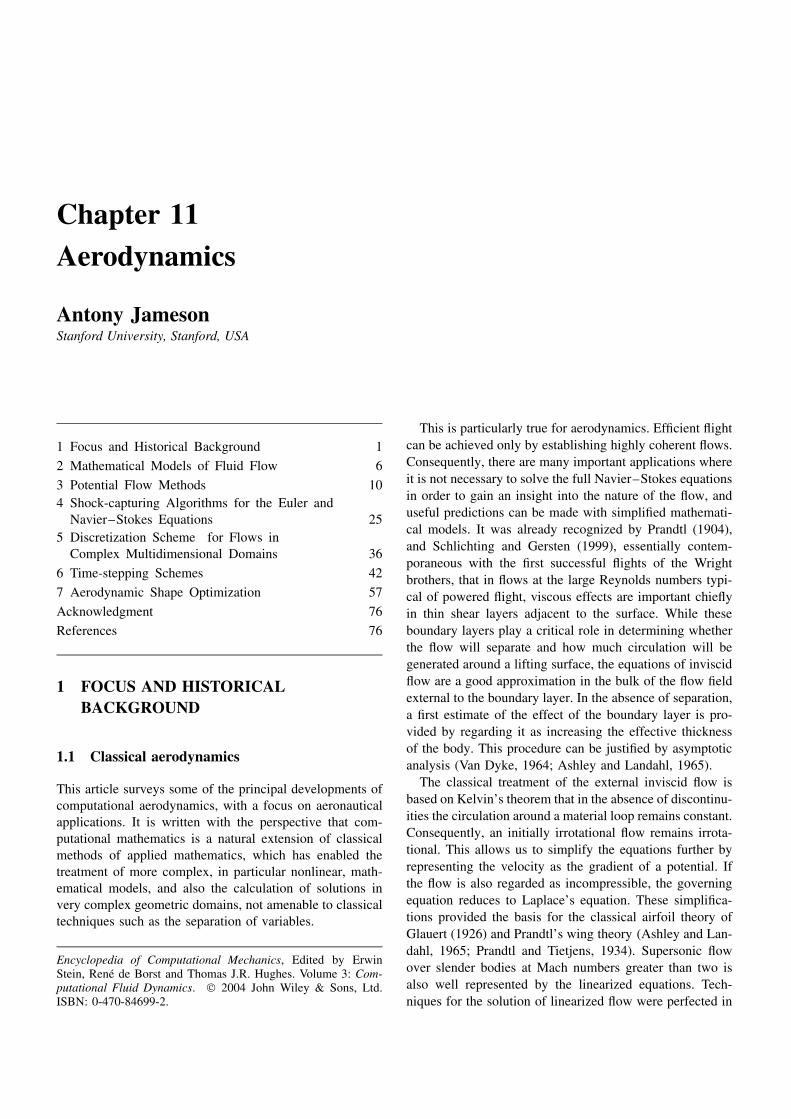
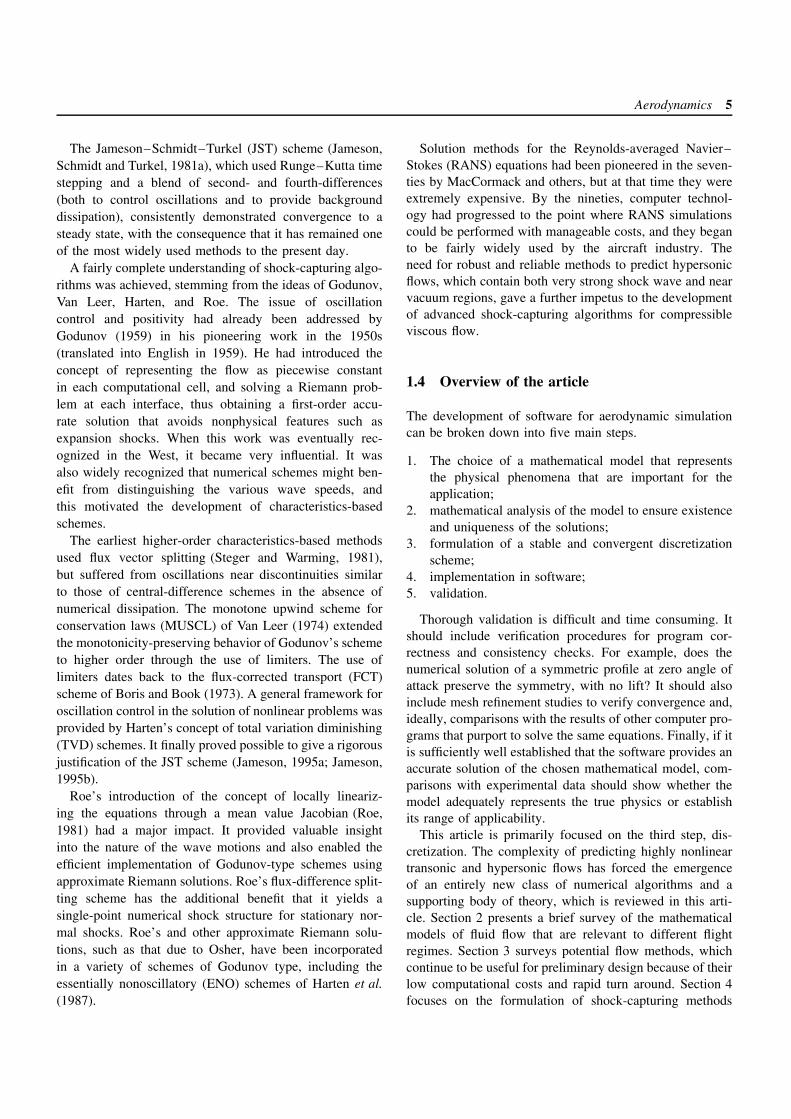
Here V is the speed, L/D is the lift to drag ratio, sfc isthe specific fuel consumption of the engines, W0 is thelanding weight, and Wf is the weight of the fuel burnt.The Breguet equation clearly exposes the multidisciplinarynature of the design problem. A lightweight structure isneeded to minimize W0. The specific fuel consumption ismainly the province of the engine manufacturers, and infact, the largest advances during the last 30 years have beenin engine efficiency. The aerodynamic designer should tryto maximize VL/D. This means that the cruising speedshould be increased until the onset of drag rise due to theformation of shock waves. Consequently, the best cruis-ing speed is the transonic regime. The typical patternof transonic flow over a wing section is illustrated inFigure 1.
Transonic flow had proved essentially intractable to ana-lytic methods. Garabedian and Korn had demonstratedthe feasibility of designing airfoils for shock-free flow inthe transonic regime numerically by the method of com-plex characteristics (Bauer, Garabedian and Korn, 1972).Their method was formulated in the hodograph plane,and it required great skill to obtain solutions correspond-ing to physically realizable shapes. It was also knownfrom Morawetz’s theorem (Morawetz, 1956) that shock-free transonic solutions are isolated points.
A major breakthrough was accomplished by Murman andCole (1971) with their development of type-dependent dif-ferencing in 1970. They obtained stable solutions by simplyswitching from central differencing in the subsonic zoneto upwind differencing in the supersonic zone and using
Sonic line
Shock wave
Boundary layer
M < 1 M > 1
Figure 1. Transonic flow past an airfoil.
Aerodynamics 3
−4
−2
−1 0
Ks = 1.3
1
0
2
Cp
Cp*
X
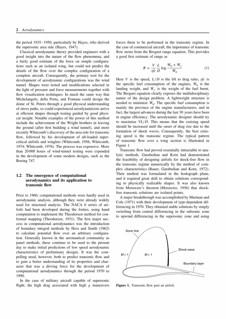
Figure 2. Scaled pressure coefficient on surface of a thin,circular-arc airfoil in transonic flow, compared with experimentaldata; solid line represents computational result.
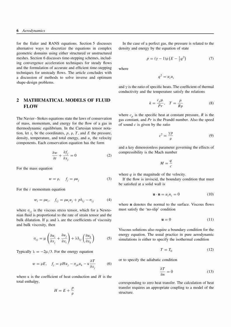
a line-implicit relaxation scheme. Their discovery providedmajor impetus for the further development of computationalfluid dynamics (CFD) by demonstrating that solutions forsteady transonic flows could be computed economically.Figure 2 taken from their landmark paper illustrates thescaled pressure distribution on the surface of a symmetricairfoil. Efforts were soon underway to extend their ideas tomore general transonic flows.
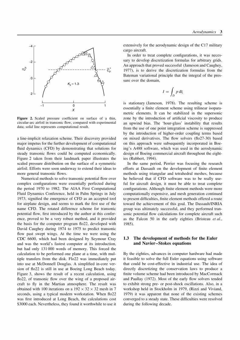
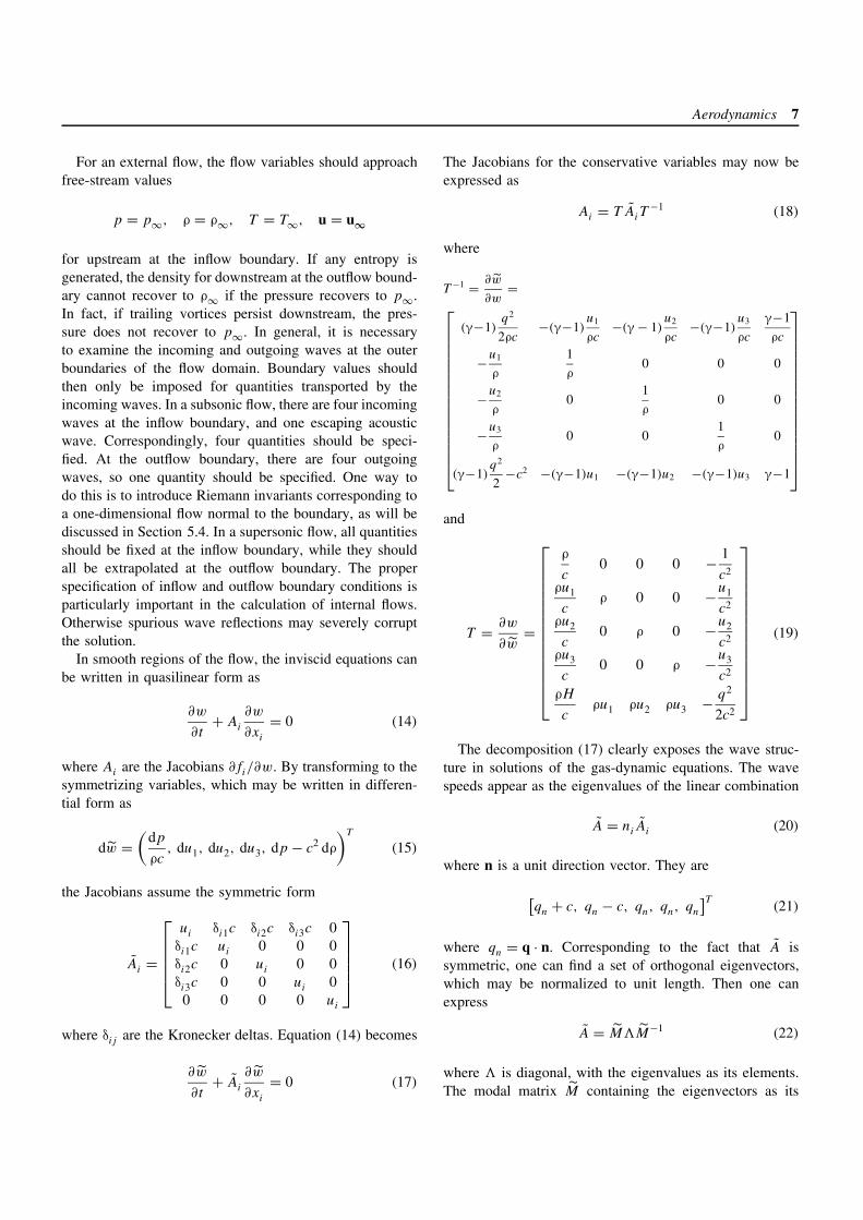
Numerical methods to solve transonic potential flow overcomplex configurations were essentially perfected duringthe period 1970 to 1982. The AIAA First ComputationalFluid Dynamics Conference, held in Palm Springs in July1973, signified the emergence of CFD as an accepted toolfor airplane design, and seems to mark the first use of thename CFD. The rotated difference scheme for transonicpotential flow, first introduced by the author at this confer-ence, proved to be a very robust method, and it providedthe basis for the computer program flo22, developed withDavid Caughey during 1974 to 1975 to predict transonicflow past swept wings. At the time we were using theCDC 6600, which had been designed by Seymour Crayand was the world’s fastest computer at its introduction,but had only 131 000 words of memory. This forced thecalculation to be performed one plane at a time, with mul-tiple transfers from the disk. Flo22 was immediately putinto use at McDonnell Douglas. A simplified in-core ver-sion of flo22 is still in use at Boeing Long Beach today.Figure 3, shows the result of a recent calculation, usingflo22, of transonic flow over the wing of a proposed air-craft to fly in the Martian atmosphere. The result wasobtained with 100 iterations on a 192 × 32 × 32 mesh in 7seconds, using a typical modern workstation. When flo22was first introduced at Long Beach, the calculations cost$3000 each. Nevertheless, they found it worthwhile to use it
extensively for the aerodynamic design of the C17 militarycargo aircraft.
In order to treat complete configurations, it was neces-sary to develop discretization formulas for arbitrary grids.An approach that proved successful (Jameson and Caughey,1977), is to derive the discretization formulas from theBateman variational principle that the integral of the pres-sure over the domain,
I =∫
D
p dξ
is stationary (Jameson, 1978). The resulting scheme isessentially a finite element scheme using trilinear isopara-metric elements. It can be stabilized in the supersoniczone by the introduction of artificial viscosity to producean upwind bias. The ‘hour-glass’ instability that resultsfrom the use of one point integration scheme is suppressedby the introduction of higher-order coupling terms basedon mixed derivatives. The flow solvers (flo27-30) basedon this approach were subsequently incorporated in Boe-ing’s A488 software, which was used in the aerodynamicdesign of Boeing commercial aircraft throughout the eight-ies (Rubbert, 1994).
In the same period, Perrier was focusing the researchefforts at Dassault on the development of finite elementmethods using triangular and tetrahedral meshes, becausehe believed that if CFD software was to be really use-ful for aircraft design, it must be able to treat completeconfigurations. Although finite element methods were morecomputationally expensive, and mesh generation continuedto present difficulties, finite element methods offered a routetoward the achievement of this goal. The Dassault/INRIAgroup was ultimately successful, and they performed tran-sonic potential flow calculations for complete aircraft suchas the Falcon 50 in the early eighties (Bristeau et al.,1985).
1.3 The development of methods for the Eulerand Navier–Stokes equations
By the eighties, advances in computer hardware had madeit feasible to solve the full Euler equations using softwarethat could be cost-effective in industrial use. The idea ofdirectly discretizing the conservation laws to produce afinite volume scheme had been introduced by MacCormackand Paullay (1972). Most of the early flow solvers tendedto exhibit strong pre- or post-shock oscillations. Also, in aworkshop held in Stockholm in 1979, (Rizzi and Viviand,1979) it was apparent that none of the existing schemesconverged to a steady state. These difficulties were resolvedduring the following decade.
4 Aerodynamics
Sym
bol
Sou
rce
FLO
−22
+ L/
NM
+ S
Alp
ha
6.7
00
C
D
.031
9
C
M
−0.0
1225
Com
paris
on o
f cho
rdw
ise
pres
sure
dis
trib
utio
nsba
selin
e M
AR
S00
flyi
ng w
ing
conf
igur
atio
nM
ach
= 0.
650,
CL
= 0.
615
Sol
utio
n 1
uppe
r-su
rfac
e is
obar
s(c
onto
urs
at 0
.05
Cp)
0.2
0.4
0.6
0.8
1.0
−2.0
−1.5
−1.0
−0.5 0.0
0.5
1.0
0.0
0.5
1.0
Cp −2.0
−1.5
−1.0
−0.5 0.0
0.5
1.0
Cp
−2.0
−1.5
−1.0
−0.5
Cp
X /
C
X /
C
X /
C14
.6%
spa
n
39.0
% s
pan
0.2
0.4
0.6
0.8
1.0
−2.0
−1.5
−1.0
−0.5 0.0
0.5
1.0
Cp
X /
C
X /
C
X /
C 92.
7% s
pan
0.2
0.4
0.6
0.8
1.0
−2.0
−1.5
−1.0
−0.5 0.0
0.5
1.0
Cp
78.
0% s
pan
0.2
0.4
0.6
0.8
1.0
24.4
% s
pan
0.2
0.4
0.6
0.8
1.0
−2.0
−1.5
−1.0
−0.5 0.0
0.5
1.0
Cp
X /
C0.
20.
40.
60.
81.
0
0.0%
spa
n
0.2
0.4
0.6
0.8
1.0
−2.0
−1.5
−1.0
−0.5 0.0
0.5
1.0
Cp
63.4
spa
n
0.2
0.4
0.6
0.8
1.0
−2.0
−1.5
−1.0
−0.5 0.0
0.5
1.0
Cp
X /
C53
.7%
spa
n
Fig
ure
3.Pr
essu
redi
stri
butio
nov
erth
ew
ing
ofa
Mar
sL
ande
rus
ing
flo22
(sup
plie
dby
John
Vas
sber
g).
Aerodynamics 5
The Jameson–Schmidt–Turkel (JST) scheme (Jameson,Schmidt and Turkel, 1981a), which used Runge–Kutta timestepping and a blend of second- and fourth-differences(both to control oscillations and to provide backgrounddissipation), consistently demonstrated convergence to asteady state, with the consequence that it has remained oneof the most widely used methods to the present day.
A fairly complete understanding of shock-capturing algo-rithms was achieved, stemming from the ideas of Godunov,Van Leer, Harten, and Roe. The issue of oscillationcontrol and positivity had already been addressed byGodunov (1959) in his pioneering work in the 1950s(translated into English in 1959). He had introduced theconcept of representing the flow as piecewise constantin each computational cell, and solving a Riemann prob-lem at each interface, thus obtaining a first-order accu-rate solution that avoids nonphysical features such asexpansion shocks. When this work was eventually rec-ognized in the West, it became very influential. It wasalso widely recognized that numerical schemes might ben-efit from distinguishing the various wave speeds, andthis motivated the development of characteristics-basedschemes.
The earliest higher-order characteristics-based methodsused flux vector splitting (Steger and Warming, 1981),but suffered from oscillations near discontinuities similarto those of central-difference schemes in the absence ofnumerical dissipation. The monotone upwind scheme forconservation laws (MUSCL) of Van Leer (1974) extendedthe monotonicity-preserving behavior of Godunov’s schemeto higher order through the use of limiters. The use oflimiters dates back to the flux-corrected transport (FCT)scheme of Boris and Book (1973). A general framework foroscillation control in the solution of nonlinear problems wasprovided by Harten’s concept of total variation diminishing(TVD) schemes. It finally proved possible to give a rigorousjustification of the JST scheme (Jameson, 1995a; Jameson,1995b).
Roe’s introduction of the concept of locally lineariz-ing the equations through a mean value Jacobian (Roe,1981) had a major impact. It provided valuable insightinto the nature of the wave motions and also enabled theefficient implementation of Godunov-type schemes usingapproximate Riemann solutions. Roe’s flux-difference split-ting scheme has the additional benefit that it yields asingle-point numerical shock structure for stationary nor-mal shocks. Roe’s and other approximate Riemann solu-tions, such as that due to Osher, have been incorporatedin a variety of schemes of Godunov type, including theessentially nonoscillatory (ENO) schemes of Harten et al.(1987).
Solution methods for the Reynolds-averaged Navier–Stokes (RANS) equations had been pioneered in the seven-ties by MacCormack and others, but at that time they wereextremely expensive. By the nineties, computer technol-ogy had progressed to the point where RANS simulationscould be performed with manageable costs, and they beganto be fairly widely used by the aircraft industry. Theneed for robust and reliable methods to predict hypersonicflows, which contain both very strong shock wave and nearvacuum regions, gave a further impetus to the developmentof advanced shock-capturing algorithms for compressibleviscous flow.
1.4 Overview of the article
The development of software for aerodynamic simulationcan be broken down into five main steps.
1. The choice of a mathematical model that representsthe physical phenomena that are important for theapplication;
2. mathematical analysis of the model to ensure existenceand uniqueness of the solutions;
3. formulation of a stable and convergent discretizationscheme;
4. implementation in software;5. validation.
Thorough validation is difficult and time consuming. Itshould include verification procedures for program cor-rectness and consistency checks. For example, does thenumerical solution of a symmetric profile at zero angle ofattack preserve the symmetry, with no lift? It should alsoinclude mesh refinement studies to verify convergence and,ideally, comparisons with the results of other computer pro-grams that purport to solve the same equations. Finally, if itis sufficiently well established that the software provides anaccurate solution of the chosen mathematical model, com-parisons with experimental data should show whether themodel adequately represents the true physics or establishits range of applicability.
This article is primarily focused on the third step, dis-cretization. The complexity of predicting highly nonlineartransonic and hypersonic flows has forced the emergenceof an entirely new class of numerical algorithms and asupporting body of theory, which is reviewed in this arti-cle. Section 2 presents a brief survey of the mathematicalmodels of fluid flow that are relevant to different flightregimes. Section 3 surveys potential flow methods, whichcontinue to be useful for preliminary design because of theirlow computational costs and rapid turn around. Section 4focuses on the formulation of shock-capturing methods
6 Aerodynamics
for the Euler and RANS equations. Section 5 discussesalternative ways to discretize the equations in complexgeometric domains using either structured or unstructuredmeshes. Section 6 discusses time-stepping schemes, includ-ing convergence acceleration techniques for steady flowsand the formulation of accurate and efficient time-steppingtechniques for unsteady flows. The article concludes witha discussion of methods to solve inverse and optimumshape-design problems.
2 MATHEMATICAL MODELS OF FLUIDFLOW
The Navier–Stokes equations state the laws of conservationof mass, momentum, and energy for the flow of a gas inthermodynamic equilibrium. In the Cartesian tensor nota-tion, let xi be the coordinates, p, ρ, T , and E the pressure,density, temperature, and total energy, and ui the velocitycomponents. Each conservation equation has the form
∂w
∂t+ ∂fj
∂xj
= 0 (2)
For the mass equation
w = ρ, fj = ρuj (3)
For the i momentum equation
wi = ρui, fij = ρuiuj + pδij − σij (4)
where σij is the viscous stress tensor, which for a Newto-nian fluid is proportional to the rate of strain tensor and thebulk dilatation. If µ and λ are the coefficients of viscosityand bulk viscosity, then
σij = µ
(∂ui
∂xj
+ ∂uj
∂xi
)+ λδij
(∂uk
∂xk
)(5)
Typically λ = −2µ/3. For the energy equation
w = ρE, fj = ρHuj − σjkuk − κ∂T
∂xj
(6)
where κ is the coefficient of heat conduction and H is thetotal enthalpy,
H = E + p
ρ
In the case of a perfect gas, the pressure is related to thedensity and energy by the equation of state
p = (γ − 1)ρ(E − 1
2q2) (7)
where
q2 = uiui
and γ is the ratio of specific heats. The coefficient of thermalconductivity and the temperature satisfy the relations
k = cpµ
Pr, T = p
Rρ(8)
where cp is the specific heat at constant pressure, R is thegas constant, and Pr is the Prandtl number. Also the speedof sound c is given by the ratio
c2 = γp
ρ(9)
and a key dimensionless parameter governing the effects ofcompressibility is the Mach number
M = q
c
where q is the magnitude of the velocity.If the flow is inviscid, the boundary condition that must
be satisfied at a solid wall is
u · n = uini = 0 (10)
where n denotes the normal to the surface. Viscous flowsmust satisfy the ‘no-slip’ condition
u = 0 (11)
Viscous solutions also require a boundary condition for theenergy equation. The usual practice in pure aerodynamicsimulations is either to specify the isothermal condition
T = T0 (12)
or to specify the adiabatic condition
∂T
∂n= 0 (13)
corresponding to zero heat transfer. The calculation of heattransfer requires an appropriate coupling to a model of thestructure.
Aerodynamics 7
For an external flow, the flow variables should approachfree-stream values
p = p∞, ρ = ρ∞, T = T∞, u = u∞
for upstream at the inflow boundary. If any entropy isgenerated, the density for downstream at the outflow bound-ary cannot recover to ρ∞ if the pressure recovers to p∞.In fact, if trailing vortices persist downstream, the pres-sure does not recover to p∞. In general, it is necessaryto examine the incoming and outgoing waves at the outerboundaries of the flow domain. Boundary values shouldthen only be imposed for quantities transported by theincoming waves. In a subsonic flow, there are four incomingwaves at the inflow boundary, and one escaping acousticwave. Correspondingly, four quantities should be speci-fied. At the outflow boundary, there are four outgoingwaves, so one quantity should be specified. One way todo this is to introduce Riemann invariants corresponding toa one-dimensional flow normal to the boundary, as will bediscussed in Section 5.4. In a supersonic flow, all quantitiesshould be fixed at the inflow boundary, while they shouldall be extrapolated at the outflow boundary. The properspecification of inflow and outflow boundary conditions isparticularly important in the calculation of internal flows.Otherwise spurious wave reflections may severely corruptthe solution.
In smooth regions of the flow, the inviscid equations canbe written in quasilinear form as
∂w
∂t+ Ai
∂w
∂xi
= 0 (14)
where Ai are the Jacobians ∂fi/∂w. By transforming to thesymmetrizing variables, which may be written in differen-tial form as
dw =(
dp
ρc, du1, du2, du3, dp − c2 dρ
)T
(15)
the Jacobians assume the symmetric form
Ai =
ui δi1c δi2c δi3c 0
δi1c ui 0 0 0δi2c 0 ui 0 0δi3c 0 0 ui 0
0 0 0 0 ui
(16)
where δij are the Kronecker deltas. Equation (14) becomes
∂w
∂t+ Ai
∂w
∂xi
= 0 (17)
The Jacobians for the conservative variables may now beexpressed as
Ai = T AiT−1 (18)
where
T −1 = ∂w
∂w=
(γ−1)q2
2ρc−(γ−1)
u1
ρc−(γ − 1)
u2
ρc−(γ−1)
u3
ρc
γ−1
ρc
−u1
ρ
1
ρ0 0 0
−u2
ρ0
1
ρ0 0
−u3
ρ0 0
1
ρ0
(γ−1)q2
2−c2 −(γ−1)u1 −(γ−1)u2 −(γ−1)u3 γ−1
and
T = ∂w
∂w=
ρ
c0 0 0 − 1
c2
ρu1
cρ 0 0 −u1
c2
ρu2
c0 ρ 0 −u2
c2
ρu3
c0 0 ρ −u3
c2
ρH
cρu1 ρu2 ρu3 − q2
2c2
(19)
The decomposition (17) clearly exposes the wave struc-ture in solutions of the gas-dynamic equations. The wavespeeds appear as the eigenvalues of the linear combination
A = niAi (20)
where n is a unit direction vector. They are
[qn + c, qn − c, qn, qn, qn
]T(21)
where qn = q · n. Corresponding to the fact that A issymmetric, one can find a set of orthogonal eigenvectors,which may be normalized to unit length. Then one canexpress
A = M�M−1 (22)
where � is diagonal, with the eigenvalues as its elements.The modal matrix M containing the eigenvectors as its
8 Aerodynamics
columns is
M =
1√2
− 1√2
0 0 0
n1√2
n1√2
0 −n3 n2
n2√2
n2√2
n3 0 −n1
n3√2
n3√2
−n2 n1 0
0 0 n1 n2 n3
(23)
and M−1 = MT . The Jacobian matrix A = niAi now takesthe form
A = M�M−1 (24)
where
M = T M, M−1 = MT T −1 (25)
In the design of difference schemes, it proves useful tointroduce the absolute Jacobian matrix |A|, in which theeigenvalues are replaced by their absolute values, as willbe discussed in Section 4.4.
Corresponding to the thermodynamic relation
dp
ρ= dh − T dS
where S is the entropy log(p/ργ−1), the last variable of dw
corresponds to p dS, since c2 = (dp/dρ). It follows that inthe absence of shock waves S is constant along streamlines.If the flow is isentropic, then (dp/dρ) ∝ ργ−1, and the firstvariable can be integrated to give 2c/(γ − 1). Then we maytake the transformed variables as
w =(
2c
γ − 1, u1, u2, u3,S
)T
(26)
In the case of a one-dimensional flow, the equations for theRiemann invariants are recovered by adding and subtractingthe equations for 2c/(γ − 1) and u1.
In order to calculate solutions for flows in complex geo-metric domains, it is often useful to introduce body-fittedcoordinates through global, or, as in the case of isopara-metric elements, local transformations. With the body nowcoinciding with a coordinate surface, it is much easier toenforce the boundary conditions accurately. Suppose thatthe mapping to computational coordinates (ξ1, ξ2, ξ3) isdefined by the transformation matrices
Kij = ∂xi
∂ξj
, K−1ij = ∂ξi
∂xj
, J = det(K) (27)
The Navier–Stokes equations (2–6) become
∂
∂t(Jw) + ∂
∂ξi
Fi(w) = 0 (28)
Here the transformed fluxes are
Fi = Sijfj (29)
where
S = JK−1 (30)
The elements of S are the cofactors of K , and in afinite volume discretization, they are just the face areasof the computational cells projected in the x1, x2, and x3directions. Using the permutation tensor εijk we can expressthe elements of S as
Sij = 1
2εjpqεirs
∂xp
∂ξr
∂xq
∂ξs
(31)
Then
∂
∂ξi
Sij = 1
2εjpqεirs
(∂2xp
∂ξr∂ξi
∂xq
∂ξs
+ ∂xp
∂ξr
∂2xq
∂ξs∂ξi
)= 0 (32)
Defining scaled contravariant velocity components as
Ui = Sijuj (33)
the flux formulas may be expanded as
Fi =
ρUi
ρUiu1 + Si1p
ρUiu2 + Si2p
ρUiu3 + Si3p
ρUiH
(34)
If we choose a coordinate system so that the boundary isat ξl = 0, the wall boundary condition for inviscid flow isnow
Ul = 0 (35)
An indication of the relative magnitude of the inertialand viscous terms is given by the Reynolds number
Re = ρUL
µ(36)
where U is a characteristic velocity and L a representa-tive length. The viscosity of air is very small, and typical
Aerodynamics 9
Reynolds numbers for the flow past a component of anaircraft such as a wing are of the order of 107 or more,depending on the size and speed of the aircraft. In this sit-uation, the viscous effects are essentially confined to thinboundary layers covering the surface. Boundary layers maynevertheless have a global impact on the flow by caus-ing separation. Unfortunately, unless they are controlledby active means such as suction through a porous sur-face, boundary layers are unstable and generally becometurbulent.
Using dimensional analysis, Kolmogorov’s theory of tur-bulence (Kolmogorov, 1941) estimates the length scales ofthe smallest persisting eddies to be of order (1/Re3/4) incomparison with the macroscopic length scale of the flow.Accordingly the computational requirements for the fullsimulation of all scales of turbulence can be estimated asgrowing proportionally to Re9/4, and are clearly beyond thereach of current computers. Turbulent flows may be sim-ulated by the RANS equations, where statistical averagesare taken of rapidly fluctuating components. Denoting fluc-tuating parts by primes and averaging by an overbar, thisleads to the appearance of Reynolds stress terms of theform ρu′
iu′j , which cannot be determined from the mean
values of the velocity and density. Estimates of these addi-tional terms must be provided by a turbulence model. Thesimplest turbulence models augment the molecular viscos-ity by an eddy viscosity that crudely represents the effectsof turbulent mixing, and is estimated with some character-istic length scale such as the boundary layer thickness. Arather more elaborate class of models introduces two addi-tional equations for the turbulent kinetic energy and the rateof dissipation. Existing turbulence models are adequate forparticular classes of flow for which empirical correlationsare available, but they are generally not capable of reli-ably predicting more complex phenomena, such as shockwave–boundary layer interaction. The current status of tur-bulence modeling is reviewed by Wilcox (1998), Haaseet al. (1997), Leschziner (2003), and Durbin in an articlein this Encyclopedia.
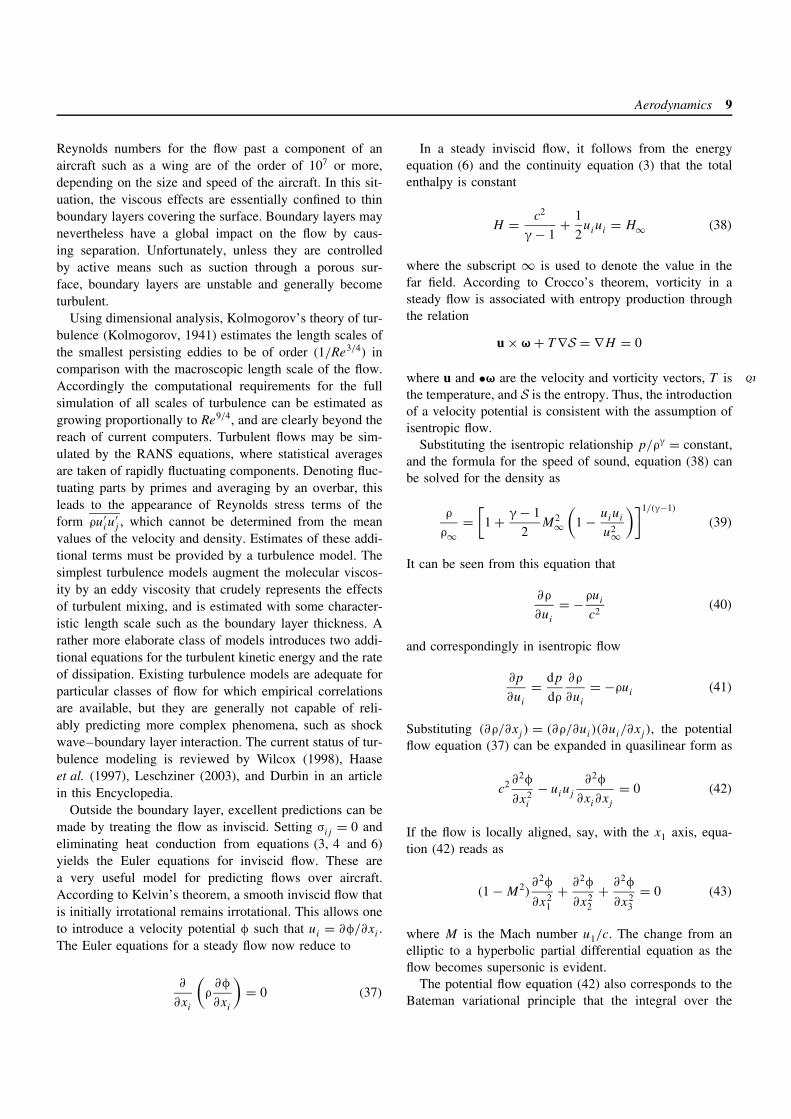
Outside the boundary layer, excellent predictions can bemade by treating the flow as inviscid. Setting σij = 0 andeliminating heat conduction from equations (3, 4 and 6)yields the Euler equations for inviscid flow. These area very useful model for predicting flows over aircraft.According to Kelvin’s theorem, a smooth inviscid flow thatis initially irrotational remains irrotational. This allows oneto introduce a velocity potential φ such that ui = ∂φ/∂xi .The Euler equations for a steady flow now reduce to
∂
∂xi
(ρ
∂φ
∂xi
)= 0 (37)
In a steady inviscid flow, it follows from the energyequation (6) and the continuity equation (3) that the totalenthalpy is constant
H = c2
γ − 1+ 1
2uiui = H∞ (38)
where the subscript ∞ is used to denote the value in thefar field. According to Crocco’s theorem, vorticity in asteady flow is associated with entropy production throughthe relation
u × ω + T ∇S = ∇H = 0
where u and •ω are the velocity and vorticity vectors, T is Q1
the temperature, and S is the entropy. Thus, the introductionof a velocity potential is consistent with the assumption ofisentropic flow.
Substituting the isentropic relationship p/ργ = constant,and the formula for the speed of sound, equation (38) canbe solved for the density as
ρ
ρ∞=
[1 + γ − 1
2M2
∞
(1 − uiui
u2∞
)]1/(γ−1)
(39)
It can be seen from this equation that
∂ρ
∂ui
= −ρui
c2(40)
and correspondingly in isentropic flow
∂p
∂ui
= dp
dρ
∂ρ
∂ui
= −ρui (41)
Substituting (∂ρ/∂xj ) = (∂ρ/∂ui)(∂ui/∂xj ), the potentialflow equation (37) can be expanded in quasilinear form as
c2 ∂2φ
∂x2i
− uiuj
∂2φ
∂xi∂xj
= 0 (42)
If the flow is locally aligned, say, with the x1 axis, equa-tion (42) reads as
(1 − M2)∂2φ
∂x21
+ ∂2φ
∂x22
+ ∂2φ
∂x23
= 0 (43)
where M is the Mach number u1/c. The change from anelliptic to a hyperbolic partial differential equation as theflow becomes supersonic is evident.
The potential flow equation (42) also corresponds to theBateman variational principle that the integral over the
10 Aerodynamics
domain of the pressure
I =∫
D
p dξ (44)
is stationary. Here dξ denotes the volume element. Usingthe relation (41), a variation δp results in a variation
δI =∫
D
∂p
∂ui
δui dξ = −∫
ρui
∂
∂xi
δφ dξ
or, on integrating by parts with appropriate boundary con-ditions
δI =∫
D
∂
∂xi
(ρ
∂φ
∂xi
)δφ dξ
Then δI = 0 for an arbitrary variation δφ if equation (37)holds.
The equations of inviscid supersonic flow admit discon-tinuous solutions, both shock waves and contact discon-tinuities, which satisfy the Rankine Hugoniot jump con-ditions (Liepmann and Roshko, 1957). Only compressionshock waves are admissible, corresponding to the pro-duction of entropy. Expansion shock waves cannot occurbecause they would correspond to a decrease in entropy.
Because shock waves generate entropy, they cannotbe exactly modeled by the potential flow equations. Theamount of entropy generated is proportional to (M − 1)3
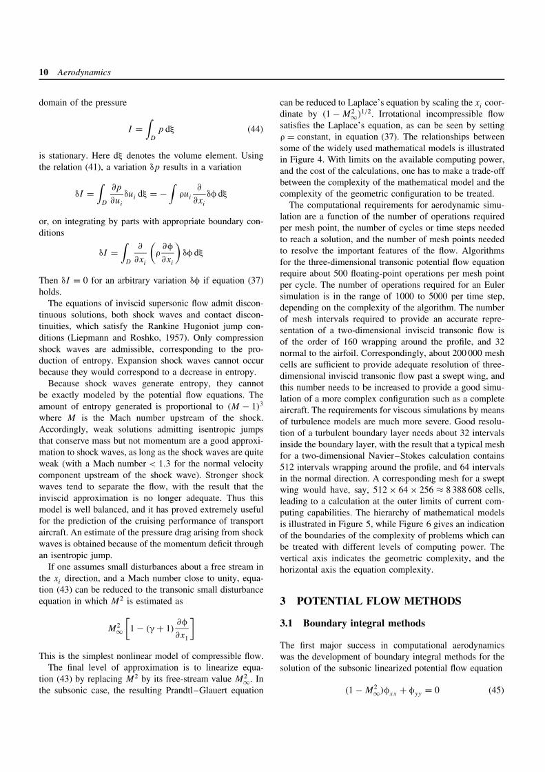
where M is the Mach number upstream of the shock.Accordingly, weak solutions admitting isentropic jumpsthat conserve mass but not momentum are a good approxi-mation to shock waves, as long as the shock waves are quiteweak (with a Mach number < 1.3 for the normal velocitycomponent upstream of the shock wave). Stronger shockwaves tend to separate the flow, with the result that theinviscid approximation is no longer adequate. Thus thismodel is well balanced, and it has proved extremely usefulfor the prediction of the cruising performance of transportaircraft. An estimate of the pressure drag arising from shockwaves is obtained because of the momentum deficit throughan isentropic jump.
If one assumes small disturbances about a free stream inthe xi direction, and a Mach number close to unity, equa-tion (43) can be reduced to the transonic small disturbanceequation in which M2 is estimated as
M2∞
[1 − (γ + 1)
∂φ
∂x1
]This is the simplest nonlinear model of compressible flow.
The final level of approximation is to linearize equa-tion (43) by replacing M2 by its free-stream value M2∞. Inthe subsonic case, the resulting Prandtl–Glauert equation
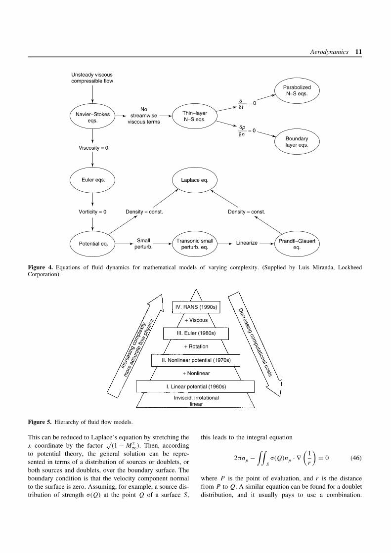
can be reduced to Laplace’s equation by scaling the xi coor-dinate by (1 − M2∞)1/2. Irrotational incompressible flowsatisfies the Laplace’s equation, as can be seen by settingρ = constant, in equation (37). The relationships betweensome of the widely used mathematical models is illustratedin Figure 4. With limits on the available computing power,and the cost of the calculations, one has to make a trade-offbetween the complexity of the mathematical model and thecomplexity of the geometric configuration to be treated.
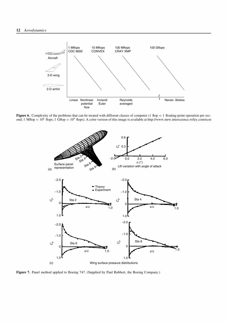
The computational requirements for aerodynamic simu-lation are a function of the number of operations requiredper mesh point, the number of cycles or time steps neededto reach a solution, and the number of mesh points neededto resolve the important features of the flow. Algorithmsfor the three-dimensional transonic potential flow equationrequire about 500 floating-point operations per mesh pointper cycle. The number of operations required for an Eulersimulation is in the range of 1000 to 5000 per time step,depending on the complexity of the algorithm. The numberof mesh intervals required to provide an accurate repre-sentation of a two-dimensional inviscid transonic flow isof the order of 160 wrapping around the profile, and 32normal to the airfoil. Correspondingly, about 200 000 meshcells are sufficient to provide adequate resolution of three-dimensional inviscid transonic flow past a swept wing, andthis number needs to be increased to provide a good simu-lation of a more complex configuration such as a completeaircraft. The requirements for viscous simulations by meansof turbulence models are much more severe. Good resolu-tion of a turbulent boundary layer needs about 32 intervalsinside the boundary layer, with the result that a typical meshfor a two-dimensional Navier–Stokes calculation contains512 intervals wrapping around the profile, and 64 intervalsin the normal direction. A corresponding mesh for a sweptwing would have, say, 512 × 64 × 256 ≈ 8 388 608 cells,leading to a calculation at the outer limits of current com-puting capabilities. The hierarchy of mathematical modelsis illustrated in Figure 5, while Figure 6 gives an indicationof the boundaries of the complexity of problems which canbe treated with different levels of computing power. Thevertical axis indicates the geometric complexity, and thehorizontal axis the equation complexity.
3 POTENTIAL FLOW METHODS
3.1 Boundary integral methods
The first major success in computational aerodynamicswas the development of boundary integral methods for thesolution of the subsonic linearized potential flow equation
(1 − M2∞)φxx + φyy = 0 (45)
Aerodynamics 11
pn
δ___
t= 0
= 0δδ___
Viscosity = 0
Linearize
δNo
streamwiseviscous terms
Vorticity = 0 Density = const. Density = const.
Boundarylayer eqs.
Thin−layerN−S eqs.
Navier−Stokeseqs.
Unsteady viscouscompressible flow
Euler eqs. Laplace eq.
ParabolizedN−S eqs.
Prandtl−Glauerteq.
Potential eq.Small
perturb.Transonic small
perturb. eq.
Figure 4. Equations of fluid dynamics for mathematical models of varying complexity. (Supplied by Luis Miranda, LockheedCorporation).
IV. RANS (1990s)
Incr
easi
ng c
ompl
exity
mor
e ac
cura
te fl
ow p
hysi
cs
III. Euler (1980s)
Decreasing com
putational costs
II. Nonlinear potential (1970s)
I. Linear potential (1960s)
Inviscid, irrotationallinear
+ Viscous
+ Rotation
+ Nonlinear
Figure 5. Hierarchy of fluid flow models.
This can be reduced to Laplace’s equation by stretching thex coordinate by the factor
√(1 − M2∞). Then, according
to potential theory, the general solution can be repre-sented in terms of a distribution of sources or doublets, orboth sources and doublets, over the boundary surface. Theboundary condition is that the velocity component normalto the surface is zero. Assuming, for example, a source dis-tribution of strength σ(Q) at the point Q of a surface S,
this leads to the integral equation
2πσp −∫∫
S
σ(Q)np · ∇(
1
r
)= 0 (46)
where P is the point of evaluation, and r is the distancefrom P to Q. A similar equation can be found for a doubletdistribution, and it usually pays to use a combination.
12 Aerodynamics
Linear
1 MflopsCDC 6600
100 Gflops100 MflopsCRAY XMP
10 MflopsCONVEX
InviscidEuler
Nonlinearpotential
flow
Navier−StokesReynoldsaveraged
2-D airfoil
3-D wing
Aircraft
Figure 6. Complexity of the problems that can be treated with different classes of computer (1 flop = 1 floating-point operation per sec-ond; 1 Mflop = 106 flops; 1 Gflop = 109 flops). A color version of this image is available at http://www.mrw.interscience.wiley.com/ecm
Wing surface pressure distributions
ExperimentTheory
−2.0
−1.0
1.0
0Sta 2C
p
x /c
−2.0
−1.0
1.0
1.0
0x/c
Sta 6Cp
−2.0
−1.0
1.0
0
Cp
1.0
Sta 4
−1.0
1.0
0
−2.0
Cp
1.0
Sta 8
(c)
0.3
−2.0 0.0 2.0α (°)
Lift variation with angle of attack
4.0 6.0
CL
0.6
(b)
1.0 x/c
x/c
Surface panelrepresentation
Sta 2
Sta 4
Sta 6
Sta 8(a)
Figure 7. Panel method applied to Boeing 747. (Supplied by Paul Rubbert, the Boeing Company.)
Aerodynamics 13
Equation (46) can be reduced to a set of algebraic equationsby dividing the surface into quadrilateral panels, assuminga constant source strength on each panel, and satisfyingthe condition of zero normal velocity at the center of eachpanel. This leads to N equations for the source strengths onN panels.
The first such method was introduced by Hess and Smith(1962). The method was extended to lifting flows, togetherwith the inclusion of doublet distributions, by Rubbert andSaaris (1968). Subsequently higher-order panel methods (asthese methods are generally called in the aircraft industry)have been introduced. A review has been given by Hunt(1978). An example of a calculation by a panel method isshown in Figure 7. The results are displayed in terms ofthe pressure coefficient defined as
cp = p − p∞12ρ∞q2∞
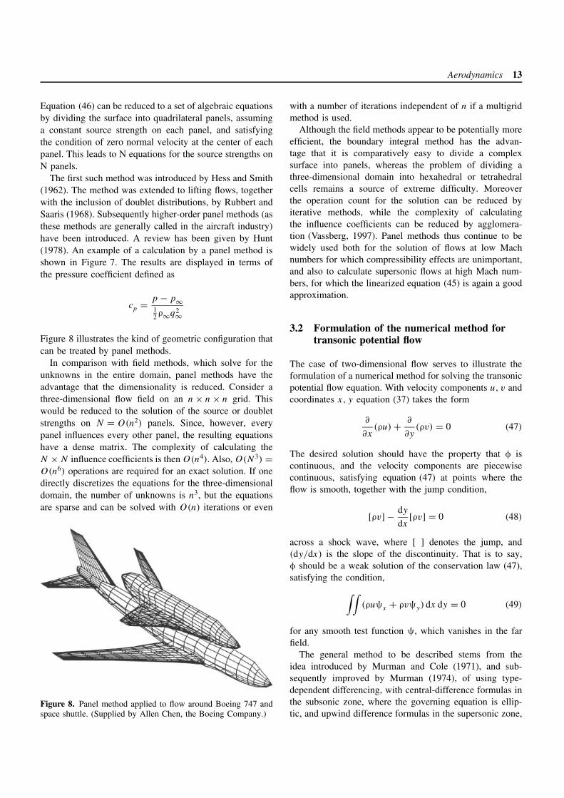
Figure 8 illustrates the kind of geometric configuration thatcan be treated by panel methods.
In comparison with field methods, which solve for theunknowns in the entire domain, panel methods have theadvantage that the dimensionality is reduced. Consider athree-dimensional flow field on an n × n × n grid. Thiswould be reduced to the solution of the source or doubletstrengths on N = O(n2) panels. Since, however, everypanel influences every other panel, the resulting equationshave a dense matrix. The complexity of calculating theN × N influence coefficients is then O(n4). Also, O(N3) =O(n6) operations are required for an exact solution. If onedirectly discretizes the equations for the three-dimensionaldomain, the number of unknowns is n3, but the equationsare sparse and can be solved with O(n) iterations or even
Figure 8. Panel method applied to flow around Boeing 747 andspace shuttle. (Supplied by Allen Chen, the Boeing Company.)
with a number of iterations independent of n if a multigridmethod is used.
Although the field methods appear to be potentially moreefficient, the boundary integral method has the advan-tage that it is comparatively easy to divide a complexsurface into panels, whereas the problem of dividing athree-dimensional domain into hexahedral or tetrahedralcells remains a source of extreme difficulty. Moreoverthe operation count for the solution can be reduced byiterative methods, while the complexity of calculatingthe influence coefficients can be reduced by agglomera-tion (Vassberg, 1997). Panel methods thus continue to bewidely used both for the solution of flows at low Machnumbers for which compressibility effects are unimportant,and also to calculate supersonic flows at high Mach num-bers, for which the linearized equation (45) is again a goodapproximation.
3.2 Formulation of the numerical method fortransonic potential flow
The case of two-dimensional flow serves to illustrate theformulation of a numerical method for solving the transonicpotential flow equation. With velocity components u, v andcoordinates x, y equation (37) takes the form
∂
∂x(ρu) + ∂
∂y(ρv) = 0 (47)
The desired solution should have the property that φ iscontinuous, and the velocity components are piecewisecontinuous, satisfying equation (47) at points where theflow is smooth, together with the jump condition,
[ρv] − dy
dx[ρv] = 0 (48)
across a shock wave, where [ ] denotes the jump, and(dy/dx) is the slope of the discontinuity. That is to say,φ should be a weak solution of the conservation law (47),satisfying the condition,∫∫
(ρuψx + ρvψy) dx dy = 0 (49)
for any smooth test function ψ, which vanishes in the farfield.
The general method to be described stems from theidea introduced by Murman and Cole (1971), and sub-sequently improved by Murman (1974), of using type-dependent differencing, with central-difference formulas inthe subsonic zone, where the governing equation is ellip-tic, and upwind difference formulas in the supersonic zone,
14 Aerodynamics
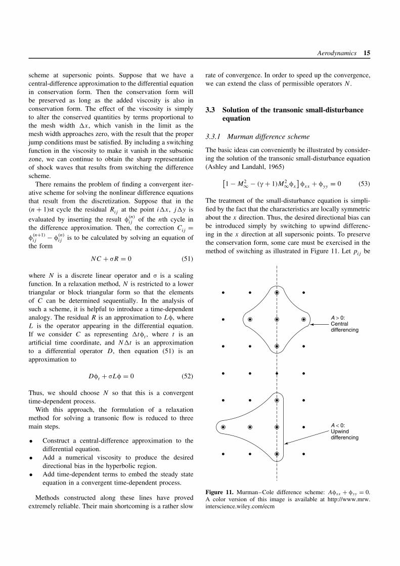
where it is hyperbolic. The resulting directional bias inthe numerical scheme corresponds to the upwind regionof dependence of the flow in the supersonic zone. If weconsider the transonic flow past a profile with fore-and-aft symmetry such as an ellipse, the desired solution ofthe potential flow equation is not symmetric. Instead itexhibits a smooth acceleration over the front half of theprofile, followed by a discontinuous compression througha shock wave. However, the solution of the potential flowequation (42) is invariant under a reversal of the velocityvector, ui = −φxi
. Corresponding to the solution with acompression shock, there is a reverse flow solution with anexpansion shock, as illustrated in Figure 9. In the absenceof a directional bias in the numerical scheme, the fore-and-aft symmetry would be preserved in any solution thatcould be obtained, resulting in the appearance of improperdiscontinuities.
Since the quasilinear form does not distinguish betweenconservation of mass and momentum, difference approxi-mations to it will not necessarily yield solutions that satisfythe jump condition unless shock waves are detected andspecial difference formulas are used in their vicinity. Ifwe treat the conservation law (47), on the other hand, andpreserve the conservation form in the difference approxi-mation, we can ensure that the proper jump condition issatisfied. Similarly, we can obtain proper solutions of thesmall-disturbance equation by treating it in the conservationform.
The general method of constructing a difference approx-imation to a conservation law of the form
fx + gy = 0
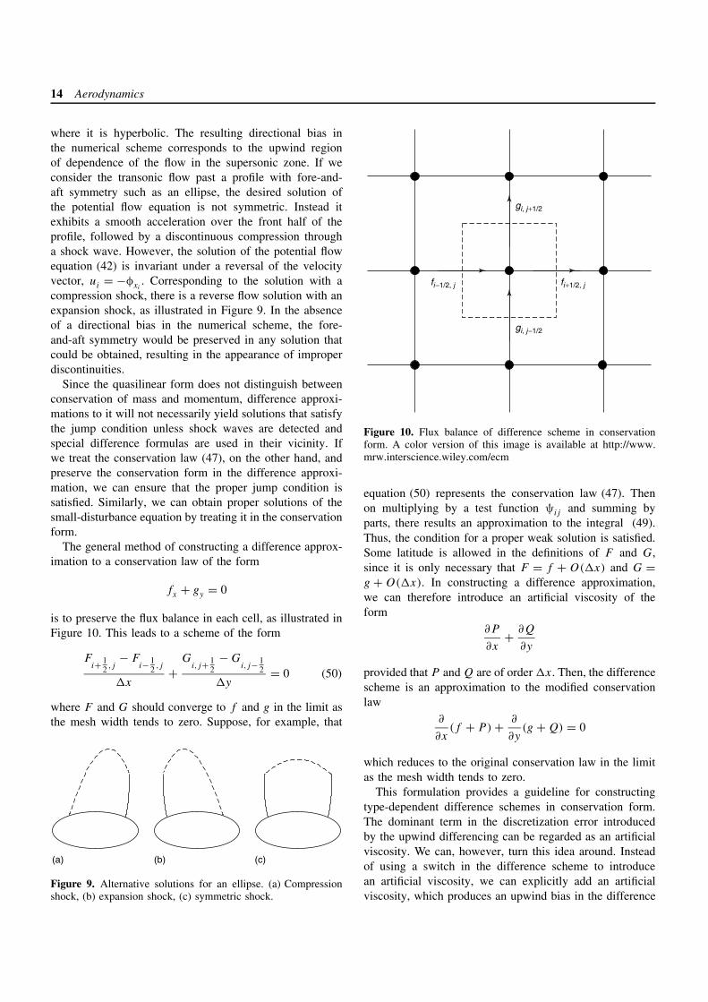
is to preserve the flux balance in each cell, as illustrated inFigure 10. This leads to a scheme of the form
Fi+ 1
2 ,j− F
i− 12 ,j
�x+
Gi,j+ 1
2− G
i,j− 12
�y= 0 (50)
where F and G should converge to f and g in the limit asthe mesh width tends to zero. Suppose, for example, that
(a) (b) (c)
Figure 9. Alternative solutions for an ellipse. (a) Compressionshock, (b) expansion shock, (c) symmetric shock.
gi, j+1/2
gi, j−1/2
fi+1/2, jfi−1/2, j
Figure 10. Flux balance of difference scheme in conservationform. A color version of this image is available at http://www.mrw.interscience.wiley.com/ecm
equation (50) represents the conservation law (47). Thenon multiplying by a test function ψij and summing byparts, there results an approximation to the integral (49).Thus, the condition for a proper weak solution is satisfied.Some latitude is allowed in the definitions of F and G,since it is only necessary that F = f + O(�x) and G =g + O(�x). In constructing a difference approximation,we can therefore introduce an artificial viscosity of theform
∂P
∂x+ ∂Q
∂y
provided that P and Q are of order �x. Then, the differencescheme is an approximation to the modified conservationlaw
∂
∂x(f + P) + ∂
∂y(g + Q) = 0
which reduces to the original conservation law in the limitas the mesh width tends to zero.
This formulation provides a guideline for constructingtype-dependent difference schemes in conservation form.The dominant term in the discretization error introducedby the upwind differencing can be regarded as an artificialviscosity. We can, however, turn this idea around. Insteadof using a switch in the difference scheme to introducean artificial viscosity, we can explicitly add an artificialviscosity, which produces an upwind bias in the difference
Aerodynamics 15
scheme at supersonic points. Suppose that we have acentral-difference approximation to the differential equationin conservation form. Then the conservation form willbe preserved as long as the added viscosity is also inconservation form. The effect of the viscosity is simplyto alter the conserved quantities by terms proportional tothe mesh width �x, which vanish in the limit as themesh width approaches zero, with the result that the properjump conditions must be satisfied. By including a switchingfunction in the viscosity to make it vanish in the subsoniczone, we can continue to obtain the sharp representationof shock waves that results from switching the differencescheme.
There remains the problem of finding a convergent iter-ative scheme for solving the nonlinear difference equationsthat result from the discretization. Suppose that in the(n + 1)st cycle the residual Rij at the point i�x, j�y is
evaluated by inserting the result φ(n)ij of the nth cycle in
the difference approximation. Then, the correction Cij =φ
(n+1)ij − φ
(n)ij is to be calculated by solving an equation of
the form
NC + σR = 0 (51)
where N is a discrete linear operator and σ is a scalingfunction. In a relaxation method, N is restricted to a lowertriangular or block triangular form so that the elementsof C can be determined sequentially. In the analysis ofsuch a scheme, it is helpful to introduce a time-dependentanalogy. The residual R is an approximation to Lφ, whereL is the operator appearing in the differential equation.If we consider C as representing �tφt , where t is anartificial time coordinate, and N�t is an approximationto a differential operator D, then equation (51) is anapproximation to
Dφt + σLφ = 0 (52)
Thus, we should choose N so that this is a convergenttime-dependent process.
With this approach, the formulation of a relaxationmethod for solving a transonic flow is reduced to threemain steps.
• Construct a central-difference approximation to thedifferential equation.
• Add a numerical viscosity to produce the desireddirectional bias in the hyperbolic region.
• Add time-dependent terms to embed the steady stateequation in a convergent time-dependent process.
Methods constructed along these lines have provedextremely reliable. Their main shortcoming is a rather slow
rate of convergence. In order to speed up the convergence,we can extend the class of permissible operators N .
3.3 Solution of the transonic small-disturbanceequation
3.3.1 Murman difference scheme
The basic ideas can conveniently be illustrated by consider-ing the solution of the transonic small-disturbance equation(Ashley and Landahl, 1965)[
1 − M2∞ − (γ + 1)M2
∞φx
]φxx + φyy = 0 (53)
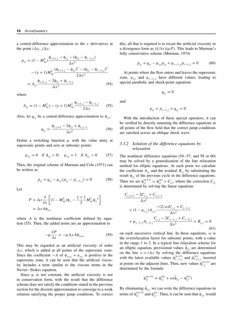
The treatment of the small-disturbance equation is simpli-fied by the fact that the characteristics are locally symmetricabout the x direction. Thus, the desired directional bias canbe introduced simply by switching to upwind differenc-ing in the x direction at all supersonic points. To preservethe conservation form, some care must be exercised in themethod of switching as illustrated in Figure 11. Let pij be
A > 0:Centraldifferencing
A < 0:Upwinddifferencing
Figure 11. Murman–Cole difference scheme: Aφxx + φyy = 0.A color version of this image is available at http://www.mrw.interscience.wiley.com/ecm
16 Aerodynamics
a central-difference approximation to the x derivatives atthe point i�x, j�y:
pij = (1 − M2∞)
φi+1,j − φij − (φij − φi−1,j )
�x2
− (γ + 1)M2∞
(φi+1,j − φij )2 − (φij − φi−1,j )
2
2�x3
= Aij
φi+1,j − 2φij + φi−1,j
�x2(54)
where
Aij = (1 − M2∞) − (γ + 1)M2
∞φi+1,j − φi−1,j
2�x(55)
Also, let qij be a central-difference approximation to φyy :
qij = φi,j+1 − 2φij + φi,j−1
�y2(56)
Define a switching function µ with the value unity atsupersonic points and zero at subsonic points:
µij = 0 if Aij > 0; µij = 1 if Aij < 0 (57)
Then, the original scheme of Murman and Cole (1971) canbe written as
pij + qij − µij (pij − pi−1,j ) = 0 (58)
Let
P = �x∂
∂x
[(1 − M2
∞)φx − γ + 1
2M2
∞φx2]
= �xAφxx
where A is the nonlinear coefficient defined by equa-tion (55). Then, the added terms are an approximation to
−µ∂P
∂x= −µ�xAφxxx (59)
This may be regarded as an artificial viscosity of order�x, which is added at all points of the supersonic zone.Since the coefficient −A of φxxx = uxx is positive in thesupersonic zone, it can be seen that the artificial viscos-ity includes a term similar to the viscous terms in theNavier–Stokes equation.
Since µ is not constant, the artificial viscosity is notin conservation form, with the result that the differencescheme does not satisfy the conditions stated in the previoussection for the discrete approximation to converge to a weaksolution satisfying the proper jump conditions. To correct
this, all that is required is to recast the artificial viscosity ina divergence form as (∂/∂x)(µP). This leads to Murman’sfully conservative scheme (Murman, 1974)
pij + qij − µijpij + µi−1,jpi−1,j = 0 (60)
At points where the flow enters and leaves the supersoniczone, µij and µi−1,j have different values, leading tospecial parabolic and shock-point equations
qij = 0
and
pij + pi−1,j + qij = 0
With the introduction of these special operators, it canbe verified by directly summing the difference equations atall points of the flow field that the correct jump conditionsare satisfied across an oblique shock wave.
3.3.2 Solution of the difference equations byrelaxation
The nonlinear difference equations (54–57, and 58 or 60)may be solved by a generalization of the line relaxationmethod for elliptic equations. At each point we calculatethe coefficient Aij and the residual Rij by substituting theresult φij of the previous cycle in the difference equations.
Then we set φ(n+1)ij = φ
(n)ij + Cij , where the correction Cij
is determined by solving the linear equations
Ci,j+1 − 2Ci,j + Ci,j−1
�y2
+ (1 − µi,j )Ai,j
−(2/ω)Ci,j + Ci−1,j
�x2
+ µi−1,jAi−1,j
Ci,j − 2Ci−1,j + Ci−2,j
�x2+ Ri,j = 0
(61)
on each successive vertical line. In these equations, ω isthe overrelaxation factor for subsonic points, with a valuein the range 1 to 2. In a typical line relaxation scheme foran elliptic equation, provisional values φij are determinedon the line x = i�x by solving the difference equationswith the latest available values φ
(n+1)i−1,j and φ
(n)i+1,j inserted
at points on the adjacent lines. Then, new values φ(n+1)i,j are
determined by the formula
φ(n+1)ij = φ
(n)ij + ω(φij − φ
(n)ij )
By eliminating φij , we can write the difference equations in
terms of φ(n+1)ij and φ
(n)ij . Then, it can be seen that φyy would
Aerodynamics 17
be represented by (1/ω)δ2yφ
(n+1) + [1 − (1/ω)]δ2yφ
(n) insuch a process, where δ2
y denotes the second central-difference operator. The appropriate procedure for treatingthe upwind difference formulas in the supersonic zone,however, is to march in the flow direction, so that the valuesφ
(n+1)ij on each new column can be calculated from the val-
ues φ(n+1)i−2,j and φ
(n+1)i−1,j already determined on the previous
columns. This implies that φyy should be represented byδ2yφ
(n+1) in the supersonic zone, leading to a discontinuityat the sonic line. The correction formula (61) is derived bymodifying this process to remove this discontinuity. Newvalues φ
(n+1)ij are used instead of provisional values φij to
evaluate φyy , at both supersonic and subsonic points. Atsupersonic points, φxx is also evaluated using new values.At subsonic points, φxx is evaluated from φ
(n+1)i−1,j , φ
(n)i+1,j and
a linear combination of φ(n+1)ij and φ
(n)ij . In the subsonic
zone, the scheme acts like a line relaxation scheme, with acomparable rate of convergence. In the supersonic zone, itis equivalent to a marching scheme, once the coefficientsAij have been evaluated. Since the supersonic differencescheme is implicit, no limit is imposed on the step length�x as Aij approaches zero near the sonic line.
3.3.3 Nonunique solutions of the differenceequations for one-dimensional flow
Some of the properties of the Murman difference formulasare clarified by considering a uniform flow in a parallelchannel. Then φyy = 0, and with a suitable normalizationof the potential, the equation reduces to
∂
∂x
(φ2
x
2
)= 0 (62)
with φ and φx given at x = 0, and φ given at x = L.The supersonic zone corresponds to φx > 0. Since φ2
x isconstant, φx simply reverses sign at a jump. Provided weenforce the entropy condition that φx decreases througha jump, there is a unique solution with a single jumpwhenever φx(0) > 0 and φ(0) + Lφx(0) ≥ φ(L) ≥ φ(0) −Lφx(0).
Let ui+1/2 = (φi+1 − φi)/�x and ui = (ui+1/2 +ui−1/2)/2. Then, the fully conservative difference equationscan be written as
Elliptic:
u2
i+ 12
= u2
i− 12
when ui ≤ 0 ui−1 ≤ 0 (a)
Hyperbolic:
u2
i− 12
= u2
i− 32
when ui > 0 ui−1 > 0 (b)
Shock Point:
u2
i+ 12
= u2
i− 32
when ui ≤ 0 ui−1 > 0 (c)
Parabolic:
0 = 0 when ui > 0 ui−1 < 0 (d)
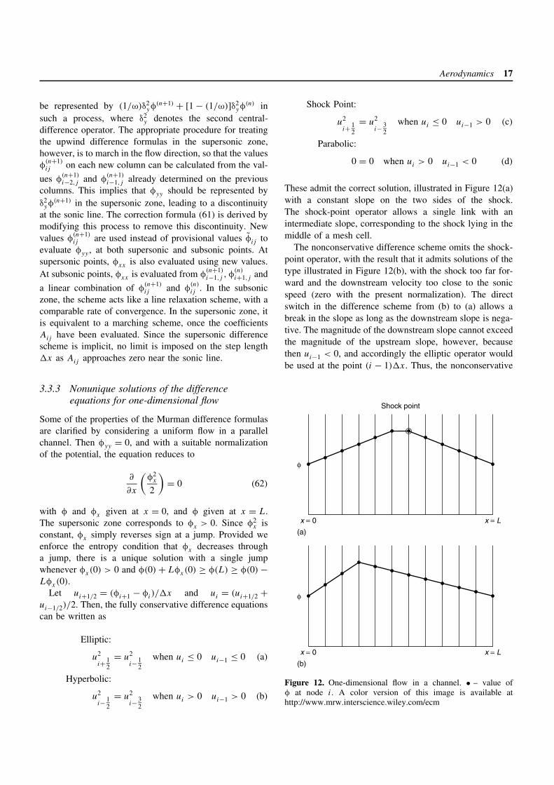
These admit the correct solution, illustrated in Figure 12(a)with a constant slope on the two sides of the shock.The shock-point operator allows a single link with anintermediate slope, corresponding to the shock lying in themiddle of a mesh cell.
The nonconservative difference scheme omits the shock-point operator, with the result that it admits solutions of thetype illustrated in Figure 12(b), with the shock too far for-ward and the downstream velocity too close to the sonicspeed (zero with the present normalization). The directswitch in the difference scheme from (b) to (a) allows abreak in the slope as long as the downstream slope is nega-tive. The magnitude of the downstream slope cannot exceedthe magnitude of the upstream slope, however, becausethen ui−1 < 0, and accordingly the elliptic operator wouldbe used at the point (i − 1)�x. Thus, the nonconservative
(a)
φ
φ
Shock point
x = 0 x = L
(b)
x = 0 x = L
Figure 12. One-dimensional flow in a channel. • – value ofφ at node i. A color version of this image is available athttp://www.mrw.interscience.wiley.com/ecm
18 Aerodynamics
scheme enforces the weakened shock condition,
φi − φi−2 > φi − φi+2 > 0
which allows solutions ranging from the point at which thedownstream velocity is barely subsonic up to the point atwhich the shock strength is correct. When the downstreamvelocity is too close to sonic speed, there is an increasein the mass flow. Thus, the nonconservative scheme mayintroduce a source at the shock wave.
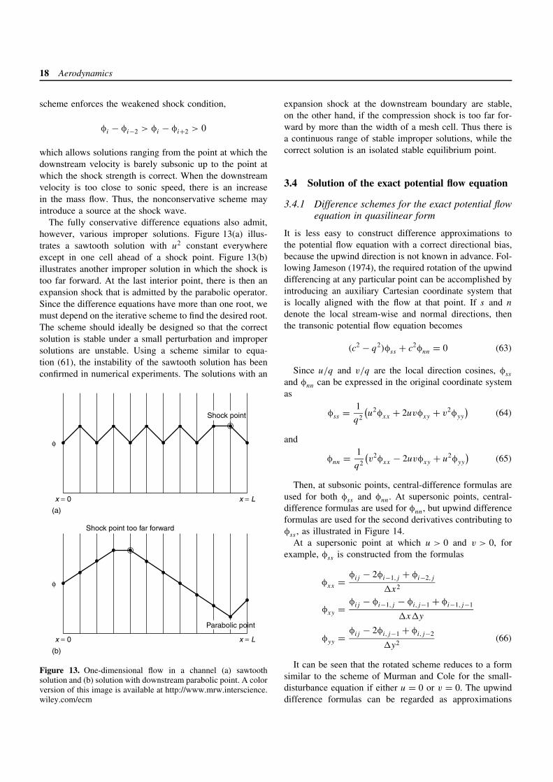
The fully conservative difference equations also admit,however, various improper solutions. Figure 13(a) illus-trates a sawtooth solution with u2 constant everywhereexcept in one cell ahead of a shock point. Figure 13(b)illustrates another improper solution in which the shock istoo far forward. At the last interior point, there is then anexpansion shock that is admitted by the parabolic operator.Since the difference equations have more than one root, wemust depend on the iterative scheme to find the desired root.The scheme should ideally be designed so that the correctsolution is stable under a small perturbation and impropersolutions are unstable. Using a scheme similar to equa-tion (61), the instability of the sawtooth solution has beenconfirmed in numerical experiments. The solutions with an
φ
φ
Shock point too far forward
Parabolic point
Shock point
(a)
x = 0 x = L
(b)
x = 0 x = L
Figure 13. One-dimensional flow in a channel (a) sawtoothsolution and (b) solution with downstream parabolic point. A colorversion of this image is available at http://www.mrw.interscience.wiley.com/ecm
expansion shock at the downstream boundary are stable,on the other hand, if the compression shock is too far for-ward by more than the width of a mesh cell. Thus there isa continuous range of stable improper solutions, while thecorrect solution is an isolated stable equilibrium point.
3.4 Solution of the exact potential flow equation
3.4.1 Difference schemes for the exact potential flowequation in quasilinear form
It is less easy to construct difference approximations tothe potential flow equation with a correct directional bias,because the upwind direction is not known in advance. Fol-lowing Jameson (1974), the required rotation of the upwinddifferencing at any particular point can be accomplished byintroducing an auxiliary Cartesian coordinate system thatis locally aligned with the flow at that point. If s and n
denote the local stream-wise and normal directions, thenthe transonic potential flow equation becomes
(c2 − q2)φss + c2φnn = 0 (63)
Since u/q and v/q are the local direction cosines, φss
and φnn can be expressed in the original coordinate systemas
φss = 1
q2
(u2φxx + 2uvφxy + v2φyy
)(64)
and
φnn = 1
q2
(v2φxx − 2uvφxy + u2φyy
)(65)
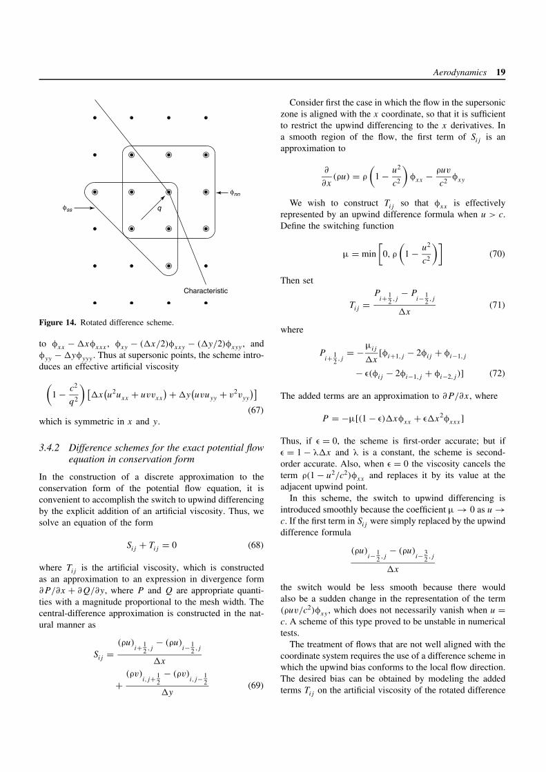
Then, at subsonic points, central-difference formulas areused for both φss and φnn. At supersonic points, central-difference formulas are used for φnn, but upwind differenceformulas are used for the second derivatives contributing toφss , as illustrated in Figure 14.
At a supersonic point at which u > 0 and v > 0, forexample, φss is constructed from the formulas
φxx = φij − 2φi−1,j + φi−2,j
�x2
φxy = φij − φi−1,j − φi,j−1 + φi−1,j−1
�x�y
φyy = φij − 2φi,j−1 + φi,j−2
�y2(66)
It can be seen that the rotated scheme reduces to a formsimilar to the scheme of Murman and Cole for the small-disturbance equation if either u = 0 or v = 0. The upwinddifference formulas can be regarded as approximations
Aerodynamics 19
Characteristic
q
φnn
φss
Figure 14. Rotated difference scheme.
to φxx − �xφxxx , φxy − (�x/2)φxxy − (�y/2)φxyy , andφyy − �yφyyy . Thus at supersonic points, the scheme intro-duces an effective artificial viscosity(
1 − c2
q2
) [�x
(u2uxx + uvvxx
) + �y(uvuyy + v2vyy
)](67)
which is symmetric in x and y.
3.4.2 Difference schemes for the exact potential flowequation in conservation form
In the construction of a discrete approximation to theconservation form of the potential flow equation, it isconvenient to accomplish the switch to upwind differencingby the explicit addition of an artificial viscosity. Thus, wesolve an equation of the form
Sij + Tij = 0 (68)
where Tij is the artificial viscosity, which is constructedas an approximation to an expression in divergence form∂P/∂x + ∂Q/∂y, where P and Q are appropriate quanti-ties with a magnitude proportional to the mesh width. Thecentral-difference approximation is constructed in the nat-ural manner as
Sij =(ρu)
i+ 12 ,j
− (ρu)i− 1
2 ,j
�x
+(ρv)
i,j+ 12
− (ρv)i,j− 1
2
�y(69)
Consider first the case in which the flow in the supersoniczone is aligned with the x coordinate, so that it is sufficientto restrict the upwind differencing to the x derivatives. Ina smooth region of the flow, the first term of Sij is anapproximation to
∂
∂x(ρu) = ρ
(1 − u2
c2
)φxx − ρuv
c2φxy
We wish to construct Tij so that φxx is effectivelyrepresented by an upwind difference formula when u > c.Define the switching function
µ = min[
0, ρ
(1 − u2
c2
)](70)
Then set
Tij =P
i+ 12 ,j
− Pi− 1
2 ,j
�x(71)
where
Pi+ 1
2 ,j= −µij
�x[φi+1,j − 2φij + φi−1,j
− ε(φij − 2φi−1,j + φi−2,j )] (72)
The added terms are an approximation to ∂P/∂x, where
P = −µ[(1 − ε)�xφxx + ε�x2φxxx]
Thus, if ε = 0, the scheme is first-order accurate; but ifε = 1 − λ�x and λ is a constant, the scheme is second-order accurate. Also, when ε = 0 the viscosity cancels theterm ρ(1 − u2/c2)φxx and replaces it by its value at theadjacent upwind point.
In this scheme, the switch to upwind differencing isintroduced smoothly because the coefficient µ → 0 as u →c. If the first term in Sij were simply replaced by the upwinddifference formula
(ρu)i− 1
2 ,j− (ρu)
i− 32 ,j
�x
the switch would be less smooth because there wouldalso be a sudden change in the representation of the term(ρuv/c2)φxy , which does not necessarily vanish when u =c. A scheme of this type proved to be unstable in numericaltests.
The treatment of flows that are not well aligned with thecoordinate system requires the use of a difference scheme inwhich the upwind bias conforms to the local flow direction.The desired bias can be obtained by modeling the addedterms Tij on the artificial viscosity of the rotated difference
20 Aerodynamics
scheme for the quasilinear form described in the previoussection. Since equation (47) is equivalent to equation (63)multiplied by ρ/c2, P and Q should be chosen so that∂P/∂x + ∂Q/∂y contains terms similar to equation (67)multiplied by ρ/c2. The following scheme has provedsuccessful. Let µ be a switching function that vanishes inthe subsonic zone:
µ = max[
0,
(1 − c2
q2
)](73)
Then, P and Q are defined as approximations to
−µ[(1 − ε)u�xρx + εu�x2ρxx
]and
−µ[(1 − ε)v�yρy + εv�y2ρyy]
where the parameter ε controls the accuracy in the sameway as in the simple scheme. If ε = 0, the scheme is first-order accurate, and at a supersonic point where u > 0 andv > 0, P then approximates
−�x
(1 − c2
q2
)uρx = �x
ρ
c2
(1 − c2
q2
)(u2ux + uvvx)
When this formula and the corresponding formula forQ are inserted in ∂P/∂x + ∂Q/∂y, it can be verifiedthat the terms containing the highest derivatives of φ arethe same as those in equation (67) multiplied by ρ/c2.In the construction of P and Q, the derivatives of P
are represented by upwind difference formulas. Thus, theformula for the viscosity finally becomes
Tij =P
i+ 12 ,j
− Pi− 1
2 ,j
�x+
Qi,j+ 1
2− Q
i,j− 12
�y(74)
where if ui+1/2,j > 0, then
Pi+ 1
2 ,j= u
i+ 12 ,j
µij
[ρ
i+ 12 ,j
− ρi− 1
2 ,j
− ε(ρ
i− 12 ,j
− ρi− 3
2 ,j
)]and if ui+1/2,j < 0, then
Pi+ 1
2 ,j= u
i+ 12 ,j
µi+1,j
[ρ
i+ 12 ,j
− ρi+ 3
2 ,j
− ε(ρ
i+ 32 ,j
− ρi+ 5
2 ,j
)]while Qi,j+1/2 is defined by a similar formula.
3.4.3 Analysis of the relaxation method
Both the nonconservative rotated difference scheme andthe difference schemes in conservation form lead to dif-ference equations that are not amenable to solution bymarching in the supersonic zone, and a rather careful anal-ysis is needed to ensure the convergence of the iterativescheme. For this purpose, it is convenient to introducethe time-dependent analogy proposed in Section 3.2. Thus,we regard the iterative scheme as an approximation to theartificial time-dependent equation (52). It was shown byGarabedian (1956) that this method can be used to estimatethe optimum relaxation factor for an elliptic problem.
To illustrate the application of the method, considerthe standard difference scheme for Laplace’s equation.Typically, in a point overrelaxation scheme, a provisionalvalue φij is obtained by solving
φ(n+1)i−1,j − 2φij + φ
(n)i+1,j
�x2+ φ
(n+1)i,j−1 − 2φij + φ
(n)i,j+1
�y2= 0
Then the new value φ(n+1)ij is determined by the formula
φ(n+1)ij = φ
(n)ij + ω
(φij − φ
(n)ij
)where ω is the overrelaxation factor. Eliminating φij , this is
equivalent to calculating the correction Cij = φ(n+1)ij − φ
(n)ij
by solving
τ1(Cij − Ci−1,j ) + τ2(Cij − Ci,j−1) + τ3Ci,j = Rij (75)
where Rij is the residual, and
τ1 = 1
�x2
τ2 = 1
�y2
τ3 =(
2
ω− 1
) (1
�x2+ 1
�y2
)Equation (75) is an approximation to the wave equation
τ1�t�xφxt + τ2�t�yφyt + τ3�tφt = φxx + φyy
This is damped if τ3 > 0, and to maximize the rate ofconvergence, the relaxation factor ω should be chosen togive an optimal amount of damping.
If we consider the potential flow equation (63) at asubsonic point, these considerations suggest that the scheme(75), where the residual Rij is evaluated from the difference

Aerodynamics 21
approximation described in Section 3.4.1, will converge if
τ1 ≥ c2 − u2
�x2, τ2 ≥ c2 − v2
�y2, τ3 > 0
Similarly, the scheme
τ1(Cij − Ci−1,j ) + τ2(Ci,j+1 − 2Cij + Ci,j−1)
+ τ3Ci,j = Rij (76)
which requires the simultaneous solution of the correctionson each vertical line, can be expected to converge if
τ1 ≥ c2 − u2
�x2, τ2 = c2 − v2
�y2, τ3 > 0
At supersonic points, schemes similar to (75) or (76) arenot necessarily convergent (Jameson, 1974). If we intro-duce a locally aligned Cartesian coordinate system anddivide through by c2, the general form of the equivalenttime-dependent equation is(
M2 − 1)φss − φnn + 2αφst + 2βφnt + γφt = 0 (77)
where M is the local Mach number, and s and n are thestream-wise and normal directions. The coefficients α, β,and γ depend on the coefficients of the elements of C onthe left-hand side of (75) and (76). The substitution
T = t − αs
M2 − 1+ βn
reduces this equation to the diagonal form
(M2 − 1)φss − φnn −(
α2
M2 − 1− β2
)φT T + γφT = 0
Since the coefficients of φnn and φss have opposite signswhen M > 1, T cannot be the time-like direction at a super-sonic point. Instead, either s or n is time-like, dependingon the sign of the coefficient of φT T . Since s is the time-like direction of the steady state problem, it ought also tobe the time-like direction of the unsteady problem. Thus,when M > 1, the relaxation scheme should be designed sothat α and β satisfy the compatibility condition
α > β√
M2 − 1 (78)
The characteristics of the unsteady equation (77) satisfy
(M2 − 1)(t2 + 2βnt) − 2αst − (βs − αn)2 = 0
Thus, the characteristic cone touches the s –n plane. Aslong as condition (78) holds with α > 0 and β > 0, itslants upstream in the reverse time direction, as illustratedin Figure 15. To ensure that the iterative scheme has the
proper region of dependence, the flow field should be sweptin a direction such that the updated region always includesthe upwind line of tangency between the characteristic coneand the s –n plane.
A von Neumann analysis (Jameson, 1974) indicates thatthe coefficient of φt should be zero at supersonic points,reflecting the fact that t is not a time-like direction. Themechanism of convergence in the supersonic zone can beinferred from Figure 15. An equation of the form of (78)with constant coefficients reaches a steady state becausewith advancing time the cone of dependence ceases tointersect the initial time plane. Instead, it intersects a surfacecontaining the Cauchy data of the steady state problem.The rate of convergence is determined by the backwardinclination of the most retarded characteristic
t = 2αs
M2 − 1, n = −β
αs
and is maximized by using the smallest permissible coef-ficient α for the term in φst . In the subsonic zone, on theother hand, the cone of dependence contains the t axis, andit is important to introduce damping to remove the influenceof the initial data.
s−n plane
Initial guess
Cauchydata
t
t
Initial guess
s−n plane
(a)
(b)
Figure 15. Characteristic cone of equivalent time-dependentequation. (a) Supersonic, (b) subsonic.
22 Aerodynamics
3.5 Treatment of complex geometricconfigurations
An effective approach to the treatment of two-dimensionalflows over complex profiles is to map the exterior domainconformally onto the unit disk (Jameson, 1974). Equa-tion (47) is then written in polar coordinates as
∂
∂θ
(ρ
rφθ
)+ ∂
∂r(rρφr ) = 0 (79)
where the modulus h of the mapping function enters onlyin the calculation of the density from the velocity
q = ∇φ
h(80)
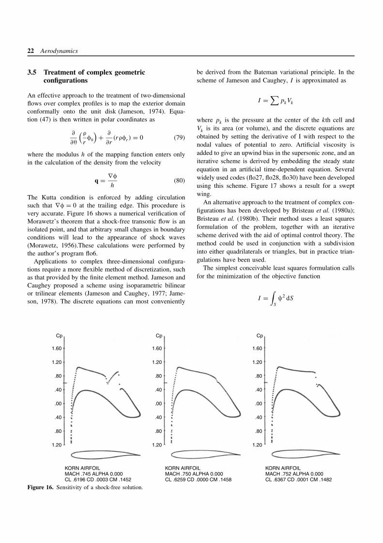
The Kutta condition is enforced by adding circulationsuch that ∇φ = 0 at the trailing edge. This procedure isvery accurate. Figure 16 shows a numerical verification ofMorawetz’s theorem that a shock-free transonic flow is anisolated point, and that arbitrary small changes in boundaryconditions will lead to the appearance of shock waves(Morawetz, 1956).These calculations were performed bythe author’s program flo6.
Applications to complex three-dimensional configura-tions require a more flexible method of discretization, suchas that provided by the finite element method. Jameson andCaughey proposed a scheme using isoparametric bilinearor trilinear elements (Jameson and Caughey, 1977; Jame-son, 1978). The discrete equations can most conveniently
be derived from the Bateman variational principle. In thescheme of Jameson and Caughey, I is approximated as
I =∑
pkVk
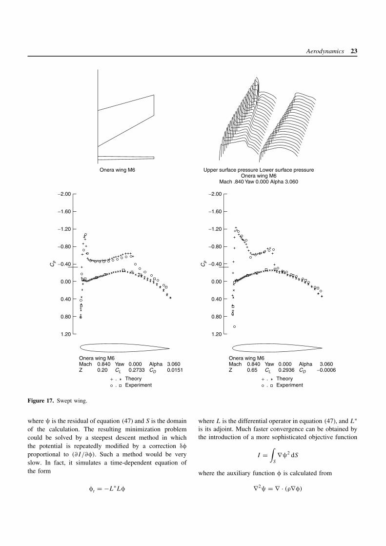
where pk is the pressure at the center of the kth cell andVk is its area (or volume), and the discrete equations areobtained by setting the derivative of I with respect to thenodal values of potential to zero. Artificial viscosity isadded to give an upwind bias in the supersonic zone, and aniterative scheme is derived by embedding the steady stateequation in an artificial time-dependent equation. Severalwidely used codes (flo27, flo28, flo30) have been developedusing this scheme. Figure 17 shows a result for a sweptwing.
An alternative approach to the treatment of complex con-figurations has been developed by Bristeau et al. (1980a);Bristeau et al. (1980b). Their method uses a least squaresformulation of the problem, together with an iterativescheme derived with the aid of optimal control theory. Themethod could be used in conjunction with a subdivisioninto either quadrilaterals or triangles, but in practice trian-gulations have been used.
The simplest conceivable least squares formulation callsfor the minimization of the objective function
I =∫
S
ψ2 dS
KORN AIRFOILMACH .752 ALPHA 0.000CL .6367 CD .0001 CM .1482
1.60
1.20
.40
.40
1.20
.80
.00
.80
Cp
KORN AIRFOILMACH .745 ALPHA 0.000CL .6196 CD .0003 CM .1452
.00
.40
1.60
1.20
.80
.80
.40
1.20
Cp
KORN AIRFOILMACH .750 ALPHA 0.000CL .6259 CD .0000 CM .1458
.40
1.60
1.20
.00
.80
.40
1.20
.80
Cp
Figure 16. Sensitivity of a shock-free solution.
Aerodynamics 23
−2.00
−1.60
−1.20
−0.80
−0.40
0.00
0.40
0.80
1.20
Cp
−2.00
−1.60
−1.20
−0.80
−0.40
0.00
0.40
0.80
1.20
Cp
Onera wing M6 Upper surface pressure Lower surface pressureOnera wing M6
Mach .840 Yaw 0.000 Alpha 3.060
Onera wing M6Mach 0.840 Yaw 0.000 Alpha 3.060Z 0.20 CL 0.2733 CD 0.0151
Onera wing M6Mach 0.840 Yaw 0.000 Alpha 3.060Z 0.65 CL 0.2936 CD −0.0006
. Experiment
. Theory. Experiment. Theory+ +
Figure 17. Swept wing.
where ψ is the residual of equation (47) and S is the domainof the calculation. The resulting minimization problemcould be solved by a steepest descent method in whichthe potential is repeatedly modified by a correction δφ
proportional to (∂I/∂φ). Such a method would be veryslow. In fact, it simulates a time-dependent equation ofthe form
φt = −L∗Lφ
where L is the differential operator in equation (47), and L∗is its adjoint. Much faster convergence can be obtained bythe introduction of a more sophisticated objective function
I =∫
S
∇ψ2 dS
where the auxiliary function φ is calculated from
∇2ψ = ∇ · (ρ∇φ)
24 Aerodynamics
Let g be the value of (∂φ/∂n) specified on the boundary C
of the domain. Then, this equation can be replaced by thecorresponding variational form∫
S
∇ψ · ∇v dS =∫
S
ρ∇ · ∇v dS −∫
C
gv dS
which must be satisfied by ψ for all differentiable testfunctions v. This formulation, which is equivalent to the useof an H−1 norm in Sobolev space, reduces the calculationof the potential to the solution of an optimal controlproblem, with φ as the control function and ψ as thestate function. It leads to an iterative scheme that calls
for solutions of Poisson equations twice in each cycle.A further improvement can be realized by the use of aconjugate gradient method instead of a simple steepestdescent method.
The least squares method in its basic form allows expan-sion shocks. In early formulations, these were eliminatedby penalty functions. Subsequently, it was found best touse upwind biasing of the density. The method has beenextended at Avions Marcel Dassault to the treatment ofextremely complex three-dimensional configurations, usinga subdivision of the domain into tetrahedra (Bristeau et al.,1985).