L07 Chapter 10 – Technology, Production, and Costs

Tech. Production, and Costs

Our familiar role in an economy

◦ Consumers

◦ Demand curves come from consumers

preferences

Today

◦ Producers, also known as firms

◦ Supply curves come mainly from costs of

production

◦ Firms make decisions like What to make? What inputs are required? What technique of

production will be used? How to structure compensation?

Technology – The process a firm uses to

turn inputs into outputs

◦ Lawn Mowing Example

Technological Change – change in in how

a firm uses its inputs

◦ Lawn Mowing – one person per lawn to

several people per lawn

Technology

Production

Classify into two general time periods

◦ Short run

A time period when at least one input is _______

Variable input = number of workers

Fixed input = size of the building

◦ Long run

A time period in which all inputs can change or be

varied

Number of workers can be changed ________

Size of building can be changed ________

_________is variable in long run!

Costs

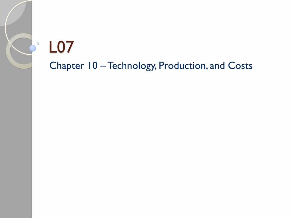
Total Cost = Fixed Costs + Variable Costs

TC = FC + VC

Total Cost

◦ The cost of all the inputs used in production

Variable costs

◦ Costs that change as output changes

Labor, Raw Materials, Electricity, Utilities

More firm produces, the more costs incurred

Fixed Costs

◦ Costs that remain the same as output changes

_______ does not change if you sell 1 pizza or 700 pizzas

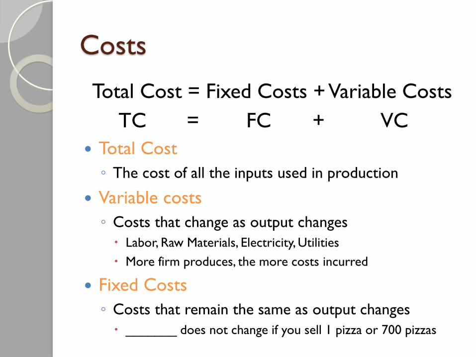
REMEMBER Economists always include opportunity costs!

Opportunity Cost: The highest valued alternative that must be given up to engage

in an activity

◦ Explicit Cost – A cost that involves spending money

◦ Implicit Cost – A nonmonetary opportunity cost

Costs

Economic

Profit

Implicit

Costs

Explicit

Costs

Accounting

Profit

Explicit

Costs

Revenue Revenue

Total

Economic

Costs

How an Economist

Views a Firm

How an Accountant

Views a Firm

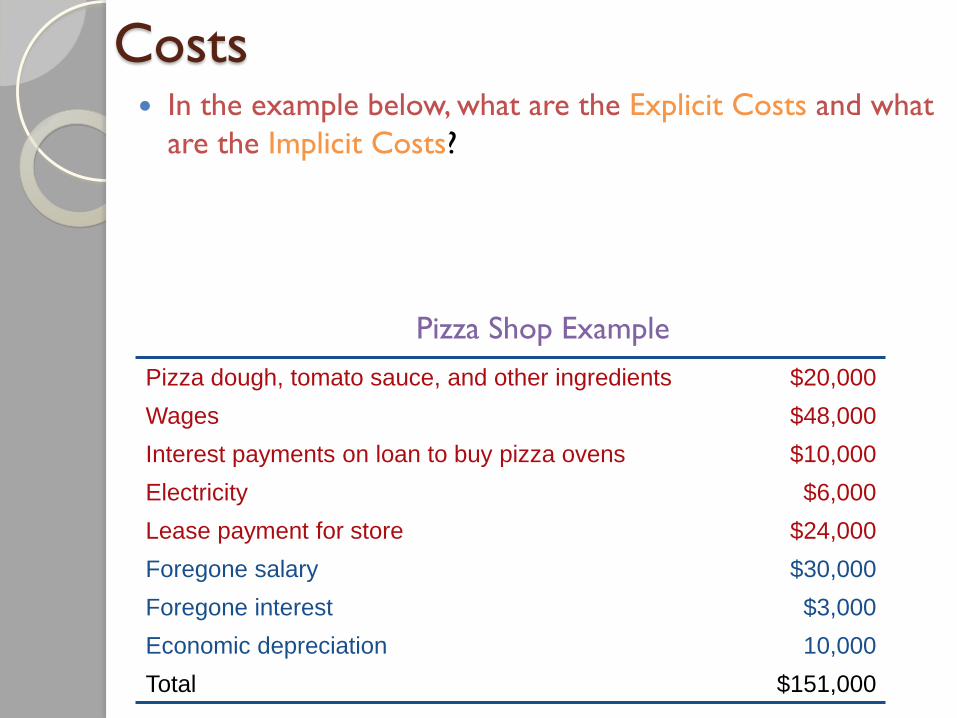
Costs In the example below, what are the Explicit Costs and what

are the Implicit Costs?

Pizza Shop Example

Pizza dough, tomato sauce, and other ingredients $20,000

Wages $48,000

Interest payments on loan to buy pizza ovens $10,000

Electricity $6,000

Lease payment for store $24,000

Foregone salary $30,000

Foregone interest $3,000

Economic depreciation 10,000

Total $151,000

Returns from hiring a worker

A firm has to pay a cost to hire a worker

◦ What does the firm receive in return?

◦ __________________________

200

450

550

600

625 640 Total Output

DQ4 from hiring fourth worker

DQ3 from hiring third worker

DQ2 from hiring second worker

DQ1 from hiring first worker

increasing marginal returns

diminishing marginal returns

Units of Output

Number of Workers 6 2 3 4 5 1

VARIABLE INPUT

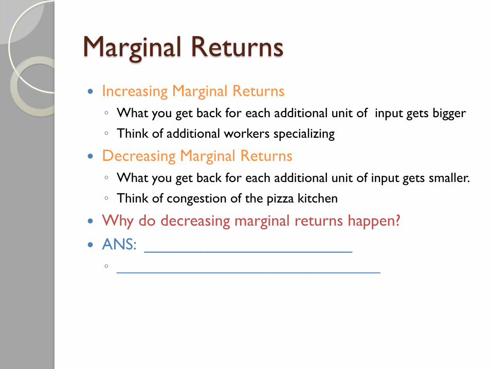
Marginal Returns

Increasing Marginal Returns

◦ What you get back for each additional unit of input gets bigger

◦ Think of additional workers specializing

Decreasing Marginal Returns

◦ What you get back for each additional unit of input gets smaller.

◦ Think of congestion of the pizza kitchen

Why do decreasing marginal returns happen?

ANS: _______________________

◦ ___________________________________

Marginal Product •Def: The Amount

added to total

output with each

additional worker

is called the

marginal Product

•How much did

the first worker

produce?

•____________

•How much

additional was

produced with 2

workers instead of

one?

•_____________

•Key Point:

•Marginal Product of Labor is

Upward sloping in the IMR region

• MPL is downward sloping in the

DMR region.

increasing marginal returns

diminishing marginal returns

Exam

Score in

History

Hours of Study 6 2 3 4 5 1

Example: History Exam Score

•Where is the region of

increasing marginal returns?

•__________________

•Where is the region of

diminish marginal returns?

•___________________.

•How do you see it?

•_______________________

________________________

_____________________

•_______________________

________________________

___________ 15

35

75

80

Costs

Next Step: Translate information about

inputs and outputs into information about

outputs and cost

Total Output

Units of Output

Number of Workers 6 2 3 4 5 1

650 1300

1950

2600

3250

3900

Units of Output

Total

Variable

Costs

Increasing

MR mean

Costs

increase

________

Decreasing MR mean Costs

increase _________

Each Unit

of Labor

costs

$650 per

week

200

450

550

600

625 640

200 450 550 600 625

640

IMR – Spreading Costs

of labor over more units

of output

650 1300

1950

2600

3250

3900

Units of Output

Variable

Costs Each Unit

of Labor

costs

$650 per

week

200 450 550 600 625

640

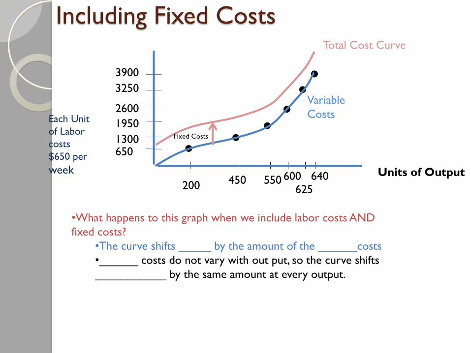
Total Cost Curve

•What happens to this graph when we include labor costs AND

fixed costs?

•The curve shifts _____ by the amount of the ______costs

•______ costs do not vary with out put, so the curve shifts

___________ by the same amount at every output.

Fixed Costs

Including Fixed Costs

Average vs. Marginal

Average always follows marginal

◦ Height Example

◦ GPA Example

If marginal is greater than average, then

the marginal unit pulls the average up.

If marginal is less than the average, then

the marginal unit drags the average down

650 1300

1950

2600

3250

3900

Units of Output

Costs

Each Unit

of Labor

costs

$650 per

week

200 450 550 600 625

640

•Marginal Cost – Additional Cost from producing on more unit of a good

•In the region of increasing marginal returns, marginal costs are falling

•This is because the firm is spreading additional cost over more

units

•In the region of decreasing marginal returns, marginal cost is rising

•This is because the firm is spreading additional cost over fewer

units

200 450 550 600 625

640

2

4

6

8

10

12

14

16

MC

ATC Costs

Total Cost Curve

Graphing Short Run Cost Curves THINGS TO NOTE

•Marginal cost curve

passes through the

minimum of ATC and AVC

•When MC is ______ATC

and AVC, MC is dragging

them _________.

•When MC is ______

ATC and AVC, MC is

pulling them _______

•Average Fixed Costs get

smaller with output.

•The distance between

ATC and AVC is AFC.

•Because AFC is getting

_________, the distance

between ATC and AVC

gets _______ too

Costs in the Long Run

What is different about the Long Run?

◦ Nothing is fixed

In long run:

◦ Total Cost and Average Cost curves have the same shape as in

the short run, but for different reasons

◦ In short run, the shapes were caused by increasing and

decreasing marginal returns.

◦ In the long run they are caused by Economies and Diseconomies

of Scale

◦ Economies of Scale – When a firm’s average costs fall as output

increases

Caused by:

Utilization of mass production

Purchasing inputs at lower cost because of their size

Costs in the Long Run

•Up to ___________, average costs

are decreasing Economies of

Scale

•Constant Returns to scale – LR

Average costs stay the same with

increasing output ___________

_________

•Diseconomies of scale: LR average

costs are increasing

•Caused by inability to manage

well such a large firm.

•Thought Experiment in the Long

Run:

•Choose the “plant size” to

minimize average costs

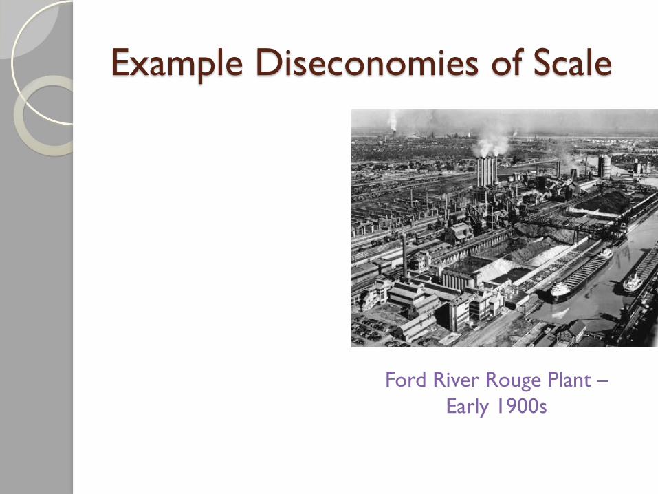
Example Diseconomies of Scale

Ford River Rouge Plant –

Early 1900s