Embed Size (px)
Citation preview

CHAPTER 11
QUASI-EXPERIMENTAL DESIGNS (Version 4, 14 March 2013) Page
11.1 ASSUMPTIONS UNDERPINNING OBSERVATIONAL STUDIES ............... 459
11.1.1. Problem Identification ...................................................................... 459
11.1.2. Delimiting the Statistical Population .............................................. 462
11.1.3. Random sampling ............................................................................ 464
11.1.4. Transient dynamics .......................................................................... 467
11.1.5. Predictions to be Tested .................................................................. 467
11.1.6. Relevant Variable Identification ...................................................... 468
11.2 TYPES OF QUASI-EXPERIMENTAL DESIGNS .......................................... 468
11.2.1. Designs without Control Groups .................................................... 469
11.2.2 Designs with Control Groups .......................................................... 471
11.3 ENVIRONMENTAL IMPACT DESIGNS ........................................................ 472
11.3.1 Types of Disturbances ...................................................................... 474
11.3.2 Transient Response Studies ............................................................ 477
11.3.3 Variability of Measurements ............................................................. 479
11.4 WHERE SHOULD I GO NEXT? .................................................................... 481
11.5 SUMMARY .................................................................................................... 482
SELECTED REFERENCES ................................................................................... 483
QUESTIONS AND PROBLEMS ............................................................................. 483
Much of the literature on experimental design has been driven by manipulative
experiments in which the investigator has the power to decide on the treatments to
be applied and the freedom to assign these treatments to experimental units in a
random manner. This aspect of experimental design was discussed in the previous
chapter. In this chapter we concentrate on the problems of experimental design as
applied to observational studies or mensurative experiments. Typically these are
field experiments in which the ‘treatments’ are already given by the environmental
mosaic. These types of studies are called quasi-experiments and they raise a set of

Chapter 11 Page 459
issues that are not faced in manipulative experimental studies (Shadish et al. 2002).
A quasi-experiment is defined as a study in which the treatments cannot be applied
at random to the experimental units. Many field experiments are quasi-experiments.
The aim of this chapter is to discuss the general principles of ecological
experimental design that qualify as quasi-experiments and the potential problems
they raise for scientific inference.
11.1 ASSUMPTIONS UNDERPINNING OBSERVATIONAL STUDIES
The key statistical problem that applies to all observational studies is that the
treatments are not under the control of the ecologist and randomization is restricted.
But there are an additional set of problems that are rarely discussed but are
particularly evident in observational studies. These problems are also relevant to
manipulative experiments that we discussed in the previous chapter.
All good ecology is founded on a detailed knowledge of the natural history of
the organisms being studied. The vagaries of species natural history are a challenge
to the field ecologist trying to understand natural systems as much as they are a
menace to modelers who assume that the world is simple and, if not linear, at least
organized in a few simple patterns. I begin with the often unstated background
supposition that we have good natural history information on the systems under
study. The great progress that ecology has made in the last century rests firmly on
this foundation of natural history. This background knowledge assists us in weighing
evidence from observational studies.
The following is a list of assumptions and decisions that are implicit or explicit
in every mensurative and manipulative experiment in ecology.
11.1.1. Problem Identification
This is a key step that is rarely discussed. A problem is typically a question, or an
issue that needs attention. Problems may be local and specific or general. Local
problems may be specific as to place as well as time, and if they are so constrained,
they normally are of interest to applied ecologists for practical management matters,
but are of little wider interest. General problems are a key to broader scientific
progress, and so ecologists should strive to address them to maximize progress.

Chapter 11 Page 460
The conceptual basis underpinning a study is an important identifier of a general
problem. Applied ecologists can often address what appear to be local problems in
ways that contribute to the definition and solution of general problems. A solution to
a general problem is what we call a general principle.
General ecological problems can be recognized only if there is sufficient
background information from natural history studies to know that an issue is broadly
applicable. There is also no easy way to know whether a general problem will be of
wide or narrow interest. For example, the general problem of whether biotic
communities are controlled from the top down by predation or from the bottom up by
nutrients is a central issue of the present time, and of broad interest (Estes et al.
2011). The answer to this question is critical for legislative controls on polluting
nutrients (Schindler 2006) as well as for basic fisheries management (Walters and
Martell 2004). The top-down/bottom-up issue will always be a general one for
ecologists to analyze because some systems will show top-down controls and
others bottom-up controls, so the answer will be case-specific. The level of
generality of the answer will not be “all systems are top-down,” but only some lower
level of generality, such as “Insectivorous bird communities are controlled bottom-
up.” It is only after the fact that problems are recognized as general, and science is
littered with approaches that once appeared to be of great general interest but did
not develop. The converse is also true: problems originally thought to be local have
at times blossomed into more general issues of wide relevance.

Chapter 11 Page 461
Example
Phosphorous controls primary
production in lakes
Some lakes limitedby micronutrients
General principle
Exceptions noted
Principle rejected Principle modified
Define more classes of lakes
Redefine classes of application
But most lakes are P limited
Figure 11.1. A schematic illustration of how generality is treated in ecological research. A simplified example from the controversy over the nutrients responsible for eutrophication in temperate freshwater lakes (Schindler 2006) is used to illustrate the progression from very general principles to more specific principles that are invariant. Statistical principles such as “primary productivity in 72% of freshwater lakes are controlled by phosphorus” are not very useful for management, and we try to reach universal principles (although we may never achieve this ideal).
The typical pattern in the evolution of general problems is illustrated in Figure
11.1. A problem is recognized, such as: What are the factors that control primary
production in lakes? From prior knowledge (e.g., agricultural research) or data from
a set of prior studies, a series of hypotheses is set up. A hypothesis that has a
reasonable amount of support is what we refer to as a general principle. One can
view these hypotheses as “straw men” in the sense that many variables affect any
ecological process, and all explanations should be multifactorial (Hilborn and
Stearns 1982). But it is not very useful at this stage to say that many factors are
involved and that the issue is complex. Ecologists should introduce complexity only
when necessary. Often it is useful to view a hypothesis as answering a practical
question: What variable might I change as a manager to make the largest impact on
the selected process? Ecologists should sort out the large effects before they worry
about the small effects. Large effects may arise from interactions between factors

Chapter 11 Page 462
that by themselves are thought to be of small importance. Good natural history is a
vital ingredient here because it helps us to make educated guesses about what
factors might be capable of producing large effects.
It is nearly universal that once a hypothesis is stated and some data are found
that are consistent with the suggested explanation, someone will find a contrary
example. For example, although most freshwater lakes are phosphorous-limited,
some are micronutrient-limited (e.g., by molybdenum; Goldman 1967; see also Elser
et al. 2007). The question then resolves into one of how often the original
suggestion is correct and how often it is incorrect, and one or another set of
hypotheses should be supported. Although statisticians may be happy with a
hypothesis that 87% of temperate lakes are phosphorous-limited, ecologists would
prefer to define two (or more) categories of lakes in relation to the factors limiting
primary production. We do this in order to produce some form of predictability for
the occasion when we are faced with a new lake: are there criteria by which we can
judge which factors might be limiting this particular lake? Can we establish criteria
that allow near-absolute predictability? Some might argue for a statistical cutoff,
such as 80% correct predictability, at which point we should be content with the
generalization. But the general approach of rigorous science is to concentrate on
those cases in which the prediction fails, so that by explaining contrary instances we
can strengthen the generalization.
11.1.2. Delimiting the Statistical Population
Ecologists often drive statisticians to distraction. We assume that place does not
matter, so that, for example, if we wish to study the predator/prey dynamics of
aphids and ladybird beetles on cabbage, we can do it anywhere that cabbage is
grown. Spatial invariance is a gigantic assumption, but a necessary one in the early
stages of an investigation in which we must assume simplicity until there is evidence
against it. This assumption about the irrelevance of the place or location where we
do our studies is often coupled with the assumption of time irrelevance, so we make
the joint assumption that our findings are independent of time and space.
Statisticians try to capture these assumptions in the idea of a “statistical population.”
Chapter 11 Page 463
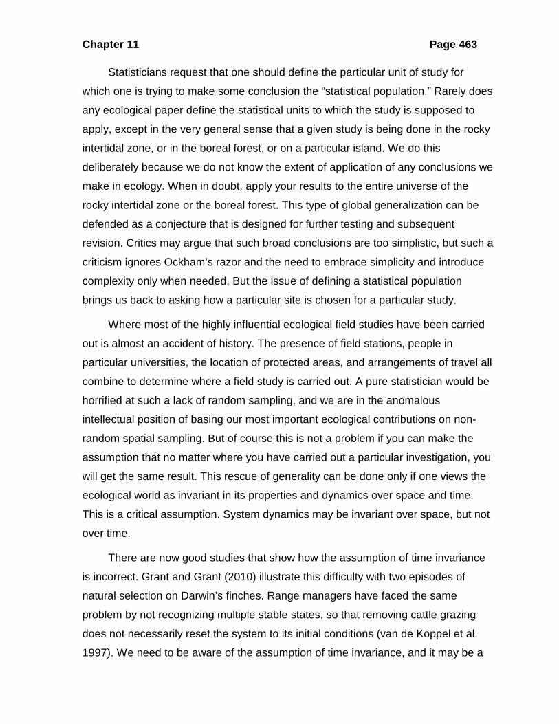
Statisticians request that one should define the particular unit of study for
which one is trying to make some conclusion the “statistical population.” Rarely does
any ecological paper define the statistical units to which the study is supposed to
apply, except in the very general sense that a given study is being done in the rocky
intertidal zone, or in the boreal forest, or on a particular island. We do this
deliberately because we do not know the extent of application of any conclusions we
make in ecology. When in doubt, apply your results to the entire universe of the
rocky intertidal zone or the boreal forest. This type of global generalization can be
defended as a conjecture that is designed for further testing and subsequent
revision. Critics may argue that such broad conclusions are too simplistic, but such a
criticism ignores Ockham’s razor and the need to embrace simplicity and introduce
complexity only when needed. But the issue of defining a statistical population
brings us back to asking how a particular site is chosen for a particular study.
Where most of the highly influential ecological field studies have been carried
out is almost an accident of history. The presence of field stations, people in
particular universities, the location of protected areas, and arrangements of travel all
combine to determine where a field study is carried out. A pure statistician would be
horrified at such a lack of random sampling, and we are in the anomalous
intellectual position of basing our most important ecological contributions on non-
random spatial sampling. But of course this is not a problem if you can make the
assumption that no matter where you have carried out a particular investigation, you
will get the same result. This rescue of generality can be done only if one views the
ecological world as invariant in its properties and dynamics over space and time.
This is a critical assumption. System dynamics may be invariant over space, but not
over time.
There are now good studies that show how the assumption of time invariance
is incorrect. Grant and Grant (2010) illustrate this difficulty with two episodes of
natural selection on Darwin’s finches. Range managers have faced the same
problem by not recognizing multiple stable states, so that removing cattle grazing
does not necessarily reset the system to its initial conditions (van de Koppel et al.
1997). We need to be aware of the assumption of time invariance, and it may be a

Chapter 11 Page 464
mistake to assume that, if a particular study was done from 1970 to 1980, the same
results would have been observed from 2001 to 2011.
The assumption of spatial invariance (Pulliam and Waser 2010), has never
been popular in ecology because the abundance of resources, predators, and
diseases are well known to vary spatially. Much of modern ecology has focused on
trying to explain spatial variation in processes. The exact dynamics of a community
may be greatly affected by the species present, their interaction strengths, and their
relative abundances. We do not yet know how much variation can occur in
community composition before new rules or principles come into play.
The result is that we almost never specify a statistical population in any
ecological research program, and we issue a vague statement of the generality of
our findings without defining the units to which it should apply. This is not a problem
in experimental design if we can repeat our findings in another ecosystem to test
their generality. The key to generality is to predict correctly what we will find when
we study another ecological system in another place.
11.1.3. Random sampling
In the chosen area of study, ecologists observe or apply some treatments to obtain
the data that will test an array of alternative hypotheses. In the case of observational
experiments the sample units are defined by nature, and our job in random sampling
is to locate them, number them, and select those for treatment at random. For
manipulative experiments, as discussed in the last chapter, we define the sample
units and apply a similar random selection of them for each treatment. Most
ecological field experiments have a small number of replicates, and Hurlbert (1984,
see Figure 10.3 page 430) has discussed what can happen if treatments are defined
randomly. All our control or experimental plots may end up, for example, on north-
facing slopes. Hurlbert (1984) recommended maintaining an interspersion of
treatments so that both treatments and controls are spread spatially around the
study zone, a recommendation for non-random spatial sampling.
Consequently a good biologist almost never follows the instructions from the
pure statistician for three reasons. First, they may not be practical. The major reason

Chapter 11 Page 465
such random assignments may not be practical is that transportation to the sites
may limit choices. Not everyone can access field sites by helicopter, and roads
typically determine which study units can be used. Table 11.1 gives one example of
the kinds of problems ecologists face in delimiting experimental units in a field
situation. Second, places for study may need to be in a protected nature reserve or
an area in which the private owner welcomes ecologists to use his or her land. Since
nature reserves in particular are often put in landscapes that cannot be used
economically for agriculture or farming, there is an immediate bias in the location of
our experimental units. Third, field stations or other sites where research has been
carried out in the past have a legacy of information that draws ecologists to them for
very good reasons (Aigner and Kohler, 2010, although this compounds the spatial
nonrandomness of choice of field sites.
.

Chapter 11 Page 466
Table 11.1. Experimental manipulations in the Kluane Boreal Forest Ecosystem Project and the decisions that led to their site placement. Each experimental unit was 1 km2. This example illustrates some of the reasons randomization cannot be achieved in field ecology. Similar forested habitat was the first constraint on area selection, and access in summer and winter was the secondary determinant of location, followed by the need to spread treatments over the 350 km2 study area. Details are given in Krebs et al. (2001).
Experimental unit Treatment Reasons for location Fertilizer 1 55 tons of commercial fertilizer
added aerially each year Along Alaska Highway at north end of study area, 3 km from airstrip used for aircraft loading fertilizer
Fertilizer 2 55 tons of commercial fertilizer added aerially each year
Along Alaska Highway near north end of study area, 6 km from airstrip, separated from other treatments by at least 1 km
Food addition 1 Commercial rabbit chow fed year round
Access by ATV in summer and minimum 1 km spacing from electric fence treatment
Food addition 2 Commercial rabbit chow fed year round
At extreme southern end of study area with ATV access and 3 km from Control 3
Electric fence Exclude mammal predators Along Alaska Highway, access by heavy equipment, relatively flat area Electric fence and food addition
Exclude mammal predators and add rabbit chow food
Near Alaska Highway, access by heavy equipment, one side of fence already cleared for old pipeline, relatively flat area
Control 1 None Along Alaska Highway, spaced 1 km from manipulated areas and 10 km from Control 2
Control 2 None Along Alaska Highway, spaced 5 km from Control 3 and 7 km from nearest treatment site
Control 3 None Near southern end of study area accessed by old gravel road

Chapter 11 Page 467
The consequence of these problems is the practical advice to randomize when
possible on a local scale, and to hope that generality can emerge from nonrandom
sampling on a regional or global scale
11.1.4. Transient dynamics
The time scale of ecological system responses is assumed to lie within the time
frame of our studies. Thus, if we manipulate vole or lemming populations that have
several generations per year, we assume that our manipulations will be effective within
a year. But what if fast variables like vole numbers interact with slow variables like soil
nutrient dynamics or climate change? Or what if we are studying species like whales
that can live for 100 years or more?
The time lags in system response that are inherent in transient dynamics can be
found only by longer-term studies (e.g., Grant and Grant, 2010), and at present we are
guided in these matters only by our intuition, which is based on natural history
knowledge and process-based (i.e., mechanistic) models that can explore our
assumptions about system dynamics. Process-based models are a vital component of
our search for generality because they can become general principles waiting for further
testing (e.g., see King and Schaffer 2001; Pulliam and Waser, 2010). The important
limitation of process-based models is to determine how much structure is essential to
understanding the system of study. Too much detail leaves empirical scientists with little
ability to discern which factors are more important, and too little detail leaves out
biological factors that are critical.
11.1.5. Predictions to be Tested
Ecological hypotheses typically are less clearly structured logically than might be
desirable. In particular the background assumptions that are necessary to support
deductions from a particular hypothesis are rarely stated, with the net result that there is
a somewhat tenuous connection between hypotheses and predictions. Verbal models
are particularly vulnerable on this account. Part of the answer is to specify quantitative
models and the danger here is to be overly precise and multiply parameters excessively

Chapter 11 Page 468
(Ginzburg and Jensen 2004. One remedy for this problem is to demand more rigor in
specifying the unstated assumptions that accompany every study.
11.1.6. Relevant Variable Identification
Another difficulty at this stage is that the set of alternative hypotheses proposed as
explanations of the identified problem may not include the correct explanation. For
example, the three alternative hypotheses for freshwater lakes—that primary production
is limited by nitrogen, phosphorus, or carbon—may all be wrong if a lake’s production is
limited by micronutrients such as molybdenum. There is no simple way out of this
problem, except to identify as wide an array of possible explanations as current
knowledge will permit, and to recognize always that in the future a new hypothesis may
arise that we had not considered.
By diversifying one’s observations at a variety of places, we can minimize the
probability of failing to see and include a relevant variable. Diversifying means carrying
out similar studies in several different places. This is one of the strongest
recommendations that one can make about ecological science: we should
systematically diversify our observations in different places to help identify relevant
variables. If we have missed an important variable, it will be picked up when
management actions flow from our ecological findings, because those actions will not
achieve their predicted results. Practical management can be used as the touchstone of
ecological ideas and as a valuable test for missing variables. This will occur only when
management actions have a firm foundation in ecological ideas and—if management
actions fail—when time and money are made available to find the source of the failure.
Ignoring failures of predictions is a sure way to reduce progress in scientific
understanding (Popper 1963).
11.2 TYPES OF QUASI-EXPERIMENTAL DESIGNS
The social sciences have contributed extensively to discussions about the problems of
quasi-experimental designs (Shadish et al. 2002), but the issue of experimental design
has also been a focus of applied ecologists (e.g. Hone 2007, Anderson et al. 2001,
Johnson 2002). In this section I will discuss two general types of quasi-experimental
designs and their assumptions and limitations. For all these designs the discussions

Chapter 11 Page 469
about treatment structure, design structure, and response structure from Chapter 10
apply.
11.2.1. Designs without Control Groups
In some cases of ecological and social science research there can be no control group.
The most highly visible ecological problem of our day is the impact of climate change on
ecosystems, since we have only one Earth that is changing. Designs without control
groups face a difficult problem of inference and of course should be avoided if at all
possible. But the problem is that ecologists are often called upon for information about
environmental impacts that they do not control the timing of.
Figure 11.2 illustrates the types of designs that ecologists can use without control
groups. Hone (2007) labeled scientific studies without controls pseudo-experiments to
point out the difficulties of achieving reliable inference without control groups.
Design Time sequence
One-group Post-treatment observations:Treatment Observe / Measure
One-group Pre- and Post-treatment observations:Observe / Measure Treatment Observe / Measure
Removed Treatment design:Observe / Measure Treatment Observe / Measure No treatment Observe / Measure
Repeated Treatment design:Observe / Measure Treatment Observe / Measure Observe / Measure Treatment Observe / Measure Figure 11.2. Schematic illustration of four types of quasi-experimental designs without controls. The strength of inference increases from the top to the bottom of the table. The term ‘treatment’ refers to the ecological process of interest and typically is a situation in nature rather than a manipulated variable. For example, a ‘treatment’ could be a forest fire. (Modified after Shadish et al. 2002, Table 4.1.)
11.2.1.1 One-group Post-treatment design
This is a very weak design in which some ecological event has occurred like a forest fire
and the only observations or measurements we have are after the event. The major
weakness is that we try to infer treatment = cause and observations = effect from this
design but we do not know if historical factors that preceded the treatment are the true
cause of the observed measurements or that this is simply a time trend. This design

Chapter 11 Page 470
can be useful in situations with a strong observational or theoretical background and
good knowledge of the particular ecological system. But do not stake your reputation on
the outcome of these kinds of studies because they are far from strong inference.
11.2.1.2 One-group Pre- and Post-treatment observations
It is possible to strengthen this type of design with no controls if data are available on
the site before the treatment occurs. To achieve valid inference we have to assume
there are no transient or permanent time effects that affect the resulting data and no
change in the experimental units from other confounding causes. In many cases if short
time periods are involved, these problems might be minimized.
Another way to strengthen this type of design is to make two or more periods of
measurement before the treatments is imposed. This design allows you to determine
the stability of the measurements over time when no treatment is yet imposed. If there
is high variability in your measurements, this would make it very difficult to detect a
significant effect unless the effect is very large.
11.2.1.3 Removed and Repeated Treatment Designs
In some cases in which there is some control over the treatment, it is possible to
combine the previous design of observations-treatment-observations with a follow-up
(while the treatment is still being applied) of an additional observation-removal of
treatment-observation design. The principle is that if the treatment affects the
measurements positively (for example), then the following removal of the treatment
should affect the measurements negatively (for this example). Figure 11.3 illustrates the
general principle of this design.
With these designs it is useful to make observations or measurements at equally
spaced time intervals to get rates of change. If the treatment does not have permanent
effects on the ecological system, it may be possible to repeat the treatment at second
time (Figure 11.3b). But if the treatment induces transient dynamics into the ecological
system, the timing of the repeat treatment will be critical since one has to wait until the
system settles down to its previous level (if this ever occurs).

Chapter 11 Page 471
The bottom line is that it is possible to obtain reliable information from
observational experiments in which there is no control possible, but the possible pitfalls
are many and the knowledge gained by such experiments should be considered
tentative and exploratory rather than definite.
Time
0 1 2 3 4 5 6 7 8 9
Mea
sure
men
t
0.0
0.2
0.4
0.6
0.8
1.0
PRE-TREATMENT
TREATMENT TREATMENT
(b)
NOTREATMENT
Time
0 1 2 3 4 5 6 7 8 9
Mea
sure
men
t
0.0
0.2
0.4
0.6
0.8
1.0PRE-
TREATMENT
TREATMENT
TREATMENTREMOVED
(a)
Figure 11.3. Schematic illustration of two ways of strengthing quasi-experimental designs without controls. (a) The removed treatment design with one possible outcome of a mensurative experiment. (b) The repeated treatment design with the addition of a second set of treatments and observations in which you can look for a repeat in the measured effect.
11.2.2 Designs with Control Groups
Adding a control group that receives no treatment is one method of strengthening the
inferences from quasi-experimental designs. The problem with many ecological field
experiments is that the control group can not be randomly assigned. While it is feasible
in some cases in which we control the treatments to assign treatments at random to
experimental units, too often in field ecology we cannot do this because the ‘treatments’
Chapter 11 Page 472
are a product of geology, recent history such as fires, human activities such as mining
operations, or on a larger scale evolution.
There are two simple versions of these designs. In the first case, we have no
observations on the treatment group before the treatment occurred, and we compare
our measurements within the treated group or region with equivalent measurements
made on groups or a region that was not subject to the ‘treatment’. For example, we
might compare the biodiversity of plants in two areas, one subject to fire at some time
prior to our study and a second area where fire has not occurred on the time scale of
interest. To make a statistical test of these kinds of data, you must assume that the two
areas differ only in their fire history, a somewhat dubious assumption in many
circumstances.
A stronger version of this approach occurs when we have data from the areas
before the ‘treatment’ occurred. This is possible only when the treatment can be carried
out by the experimenter or if it is due to human activity, when advance warning of an
environmental change is given, as when a mine or a pipeline is planned in an area.
These kinds of quasi-experimental designs meld into an important area in applied
ecology, environmental impact studies. The designs for impact studies have been
discussed extensively by ecologists and they typically suffer from many of the problems
of quasi-experimental designs that we discussed above.
11.3 ENVIRONMENTAL IMPACT DESIGNS
Environmental impact studies form an important component of applied ecological
research and it is important that these studies be done properly. These studies are
called interrupted time series designs in the social science literature (c.f. Shadish et al.,
2006, Chapter 6). The basic idea is that a series of measurements are taken in time
and at some point a treatment or intervention is applied, after which more
measurements are taken. There may or may not be a change in the time series after
the intervention, and this could take the form of an abrupt change as illustrated in
Figure 11.4 or a change in the slope of the time series data. Changes may be
immediate or delayed, and special statistical methods are needed to treat these kinds
of interrupted time series.

Chapter 11 Page 473
The basic types of environmental impact studies have been summarized by Green
(1979) and are illustrated in Figure 11.4 Populations typically vary in abundance from
time to time, and this variability or ‘noise’ means that detecting impacts may be difficult.
By replicating measurements of abundance several times before the anticipated impact
and several times after you can determine statistically if an impact has occurred (Fig.
11.4a). If there is only one control area and one impact area, all differences will be
attributed to the impact, even if other ecological factors may, for example, affect the
control area but not the impact area. For this reason Underwood (1994) pointed out that
a spatial replication of control sites is also highly desirable (Fig. 11.4b). Note that the
different control sites may differ among themselves in average population abundance
because of habitat variation. This variation among areas can be removed in an analysis
of variance, and the relevant ecological measure is whether the impact area changes
after the impact, relative to the controls. This will show up in the analysis of variance as
a significant interaction between locations and time and should be obvious visually as
shown in Figure 11.4.

Chapter 11 Page 474
(a) Temporal replication
Time - months
0 5 10 15 20
Mea
n ab
unda
nce
2
3
4
5
6
Control area
Impact area
(b) Temporal and spatial replication
Time - months
0 5 10 15 20
Mea
n ab
unda
nce
2
3
4
5
6
Control area 1
Impact areaControl area 2
Control area 3
Figure 11.4 Environmental impact assessment using the BACI quasi-experimental design (Before-After, Control-Impact). The abundance of some indicator species is measured several times before and after impact (indicated by arrow). The statistical problem is to determine if the changes in the impact zone represent a significant changes in abundance or merely random variations in abundance. (a) The simplest design with one control site and one impact site. (b) By adding spatial replication to the design, unique changes on one control site can be recognized and the power of the ecological inference increased.
11.3.1 Types of Disturbances
It is useful to distinguish two different types of environmental disturbances or
experimental perturbations. Pulse disturbances occur once and then stop. Press
disturbances continue to occur and because they are sustained disturbances they
ought to be easier to detect. Under press disturbances an ecological system ought to
reach an equilibrium after the initial transition changes, assuming simple dynamics.

Chapter 11 Page 475
Pulse disturbances may also produce ecological effects that are long term, even if the
actual disturbance itself was short. A flood on a river or a fire in a forest are two
examples of pulse disturbances with long-term impacts. A supplemental feeding
experiment could be a press experiment in which feeding is continued for several
months or years, or it could be a pulse experiment in which food is added only once to
a population. Pulse disturbances typically generate transient dynamics so that the
ecological system may be changing continuously rather than at an equilibrium.
Transient dynamics occur on different time scales for different species and
communities and can be recognized by time trends in the data being measured.
Disturbances may change not only the average abundance of the target
organisms but also the variability of the population over time. In many populations the
variability of a population is directly related to its abundance so that larger populations
will have larger temporal variances. Decisions must be made in any impact assessment
about the frequency of sampling. If samples are taken too infrequently, pulse
disturbances could go undetected (Underwood 1994). The time course of sampling is
partly determined by the life cycles of the target organisms, and there will be for each
ecological system an optimal frequency of sampling. If you sample too frequently, the
observed abundances are not statistically independent. The conclusion is that impact
assessment must be highly species- and habitat-specific in its design.
Statistical tests for impact studies are discussed in detail by Stewart-Oaten et al.
(1992) and Underwood (1994). Many impact assessments use randomization tests to
measure changes at impact sites (Carpenter et al. 1989).
Randomization tests are similar to t-tests in measuring differences between
control and impact sites:
ˆˆ ˆt t td C I= − (11.1)
where ˆ Estimated difference in the ecological variable of interest at time ˆ Value of the variable on the control site at time ˆ Value of the variable on the impact site at time
t
t
t
d tC tI t
===

Chapter 11 Page 476
A two-sample t test would compare these dt values before and after the impact. A
randomization test would compare the average d value before and after the impact with
a series of random samples of all the d-values regardless of their timing. Both of these
tests assume that the successive d-values are independent samples, that variances are
the same in the control and impact populations, and that the effects of the impact are
additive. Stewart-Oaten et al. (1992) discuss the implications of the violation of these
assumptions which can render the formal statistical tests invalid. A simple illustration of
these methods is shown in Box 11.1.
Box 11.1 USE OF THE WELCH T-TEST AND THE RANDOMIZATION TEST TO ASSESS ENVIRONMENTAL IMPACTS IN A BACI DESIGN (BEFORE-AFTER CONTROL-IMPACT).
Estimates of chironomid abundance in sediments were taken at one station above and one below a pulpmill outflow pipe for three years before plant operation and for 6 years after with the following results: Year Control site Impact site Difference
(control-impact)
1988 14 17 -3 1989 12 14 -2 1990 15 17 -3 Impact begins 1991 16 21 -5 1992 13 24 -11 1993 12 20 -8 1994 15 21 -6 1995 17 26 -9 1996 14 23 -9 We analyze the differences between the control and impact sites. Using B for the before data and A for the after impact data and the usual statistical formulas we obtain:
( )
2
23, 2.67, 0.336, 8.00, 4.80
Estimated difference due to impact = 2.67 8.00 5.33
B B B
A A A
B A
n d sn d s
d d
= = − == = − =
− = − − − =
Compute Welch’s t-test as described in Zar (2010, p. 129) or Sokal and Rohlf (2012, page 404) as:

Chapter 11 Page 477
( )2 2
2.67 8.00 5.33 5.590.33 4.80 0.9111
3 6
B A
B A
B A
d dts sn n
− − −−= = = =
++
Because the Welch test allows for unequal variances before and after impact, the degrees of freedom are adjusted by the following formula from Zar (2010, p. 129):
( )( ) ( )
22 2
2
2 2 2 22 2
0.9111. . 6.19 (rounded to 6)
0.111 0.802 5
1 1
B A
B A
B A
B A
B A
s sn n
d fs sn n
n n
+
= = =
+ +
− −
The critical value from Student’s t-distribution for 6 degrees of freedom at α = 0.05 is 2.447 and consequently we reject the null hypothesis that chironomid abundance is not impacted by the pulpmill effluent. These data can also be analyzed by a randomization test (Sokal and Rohlf 2012, pg. 803). Randomization tests are computer intensive, but are simple in principle and proceed as follows: 1). All the 9 difference values are put into a hat and random samples of n=3 are
drawn to represent the Before data and n=6 to represent the After data. This sampling is done without replacement.
2). This procedure is repeated 500-1000 times or more in a computer to generate a distribution of difference values that one would expect under the null hypothesis of no difference in the before-after abundance values. Manly (1991) provides a computer program to do these computations.
3). For these particular data, a randomization test of 5000 samples gave only 1.32% of the differences equal to or larger than the observed -5.33 difference in mean abundance. We would therefore reject the null hypothesis of no impact.
This example is simplified by having only one control and one impact site. If several control sites are used, as recommended for increased power, ANOVA methods should be used as described by Underwood (1994, pg. 6).
Environmental impact designs work well if the effect of the applied treatment
occurs rapidly, but in some cases the impact is delayed in time so that a short-term
study may well conclude that no effect has occurred. Knowledge of the mechanisms of
response to the particular impact is critical for assessing whether or not delayed
changes could be expected. If short-term decision-making is enforced the possibility of
detecting significant long-term trends will be missed.
Chapter 11 Page 478
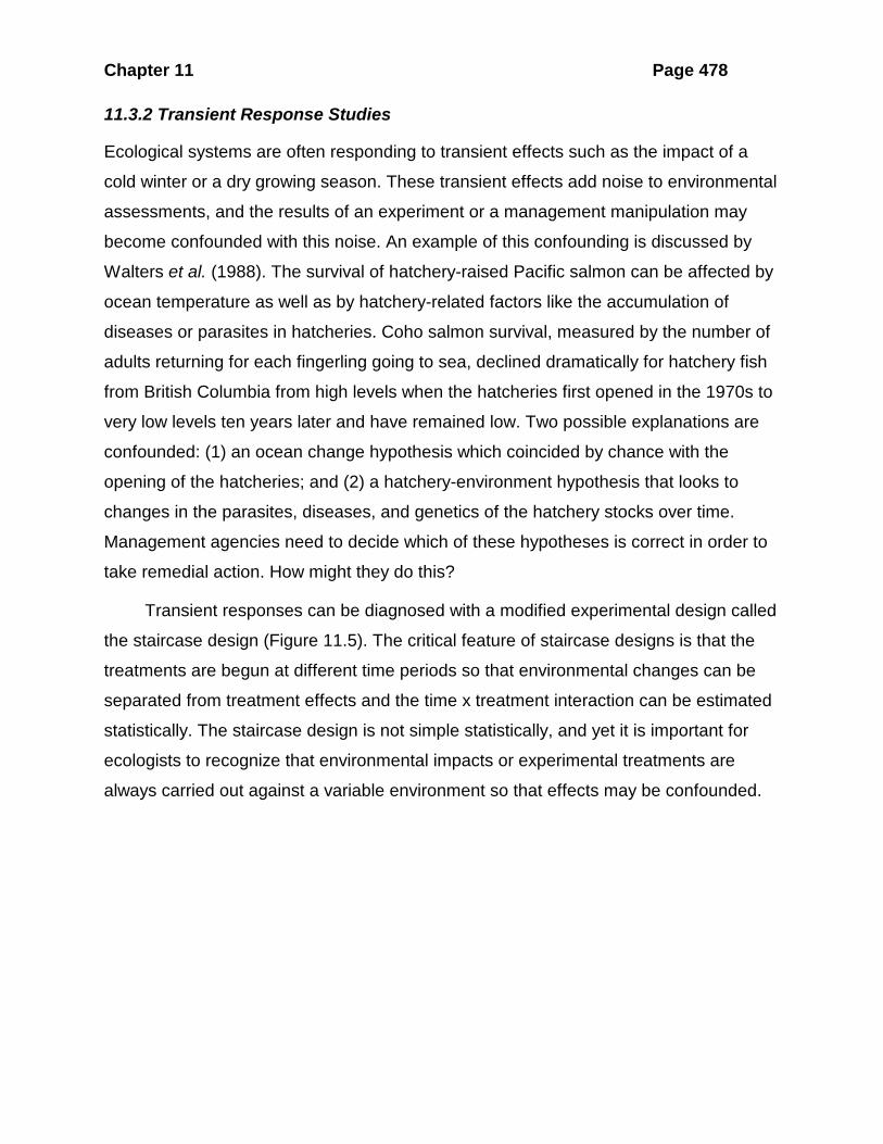
11.3.2 Transient Response Studies
Ecological systems are often responding to transient effects such as the impact of a
cold winter or a dry growing season. These transient effects add noise to environmental
assessments, and the results of an experiment or a management manipulation may
become confounded with this noise. An example of this confounding is discussed by
Walters et al. (1988). The survival of hatchery-raised Pacific salmon can be affected by
ocean temperature as well as by hatchery-related factors like the accumulation of
diseases or parasites in hatcheries. Coho salmon survival, measured by the number of
adults returning for each fingerling going to sea, declined dramatically for hatchery fish
from British Columbia from high levels when the hatcheries first opened in the 1970s to
very low levels ten years later and have remained low. Two possible explanations are
confounded: (1) an ocean change hypothesis which coincided by chance with the
opening of the hatcheries; and (2) a hatchery-environment hypothesis that looks to
changes in the parasites, diseases, and genetics of the hatchery stocks over time.
Management agencies need to decide which of these hypotheses is correct in order to
take remedial action. How might they do this?
Transient responses can be diagnosed with a modified experimental design called
the staircase design (Figure 11.5). The critical feature of staircase designs is that the
treatments are begun at different time periods so that environmental changes can be
separated from treatment effects and the time x treatment interaction can be estimated
statistically. The staircase design is not simple statistically, and yet it is important for
ecologists to recognize that environmental impacts or experimental treatments are
always carried out against a variable environment so that effects may be confounded.

Chapter 11 Page 479
1 102 3 4 5 6 7 8 9YEAR
Control
Stream # 1
Stream # 2
Stream # 3
Stream # 4
B
B
B
B
Figure 11.5 Staircase design for environmental impact studies in which environmental time trends may confound treatment effects. In this example, all salmon streams are monitored for at least one year before a hatchery is operated at point B, and the four hatcheries begin operation in four successive years. (Modified from Walters et al. 1988)
11.3.3 Variability of Measurements
The power of any test for environmental impacts is constrained by the variability of the
data being gathered, the magnitude of the environmental impact, and the number of
replicates obtained in time and space. The choice of the type of data to be gathered is
the first choice in any ecological study, and we need to know the variability to design
powerful impact studies. Osenberg et al. (1994) considered three types of data that
might be gathered - physical-chemical data (e.g. temperature, nutrient concentrations),
individual-based data (e.g. body size, gonad weight, condition), and population-based
measures (e.g. density). Individual and population data can be gathered on many
different species in the community. Osenberg and Schmitt (1994) provide an interesting
data set for a marine study, and provide a model for the kind of approach that would be
useful for other impact studies. First, they measured impacts as the difference in the
parameter between the control site and the impact site at a specific time (eq. 11.1
above). Population based parameters were most highly variable (Figure 11.6a) and
physical chemical parameters were least variable. All else being equal, physical-
chemical parameters should provide more reliable measures of environmental impact.

Chapter 11 Page 480
But a second critical variable intervenes here - the effect size, or how large a change
occurs in response to the impact. For this particular system Figure 11.6b shows that the
effect size is much larger for population parameters than for chemical parameters.
Standardized Effect Size
Stan
dard
ized
effe
ct s
ize
0.0
0.2
0.4
0.6
0.8
1.0
1.2
1.4
Chemical-physical
Individual Population
(c)
Absolute Effect Size
Effe
ct s
ize
0.0
0.2
0.4
Chemical-physical
Individual Population
(a)
(b)
Temporal Variability
Varia
bilit
y
0.0
0.2
0.4
0.6
0.8
1.0
Chemical-physical
Individual Population
Figure 11.6 Estimates of parameter variability for a California marine coastal environmental impact study. All measures of variables refer to the differences between control and impact sites (eq. 11.1). (a) Temporal variability for 30 chemical-physical variables, 7 individual-based variables, and 25 population-based variables. (b) Absolute effect sizes (mean difference before and after) to measure the impact of the polluted water on chemical-physical, individual-, and population-based variables. (c) Standardized effect sizes which combine (a) and (b) for these variables. Variables with larger standardized effect sizes are more powerful for monitoring impacts. (Data from Osenberg et al. 1994).
By combining these two measures into a measure of standardized effect size we can
determine the best variables statistically:
absolute effect sizeStandardized effect sizestandard deviation of differences
B A
d
d ds
=
−=
(11.2)

Chapter 11 Page 481
where
Mean difference between sites before impact beginsMean difference between sites after impact beginsStandard deviation of observed differences between sites
B
A
d
dds
===
Figure 11.6c shows the standardized effect sizes for this particular study. Individual-
based parameters are better than either physical-chemical or population-based
measures for detecting impacts. Approximately four times as many samples would be
needed to detect an impact with population-based measures, compared with individual-
based measures.
This example must not be generalized to all environmental impact assessments
but it does provide a template of how to proceed to evaluate what variables might be
the best ones to measure to detect impacts. It emphasizes the critical point in
experimental design that measurements with high variability can be useful indicators if
they also show large effect sizes. What is critical in all ecological research is not
statistical significance but ecological significance which is measured by effect sizes.
How large an impact has occurred is the central issue, and “large” can be defined only
with respect to a specific ecosystem.
11.4 WHERE SHOULD I GO NEXT?
Many ecological field studies must use quasi-experimental designs in which the
‘treatments’ are specified by geography, geology, or disturbances like fires. The thrust
of this chapter is to outline briefly the problems that arise with quasi-experimental
designs and the limitations they impose on scientific inference. Once these are
recognized, many field studies can be fitted into the analysis framework of experimental
design discussed for manipulative experiments in the previous chapter. Critical thinking
in quasi-experiments means showing that the alternative hypotheses are unlikely. This
type of approach to ecological experiments is akin to that suggested by Popper (1963)
who suggested that it was more useful in science to try to reject hypotheses rather than
confirming them. The problem with quasi-experiments is that arguments for rejection
may be weak.

Chapter 11 Page 482
The social and medical sciences in which the experimental units are human
beings have discussed the problems of quasi-experimental designs in extensive detail,
and students are referred to Shadish et al. (2002) for extended discussion on these
issues. Many of these issues arise in management studies of policies for fishing and
hunting regulations, water quality analysis, or pest control alternatives (Manly 2001).
11.5 SUMMARY
In many ecological studies the process of interest cannot be manipulated so that one
must do observational studies, ‘natural experiments’, or mensurative experiments. The
fundamental limitation is that the ‘treatments’ cannot be assigned randomly, and we
recognize this by calling such studies quasi-experiments. Such experiments seek to
understand cause and effect in the same manner as manipulative experiments but face
the difficulty that the ‘treatment’ units may have no suitable controls for comparison.
Even if controls exist for the study design, the issue of how comparable the controls are
to the ‘treatments’ must be considered.
Social scientists have made considerable progress in dealing with the problems
raised by the inability to assign treatments at random to experimental units and the
failure to select experimental units at random. Some of these techniques are useful in
ecological quasi-experiments as we try to identify the causal structure of ecological
processes. Ecologists would like their conclusions to be spatial-invariant and time-
invariant but this is difficult to achieve because of heterogeneity in both these
dimensions.
Environmental impact studies present design problems identical to those of any
ecological quasi-experiment and are called interrupted time series designs. The BACI
(Before-After Control-Impact) design provides a mechanism for analyzing impacts if it
can be implemented. If environmental time trends occur they may be confounded with
experimental impacts unless care is taken to provide temporal replication. Different
variables can be measured to assess impacts and some provide more statistical power
than others.

Chapter 11 Page 483
SELECTED REFERENCES
Bråthen, K.A., et al. 2007. Induced shift in ecosystem productivity? Extensive scale effects of abundant large herbivores. Ecosystems 10: 773-789.
Hone, J. 2007. Wildlife Damage Control. CSIRO Publishing, Collingwood, Victoria. 179 pp.
Manly, B.F.J. 2001. Statistics for Environmental Science and Management. Chapman and Hall, New York. 326 pp.
Martin, J.-L., Stockton, S., Allombert, S., and Gaston, A. 2010. Top-down and bottom-up consequences of unchecked ungulate browsing on plant and animal diversity in temperate forests: lessons from a deer introduction. Biological Invasions 12(2): 353-371.
Shadish, W. R., T. D. Cook, and D. T. Campbell. 2002. Experimental and Quasi-Experimental Designs for Generalized Causal Inference. Houghton Mifflin Company, New York. 623pp.
Stewart-Oaten, A., Bence, J.R. & Osenberg, C.W. 1992. Assessing effects of unreplicated perturbations: no simple solutions. Ecology 73: 1396-1404.
Underwood, A.J. 1994. On beyond BACI: sampling designs that might reliably detect environmental disturbances. Ecological Applications 4: 3-15.
Walters, C.J. 1993. Dynamic models and large scale field experiments in environmental impact assessment and management. Australian Journal of Ecology 18: 53-62.
QUESTIONS AND PROBLEMS
11.1. Discuss the distinction between manipulative and mensurative experiments in ecology. Are all mensurative experiments also quasi-experiments?
11.2. Examine a current issue of any ecological journal like Ecology or the Journal of Applied Ecology and classify the study as quasi-experimental or not. Do the authors recognize that they are using a quasi-experimental design? Break down the studies into those with and without controls, with and without randomization, and with and without replication. What difference does it make if scientists fail to acknowledge the type of design implicit in their research?
11.3. Surveys of support for changes in hunting or fishing regulations might be carried out by telephone and the respondents classified with respect to age group. What are the assumptions that must be made in this type of experimental design to evaluate its validity?
11.4. In experimental studies social scientists distinguish internal validity, the validity of conclusions from observational studies that reflect true cause and effect, and

Chapter 11 Page 484
external validity, the validity of these conclusions in other settings in time and space. Should a similar distinction be recognized in ecological studies? What are the main threats to internal and external validity in ecology?
11.5. Discuss the formulation of alternative hypotheses in environmental impact studies. Analyze a paper from the Journal of Environmental Management and specify the alternative hypotheses being evaluated.
11.6. Would you expect the ranking of impacts illustrated in Figure 11.6 for a coastal marine community to also be observed in a terrestrial vertebrate community? Why or why not?
11.7. Discuss the implications of doing a manipulative experiment in which there are no Before data, and all the measurements of control and experimental areas are carried out After the manipulation has already begun. Can such experiments be analyzed statistically? What would be gained by having additional data before the manipulation? What might be lost by delaying the manipulation?
11.8. How would you design a field experiment of the impact of burning on tree regeneration for a heterogeneous environment? Discuss the situation in which you have a spatial map of the heterogeneity and the alternative situation in which you do not know where the heterogeneous patches are located. Does it matter if the heterogeneity is a gradient or a complex set of patches? What is the effect on your experimental design if your map of the spatial heterogeneity is not correct?