Embed Size (px)
Citation preview
AJR Ch10 Molecular Geometry.docx Slide 1
Chapter 10 Molecular Geometry (Ch9 Jespersen, Ch10 Chang)
The arrangement of the atoms of a molecule in space is the molecular geometry.
This is what gives the molecules their shape.
Molecular shape is only discussed when there are three or more atoms connected (diatomic shape is obvious).
Molecular geometry is essentially based upon five basic geometrical structures, and can be predicted by the
valence shell electron pair repulsion model (VSEPR).
The VSEPR Method
This method deals with electron domains, which are regions in which it is most likely to find the valence electrons.
This includes the: -bonding pairs (located between two atoms, bonding domain), and
-nonbonding pairs or lone pairs (located principally on one atom, nonbonding domain).
(Note for bonding domains, they contain all the electrons shared between two atoms – so a multiple bond is
considered as one domain).
The best arrangement of a given number of electron domains (charge clouds) is the one that minimizes the
repulsions among the different domains.
The arrangement of electron domains about the central atom of a molecule is called its electron-domain geometry
(or electronic geometry).
AJR Ch10 Molecular Geometry.docx Slide 2
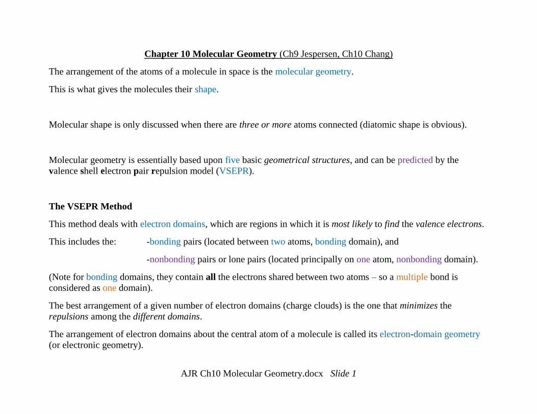
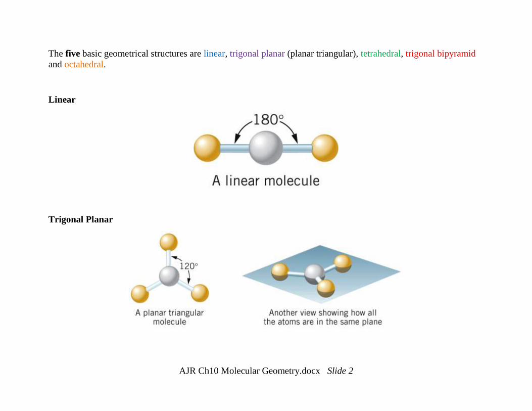
The five basic geometrical structures are linear, trigonal planar (planar triangular), tetrahedral, trigonal bipyramid
and octahedral.
Linear
Trigonal Planar
AJR Ch10 Molecular Geometry.docx Slide 3
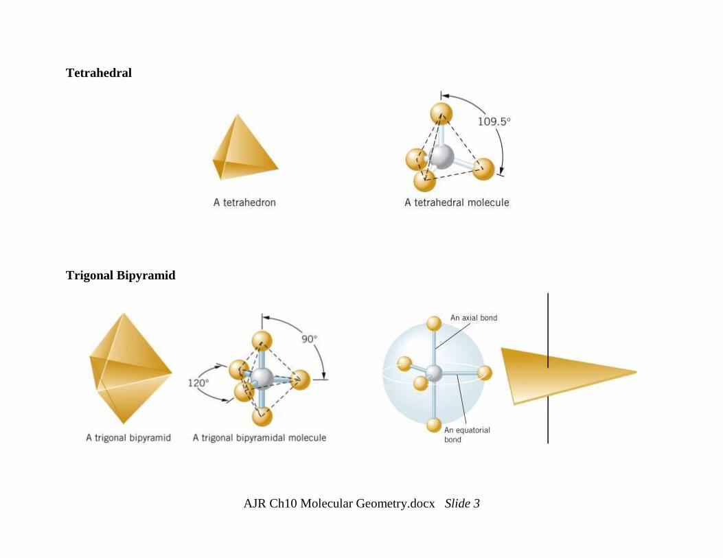
Tetrahedral
Trigonal Bipyramid
AJR Ch10 Molecular Geometry.docx Slide 4
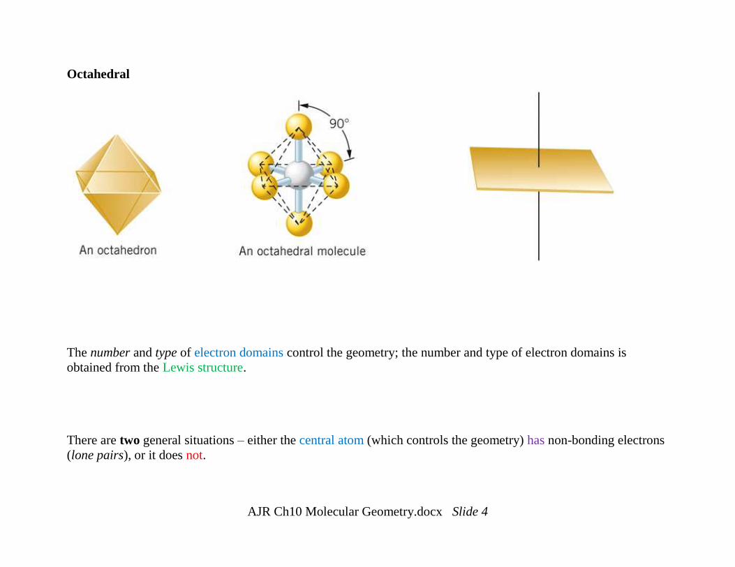
Octahedral
The number and type of electron domains control the geometry; the number and type of electron domains is
obtained from the Lewis structure.
There are two general situations – either the central atom (which controls the geometry) has non-bonding electrons
(lone pairs), or it does not.
AJR Ch10 Molecular Geometry.docx Slide 5
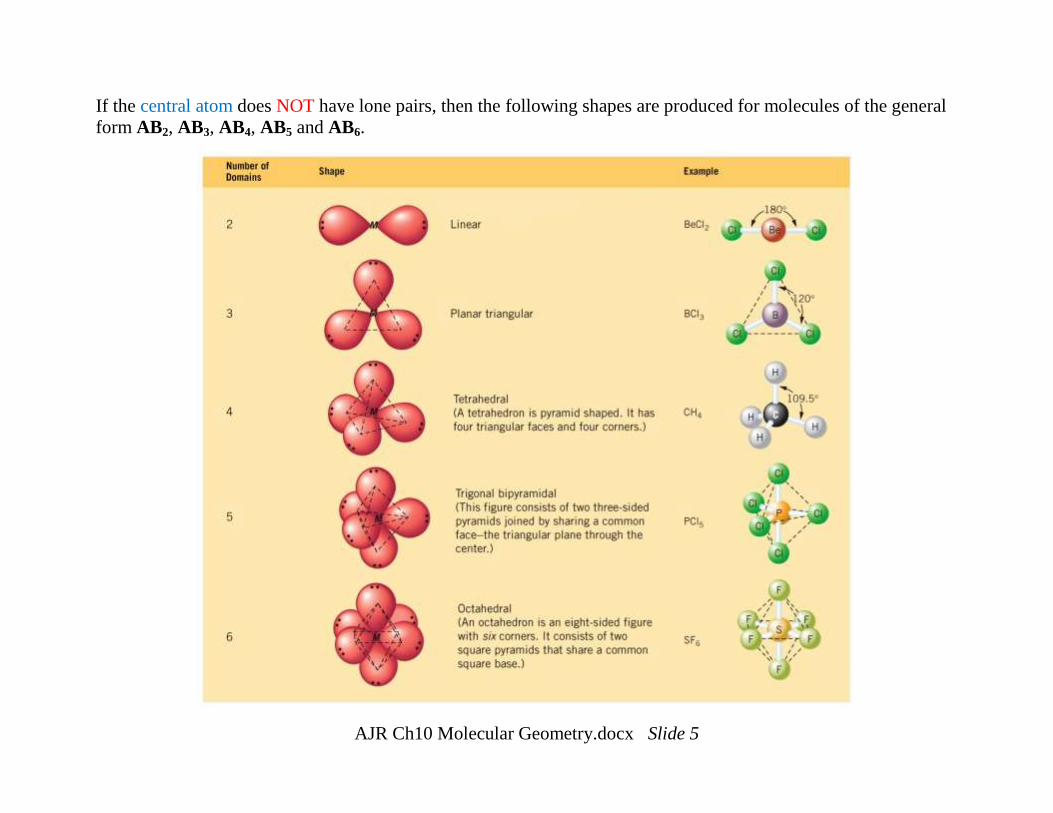
If the central atom does NOT have lone pairs, then the following shapes are produced for molecules of the general
form AB2, AB3, AB4, AB5 and AB6.
AJR Ch10 Molecular Geometry.docx Slide 6
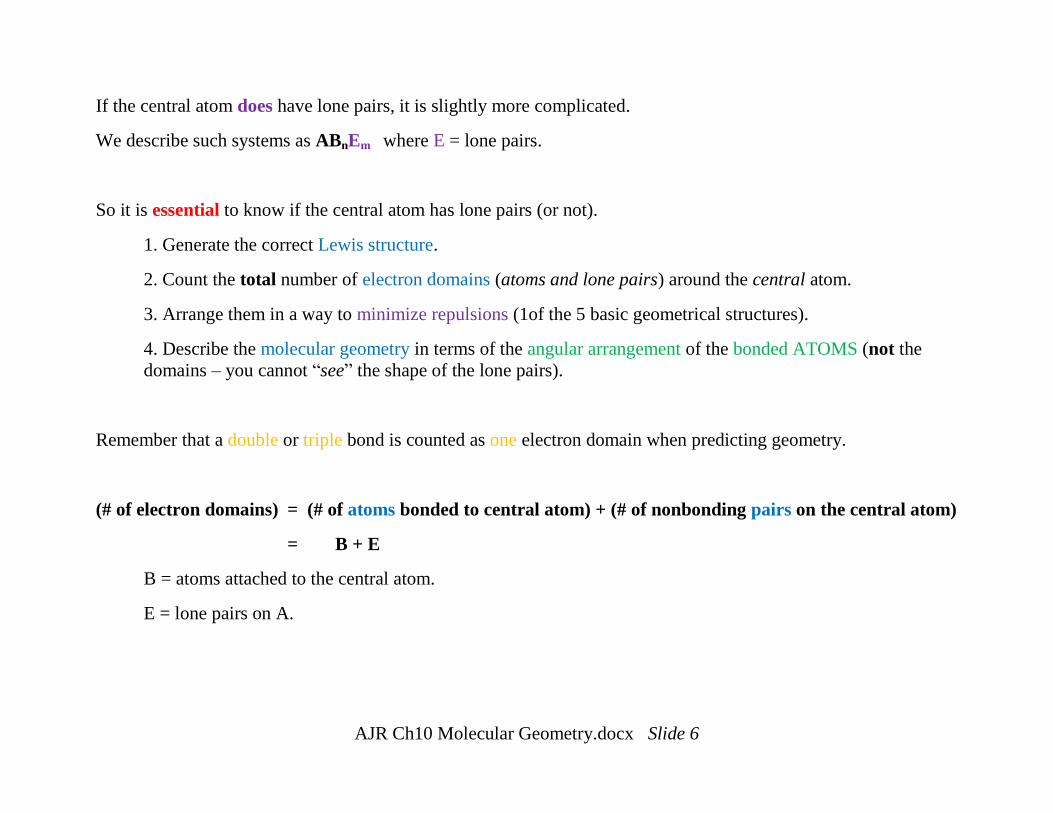
If the central atom does have lone pairs, it is slightly more complicated.
We describe such systems as ABnEm where E = lone pairs.
So it is essential to know if the central atom has lone pairs (or not).
1. Generate the correct Lewis structure.
2. Count the total number of electron domains (atoms and lone pairs) around the central atom.
3. Arrange them in a way to minimize repulsions (1of the 5 basic geometrical structures).
4. Describe the molecular geometry in terms of the angular arrangement of the bonded ATOMS (not the
domains – you cannot “see” the shape of the lone pairs).
Remember that a double or triple bond is counted as one electron domain when predicting geometry.
(# of electron domains) = (# of atoms bonded to central atom) + (# of nonbonding pairs on the central atom)
= B + E
B = atoms attached to the central atom.
E = lone pairs on A.
AJR Ch10 Molecular Geometry.docx Slide 7
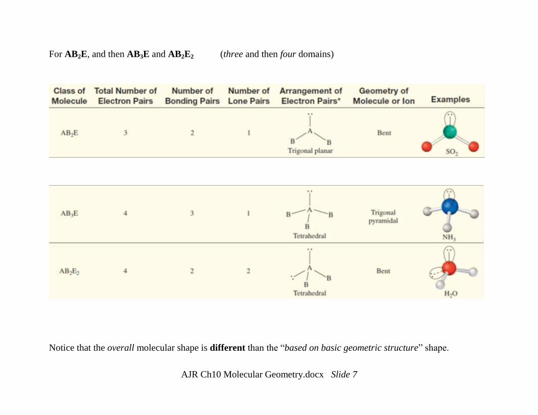
For AB2E, and then AB3E and AB2E2 (three and then four domains)
Notice that the overall molecular shape is different than the “based on basic geometric structure” shape.
AJR Ch10 Molecular Geometry.docx Slide 8
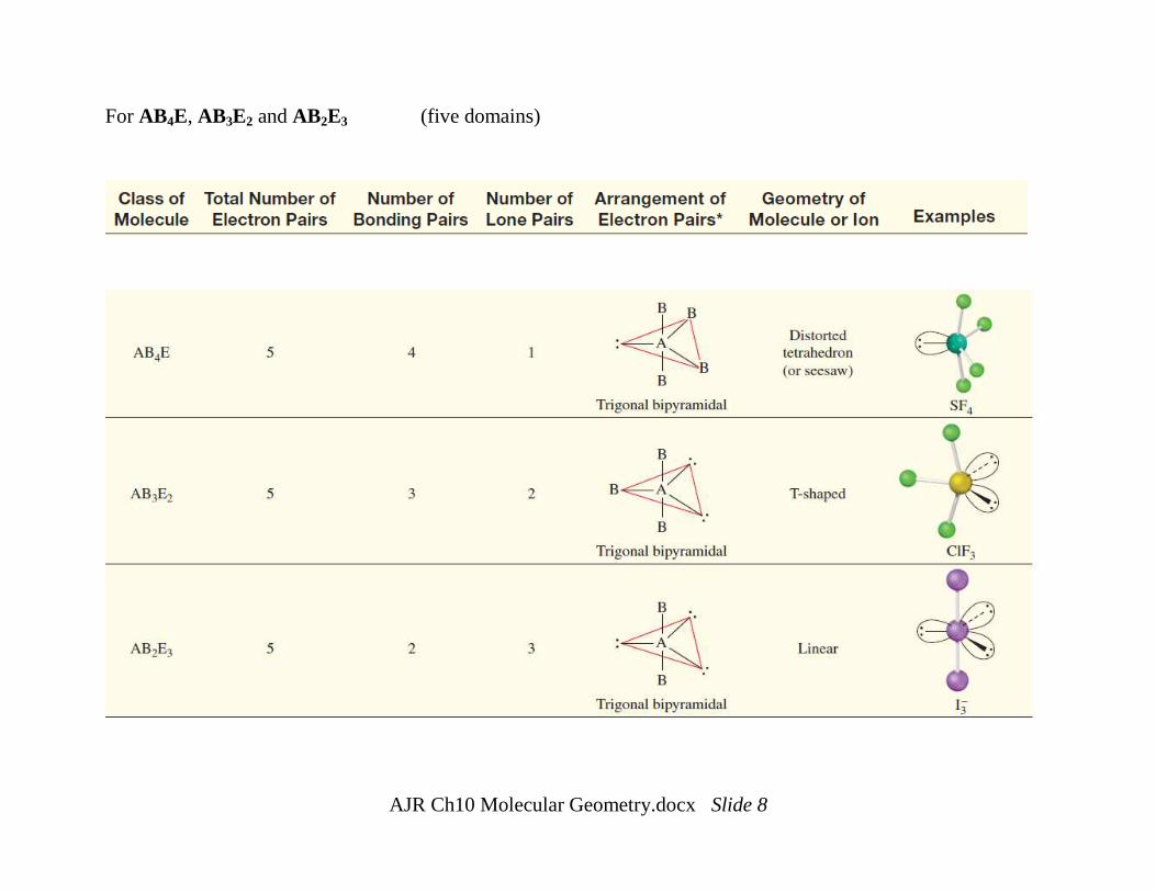
For AB4E, AB3E2 and AB2E3 (five domains)
AJR Ch10 Molecular Geometry.docx Slide 9
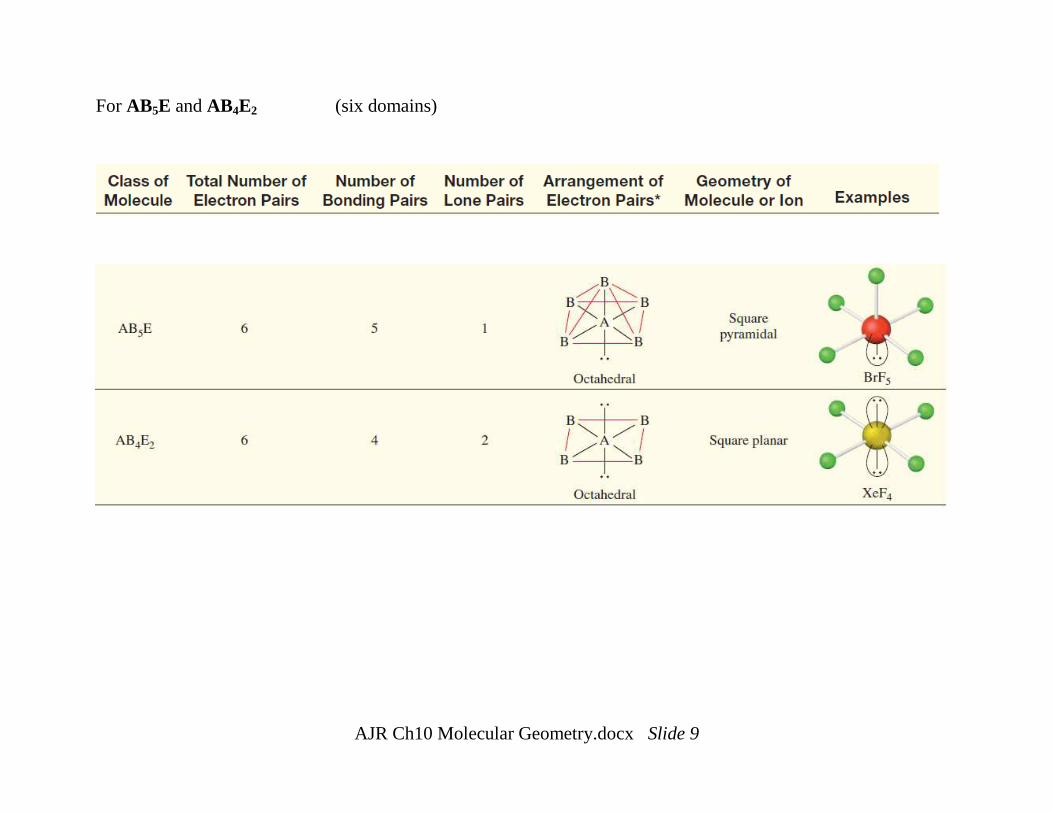
For AB5E and AB4E2 (six domains)
AJR Ch10 Molecular Geometry.docx Slide 10
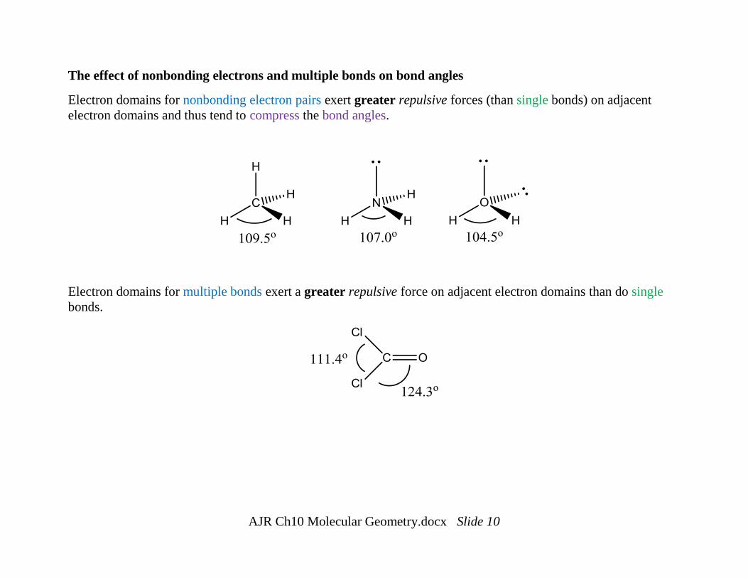
The effect of nonbonding electrons and multiple bonds on bond angles
Electron domains for nonbonding electron pairs exert greater repulsive forces (than single bonds) on adjacent
electron domains and thus tend to compress the bond angles.
Electron domains for multiple bonds exert a greater repulsive force on adjacent electron domains than do single
bonds.
AJR Ch10 Molecular Geometry.docx Slide 11
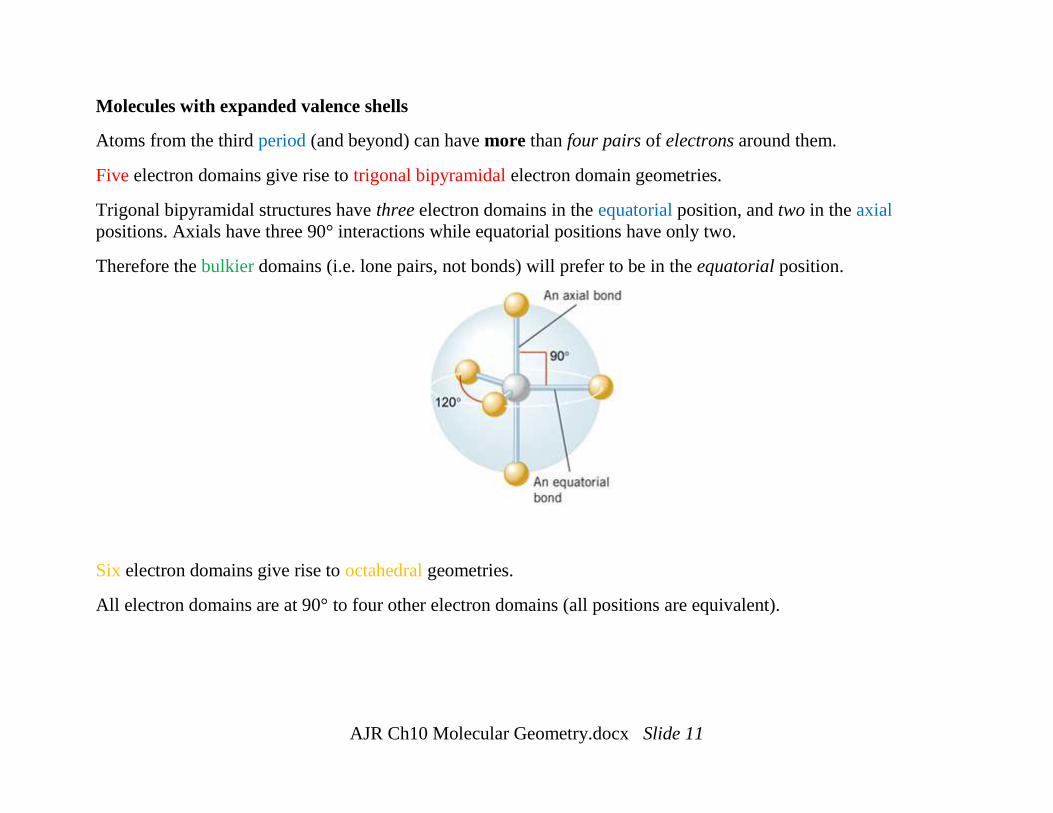
Molecules with expanded valence shells
Atoms from the third period (and beyond) can have more than four pairs of electrons around them.
Five electron domains give rise to trigonal bipyramidal electron domain geometries.
Trigonal bipyramidal structures have three electron domains in the equatorial position, and two in the axial
positions. Axials have three 90° interactions while equatorial positions have only two.
Therefore the bulkier domains (i.e. lone pairs, not bonds) will prefer to be in the equatorial position.
Six electron domains give rise to octahedral geometries.
All electron domains are at 90° to four other electron domains (all positions are equivalent).
AJR Ch10 Molecular Geometry.docx Slide 12
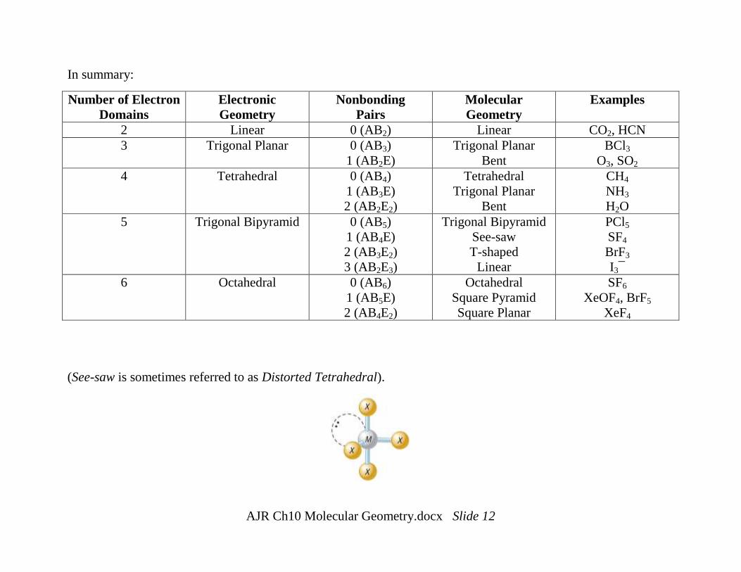
In summary:
Number of Electron
Domains
Electronic
Geometry
Nonbonding
Pairs
Molecular
Geometry
Examples
2 Linear 0 (AB2) Linear CO2, HCN
3 Trigonal Planar 0 (AB3)
1 (AB2E)
Trigonal Planar
Bent
BCl3
O3, SO2
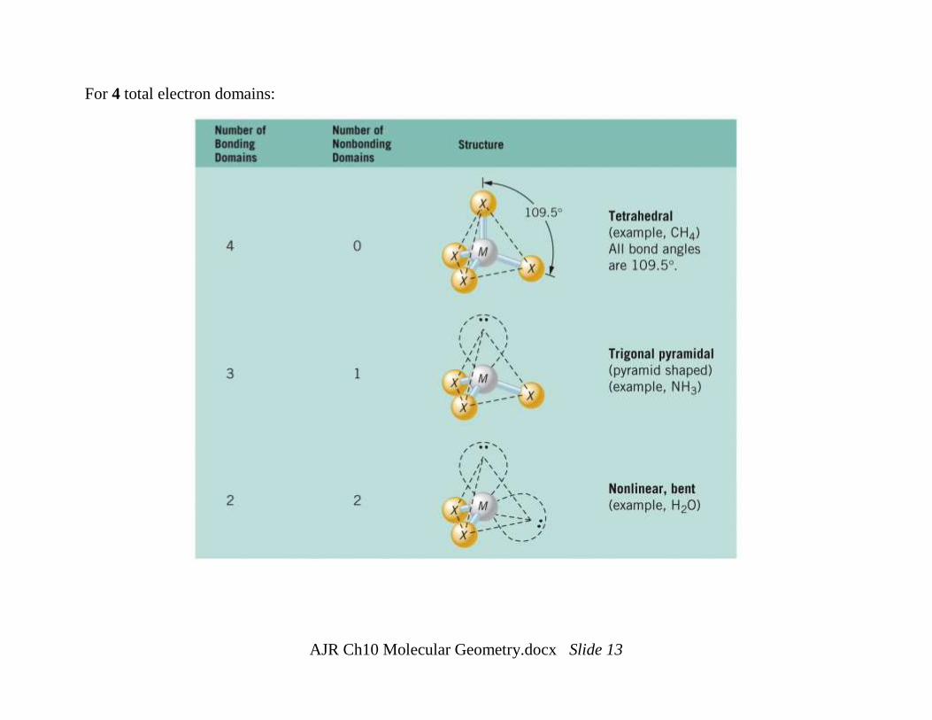
4 Tetrahedral 0 (AB4)
1 (AB3E)
2 (AB2E2)
Tetrahedral
Trigonal Planar
Bent
CH4
NH3
H2O
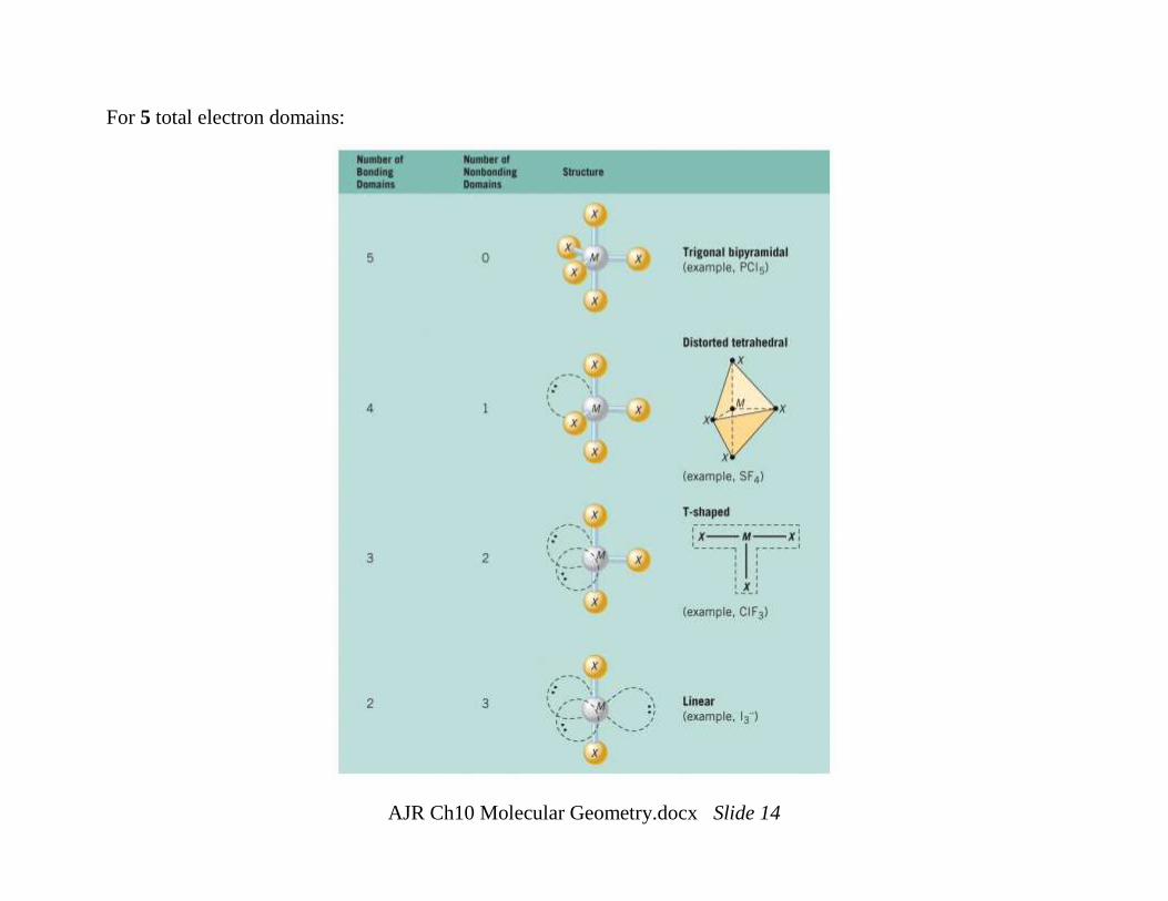
5 Trigonal Bipyramid 0 (AB5)
1 (AB4E)
2 (AB3E2)
3 (AB2E3)
Trigonal Bipyramid
See-saw
T-shaped
Linear
PCl5
SF4
BrF3
I3¯
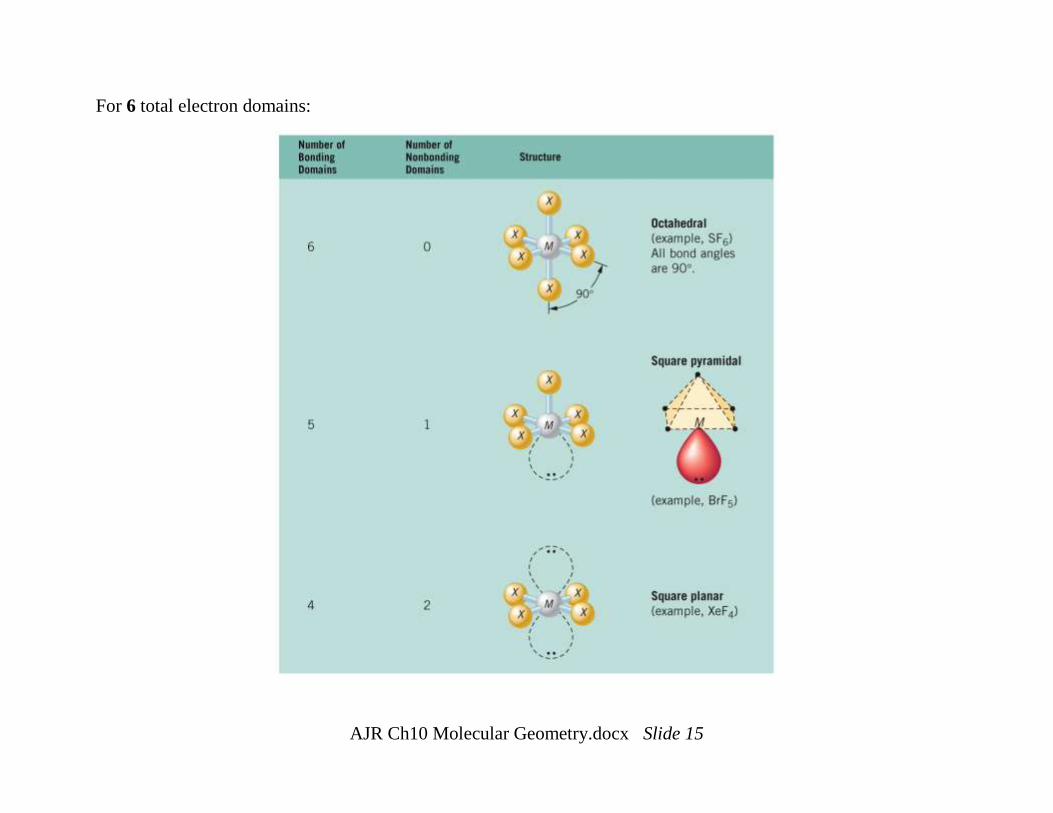
6 Octahedral 0 (AB6)
1 (AB5E)
2 (AB4E2)
Octahedral
Square Pyramid
Square Planar
SF6
XeOF4, BrF5
XeF4
(See-saw is sometimes referred to as Distorted Tetrahedral).
AJR Ch10 Molecular Geometry.docx Slide 13
For 4 total electron domains:
AJR Ch10 Molecular Geometry.docx Slide 14
For 5 total electron domains:
AJR Ch10 Molecular Geometry.docx Slide 15
For 6 total electron domains:
AJR Ch10 Molecular Geometry.docx Slide 16
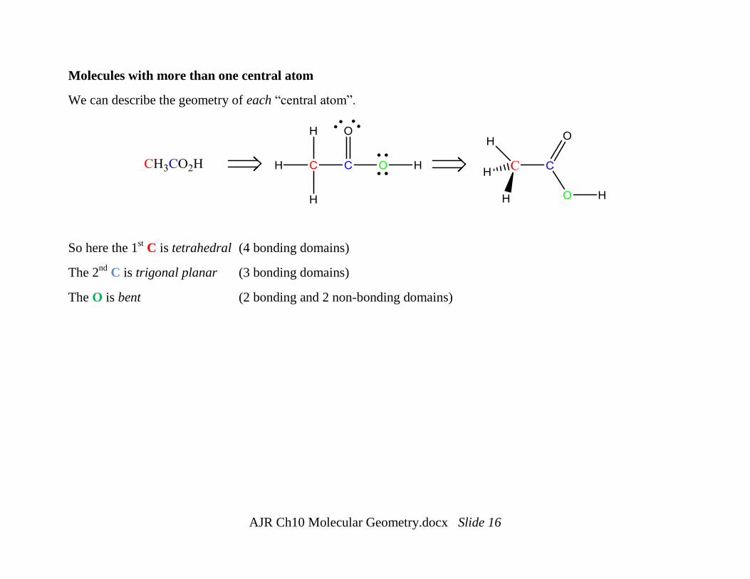
Molecules with more than one central atom
We can describe the geometry of each “central atom”.
So here the 1st C is tetrahedral (4 bonding domains)
The 2nd
C is trigonal planar (3 bonding domains)
The O is bent (2 bonding and 2 non-bonding domains)
AJR Ch10 Molecular Geometry.docx Slide 17
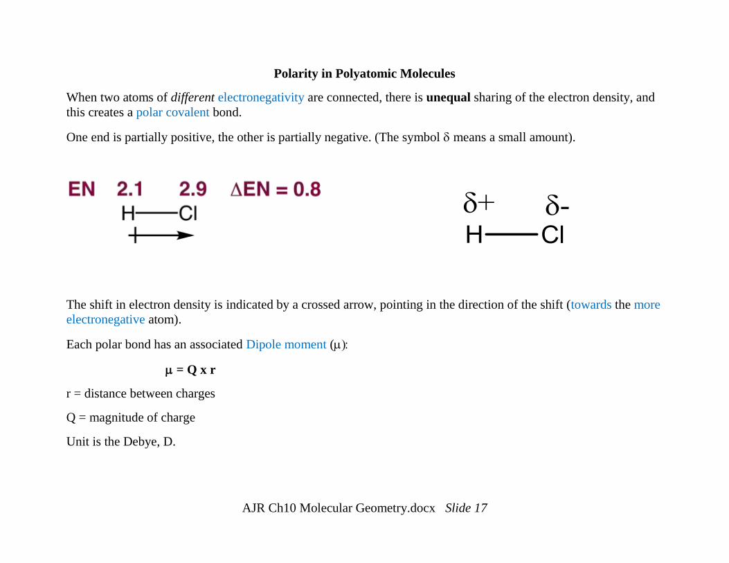
Polarity in Polyatomic Molecules
When two atoms of different electronegativity are connected, there is unequal sharing of the electron density, and
this creates a polar covalent bond.
One end is partially positive, the other is partially negative. (The symbol means a small amount).
The shift in electron density is indicated by a crossed arrow, pointing in the direction of the shift (towards the more
electronegative atom).
Each polar bond has an associated Dipole moment (
= Q x r
r = distance between charges
Q = magnitude of charge
Unit is the Debye, D.
AJR Ch10 Molecular Geometry.docx Slide 18
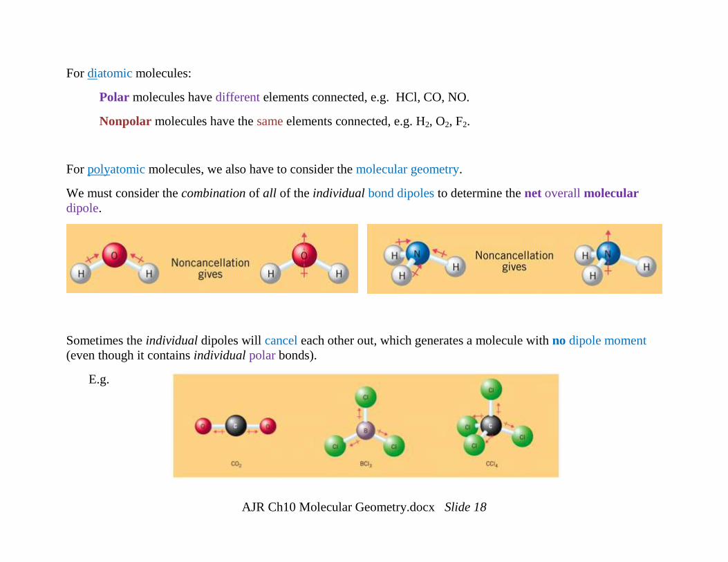
For diatomic molecules:
Polar molecules have different elements connected, e.g. HCl, CO, NO.
Nonpolar molecules have the same elements connected, e.g. H2, O2, F2.
For polyatomic molecules, we also have to consider the molecular geometry.
We must consider the combination of all of the individual bond dipoles to determine the net overall molecular
dipole.
Sometimes the individual dipoles will cancel each other out, which generates a molecule with no dipole moment
(even though it contains individual polar bonds).
E.g.
AJR Ch10 Molecular Geometry.docx Slide 19
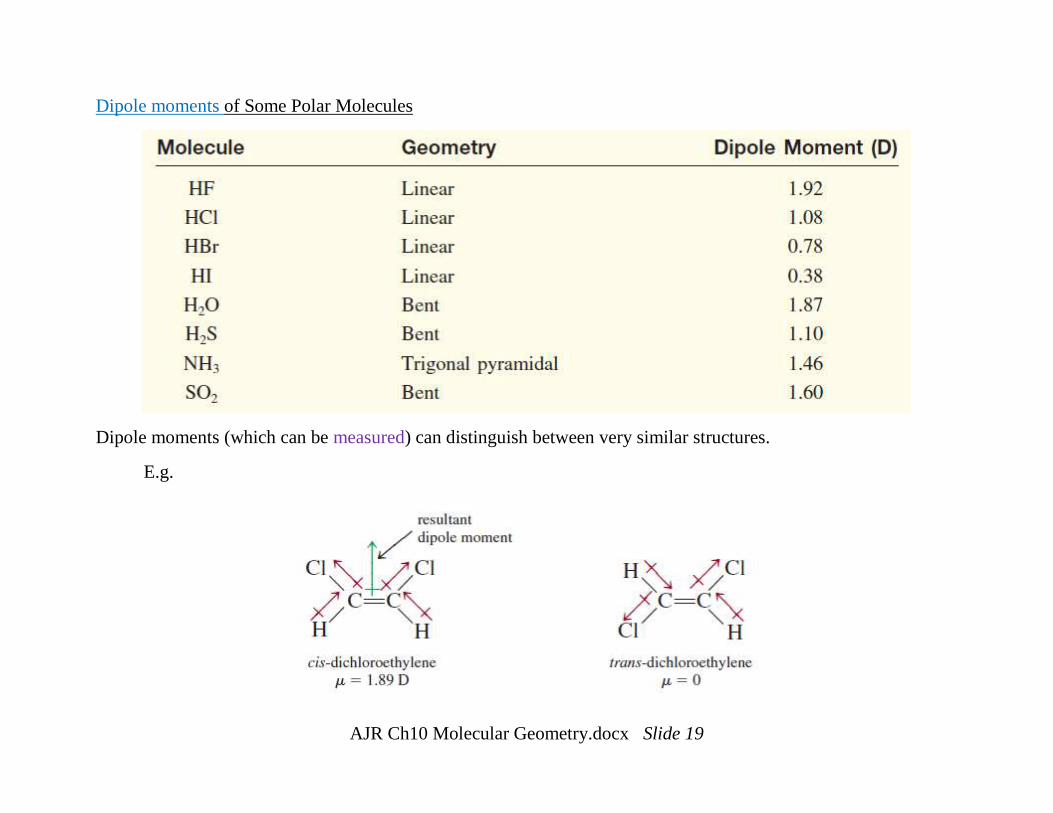
Dipole moments of Some Polar Molecules
Dipole moments (which can be measured) can distinguish between very similar structures.
E.g.
AJR Ch10 Molecular Geometry.docx Slide 20
Covalent Bonding
There are two different theories (approaches/perspectives) that are used to explain covalent bonding.
They are Valence Bond Theory (VB theory) and Molecular Orbital Theory (MO theory).
Essentially they are atomic and molecular perspectives of covalent bonding.
Valence-bond theory – the electrons in a molecule occupy atomic orbitals of the individual atoms.
In valence-bond theory, we assume that bonds form via the pairing of unpaired electrons in valence-shell atomic
orbitals.
The electrons can pair when their atomic orbitals overlap.
“Overlap” means that a portion of the atomic orbitals from each atom occupy the same region of space; or
Overlap = interaction/interference of wavefunctions.
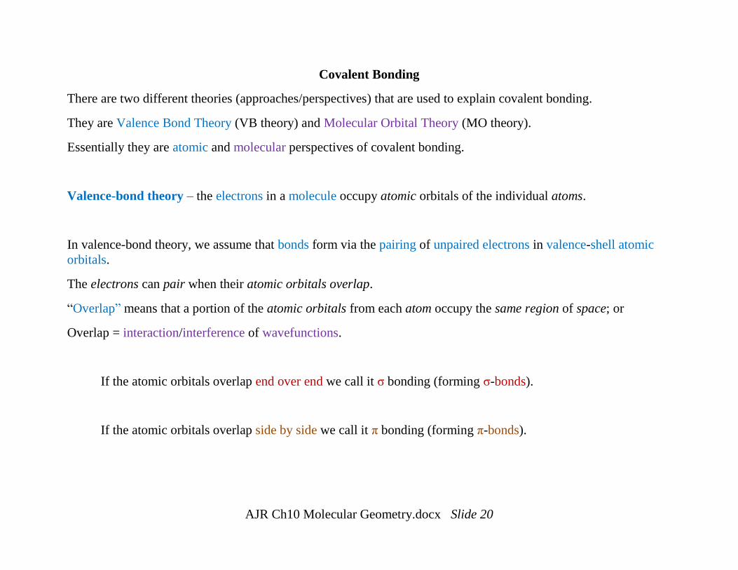
If the atomic orbitals overlap end over end we call it σ bonding (forming σ-bonds).
If the atomic orbitals overlap side by side we call it π bonding (forming π-bonds).
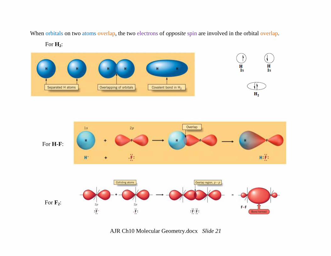
AJR Ch10 Molecular Geometry.docx Slide 21
When orbitals on two atoms overlap, the two electrons of opposite spin are involved in the orbital overlap.
For H2:
For H-F:
For F2:
AJR Ch10 Molecular Geometry.docx Slide 22
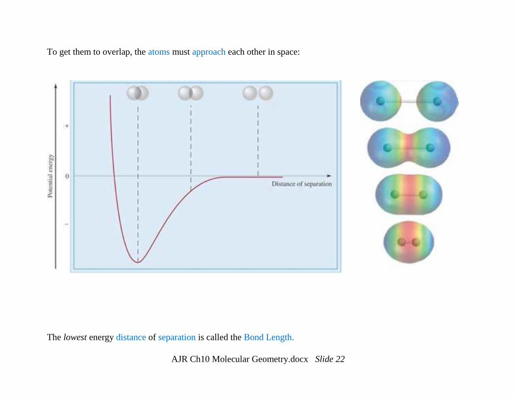
To get them to overlap, the atoms must approach each other in space:
The lowest energy distance of separation is called the Bond Length.
AJR Ch10 Molecular Geometry.docx Slide 23
Lewis theory basically says two electrons make a covalent bond; VB theory says which two electrons (and in doing
so explains different bond strengths/energies) – but it still does not explain tetrahedral geometries.
This prompted the idea of Hybrid Atomic Orbitals. (Hybrid = mixture).
Hybrid atomic orbitals are the mathematical combination of wavefunctions on the same atom to form a new set
of equivalent wavefunctions called hybrid atomic wavefunctions.
The mixing of n atomic orbitals always results in n hybrid orbitals.
AJR Ch10 Molecular Geometry.docx Slide 24
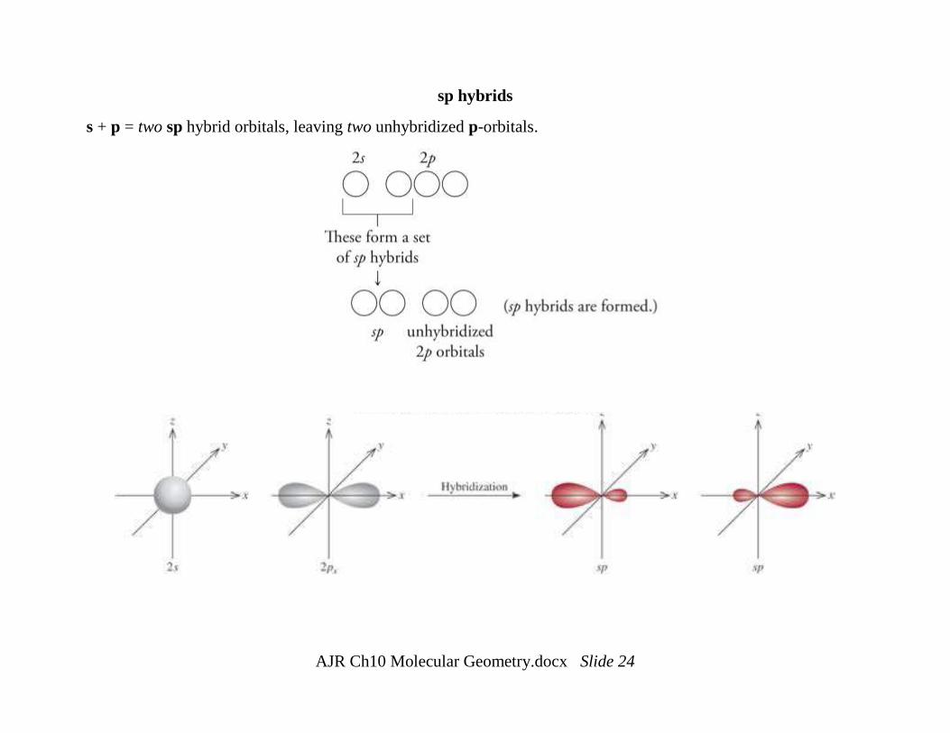
sp hybrids
s + p = two sp hybrid orbitals, leaving two unhybridized p-orbitals.
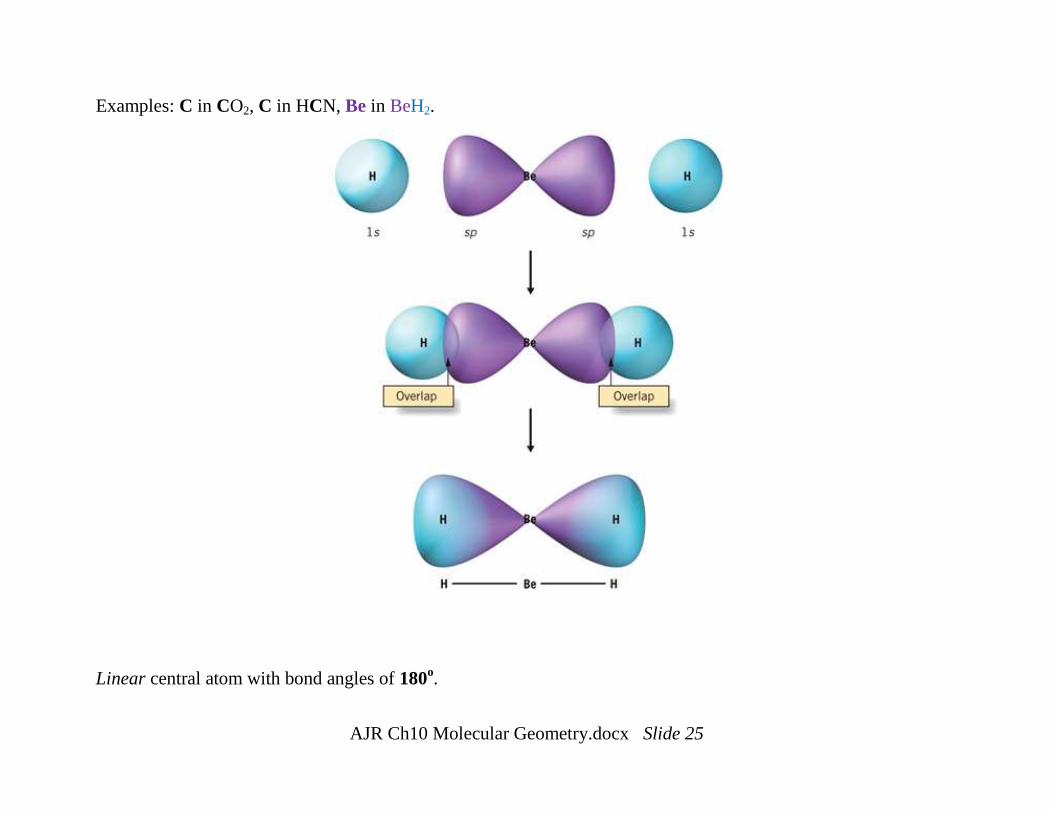
AJR Ch10 Molecular Geometry.docx Slide 25
Examples: C in CO2, C in HCN, Be in BeH2.
Linear central atom with bond angles of 180o.
AJR Ch10 Molecular Geometry.docx Slide 26
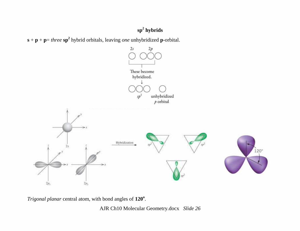
sp2 hybrids
s + p + p= three sp2 hybrid orbitals, leaving one unhybridized p-orbital.
Trigonal planar central atom, with bond angles of 120o.
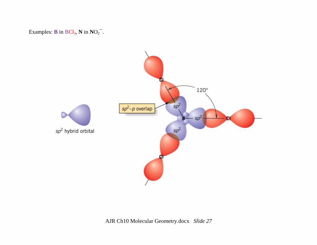
AJR Ch10 Molecular Geometry.docx Slide 27
Examples: B in BCl3, N in NO2¯.
AJR Ch10 Molecular Geometry.docx Slide 28
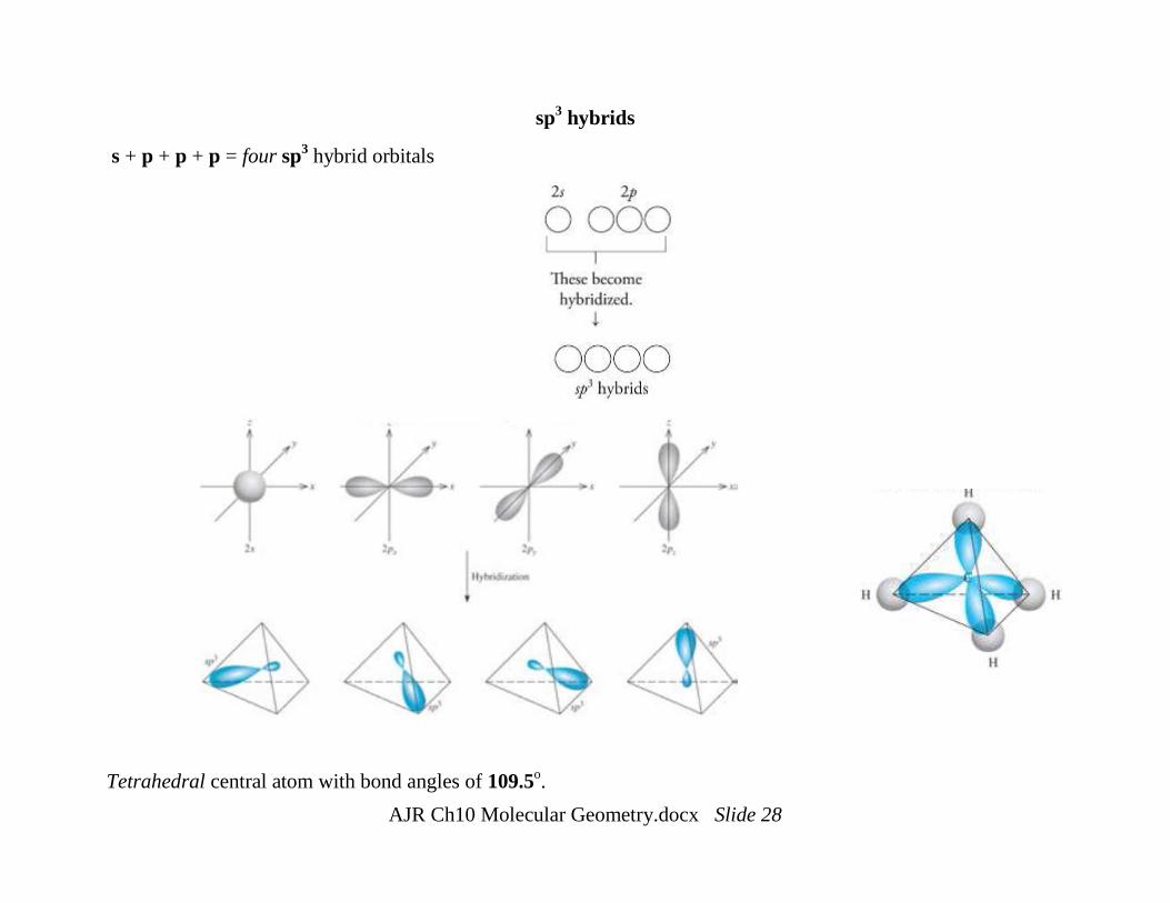
sp3 hybrids
s + p + p + p = four sp3 hybrid orbitals
Tetrahedral central atom with bond angles of 109.5o.
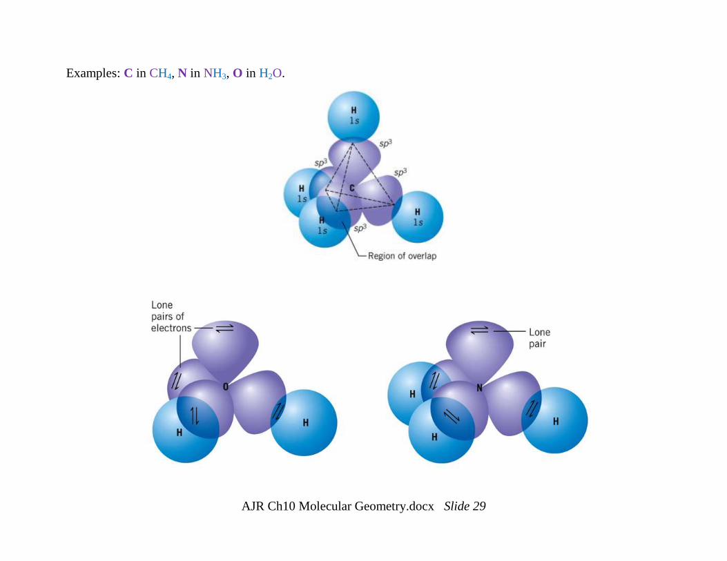
AJR Ch10 Molecular Geometry.docx Slide 29
Examples: C in CH4, N in NH3, O in H2O.
AJR Ch10 Molecular Geometry.docx Slide 30
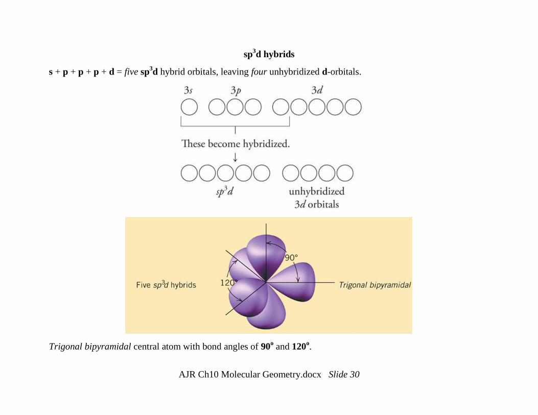
sp3d hybrids
s + p + p + p + d = five sp3d hybrid orbitals, leaving four unhybridized d-orbitals.
Trigonal bipyramidal central atom with bond angles of 90o and 120
o.
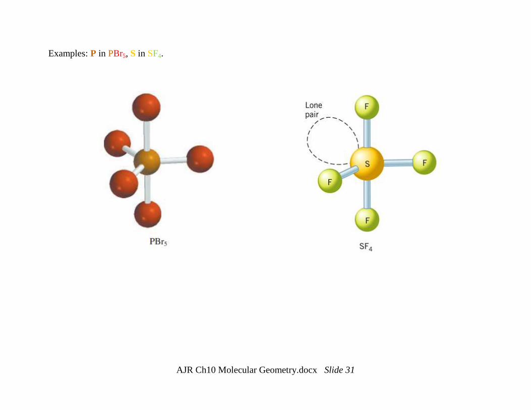
AJR Ch10 Molecular Geometry.docx Slide 31
Examples: P in PBr5, S in SF4.
AJR Ch10 Molecular Geometry.docx Slide 32
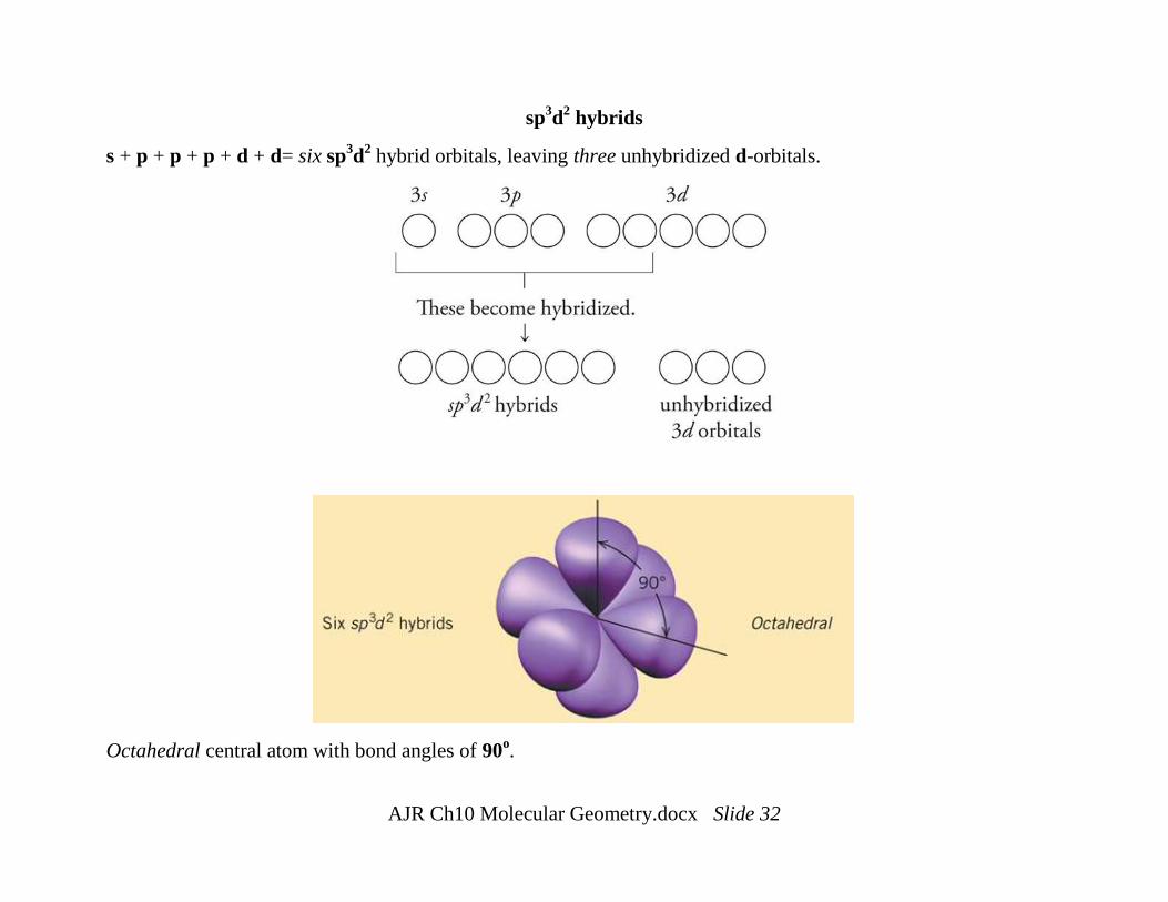
sp3d
2 hybrids
s + p + p + p + d + d= six sp3d
2 hybrid orbitals, leaving three unhybridized d-orbitals.
Octahedral central atom with bond angles of 90o.
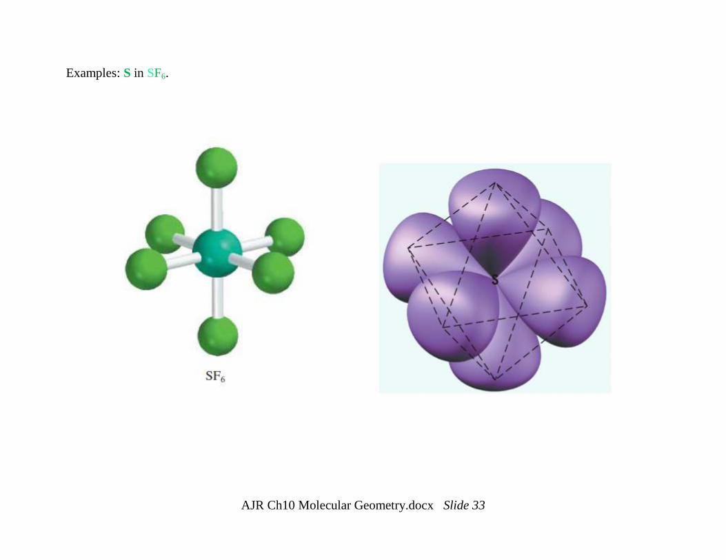
AJR Ch10 Molecular Geometry.docx Slide 33
Examples: S in SF6.
AJR Ch10 Molecular Geometry.docx Slide 34
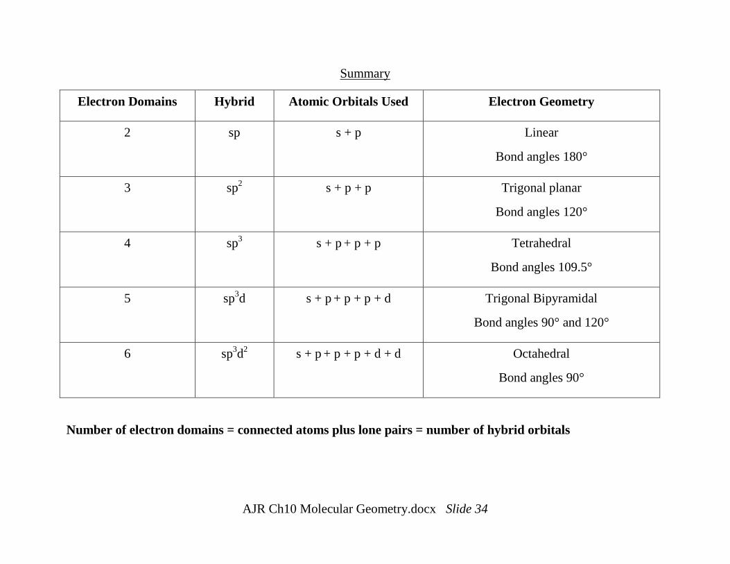
Summary
Electron Domains Hybrid Atomic Orbitals Used Electron Geometry
2 sp s + p Linear
Bond angles 180°
3 sp2 s + p + p Trigonal planar
Bond angles 120°
4 sp3 s + p + p + p Tetrahedral
Bond angles 109.5°
5 sp3d s + p + p + p + d Trigonal Bipyramidal
Bond angles 90° and 120°
6 sp3d
2 s + p + p + p + d + d Octahedral
Bond angles 90°
Number of electron domains = connected atoms plus lone pairs = number of hybrid orbitals
AJR Ch10 Molecular Geometry.docx Slide 35
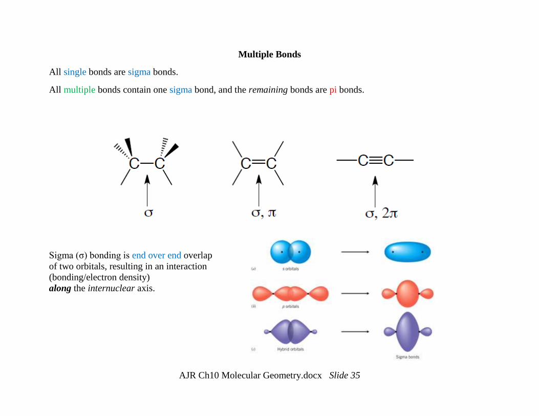
Multiple Bonds
All single bonds are sigma bonds.
All multiple bonds contain one sigma bond, and the remaining bonds are pi bonds.
Sigma (σ) bonding is end over end overlap
of two orbitals, resulting in an interaction
(bonding/electron density)
along the internuclear axis.
AJR Ch10 Molecular Geometry.docx Slide 36
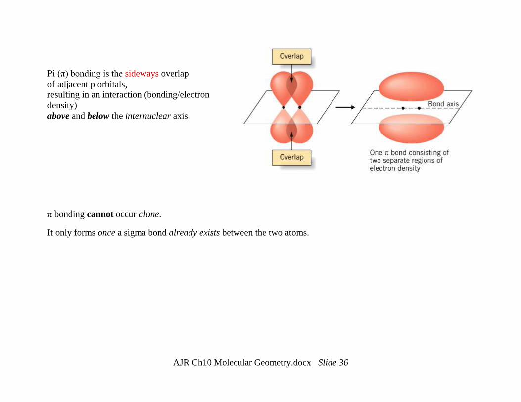
Pi (π) bonding is the sideways overlap
of adjacent p orbitals,
resulting in an interaction (bonding/electron
density)
above and below the internuclear axis.
π bonding cannot occur alone.
It only forms once a sigma bond already exists between the two atoms.
AJR Ch10 Molecular Geometry.docx Slide 37
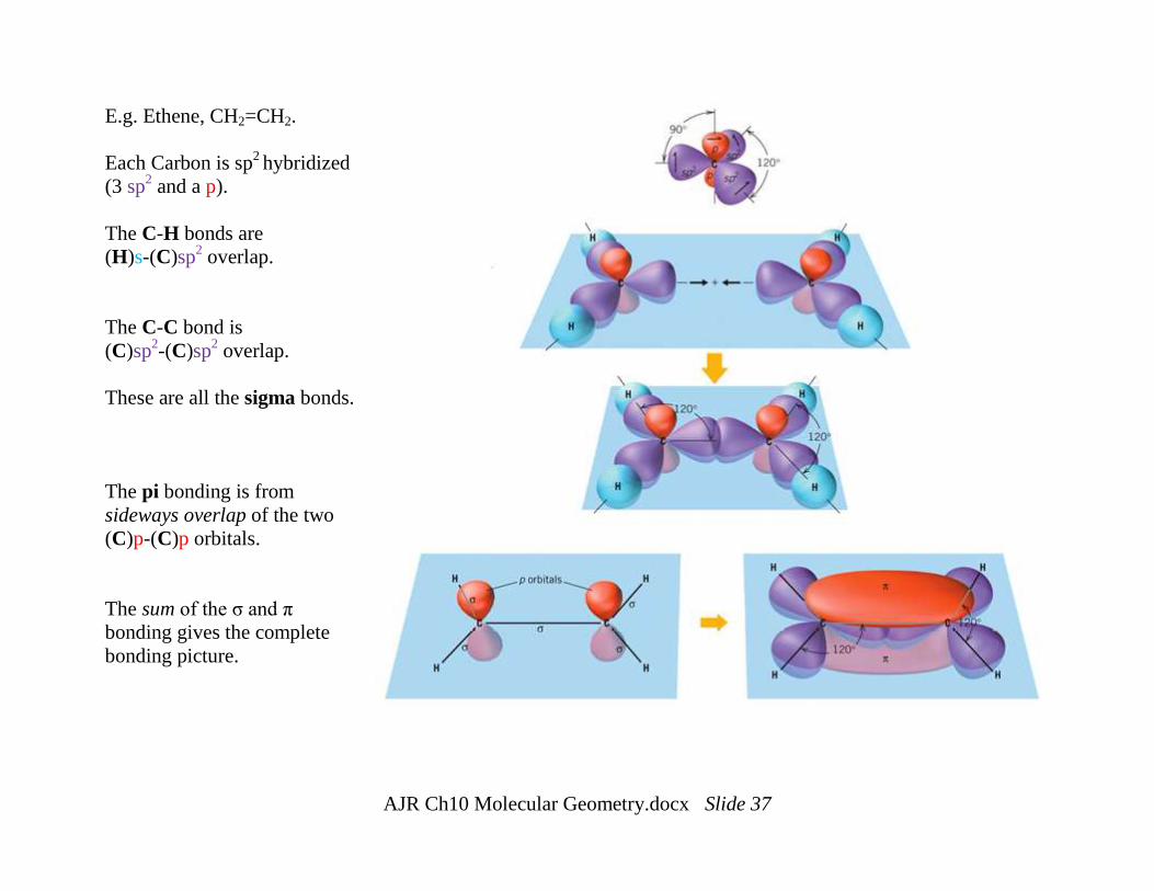
E.g. Ethene, CH2=CH2.
Each Carbon is sp2
hybridized
(3 sp2 and a p).
The C-H bonds are
(H)s-(C)sp2 overlap.
The C-C bond is
(C)sp2-(C)sp
2 overlap.
These are all the sigma bonds.
The pi bonding is from
sideways overlap of the two
(C)p-(C)p orbitals.
The sum of the σ and π
bonding gives the complete
bonding picture.
AJR Ch10 Molecular Geometry.docx Slide 38
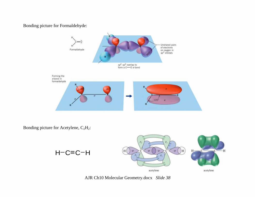
Bonding picture for Formaldehyde:
Bonding picture for Acetylene, C2H2:
C C HH
AJR Ch10 Molecular Geometry.docx Slide 39
Molecular Orbital (MO) Theory
There is also an alternative to VB Theory to describe bonding in molecules – Molecular Orbital Theory.
A molecular orbital is a mathematical function that describes the wave-like behavior of an electron in a molecule.
The molecular orbital is associated with the entire molecule.
Molecular orbitals form from the overlap of atomic orbitals.
Overlap of n atomic orbitals results in n molecular orbitals.
Sigma interaction of two AO’s generates two MO’s, one is bonding and one is anti-bonding.
We call these the σ and σ* molecular orbitals.
To discuss these interactions we need to recall:
Electrons are waves.
Waves have associated wavefunctions, ψ.
When overlapping/interacting waves, they interfere with each other.
Depending on the wavefunctions, this can be constructive or destructive.
AJR Ch10 Molecular Geometry.docx Slide 40
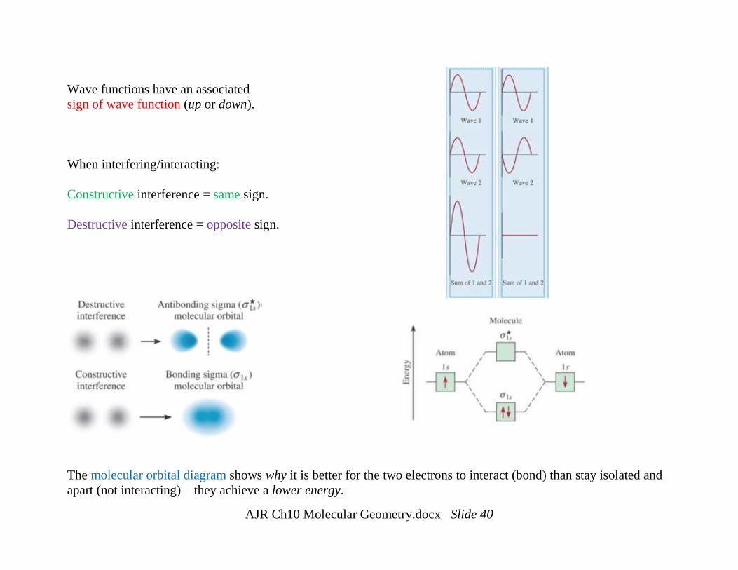
Wave functions have an associated
sign of wave function (up or down).
When interfering/interacting:
Constructive interference = same sign.
Destructive interference = opposite sign.
The molecular orbital diagram shows why it is better for the two electrons to interact (bond) than stay isolated and
apart (not interacting) – they achieve a lower energy.
AJR Ch10 Molecular Geometry.docx Slide 41
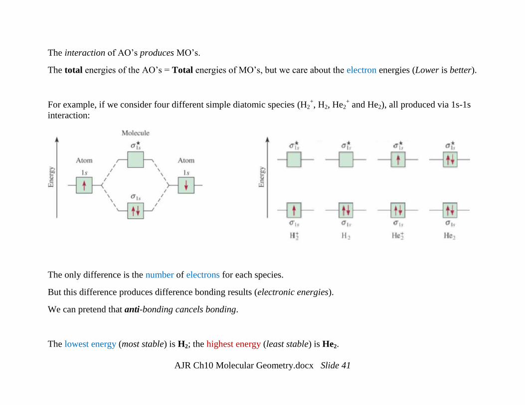
The interaction of AO’s produces MO’s.
The total energies of the AO’s = Total energies of MO’s, but we care about the electron energies (Lower is better).
For example, if we consider four different simple diatomic species (H2+, H2, He2
+ and He2), all produced via 1s-1s
interaction:
The only difference is the number of electrons for each species.
But this difference produces difference bonding results (electronic energies).
We can pretend that anti-bonding cancels bonding.
The lowest energy (most stable) is H2; the highest energy (least stable) is He2.
AJR Ch10 Molecular Geometry.docx Slide 42
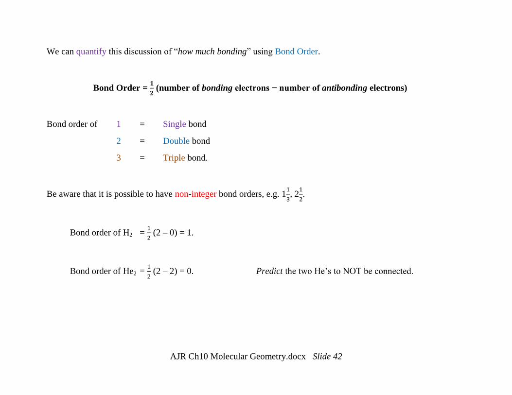
We can quantify this discussion of “how much bonding” using Bond Order.
Bond Order = 𝟏
𝟐 (number of bonding electrons − number of antibonding electrons)
Bond order of 1 = Single bond
2 = Double bond
3 = Triple bond.
Be aware that it is possible to have non-integer bond orders, e.g. 11
3, 2
1
2.
Bond order of H2 = 1
2 (2 – 0) = 1.
Bond order of He2 = 1
2 (2 – 2) = 0. Predict the two He’s to NOT be connected.
AJR Ch10 Molecular Geometry.docx Slide 43
Second-Row Diatomic Molecules
We can extend our MO theory to more larger, more complicated molecules.
If we look at the second row elements, and consider homonuclear diatomics – these will be bonding/interacting
using the 2s and three 2p orbitals.
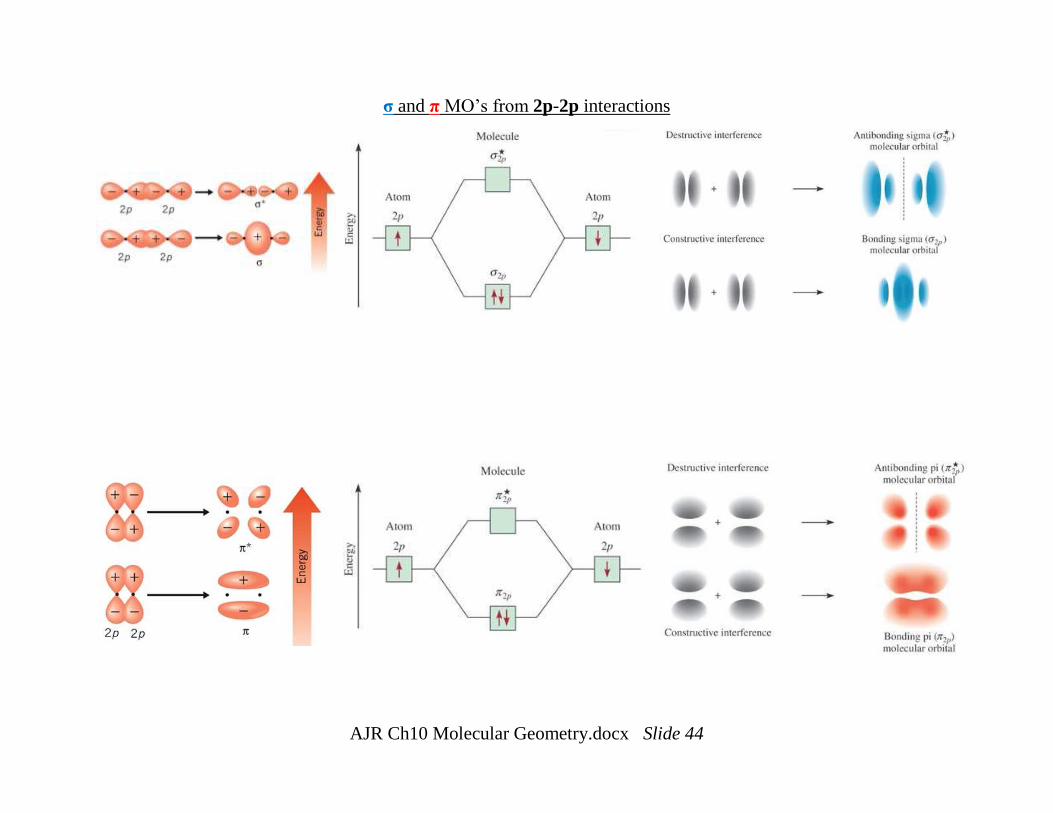
Atomic orbitals interact most effectively with other atomic orbitals of similar energy and shape.
So we see 1s interact with 1s, 2s interact with 2s, 2p interact with 2p, etc.
We already talked about how p orbitals can interact in either or both σ and π fashion, and this can lead to sigma (σ
and σ*) MO’s, and pi (π and π*) MO’s.
AJR Ch10 Molecular Geometry.docx Slide 44
σ and π MO’s from 2p-2p interactions
AJR Ch10 Molecular Geometry.docx Slide 45
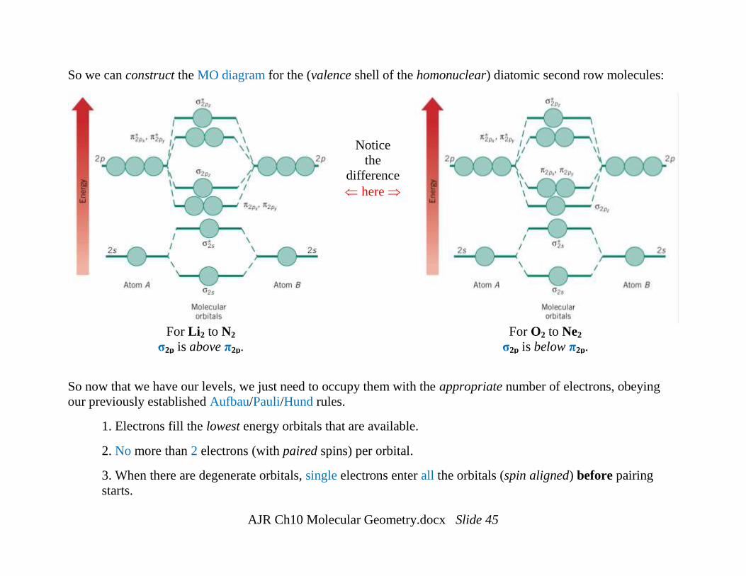
So we can construct the MO diagram for the (valence shell of the homonuclear) diatomic second row molecules:
Notice
the
difference
here
For Li2 to N2
σ2p is above π2p.
For O2 to Ne2
σ2p is below π2p.
So now that we have our levels, we just need to occupy them with the appropriate number of electrons, obeying
our previously established Aufbau/Pauli/Hund rules.
1. Electrons fill the lowest energy orbitals that are available.
2. No more than 2 electrons (with paired spins) per orbital.
3. When there are degenerate orbitals, single electrons enter all the orbitals (spin aligned) before pairing
starts.
AJR Ch10 Molecular Geometry.docx Slide 46
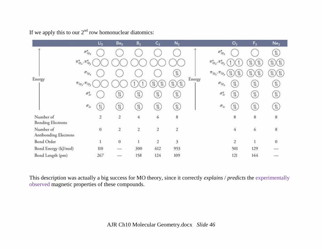
If we apply this to our 2nd
row homonuclear diatomics:
This description was actually a big success for MO theory, since it correctly explains / predicts the experimentally
observed magnetic properties of these compounds.
AJR Ch10 Molecular Geometry.docx Slide 47
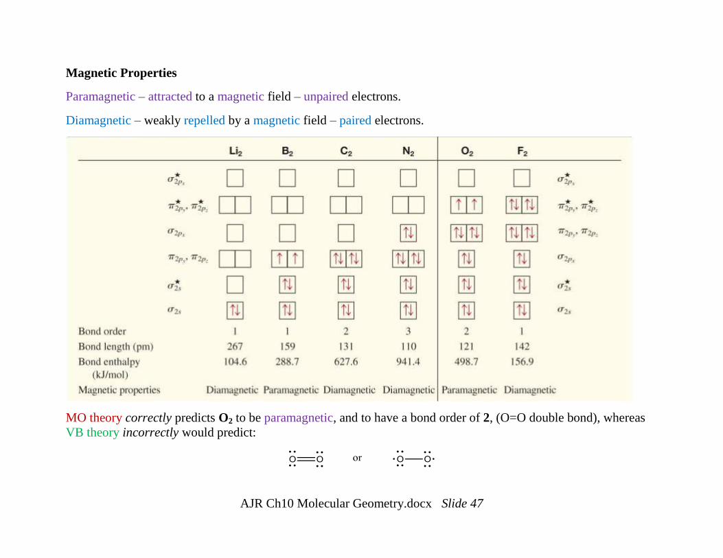
Magnetic Properties
Paramagnetic – attracted to a magnetic field – unpaired electrons.
Diamagnetic – weakly repelled by a magnetic field – paired electrons.
MO theory correctly predicts O2 to be paramagnetic, and to have a bond order of 2, (O=O double bond), whereas
VB theory incorrectly would predict: