Embed Size (px)
Citation preview
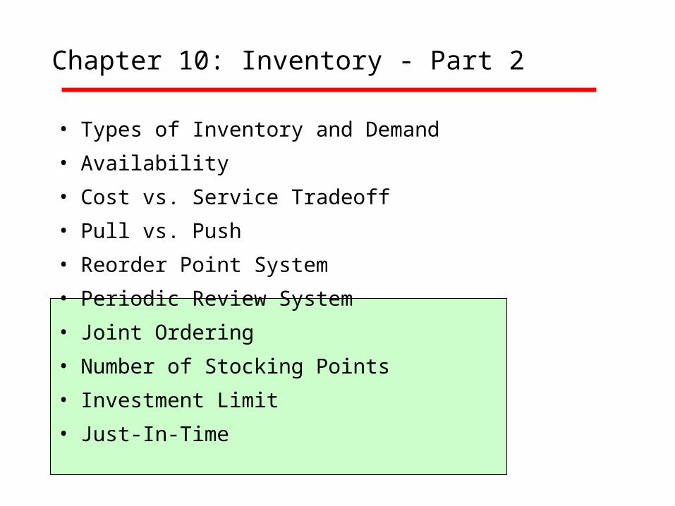
Chapter 10: Inventory - Part 2
• Types of Inventory and Demand
• Availability
• Cost vs. Service Tradeoff
• Pull vs. Push
• Reorder Point System
• Periodic Review System
• Joint Ordering
• Number of Stocking Points
• Investment Limit
• Just-In-Time
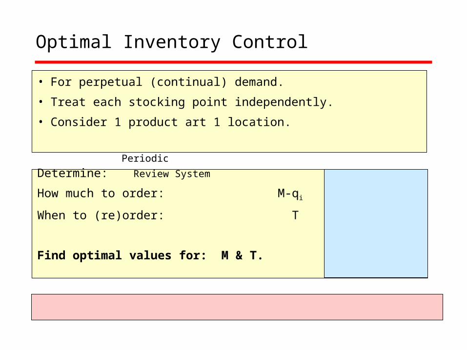
Optimal Inventory Control
• For perpetual (continual) demand.
• Treat each stocking point independently.
• Consider 1 product art 1 location.
Periodic
Determine: Review System
How much to order: M-qi
When to (re)order: T
Find optimal values for: M & T.
0
10
20
30
40
50
60
70
80
90
100
0 10 20 30 40 50 60 70 80 90
Time (days)
INV
EN
TO
RY
Inventory Level
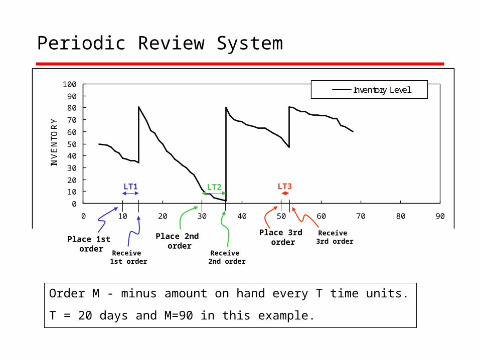
Periodic Review System
Receive 1st order
Place 1st order
Receive 2nd order
Place 2nd order
Receive 3rd order
Place 3rd order
LT1 LT2 LT3
Order M - minus amount on hand every T time units.
T = 20 days and M=90 in this example.
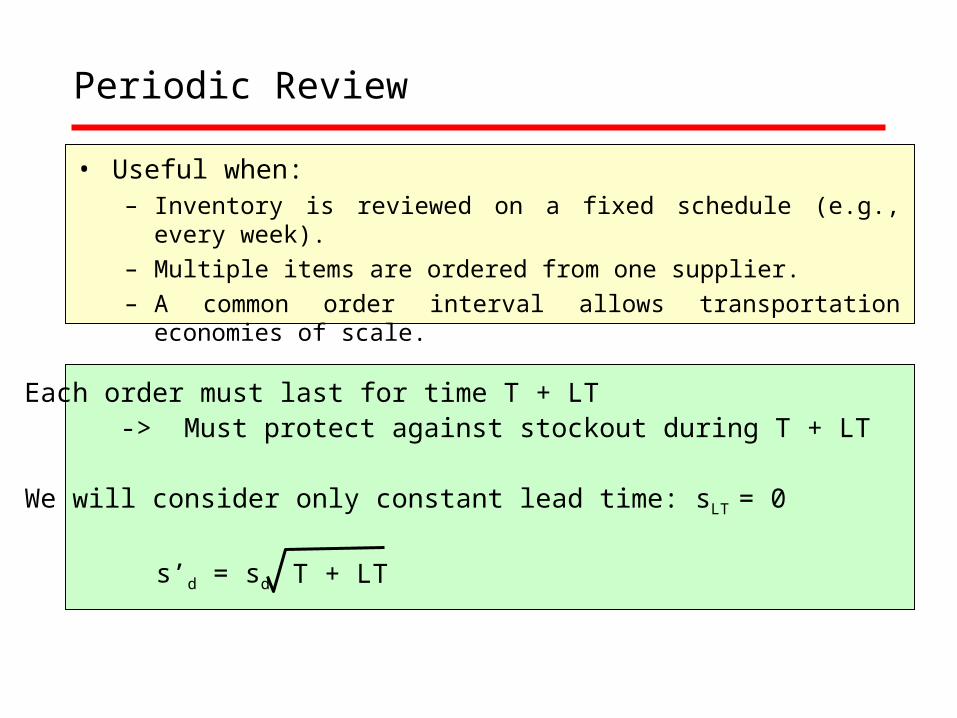
Periodic Review
• Useful when:– Inventory is reviewed on a fixed schedule (e.g., every week).– Multiple items are ordered from one supplier.– A common order interval allows transportation economies of
scale.
Each order must last for time T + LT-> Must protect against stockout during T + LT
We will consider only constant lead time: sLT = 0
T + LTs’d = sd
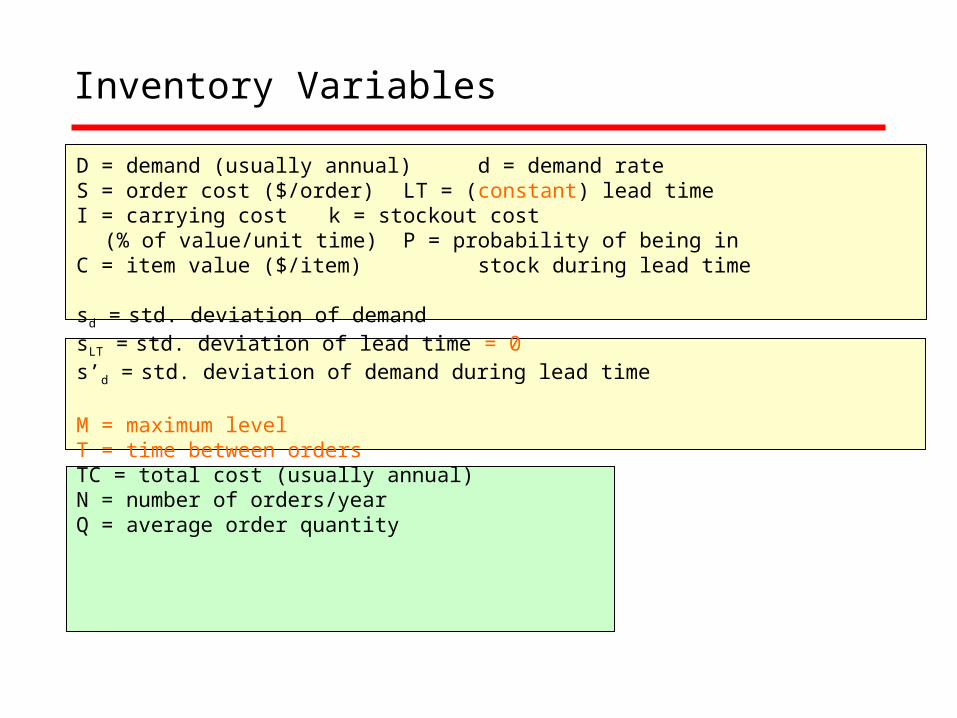
D = demand (usually annual) d = demand rateS = order cost ($/order) LT = (constant) lead timeI = carrying cost k = stockout cost
(% of value/unit time) P = probability of being inC = item value ($/item) stock during lead time
sd = std. deviation of demandsLT = std. deviation of lead time = 0s’d = std. deviation of demand during lead time
M = maximum levelT = time between ordersTC = total cost (usually annual) N = number of orders/yearQ = average order quantity
Inventory Variables
Periodic Review - Optimal Ordering
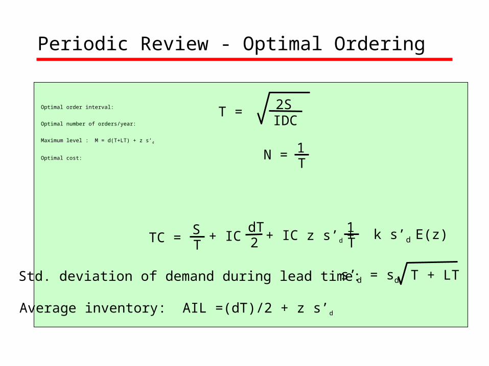
Optimal order interval:
Optimal number of orders/year:
Maximum level : M = d(T+LT) + z s’d
Optimal cost:
2ST =IDC
T1N =
TC = TS + IC 2
dT+ IC z s’d + T
1 k s’d E(z)
T + LTs’d = sdStd. deviation of demand during lead time:
Average inventory: AIL =(dT)/2 + z s’d
3 Cases
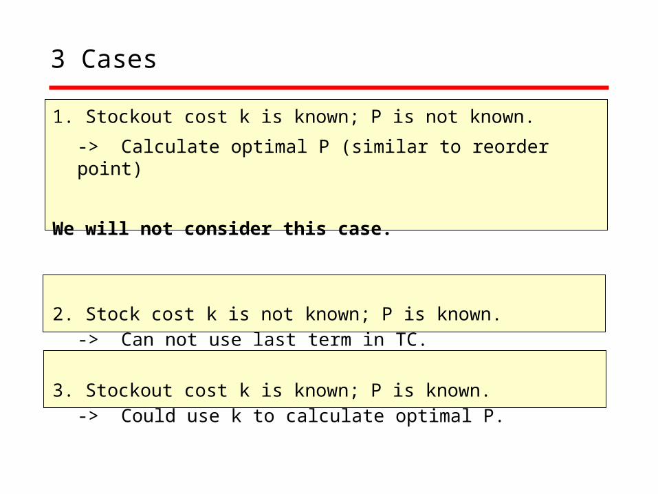
1. Stockout cost k is known; P is not known.
-> Calculate optimal P (similar to reorder point)
We will not consider this case.
2. Stock cost k is not known; P is known.-> Can not use last term in TC.
3. Stockout cost k is known; P is known.-> Could use k to calculate optimal P.
Periodic Review Example (same as Reorder Point)
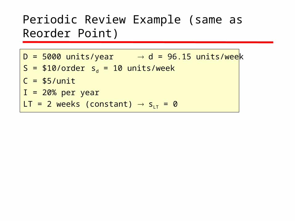
D = 5000 units/year d = 96.15 units/weekS = $10/order sd = 10 units/week
C = $5/unitI = 20% per yearLT = 2 weeks (constant) sLT = 0
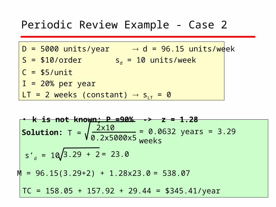
Periodic Review Example - Case 2
D = 5000 units/year d = 96.15 units/weekS = $10/order sd = 10 units/week
C = $5/unitI = 20% per yearLT = 2 weeks (constant) sLT = 0
• k is not known; P =90% -> z = 1.28
T =2x10
0.2x5000x5= 0.0632 years = 3.29 weeksSolution:
TC = 158.05 + 157.92 + 29.44 = $345.41/year
M = 96.15(3.29+2) + 1.28x23.0 = 538.07
3.29 + 2s’d = 10 = 23.0
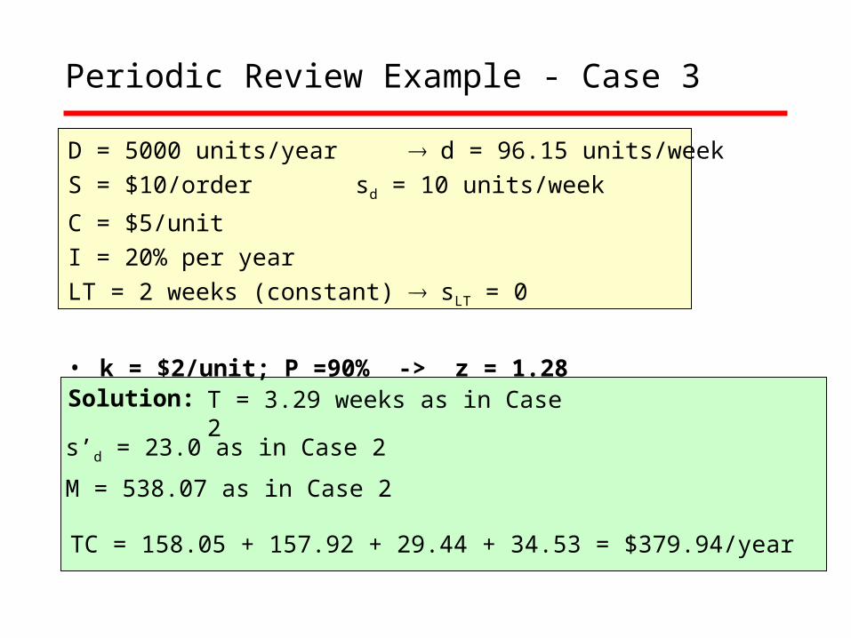
Periodic Review Example - Case 3
D = 5000 units/year d = 96.15 units/weekS = $10/order sd = 10 units/week
C = $5/unitI = 20% per yearLT = 2 weeks (constant) sLT = 0
• k = $2/unit; P =90% -> z = 1.28
T = 3.29 weeks as in Case 2Solution:
TC = 158.05 + 157.92 + 29.44 + 34.53 = $379.94/year
s’d = 23.0 as in Case 2
M = 538.07 as in Case 2
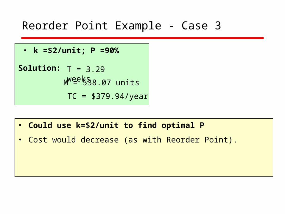
Reorder Point Example - Case 3
• k =$2/unit; P =90%
T = 3.29 weeksSolution:
TC = $379.94/year
M = 538.07 units
• Could use k=$2/unit to find optimal P
• Cost would decrease (as with Reorder Point).
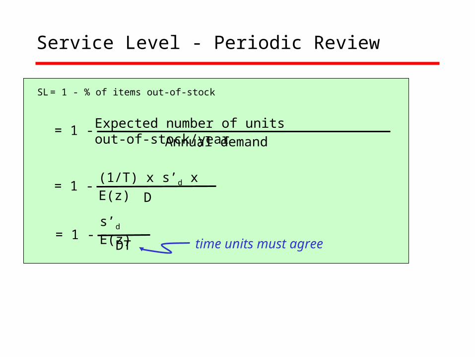
Expected number of units out-of-stock/year
Service Level - Periodic Review
Annual demand
SL= 1 - % of items out-of-stock
= 1 -
(1/T) x s’d x E(z)
D= 1 -
s’d E(z)
DT= 1 -
time units must agree
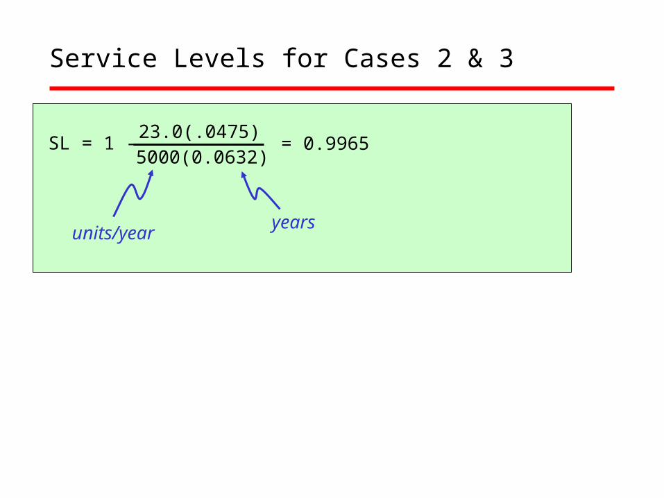
Service Levels for Cases 2 & 3
SL = 1 -23.0(.0475)5000(0.0632)
= 0.9965
units/yearyears
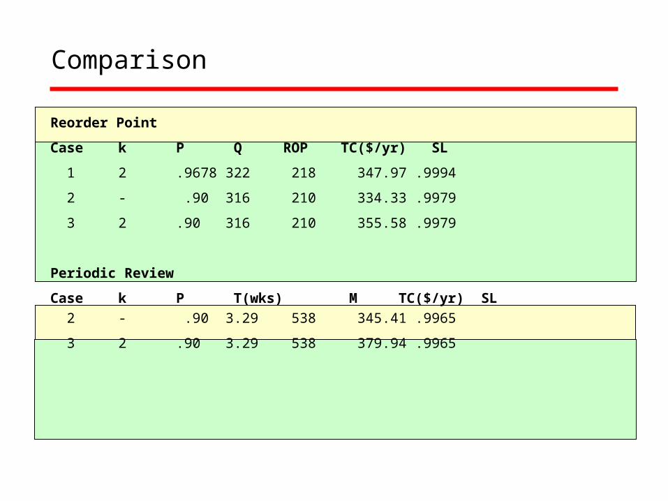
Comparison
Reorder Point
Case k P Q ROP TC($/yr) SL
1 2 .9678 322 218 347.97 .9994
2 - .90 316 210 334.33 .9979
3 2 .90 316 210 355.58 .9979
Periodic Review
Case k P T(wks) M TC($/yr) SL 2 - .90 3.29 538 345.41 .9965
3 2 .90 3.29 538 379.94 .9965
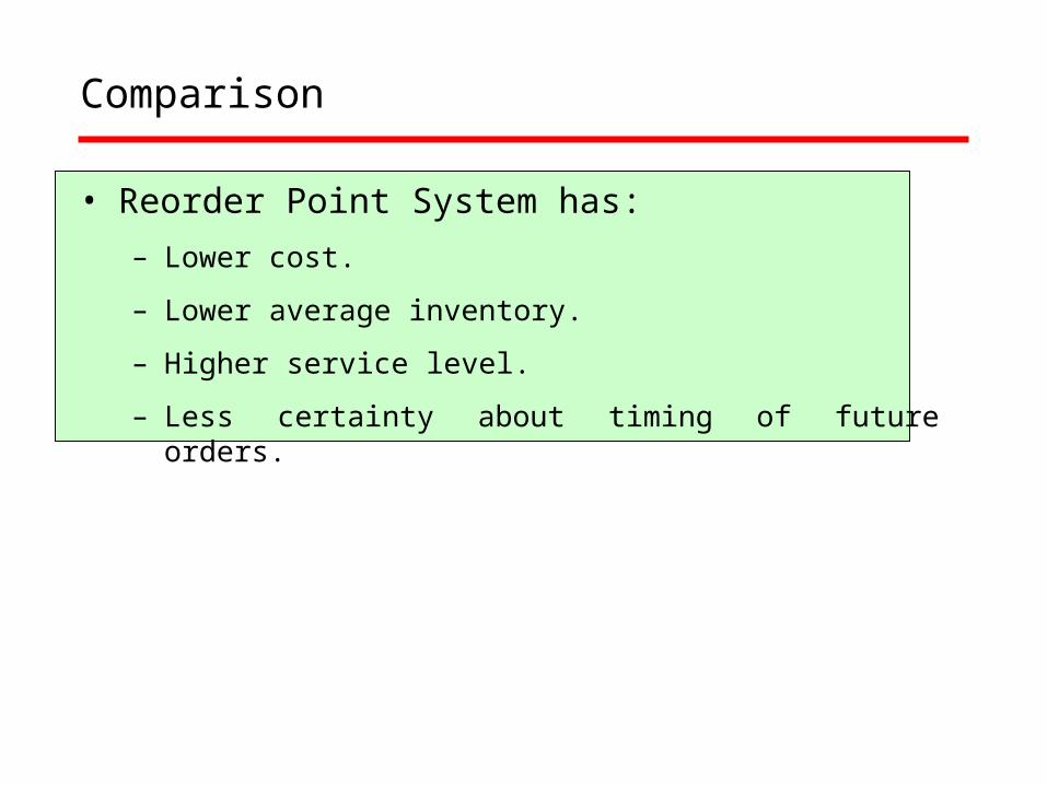
Comparison
• Reorder Point System has:
– Lower cost.
– Lower average inventory.
– Higher service level.
– Less certainty about timing of future orders.
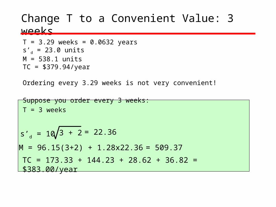
Change T to a Convenient Value: 3 weeks
T = 3.29 weeks = 0.0632 yearss’d = 23.0 unitsM = 538.1 unitsTC = $379.94/year
Ordering every 3.29 weeks is not very convenient!
Suppose you order every 3 weeks:T = 3 weeks
TC = 173.33 + 144.23 + 28.62 + 36.82 = $383.00/year
M = 96.15(3+2) + 1.28x22.36 = 509.37
3 + 2s’d = 10 = 22.36
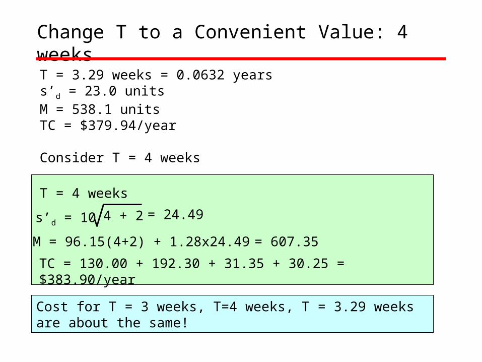
Change T to a Convenient Value: 4 weeks
T = 3.29 weeks = 0.0632 yearss’d = 23.0 unitsM = 538.1 unitsTC = $379.94/year
Consider T = 4 weeks
T = 4 weeks
TC = 130.00 + 192.30 + 31.35 + 30.25 = $383.90/year
M = 96.15(4+2) + 1.28x24.49 = 607.35
4 + 2s’d = 10 = 24.49
Cost for T = 3 weeks, T=4 weeks, T = 3.29 weeks are about the same!
Joint Ordering
• Suppose several items are ordered from the same supplier.
• Each items would have an optimal order interval T.
• This would require frequent orders to the same supplier.
Alternative:
Find a common order interval T and order all items from the same supplier together.
- This is a variation of the periodic review system.
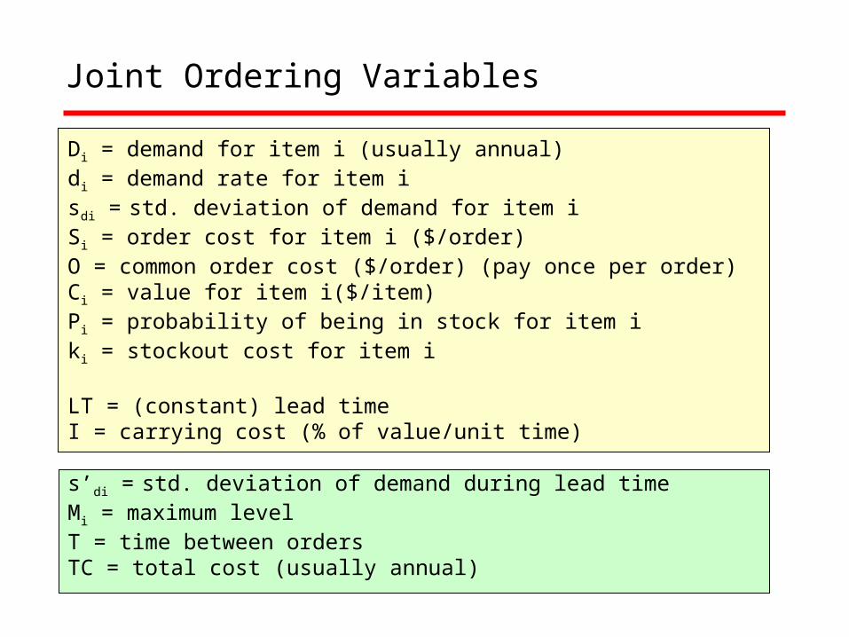
Di = demand for item i (usually annual)di = demand rate for item isdi = std. deviation of demand for item iSi = order cost for item i ($/order)O = common order cost ($/order) (pay once per order)Ci = value for item i($/item) Pi = probability of being in stock for item iki = stockout cost for item i
LT = (constant) lead time I = carrying cost (% of value/unit time)
s’di = std. deviation of demand during lead timeMi = maximum levelT = time between ordersTC = total cost (usually annual)
Joint Ordering Variables
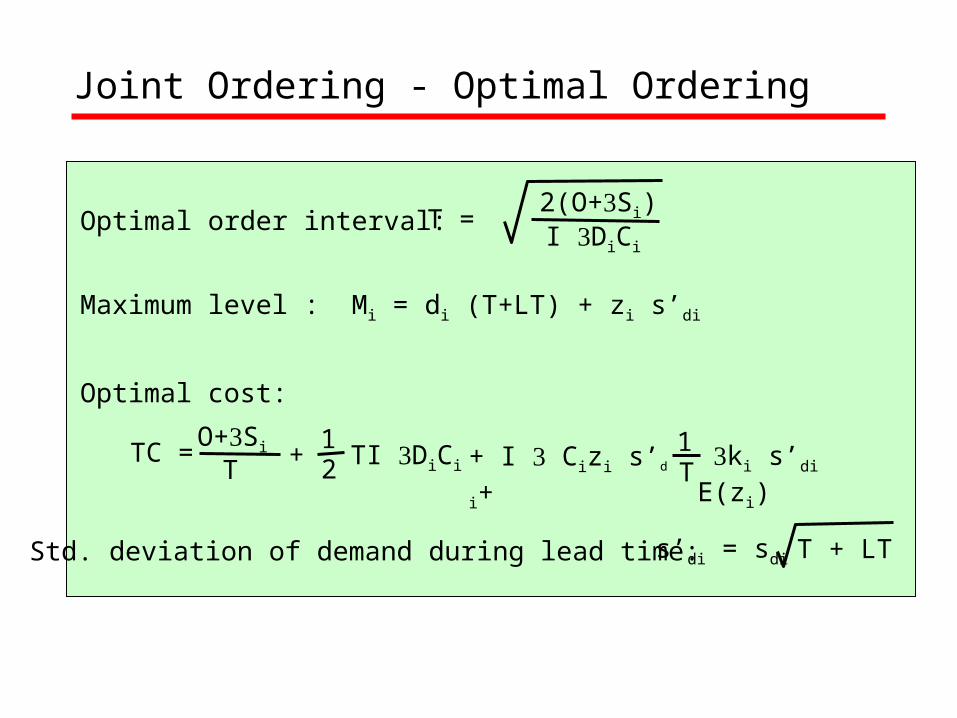
Joint Ordering - Optimal Ordering
Optimal order interval:
Maximum level : Mi = di (T+LT) + zi s’di
Optimal cost:
2(O+Si)T =I DiCi
TC =T
O+Si TI DiCi21
+ I Cizi s’d i+ T1 ki s’di E(zi)
T + LTs’di = sdiStd. deviation of demand during lead time:
+
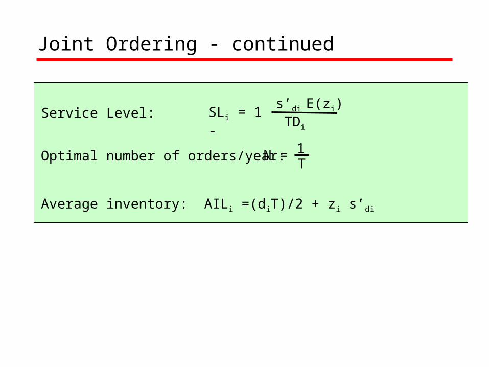
Joint Ordering - continued
Service Level:
Optimal number of orders/year:
Average inventory: AILi =(diT)/2 + zi s’di
s’di E(zi)SLi = 1 -TDi
T1N =
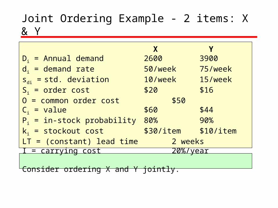
X YDi = Annual demand 2600 3900di = demand rate 50/week 75/weeksdi = std. deviation 10/week 15/weekSi = order cost $20 $16O = common order cost $50Ci = value $60 $44Pi = in-stock probability 80% 90%ki = stockout cost $30/item $10/itemLT = (constant) lead time 2 weeksI = carrying cost 20%/year
Consider ordering X and Y jointly.
Joint Ordering Example - 2 items: X & Y
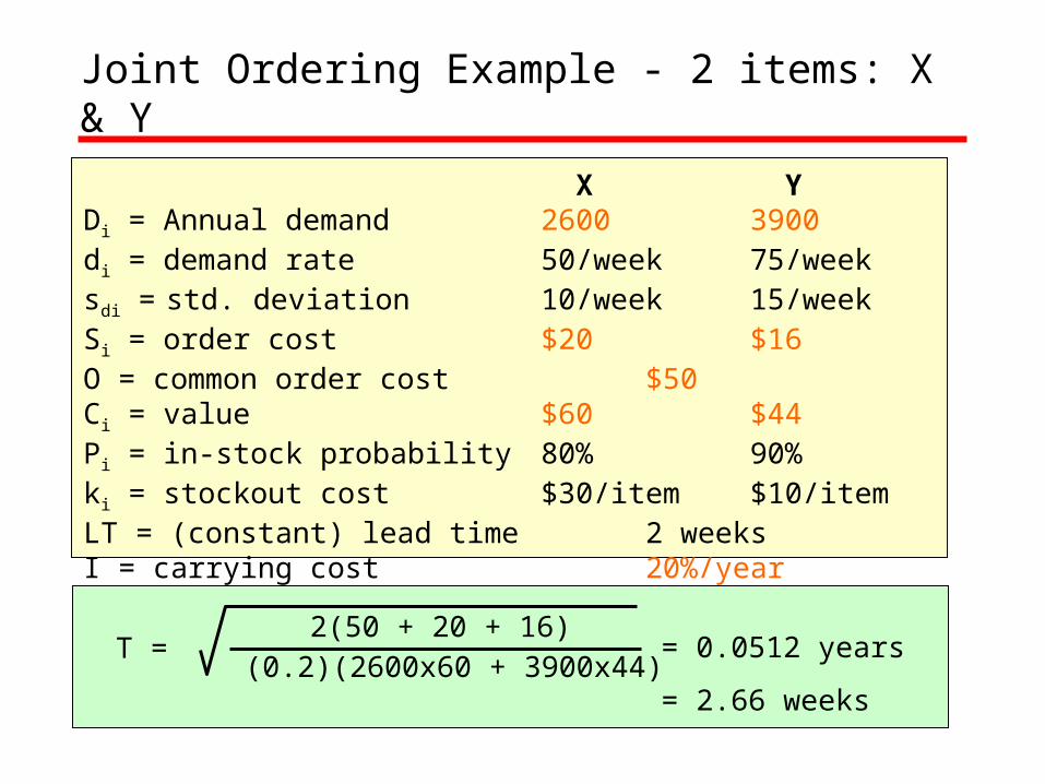
X YDi = Annual demand 2600 3900di = demand rate 50/week 75/weeksdi = std. deviation 10/week 15/weekSi = order cost $20 $16O = common order cost $50Ci = value $60 $44Pi = in-stock probability 80% 90%ki = stockout cost $30/item $10/itemLT = (constant) lead time 2 weeksI = carrying cost 20%/year
Joint Ordering Example - 2 items: X & Y
2(50 + 20 + 16)T =
(0.2)(2600x60 + 3900x44)= 0.0512 years
= 2.66 weeks
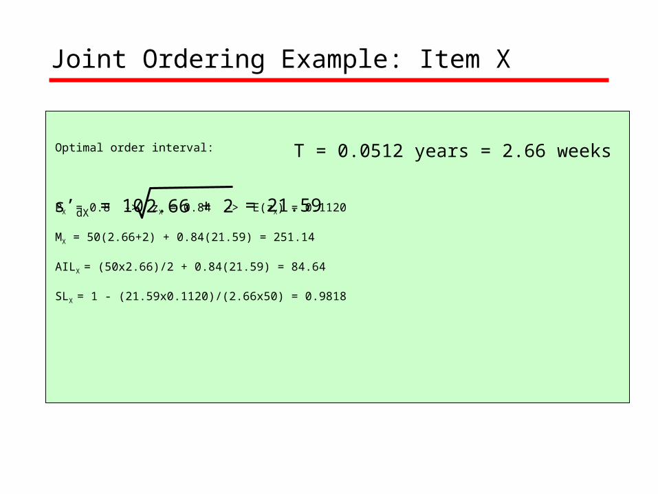
Joint Ordering Example: Item X
Optimal order interval:
PX = 0.8 -> zX = 0.84 -> E(zX) = 0.1120
MX = 50(2.66+2) + 0.84(21.59) = 251.14
AILX = (50x2.66)/2 + 0.84(21.59) = 84.64
SLX = 1 - (21.59x0.1120)/(2.66x50) = 0.9818
T = 0.0512 years = 2.66 weeks
2.66 + 2s’dX = 10 = 21.59

Joint Ordering Example: Item Y
Optimal order interval:
PY = 0.9 -> zY = 1.28 -> E(zY) = 0.0475
MY = 75(2.66+2) + 1.28(32.38) = 390.95
AILY = (75x2.66)/2 + 1.28(32.38) = 141.20
SLY = 1 - (32.38x0.0475)/(2.66x75) = 0.9923
T = 0.0512 years = 2.66 weeks
2.66 + 2s’dY = 15 = 32.38
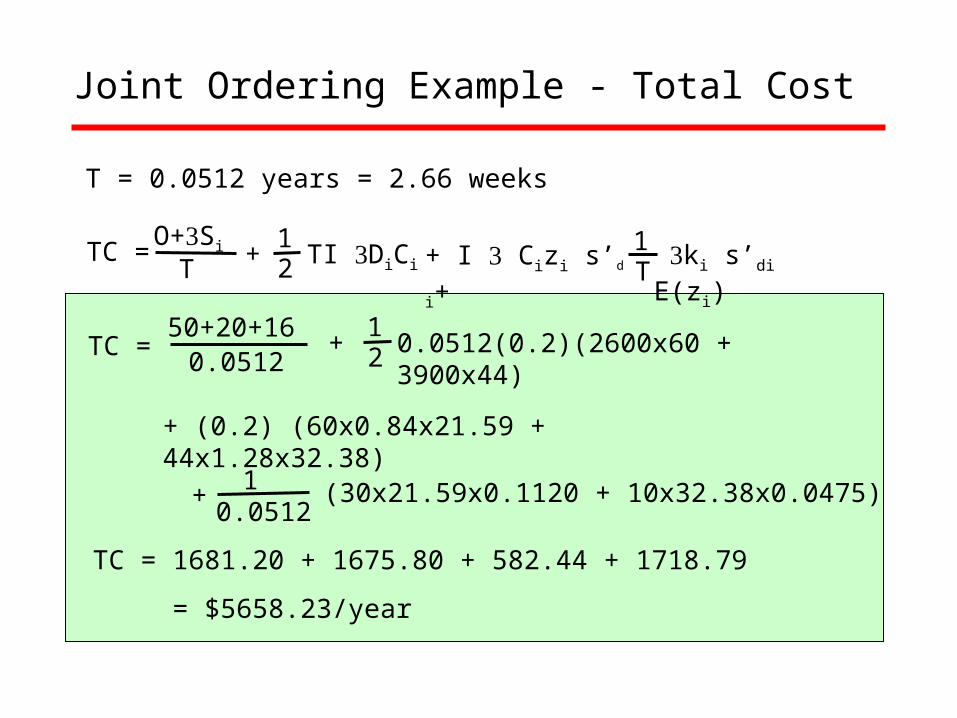
Joint Ordering Example - Total Cost
T = 0.0512 years = 2.66 weeks
TC =0.0512
50+20+160.0512(0.2)(2600x60 + 3900x44)2
1
+ (0.2) (60x0.84x21.59 + 44x1.28x32.38)
0.05121 (30x21.59x0.1120 + 10x32.38x0.0475)
+
TC =T
O+Si TI DiCi21
+ I Cizi s’d i+ T1 ki s’di E(zi) +
+
TC = 1681.20 + 1675.80 + 582.44 + 1718.79
= $5658.23/year
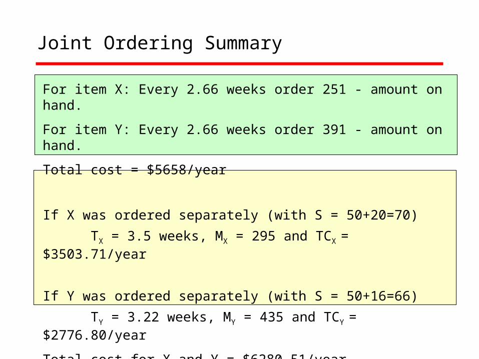
Joint Ordering Summary
For item X: Every 2.66 weeks order 251 - amount on hand.
For item Y: Every 2.66 weeks order 391 - amount on hand.
Total cost = $5658/year
If X was ordered separately (with S = 50+20=70)
TX = 3.5 weeks, MX = 295 and TCX = $3503.71/year
If Y was ordered separately (with S = 50+16=66)
TY = 3.22 weeks, MY = 435 and TCY = $2776.80/year
Total cost for X and Y = $6280.51/year
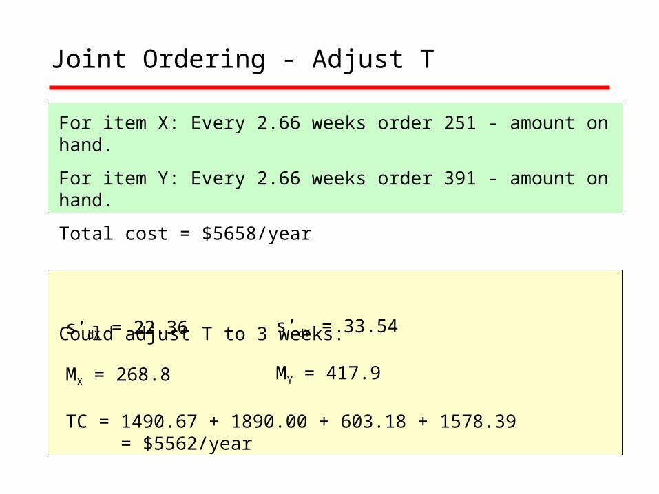
Joint Ordering - Adjust T
For item X: Every 2.66 weeks order 251 - amount on hand.
For item Y: Every 2.66 weeks order 391 - amount on hand.
Total cost = $5658/year
Could adjust T to 3 weeks:
s’dX = 22.36
MX = 268.8
TC = 1490.67 + 1890.00 + 603.18 + 1578.39 = $5562/year
s’dY = 33.54
MY = 417.9
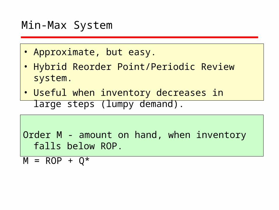
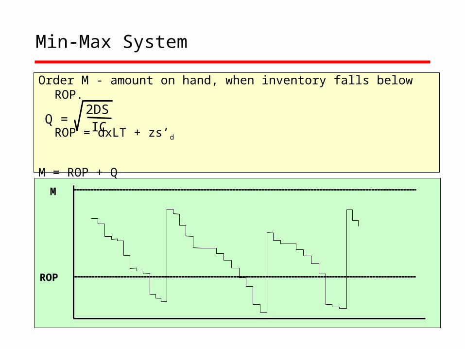
Min-Max System
• Approximate, but easy.
• Hybrid Reorder Point/Periodic Review system.
• Useful when inventory decreases in large steps (lumpy demand).
Order M - amount on hand, when inventory falls below ROP.
M = ROP + Q*
Min-Max System
Order M - amount on hand, when inventory falls below ROP.
ROP = dxLT + zs’d
M = ROP + Q
Q =IC
2DS
ROP
M
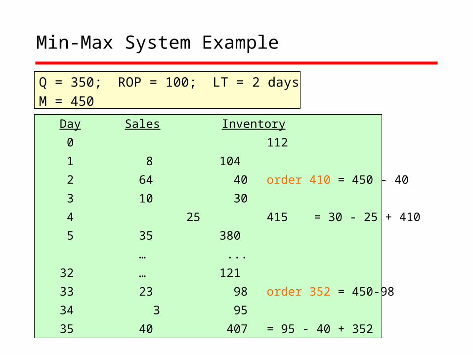
Min-Max System Example
Q = 350; ROP = 100; LT = 2 daysM = 450
Day Sales Inventory
0 112
1 8 104
2 64 40 order 410 = 450 - 40
3 10 30
4 25 415 = 30 - 25 + 410
5 35 380
… ...
32 … 121
33 23 98 order 352 = 450-98
34 3 95
35 40 407 = 95 - 40 + 352
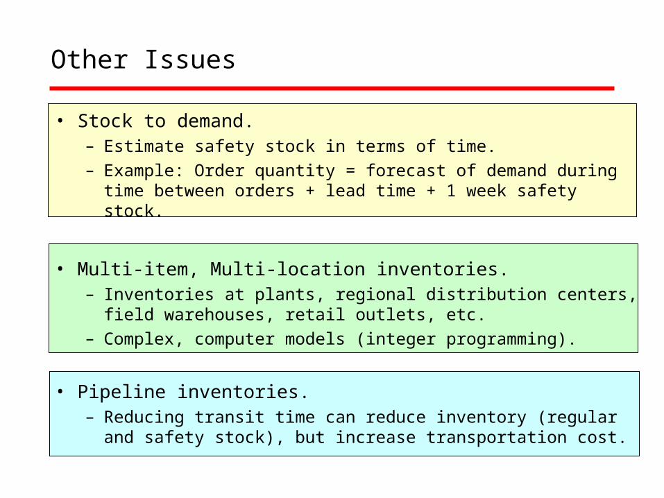
Other Issues
• Stock to demand.– Estimate safety stock in terms of time.– Example: Order quantity = forecast of demand during
time between orders + lead time + 1 week safety stock.
• Multi-item, Multi-location inventories.– Inventories at plants, regional distribution centers, field
warehouses, retail outlets, etc.– Complex, computer models (integer programming).
• Pipeline inventories.– Reducing transit time can reduce inventory (regular and
safety stock), but increase transportation cost.
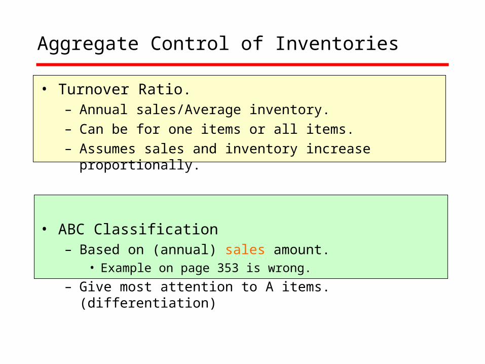
Aggregate Control of Inventories
• Turnover Ratio.– Annual sales/Average inventory.– Can be for one items or all items.– Assumes sales and inventory increase proportionally.
• ABC Classification– Based on (annual) sales amount.
• Example on page 353 is wrong.
– Give most attention to A items. (differentiation)
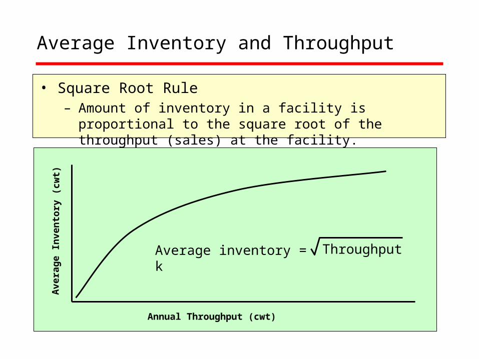
Average Inventory and Throughput
• Square Root Rule– Amount of inventory in a facility is proportional to the
square root of the throughput (sales) at the facility.
Annual Throughput (cwt)
Avera
ge I
nven
tory
(cw
t)
Average inventory = k Throughput
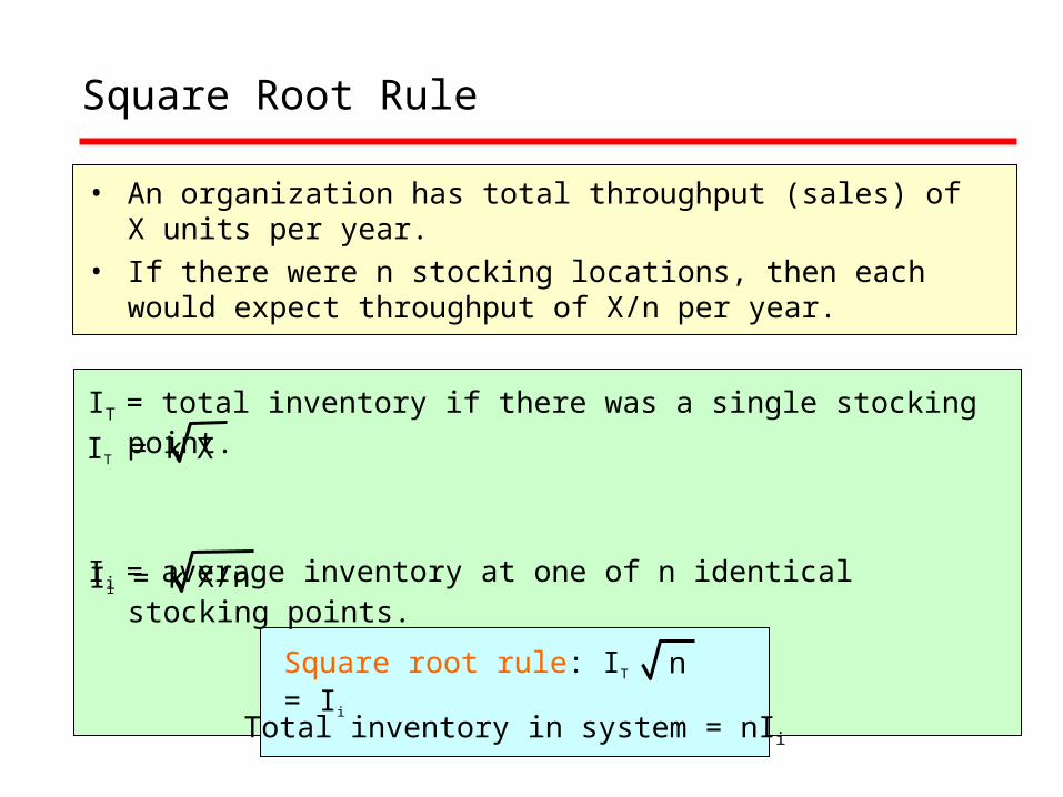
Square Root Rule
• An organization has total throughput (sales) of X units per year.
• If there were n stocking locations, then each would expect throughput of X/n per year.
IT = total inventory if there was a single stocking point.
Ii = average inventory at one of n identical stocking points.
IT = k X
Ii = k X/n
Square root rule: IT = Ii n
Total inventory in system = nIi
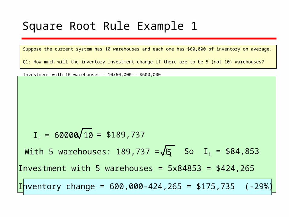
Square Root Rule Example 1
Suppose the current system has 10 warehouses and each one has $60,000 of inventory on average.
Q1: How much will the inventory investment change if there are to be 5 (not 10) warehouses?
Investment with 10 warehouses = 10x60,000 = $600,000
IT = 60000 10 = $189,737
With 5 warehouses: 189,737 = Ii 5
Investment with 5 warehouses = 5x84853 = $424,265
So Ii = $84,853
Inventory change = 600,000-424,265 = $175,735 (-29%)
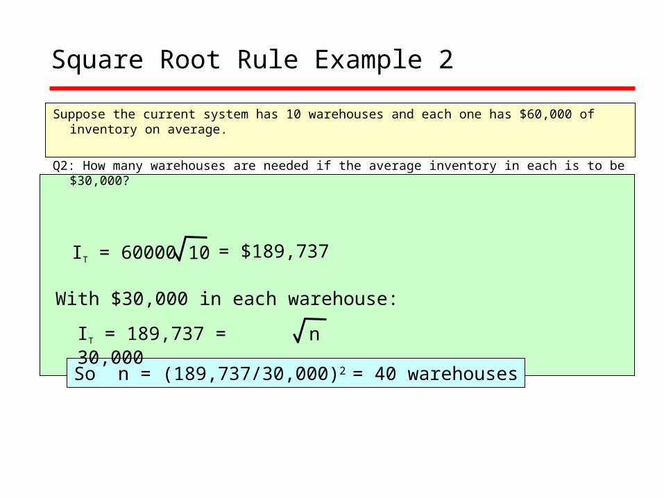
Square Root Rule Example 2
Suppose the current system has 10 warehouses and each one has $60,000 of inventory on average.
Q2: How many warehouses are needed if the average inventory in each is to be $30,000?
IT = 60000 10 = $189,737
With $30,000 in each warehouse:
n
So n = (189,737/30,000)2 = 40 warehouses
IT = 189,737 = 30,000
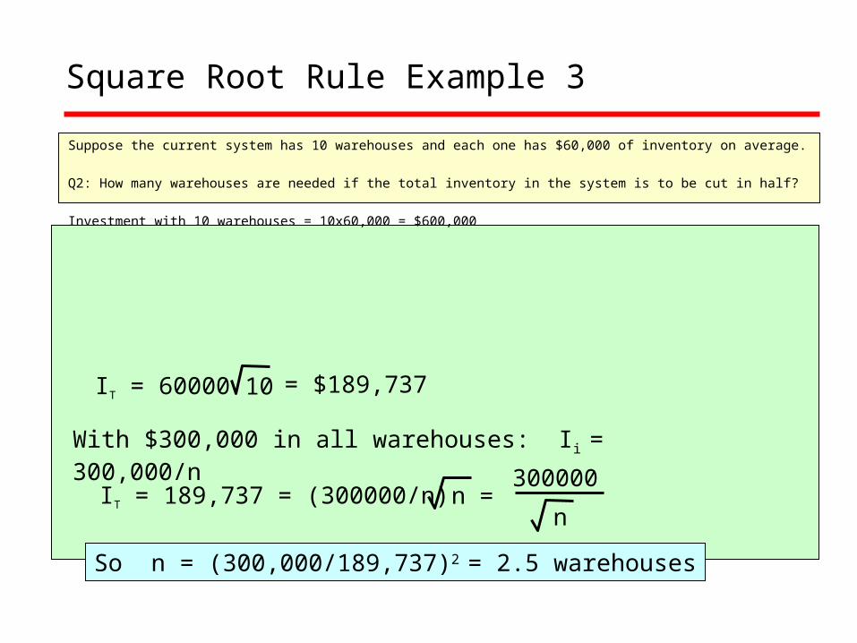
Square Root Rule Example 3
Suppose the current system has 10 warehouses and each one has $60,000 of inventory on average.
Q2: How many warehouses are needed if the total inventory in the system is to be cut in half? Investment with 10 warehouses = 10x60,000 = $600,000
IT = 60000 10 = $189,737
With $300,000 in all warehouses: Ii = 300,000/n
n
So n = (300,000/189,737)2 = 2.5 warehouses
IT = 189,737 = (300000/n) n
300000=
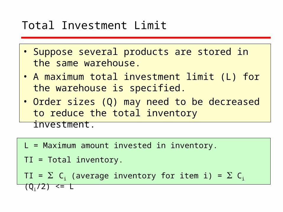
Total Investment Limit
• Suppose several products are stored in the same warehouse.
• A maximum total investment limit (L) for the warehouse is specified.
• Order sizes (Q) may need to be decreased to reduce the total inventory investment.
L = Maximum amount invested in inventory.
TI = Total inventory.
TI = Ci (average inventory for item i) = Ci (Qi/2) <= L
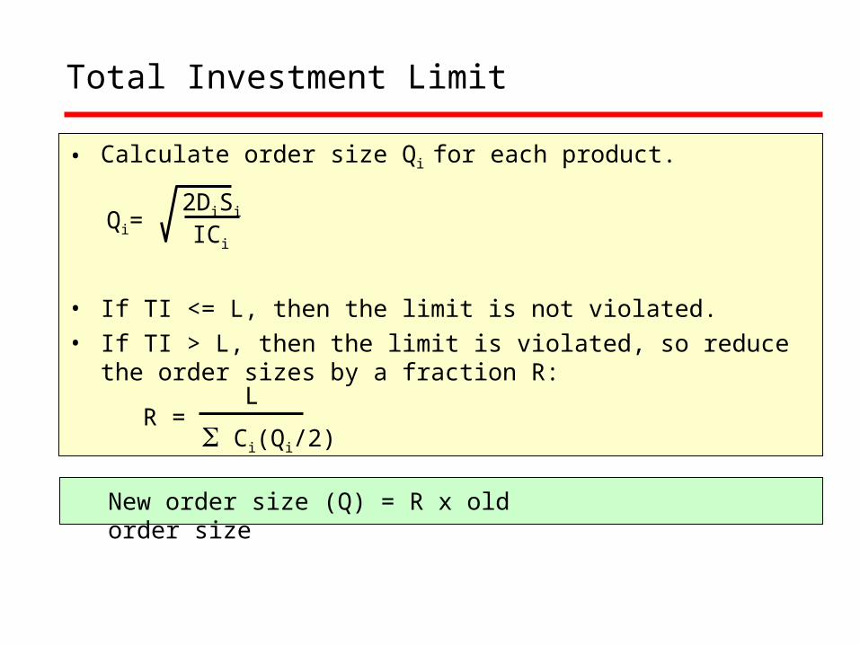
Total Investment Limit
• Calculate order size Qi for each product.
• If TI <= L, then the limit is not violated.• If TI > L, then the limit is violated, so reduce the order
sizes by a fraction R:
Qi= ICi
2DiSi
R =
L
Ci(Qi/2)
New order size (Q) = R x old order size
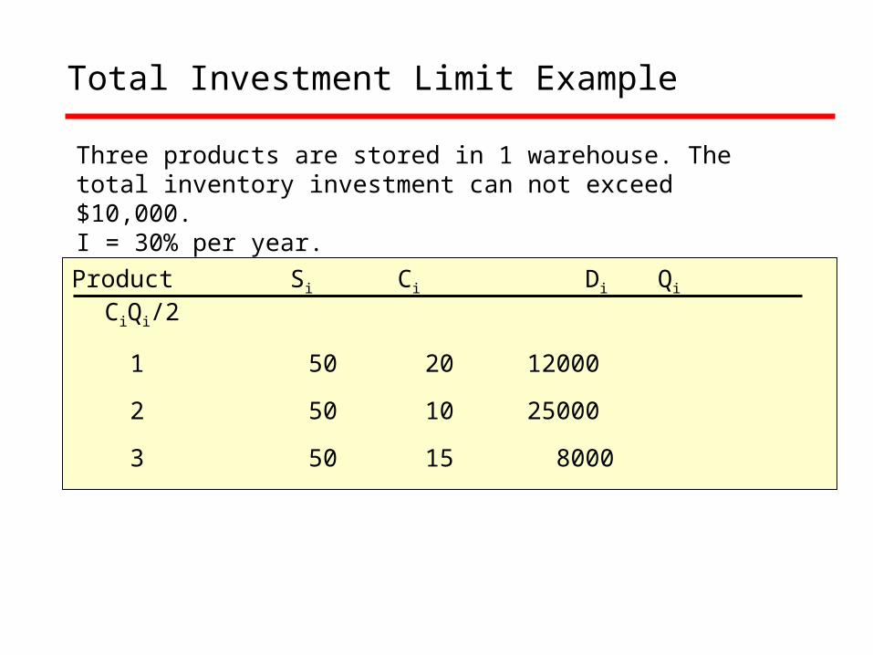
Total Investment Limit Example
Product Si Ci Di Qi CiQi/2
1 50 20 12000
2 50 10 25000
3 50 15 8000
Three products are stored in 1 warehouse. The total inventory investment can not exceed $10,000.I = 30% per year.
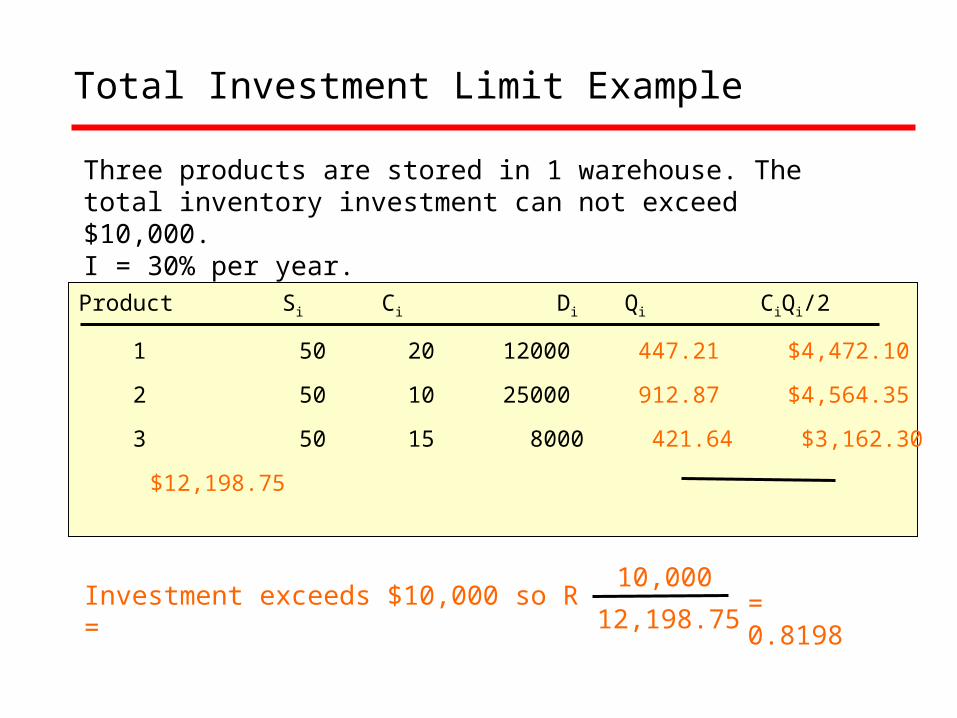
Total Investment Limit Example
Product Si Ci Di Qi CiQi/2
1 50 20 12000 447.21 $4,472.10
2 50 10 25000 912.87 $4,564.35
3 50 15 8000 421.64 $3,162.30
$12,198.75
Investment exceeds $10,000 so R =
10,000
12,198.75
Three products are stored in 1 warehouse. The total inventory investment can not exceed $10,000.I = 30% per year.
= 0.8198
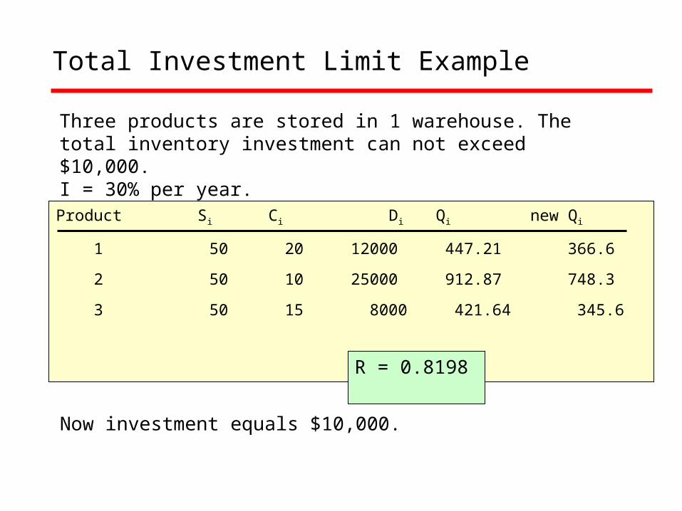
Total Investment Limit Example
Product Si Ci Di Qi new Qi
1 50 20 12000 447.21 366.6
2 50 10 25000 912.87 748.3
3 50 15 8000 421.64 345.6
Now investment equals $10,000.
Three products are stored in 1 warehouse. The total inventory investment can not exceed $10,000.I = 30% per year.
R = 0.8198
Just-In-Time (JIT)
• Production system that originated in Japan.• Toyota is best known example.• Now used by many U.S. manufacturers and
suppliers.
• Producer: Produce small lots of high quality products with low inventory.
• Supplier: Deliver small lots of high quality components on time.
Just-In-Time Goals
• Philosophy:– Synchronize the supply chain to respond to customers.– Eliminate all waste (inventory and scrap).
• Goals:– Zero inventory.– Lot size of 1.– 100% quality.
• Continuously strive to reduce inventory and lot size - and improve quality.
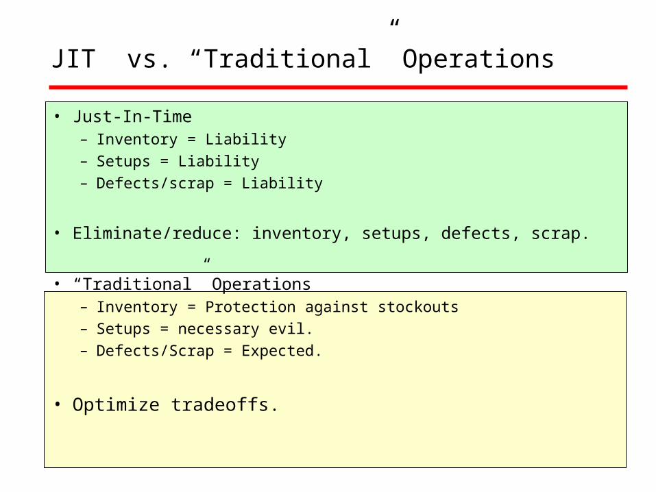
JIT vs. “Traditional” Operations
• Just-In-Time– Inventory = Liability – Setups = Liability– Defects/scrap = Liability
• Eliminate/reduce: inventory, setups, defects, scrap.
• “Traditional” Operations– Inventory = Protection against stockouts– Setups = necessary evil.– Defects/Scrap = Expected.
• Optimize tradeoffs.
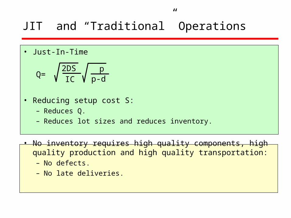
JIT and “Traditional” Operations
• Just-In-Time
• Reducing setup cost S:– Reduces Q.– Reduces lot sizes and reduces inventory.
• No inventory requires high quality components, high quality production and high quality transportation:– No defects.– No late deliveries.
Q=IC
2DSp-d p
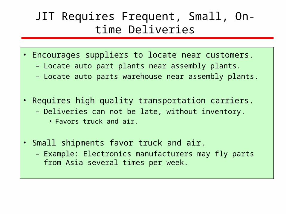
JIT Requires Frequent, Small, On-time Deliveries
• Encourages suppliers to locate near customers.– Locate auto part plants near assembly plants.– Locate auto parts warehouse near assembly plants.
• Requires high quality transportation carriers.– Deliveries can not be late, without inventory.
• Favors truck and air.
• Small shipments favor truck and air.– Example: Electronics manufacturers may fly parts
from Asia several times per week.
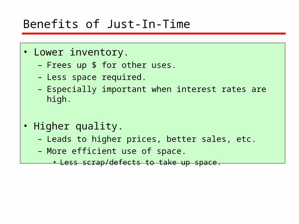
Benefits of Just-In-Time
• Lower inventory.– Frees up $ for other uses.– Less space required.– Especially important when interest rates are high.
• Higher quality.– Leads to higher prices, better sales, etc.– More efficient use of space.
• Less scrap/defects to take up space.
Concerns with Just-In-Time
• Low inventory requires secure, reliable supply chains.– Reliable suppliers and transportation.– Reliable infrastructure.
• Difficult to implement.– Requires major changes in business processes.– Hard to do “partial just-in-time”.– Difficult to phase in.– Works best if suppliers use just-in-time.
Japan and Just-In-Time
• How does Japan differ from the USA?– Area.– Population.– Land use.– Resources.
• What are implications for success of just-in-time?