Chapter 10

Fluids

Fluids in Motion

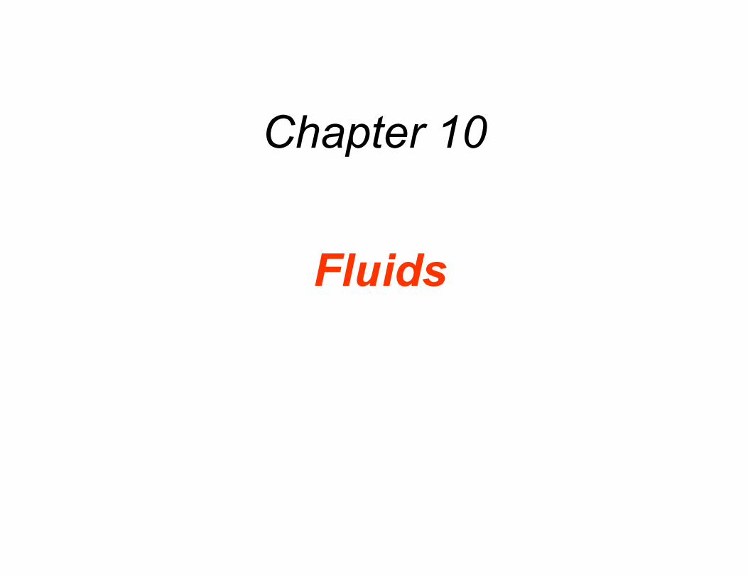
In steady flow the velocity of the fluid particles at any point is constant as time passes.

Unsteady flow exists whenever the velocity of the fluid particles at a point changes as time passes.

Turbulent flow is an extreme kind of unsteady flow in which the velocity of the fluid particles at a point change erratically in both magnitude and direction.

Fluids in Motion

Fluid flow can be compressible or incompressible. Most liquids are nearly incompressible. Fluid flow can be viscous such that the fluid does not flow readily due to internal frictional forces being present (e.g. honey), or nonviscous such that the fluid flows readily due to no internal frictional forces being present (e.g. water is almost nonviscous). An incompressible, nonviscous fluid is called an ideal fluid.

Fluids in Motion

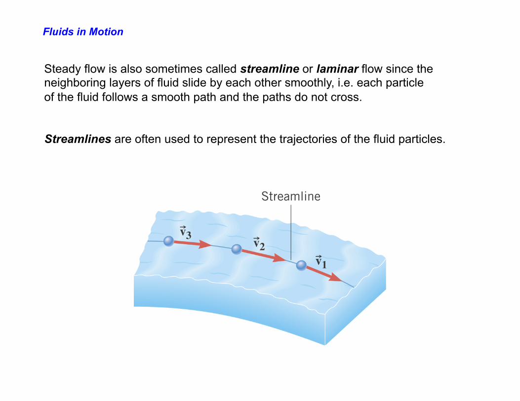
Steady flow is also sometimes called streamline or laminar flow since the neighboring layers of fluid slide by each other smoothly, i.e. each particle of the fluid follows a smooth path and the paths do not cross. Streamlines are often used to represent the trajectories of the fluid particles.

Fluids in Motion

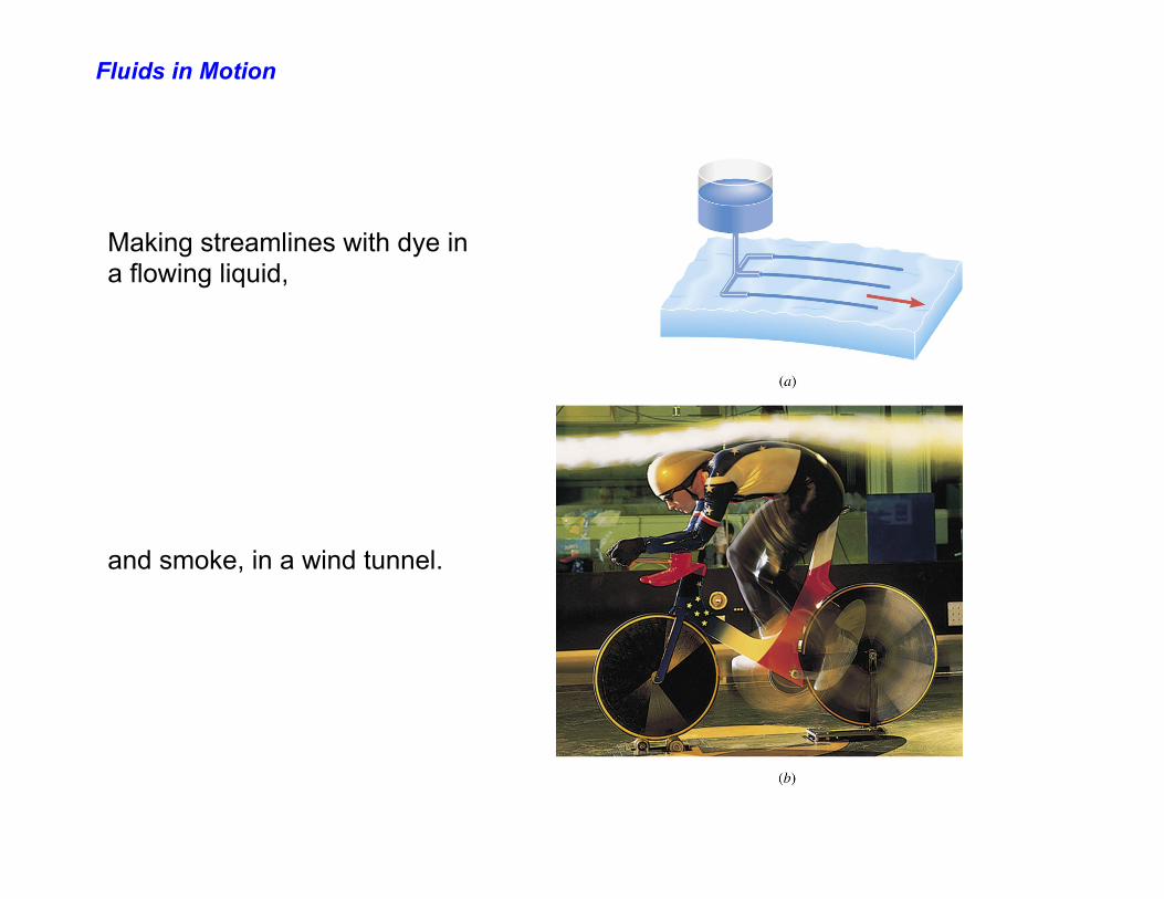
Making streamlines with dye in a flowing liquid, and smoke, in a wind tunnel.

The Equation of Continuity

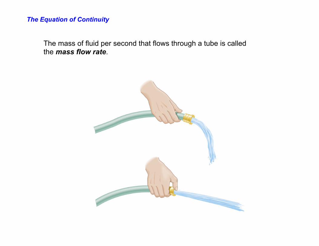
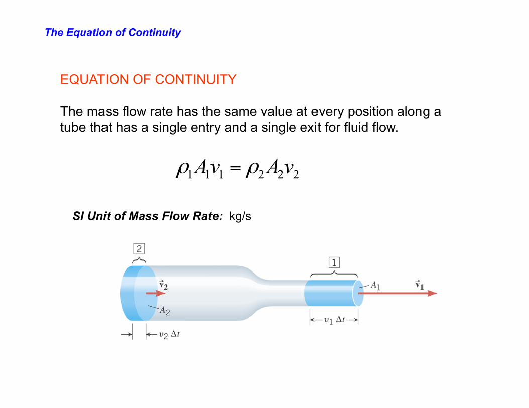
The mass of fluid per second that flows through a tube is called the mass flow rate.

The Equation of Continuity

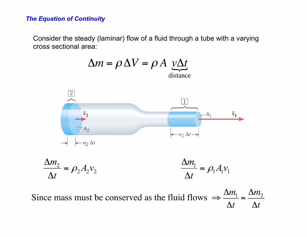
2222 vAtm

ρ=Δ

Δ111

1 vAtm

ρ=Δ

Δ

Δm = ρΔV = ρ A vΔtdistance!

Consider the steady (laminar) flow of a fluid through a tube with a varying cross sectional area:

Since mass must be conserved as the fluid flows ⇒ Δm1

Δt=Δm2

Δt

The Equation of Continuity

222111 vAvA ρρ =

EQUATION OF CONTINUITY The mass flow rate has the same value at every position along a tube that has a single entry and a single exit for fluid flow.

SI Unit of Mass Flow Rate: kg/s

The Equation of Continuity

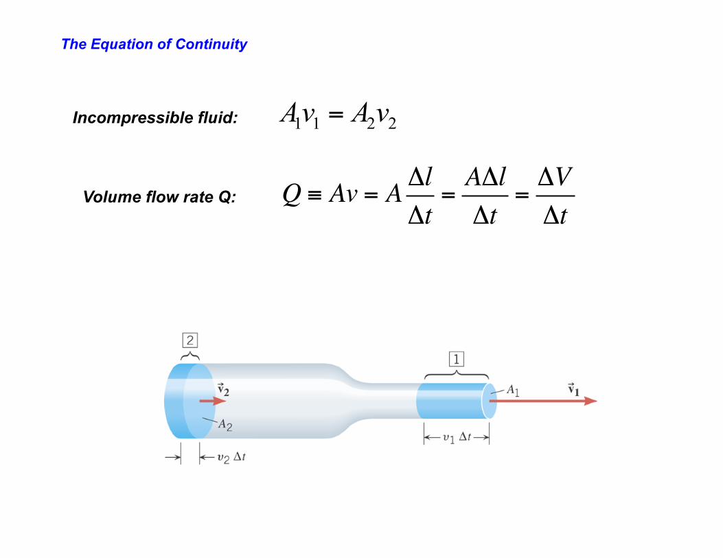
Incompressible fluid: 2211 vAvA =

Volume flow rate Q: Q ≡ Av = A ΔlΔt

=AΔlΔt

=ΔVΔt

The Equation of Continuity

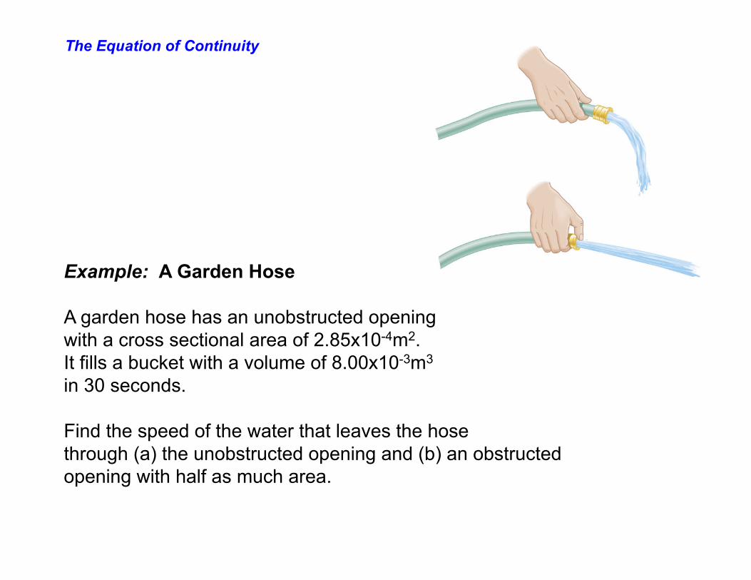
Example: A Garden Hose A garden hose has an unobstructed opening with a cross sectional area of 2.85x10-4m2. It fills a bucket with a volume of 8.00x10-3m3 in 30 seconds. Find the speed of the water that leaves the hose through (a) the unobstructed opening and (b) an obstructed opening with half as much area.

The Equation of Continuity

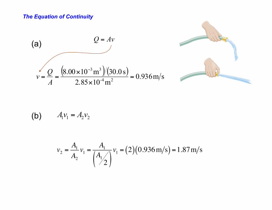
AvQ =

( ) ( ) sm936.0m102.85

s 30.0m1000.824-

33

=×

×==

−

AQv

(a)

(b) 2211 vAvA =

v2 =A1A2v1 =

A1A12( )v1 = 2( ) 0.936m s( ) =1.87m s

Bernoulli’s Equation

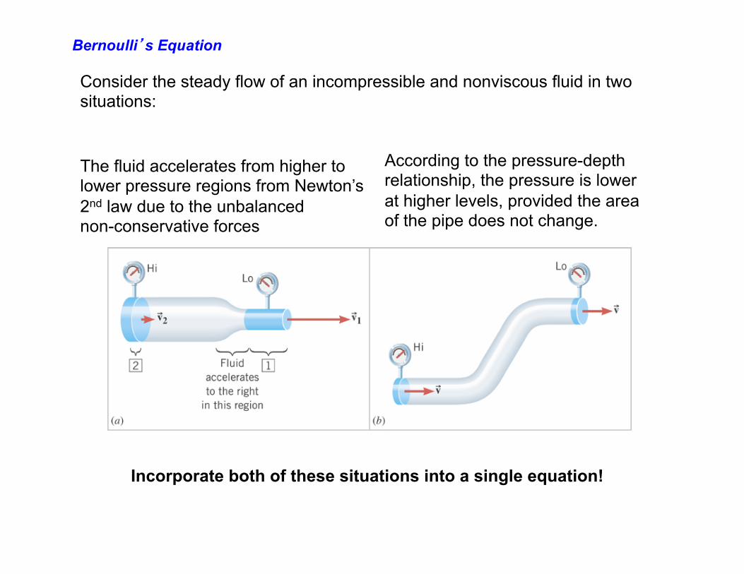
The fluid accelerates from higher to lower pressure regions from Newton’s 2nd law due to the unbalanced non-conservative forces

According to the pressure-depth relationship, the pressure is lower at higher levels, provided the area of the pipe does not change.

Consider the steady flow of an incompressible and nonviscous fluid in two situations:

Incorporate both of these situations into a single equation!

Bernoulli’s Equation

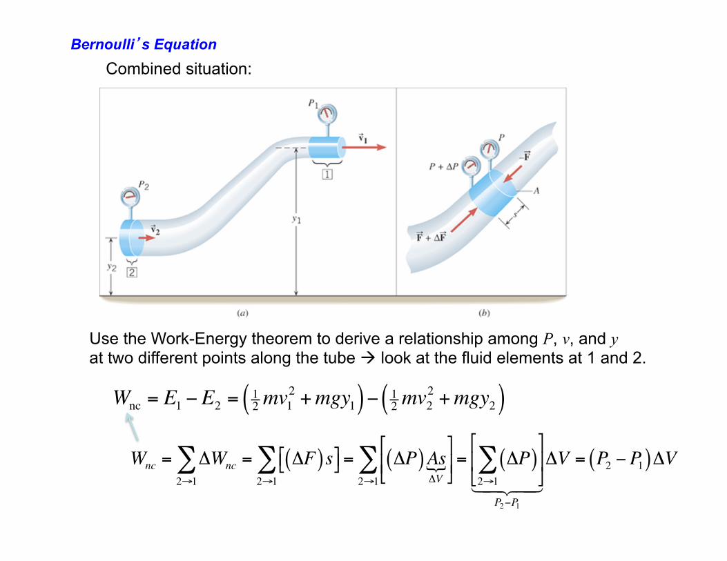
Wnc = E1 −E2 = 12mv1

2 +mgy1( )− 12mv2

2 +mgy2( )

Wnc = ΔWnc = ΔF( )s"# $%2→1∑

2→1∑ = ΔP( )As

ΔV!

"

#($

%)2→1∑ = ΔP( )

2→1∑"

#(

$

%)

P2−P1! "# $#

ΔV = P2 −P1( )ΔV

Combined situation:

Use the Work-Energy theorem to derive a relationship among P, v, and y at two different points along the tube à look at the fluid elements at 1 and 2.

Bernoulli’s Equation

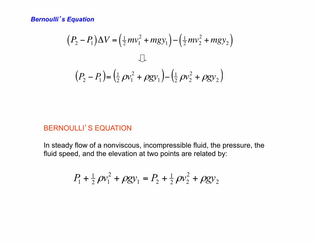
P2 −P1( )ΔV = 12mv1

2 +mgy1( )− 12mv2

2 +mgy2( )

( ) ( ) ( )2222

11

212

112 gyvgyvPP ρρρρ +−+=−

BERNOULLI’S EQUATION In steady flow of a nonviscous, incompressible fluid, the pressure, the fluid speed, and the elevation at two points are related by:

2222

121

212

11 gyvPgyvP ρρρρ ++=++

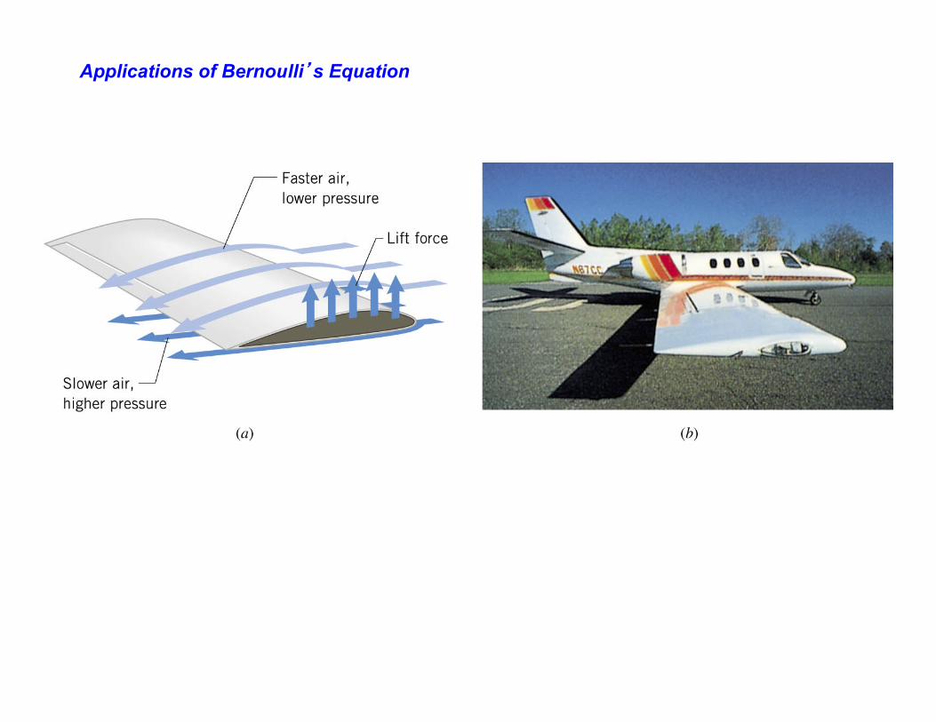
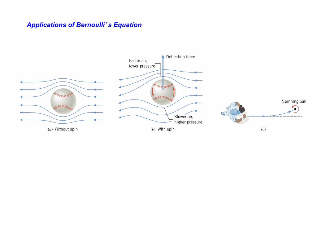
Applications of Bernoulli’s Equation

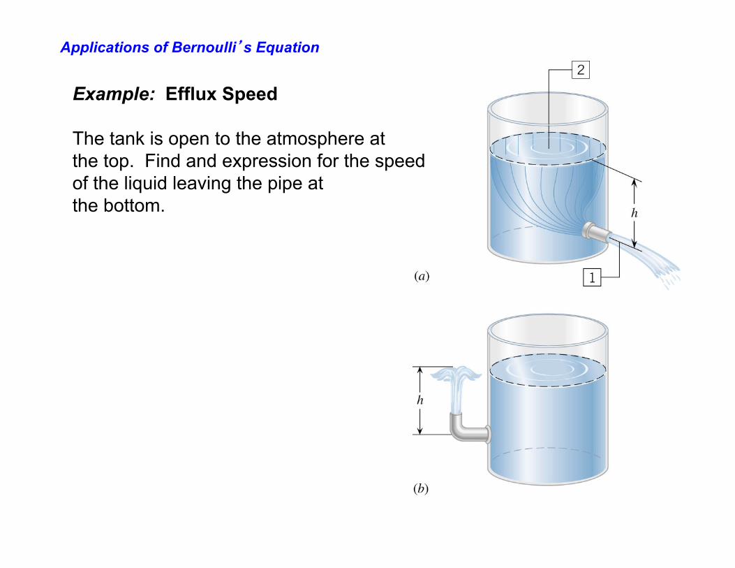
Example: Efflux Speed The tank is open to the atmosphere at the top. Find and expression for the speed of the liquid leaving the pipe at the bottom.

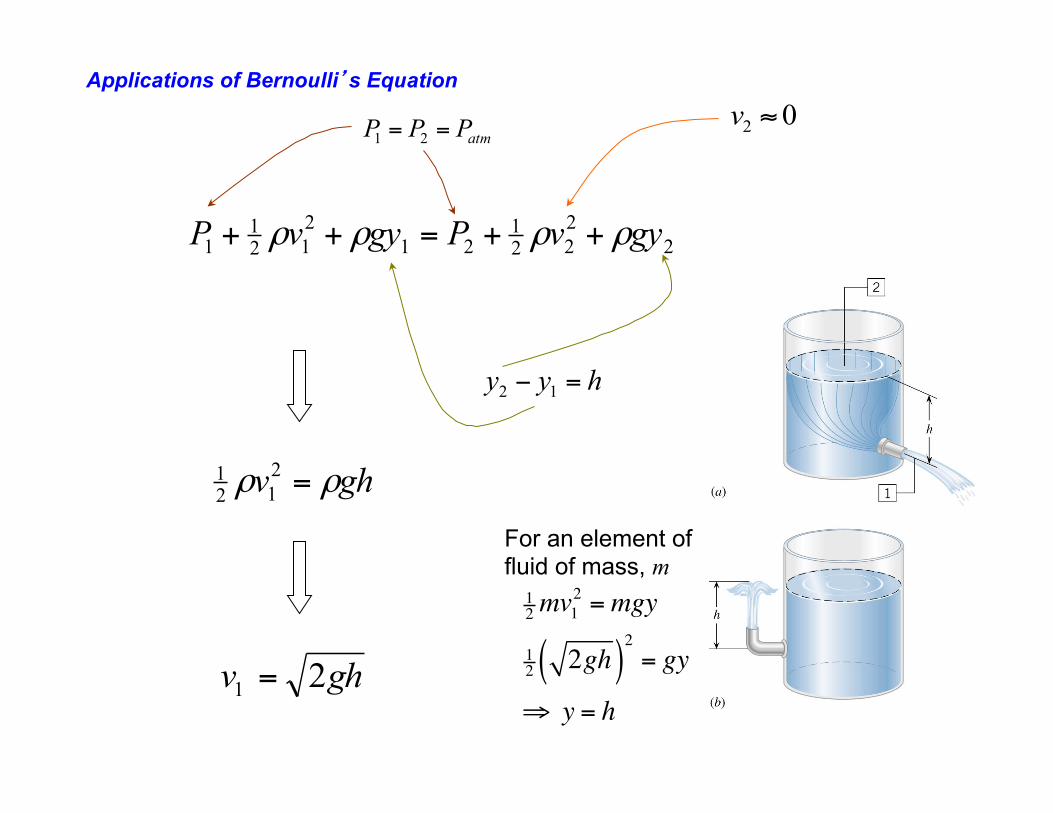
Applications of Bernoulli’s Equation

2222

121

212

11 gyvPgyvP ρρρρ ++=++

atmPPP == 2102 ≈v

hyy =− 12

ghv ρρ =2121

ghv 21 =

For an element of fluid of mass, m 12mv1

2 =mgy

12 2gh( )

2= gy

⇒ y = h

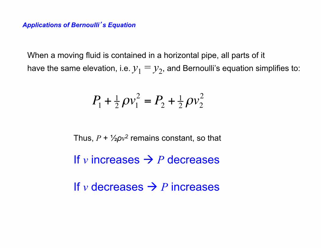
When a moving fluid is contained in a horizontal pipe, all parts of it have the same elevation, i.e. y1 = y2, and Bernoulli’s equation simplifies to:

P1 + 12 ρv1

2 = P2 + 12 ρv2

2

Thus, P + ½ρv2 remains constant, so that If v increases à P decreases If v decreases à P increases

Applications of Bernoulli’s Equation

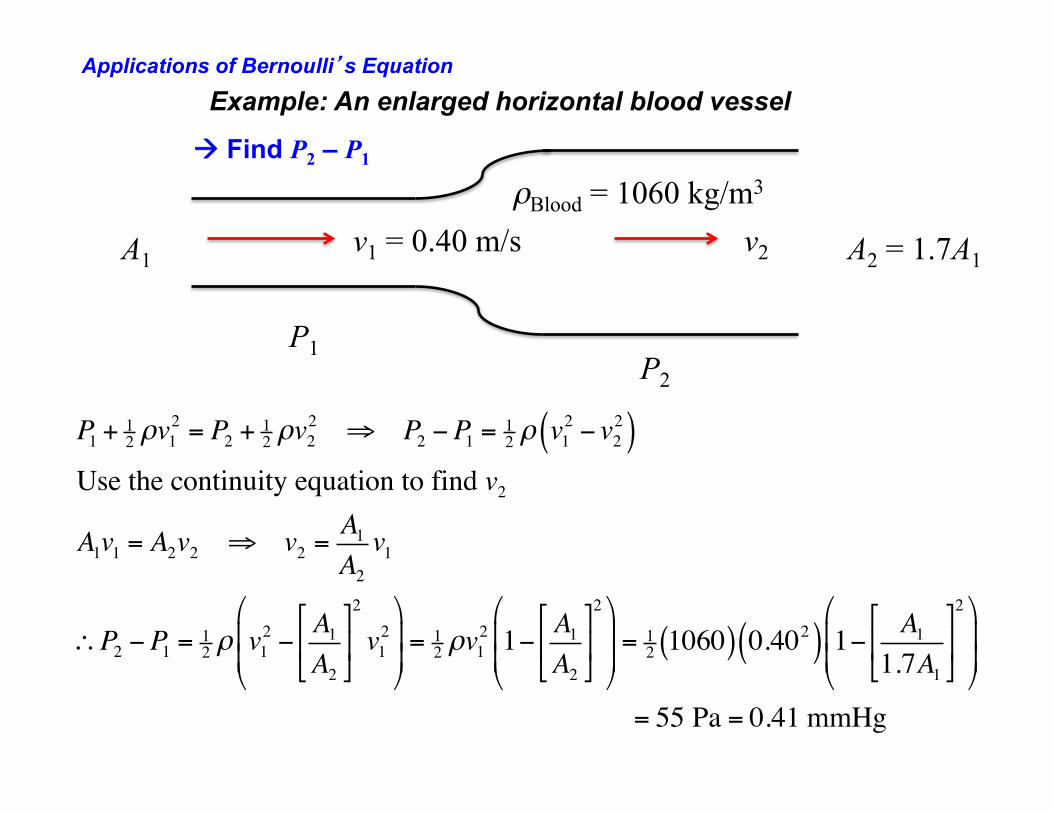
Example: An enlarged horizontal blood vessel

A1 A2 = 1.7A1

P1 P2

v1 = 0.40 m/s v2

à Find P2 – P1

ρBlood = 1060 kg/m3

P1 + 12 ρv1

2 = P2 + 12 ρv2

2 ⇒ P2 −P1 = 12 ρ v1

2 − v22( )

Use the continuity equation to find v2

A1v1 = A2v2 ⇒ v2 =A1

A2

v1

∴P2 −P1 = 12 ρ v1

2 −A1

A2

$

%&

'

()

2

v12

*

+,,

-

.//=

12 ρv1

2 1− A1

A2

$

%&

'

()

2*

+,,

-

.//=

12 1060( ) 0.402( ) 1− A1

1.7A1

$

%&

'

()

2*

+,,

-

.//

= 55 Pa = 0.41 mmHg

Applications of Bernoulli’s Equation

Applications of Bernoulli’s Equation

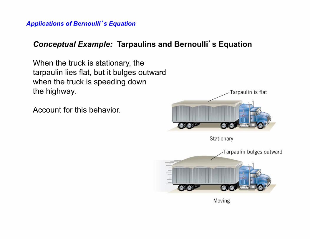
Conceptual Example: Tarpaulins and Bernoulli’s Equation When the truck is stationary, the tarpaulin lies flat, but it bulges outward when the truck is speeding down the highway. Account for this behavior.

Applications of Bernoulli’s Equation

Applications of Bernoulli’s Equation