Chapter 10: Analysis of Social Networks

340

Chapter 10

Mining Social-Network

Graphs

There is much information to be gained by analyzing the large-scale data thatis derived from social networks. The best-known example of a social networkis the “friends” relation found on sites like Facebook. However, as we shall seethere are many other sources of data that connect people or other entities.

In this chapter, we shall study techniques for analyzing such networks. Animportant question about a social network is to identify “communities,” thatis, subsets of the nodes (people or other entities that form the network) withunusually strong connections. Some of the techniques used to identify com-munities are similar to the clustering algorithms we discussed in Chapter 7.However, communities almost never partition the set of nodes in a network.Rather, communities usually overlap. For example, you may belong to severalcommunities of friends or classmates. The people from one community tend toknow each other, but people from two different communities rarely know eachother. You would not want to be assigned to only one of the communities, norwould it make sense to cluster all the people from all your communities intoone cluster.

Also in this chapter we explore efficient algorithms for discovering otherproperties of graphs. We look at “simrank,” a way to discover similaritiesamong nodes of a graph. We explore triangle counting as a way to measure theconnectedness of a community. We give efficient algorithms for exact and ap-proximate measurement of the neighborhood sizes of nodes in a graph. Finally,we look at efficient algorithms for computing the transitive closure.

10.1 Social Networks as Graphs

We begin our discussion of social networks by introducing a graph model. Notevery graph is a suitable representation of what we intuitively regard as a social

341

342 CHAPTER 10. MINING SOCIAL-NETWORK GRAPHS

network. We therefore discuss the idea of “locality,” the property of socialnetworks that says nodes and edges of the graph tend to cluster in communities.This section also looks at some of the kinds of social networks that occur inpractice.

10.1.1 What is a Social Network?

When we think of a social network, we think of Facebook, Twitter, Google+,or another website that is called a “social network,” and indeed this kind ofnetwork is representative of the broader class of networks called “social.” Theessential characteristics of a social network are:

1. There is a collection of entities that participate in the network. Typically,these entities are people, but they could be something else entirely. Weshall discuss some other examples in Section 10.1.3.

2. There is at least one relationship between entities of the network. OnFacebook or its ilk, this relationship is called friends. Sometimes therelationship is all-or-nothing; two people are either friends or they arenot. However, in other examples of social networks, the relationship has adegree. This degree could be discrete; e.g., friends, family, acquaintances,or none as in Google+. It could be a real number; an example wouldbe the fraction of the average day that two people spend talking to eachother.

3. There is an assumption of nonrandomness or locality. This condition isthe hardest to formalize, but the intuition is that relationships tend tocluster. That is, if entity A is related to both B and C, then there is ahigher probability than average that B and C are related.

10.1.2 Social Networks as Graphs

Social networks are naturally modeled as graphs, which we sometimes refer toas a social graph. The entities are the nodes, and an edge connects two nodesif the nodes are related by the relationship that characterizes the network. Ifthere is a degree associated with the relationship, this degree is represented bylabeling the edges. Often, social graphs are undirected, as for the Facebookfriends graph. But they can be directed graphs, as for example the graphs offollowers on Twitter or Google+.

Example 10.1 : Figure 10.1 is an example of a tiny social network. Theentities are the nodes A through G. The relationship, which we might think ofas “friends,” is represented by the edges. For instance, B is friends with A, C,and D.

Is this graph really typical of a social network, in the sense that it exhibitslocality of relationships? First, note that the graph has nine edges out of the

10.1. SOCIAL NETWORKS AS GRAPHS 343

A B D E

G F

C

Figure 10.1: Example of a small social network

(

72

)

= 21 pairs of nodes that could have had an edge between them. SupposeX , Y , and Z are nodes of Fig. 10.1, with edges between X and Y and alsobetween X and Z. What would we expect the probability of an edge betweenY and Z to be? If the graph were large, that probability would be very closeto the fraction of the pairs of nodes that have edges between them, i.e., 9/21= .429 in this case. However, because the graph is small, there is a noticeabledifference between the true probability and the ratio of the number of edges tothe number of pairs of nodes. Since we already know there are edges (X, Y )and (X, Z), there are only seven edges remaining. Those seven edges could runbetween any of the 19 remaining pairs of nodes. Thus, the probability of anedge (Y, Z) is 7/19 = .368.

Now, we must compute the probability that the edge (Y, Z) exists in Fig.10.1, given that edges (X, Y ) and (X, Z) exist. What we shall actually countis pairs of nodes that could be Y and Z, without worrying about which nodeis Y and which is Z. If X is A, then Y and Z must be B and C, in someorder. Since the edge (B, C) exists, A contributes one positive example (wherethe edge does exist) and no negative examples (where the edge is absent). Thecases where X is C, E, or G are essentially the same. In each case, X has onlytwo neighbors, and the edge between the neighbors exists. Thus, we have seenfour positive examples and zero negative examples so far.

Now, consider X = F . F has three neighbors, D, E, and G. There are edgesbetween two of the three pairs of neighbors, but no edge between G and E.Thus, we see two more positive examples and we see our first negative example.If X = B, there are again three neighbors, but only one pair of neighbors,A and C, has an edge. Thus, we have two more negative examples, and onepositive example, for a total of seven positive and three negative. Finally, whenX = D, there are four neighbors. Of the six pairs of neighbors, only two haveedges between them.

Thus, the total number of positive examples is nine and the total numberof negative examples is seven. We see that in Fig. 10.1, the fraction of timesthe third edge exists is thus 9/16 = .563. This fraction is considerably greaterthan the .368 expected value for that fraction. We conclude that Fig. 10.1 doesindeed exhibit the locality expected in a social network. 2


10.1.3 Varieties of Social Networks

There are many examples of social networks other than “friends” networks.Here, let us enumerate some of the other examples of networks that also exhibitlocality of relationships.

Telephone Networks

Here the nodes represent phone numbers, which are really individuals. Thereis an edge between two nodes if a call has been placed between those phonesin some fixed period of time, such as last month, or “ever.” The edges couldbe weighted by the number of calls made between these phones during theperiod. Communities in a telephone network will form from groups of peoplethat communicate frequently: groups of friends, members of a club, or peopleworking at the same company, for example.

Email Networks

The nodes represent email addresses, which are again individuals. An edgerepresents the fact that there was at least one email in at least one directionbetween the two addresses. Alternatively, we may only place an edge if therewere emails in both directions. In that way, we avoid viewing spammers as“friends” with all their victims. Another approach is to label edges as weak orstrong. Strong edges represent communication in both directions, while weakedges indicate that the communication was in one direction only. The com-munities seen in email networks come from the same sorts of groupings wementioned in connection with telephone networks. A similar sort of networkinvolves people who text other people through their cell phones.

Collaboration Networks

Nodes represent individuals who have published research papers. There is anedge between two individuals who published one or more papers jointly. Option-ally, we can label edges by the number of joint publications. The communitiesin this network are authors working on a particular topic.

An alternative view of the same data is as a graph in which the nodes arepapers. Two papers are connected by an edge if they have at least one authorin common. Now, we form communities that are collections of papers on thesame topic.

There are several other kinds of data that form two networks in a similarway. For example, we can look at the people who edit Wikipedia articles andthe articles that they edit. Two editors are connected if they have edited anarticle in common. The communities are groups of editors that are interestedin the same subject. Dually, we can build a network of articles, and connectarticles if they have been edited by the same person. Here, we get communitiesof articles on similar or related subjects.

10.1. SOCIAL NETWORKS AS GRAPHS 345

In fact, the data involved in Collaborative filtering, as was discussed inChapter 9, often can be viewed as forming a pair of networks, one for thecustomers and one for the products. Customers who buy the same sorts ofproducts, e.g., science-fiction books, will form communities, and dually, prod-ucts that are bought by the same customers will form communities, e.g., allscience-fiction books.

Other Examples of Social Graphs

Many other phenomena give rise to graphs that look something like socialgraphs, especially exhibiting locality. Examples include: information networks(documents, web graphs, patents), infrastructure networks (roads, planes, waterpipes, powergrids), biological networks (genes, proteins, food-webs of animalseating each other), as well as other types, like product co-purchasing networks(e.g., Groupon).

10.1.4 Graphs With Several Node Types

There are other social phenomena that involve entities of different types. Wejust discussed under the heading of “collaboration networks,” several kinds ofgraphs that are really formed from two types of nodes. Authorship networkscan be seen to have author nodes and paper nodes. In the discussion above, webuilt two social networks by eliminating the nodes of one of the two types, butwe do not have to do that. We can rather think of the structure as a whole.

For a more complex example, users at a site like deli.cio.us place tags onWeb pages. There are thus three different kinds of entities: users, tags, andpages. We might think that users were somehow connected if they tended touse the same tags frequently, or if they tended to tag the same pages. Similarly,tags could be considered related if they appeared on the same pages or wereused by the same users, and pages could be considered similar if they had manyof the same tags or were tagged by many of the same users.

The natural way to represent such information is as a k-partite graph forsome k > 1. We met bipartite graphs, the case k = 2, in Section 8.3. Ingeneral, a k-partite graph consists of k disjoint sets of nodes, with no edgesbetween nodes of the same set.

Example 10.2 : Figure 10.2 is an example of a tripartite graph (the case k = 3of a k-partite graph). There are three sets of nodes, which we may think ofas users U1, U2, tags T1, T2, T3, T4, and Web pages W1, W2, W3. Noticethat all edges connect nodes from two different sets. We may assume this graphrepresents information about the three kinds of entities. For example, the edge(U1, T2) means that user U1 has placed the tag T2 on at least one page. Notethat the graph does not tell us a detail that could be important: who placedwhich tag on which page? To represent such ternary information would requirea more complex representation, such as a database relation with three columnscorresponding to users, tags, and pages. 2


U

U

T

T

T

T

W

W

W

1

1 1

2

2 2

3 3

4

Figure 10.2: A tripartite graph representing users, tags, and Web pages

10.1.5 Exercises for Section 10.1

Exercise 10.1.1 : It is possible to think of the edges of one graph G as thenodes of another graph G′. We construct G′ from G by the dual construction:

1. If (X, Y ) is an edge of G, then XY , representing the unordered set of Xand Y is a node of G′. Note that XY and Y X represent the same nodeof G′, not two different nodes.

2. If (X, Y ) and (X, Z) are edges of G, then in G′ there is an edge betweenXY and XZ. That is, nodes of G′ have an edge between them if theedges of G that these nodes represent have a node (of G) in common.

(a) If we apply the dual construction to a network of friends, what is theinterpretation of the edges of the resulting graph?

(b) Apply the dual construction to the graph of Fig. 10.1.

! (c) How is the degree of a node XY in G′ related to the degrees of X and Yin G?

!! (d) The number of edges of G′ is related to the degrees of the nodes of G bya certain formula. Discover that formula.

! (e) What we called the dual is not a true dual, because applying the con-struction to G′ does not necessarily yield a graph isomorphic to G. Givean example graph G where the dual of G′ is isomorphic to G and anotherexample where the dual of G′ is not isomorphic to G.

10.2. CLUSTERING OF SOCIAL-NETWORK GRAPHS 347

10.2 Clustering of Social-Network Graphs

An important aspect of social networks is that they contain communities ofentities that are connected by many edges. These typically correspond to groupsof friends at school or groups of researchers interested in the same topic, forexample. In this section, we shall consider clustering of the graph as a way toidentify communities. It turns out that the techniques we learned in Chapter 7are generally unsuitable for the problem of clustering social-network graphs.

10.2.1 Distance Measures for Social-Network Graphs

If we were to apply standard clustering techniques to a social-network graph,our first step would be to define a distance measure. When the edges of thegraph have labels, these labels might be usable as a distance measure, dependingon what they represented. But when the edges are unlabeled, as in a “friends”graph, there is not much we can do to define a suitable distance.

Our first instinct is to assume that nodes are close if they have an edgebetween them and distant if not. Thus, we could say that the distance d(x, y)is 0 of there is an edge (x, y) and 1 if there is no such edge. We could use anyother two values, such as 1 and ∞, as long as the distance is closer when thereis an edge.

Neither of these two-valued “distance measures” – 0 and 1 or 1 and ∞ – isa true distance measure. The reason is that they violate the triangle inequalitywhen there are three nodes, with two edges between them. That is, if there areedges (A, B) and (B, C), but no edge (A, C), then the distance from A to Cexceeds the sum of the distances from A to B to C. We could fix this problemby using, say, distance 1 for an edge and distance 1.5 for a missing edge. Butthe problem with two-valued distance functions is not limited to the triangleinequality, as we shall see in the next section.

10.2.2 Applying Standard Clustering Methods

Recall from Section 7.1.2 that there are two general approaches to clustering:hierarchical (agglomerative) and point-assignment. Let us consider how eachof these would work on a social-network graph. First, consider the hierarchicalmethods covered in Section 7.2. In particular, suppose we use as the interclusterdistance the minimum distance between nodes of the two clusters.

Hierarchical clustering of a social-network graph starts by combining sometwo nodes that are connected by an edge. Successively, edges that are notbetween two nodes of the same cluster would be chosen randomly to combinethe clusters to which their two nodes belong. The choices would be random,because all distances represented by an edge are the same.

Example 10.3 : Consider again the graph of Fig. 10.1, repeated here as Fig.10.3. First, let us agree on what the communities are. At the highest level,


it appears that there are two communities A, B, C and D, E, F, G. How-ever, we could also view D, E, F and D, F, G as two subcommunities ofD, E, F, G; these two subcommunities overlap in two of their members, andthus could never be identified by a pure clustering algorithm. Finally, we couldconsider each pair of individuals that are connected by an edge as a communityof size 2, although such communities are uninteresting.

A B D E

G F

C

Figure 10.3: Repeat of Fig. 10.1

The problem with hierarchical clustering of a graph like that of Fig. 10.3 isthat at some point we are likely to chose to combine B and D, even thoughthey surely belong in different clusters. The reason we are likely to combine Band D is that D, and any cluster containing it, is as close to B and any clustercontaining it, as A and C are to B. There is even a 1/9 probability that thefirst thing we do is to combine B and D into one cluster.

There are things we can do to reduce the probability of error. We canrun hierarchical clustering several times and pick the run that gives the mostcoherent clusters. We can use a more sophisticated method for measuring thedistance between clusters of more than one node, as discussed in Section 7.2.3.But no matter what we do, in a large graph with many communities there is asignificant chance that in the initial phases we shall use some edges that connecttwo nodes that do not belong together in any large community. 2

Now, consider a point-assignment approach to clustering social networks.Again, the fact that all edges are at the same distance will introduce a numberof random factors that will lead to some nodes being assigned to the wrongcluster. An example should illustrate the point.

Example 10.4 : Suppose we try a k-means approach to clustering Fig. 10.3.As we want two clusters, we pick k = 2. If we pick two starting nodes at random,they might both be in the same cluster. If, as suggested in Section 7.3.2, westart with one randomly chosen node and then pick another as far away aspossible, we don’t do much better; we could thereby pick any pair of nodes notconnected by an edge, e.g., E and G in Fig. 10.3.

However, suppose we do get two suitable starting nodes, such as B and F .We shall then assign A and C to the cluster of B and assign E and G to thecluster of F . But D is as close to B as it is to F , so it could go either way, eventhough it is “obvious” that D belongs with F .


If the decision about where to place D is deferred until we have assignedsome other nodes to the clusters, then we shall probably make the right decision.For instance, if we assign a node to the cluster with the shortest average distanceto all the nodes of the cluster, then D should be assigned to the cluster of F , aslong as we do not try to place D before any other nodes are assigned. However,in large graphs, we shall surely make mistakes on some of the first nodes weplace. 2

10.2.3 Betweenness

Since there are problems with standard clustering methods, several specializedclustering techniques have been developed to find communities in social net-works. In this section we shall consider one of the simplest, based on findingthe edges that are least likely to be inside a community.

Define the betweenness of an edge (a, b) to be the number of pairs of nodesx and y such that the edge (a, b) lies on the shortest path between x and y.To be more precise, since there can be several shortest paths between x and y,edge (a, b) is credited with the fraction of those shortest paths that include theedge (a, b). As in golf, a high score is bad. It suggests that the edge (a, b) runsbetween two different communities; that is, a and b do not belong to the samecommunity.

Example 10.5 : In Fig. 10.3 the edge (B, D) has the highest betweenness, asshould surprise no one. In fact, this edge is on every shortest path betweenany of A, B, and C to any of D, E, F , and G. Its betweenness is therefore3 × 4 = 12. In contrast, the edge (D, F ) is on only four shortest paths: thosefrom A, B, C, and D to F . 2

10.2.4 The Girvan-Newman Algorithm

In order to exploit the betweenness of edges, we need to calculate the number ofshortest paths going through each edge. We shall describe a method called theGirvan-Newman (GN) Algorithm, which visits each node X once and computesthe number of shortest paths from X to each of the other nodes that go througheach of the edges. The algorithm begins by performing a breadth-first search(BFS) of the graph, starting at the node X . Note that the level of each node inthe BFS presentation is the length of the shortest path from X to that node.Thus, the edges that go between nodes at the same level can never be part ofa shortest path from X .

Edges between levels are called DAG edges (“DAG” stands for directed,acyclic graph). Each DAG edge will be part of at least one shortest pathfrom root X . If there is a DAG edge (Y, Z), where Y is at the level above Z(i.e., closer to the root), then we shall call Y a parent of Z and Z a child of Y ,although parents are not necessarily unique in a DAG as they would be in atree.


E

D F

B G

A C

1 1

21

1 1

1

Level 1

Level 2

Level 3

Figure 10.4: Step 1 of the Girvan-Newman Algorithm

Example 10.6 : Figure 10.4 is a breadth-first presentation of the graph of Fig.10.3, starting at node E. Solid edges are DAG edges and dashed edges connectnodes at the same level. 2

The second step of the GN algorithm is to label each node by the number ofshortest paths that reach it from the root. Start by labeling the root 1. Then,from the top down, label each node Y by the sum of the labels of its parents.

Example 10.7 : In Fig. 10.4 are the labels for each of the nodes. First, labelthe root E with 1. At level 1 are the nodes D and F . Each has only E as aparent, so they too are labeled 1. Nodes B and G are at level 2. B has onlyD as a parent, so B’s label is the same as the label of D, which is 1. However,G has parents D and F , so its label is the sum of their labels, or 2. Finally, atlevel 3, A and C each have only parent B, so their labels are the label of B,which is 1. 2

The third and final step is to calculate for each edge e the sum over all nodesY of the fraction of shortest paths from the root X to Y that go through e.This calculation involves computing this sum for both nodes and edges, fromthe bottom. Each node other than the root is given a credit of 1, representingthe shortest path to that node. This credit may be divided among nodes andedges above, since there could be several different shortest paths to the node.The rules for the calculation are as follows:

1. Each leaf in the DAG (a leaf is a node with no DAG edges to nodes atlevels below) gets a credit of 1.

2. Each node that is not a leaf gets a credit equal to 1 plus the sum of thecredits of the DAG edges from that node to the level below.


3. A DAG edge e entering node Z from the level above is given a share of thecredit of Z proportional to the fraction of shortest paths from the root toZ that go through e. Formally, let the parents of Z be Y1, Y2, . . . , Yk. Letpi be the number of shortest paths from the root to Yi; this number wascomputed in Step 2 and is illustrated by the labels in Fig. 10.4. Then thecredit for the edge (Yi, Z) is the credit of Z times pi divided by

∑kj=1 pj .

After performing the credit calculation with each node as the root, we sumthe credits for each edge. Then, since each shortest path will have been discov-ered twice – once when each of its endpoints is the root – we must divide thecredit for each edge by 2.

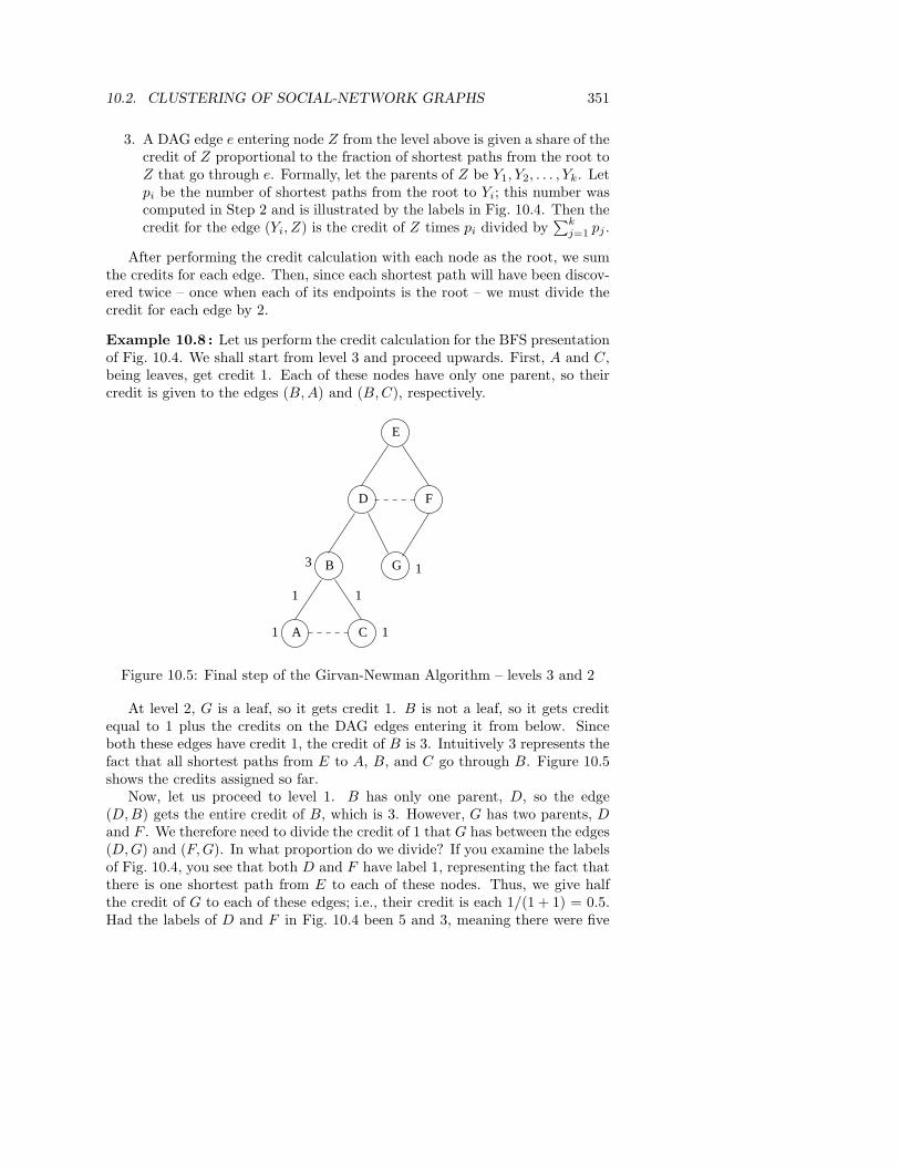
Example 10.8 : Let us perform the credit calculation for the BFS presentationof Fig. 10.4. We shall start from level 3 and proceed upwards. First, A and C,being leaves, get credit 1. Each of these nodes have only one parent, so theircredit is given to the edges (B, A) and (B, C), respectively.

E

D F

B G

A C1 1

3 1

1 1

Figure 10.5: Final step of the Girvan-Newman Algorithm – levels 3 and 2

At level 2, G is a leaf, so it gets credit 1. B is not a leaf, so it gets creditequal to 1 plus the credits on the DAG edges entering it from below. Sinceboth these edges have credit 1, the credit of B is 3. Intuitively 3 represents thefact that all shortest paths from E to A, B, and C go through B. Figure 10.5shows the credits assigned so far.

Now, let us proceed to level 1. B has only one parent, D, so the edge(D, B) gets the entire credit of B, which is 3. However, G has two parents, Dand F . We therefore need to divide the credit of 1 that G has between the edges(D, G) and (F, G). In what proportion do we divide? If you examine the labelsof Fig. 10.4, you see that both D and F have label 1, representing the fact thatthere is one shortest path from E to each of these nodes. Thus, we give halfthe credit of G to each of these edges; i.e., their credit is each 1/(1 + 1) = 0.5.Had the labels of D and F in Fig. 10.4 been 5 and 3, meaning there were five


shortest paths to D and only three to F , then the credit of edge (D, G) wouldhave been 5/8 and the credit of edge (F, G) would have been 3/8.

E

D F

B G

A C1 1

3 1

1 1

0.50.5

4.5 1.5

3

4.5 1.5

Figure 10.6: Final step of the Girvan-Newman Algorithm – completing thecredit calculation

Now, we can assign credits to the nodes at level 1. D gets 1 plus the creditsof the edges entering it from below, which are 3 and 0.5. That is, the credit of Dis 4.5. The credit of F is 1 plus the credit of the edge (F, G), or 1.5. Finally, theedges (E, D) and (E, F ) receive the credit of D and F , respectively, since eachof these nodes has only one parent. These credits are all shown in Fig. 10.6.

The credit on each of the edges in Fig. 10.6 is the contribution to the be-tweenness of that edge due to shortest paths from E. For example, this contri-bution for the edge (E, D) is 4.5. 2

To complete the betweenness calculation, we have to repeat this calculationfor every node as the root and sum the contributions. Finally, we must divideby 2 to get the true betweenness, since every shortest path will be discoveredtwice, once for each of its endpoints.

10.2.5 Using Betweenness to Find Communities

The betweenness scores for the edges of a graph behave something like a distancemeasure on the nodes of the graph. It is not exactly a distance measure, becauseit is not defined for pairs of nodes that are unconnected by an edge, and mightnot satisfy the triangle inequality even when defined. However, we can clusterby taking the edges in order of increasing betweenness and add them to thegraph one at a time. At each step, the connected components of the graphform some clusters. The higher the betweenness we allow, the more edges weget, and the larger the clusters become.

More commonly, this idea is expressed as a process of edge removal. Startwith the graph and all its edges; then remove edges with the highest between-


ness, until the graph has broken into a suitable number of connected compo-nents.

Example 10.9 : Let us start with our running example, the graph of Fig. 10.1.We see it with the betweenness for each edge in Fig. 10.7. The calculation ofthe betweenness will be left to the reader. The only tricky part of the countis to observe that between E and G there are two shortest paths, one goingthrough D and the other through F . Thus, each of the edges (D, E), (E, F ),(D, G), and (G, F ) are credited with half a shortest path.

A B D E

G F

C

5

12

41

5 4.5

1.5

1.5

4.5

Figure 10.7: Betweenness scores for the graph of Fig. 10.1

Clearly, edge (B, D) has the highest betweenness, so it is removed first.That leaves us with exactly the communities we observed make the most sense:A, B, C and D, E, F, G. However, we can continue to remove edges. Nextto leave are (A, B) and (B, C) with a score of 5, followed by (D, E) and (D, G)with a score of 4.5. Then, (D, F ), whose score is 4, would leave the graph. Wesee in Fig. 10.8 the graph that remains.

A B D E

G F

C

Figure 10.8: All the edges with betweenness 4 or more have been removed

The “communities” of Fig. 10.8 look strange. One implication is that A andC are more closely knit to each other than to B. That is, in some sense B is a“traitor” to the community A, B, C because he has a friend D outside thatcommunity. Likewise, D can be seen as a “traitor” to the group D, E, F, G,which is why in Fig. 10.8, only E, F , and G remain connected. 2


Speeding Up the Betweenness Calculation

If we apply the method of Section 10.2.4 to a graph of n nodes and e edges,it takes O(ne) running time to compute the betweenness of each edge.That is, BFS from a single node takes O(e) time, as do the two labelingsteps. We must start from each node, so there are n of the computationsdescribed in Section 10.2.4.

If the graph is large – and even a million nodes is large when thealgorithm takes O(ne) time – we cannot afford to execute it as suggested.However, if we pick a subset of the nodes at random and use these asthe roots of breadth-first searches, we can get an approximation to thebetweenness of each edge that will serve in most applications.


Exercise 10.2.1 : Figure 10.9 is an example of a social-network graph. Usethe Girvan-Newman approach to find the number of shortest paths from eachof the following nodes that pass through each of the edges. (a) A (b) B.

A

B C

D

EG

H

FI

Figure 10.9: Graph for exercises

Exercise 10.2.2 : Using symmetry, the calculations of Exercise 10.2.1 are allyou need to compute the betweenness of each edge. Do the calculation.

Exercise 10.2.3 : Using the betweenness values from Exercise 10.2.2, deter-mine reasonable candidates for the communities in Fig. 10.9 by removing alledges with a betweenness above some threshold.

10.3. DIRECT DISCOVERY OF COMMUNITIES 355

10.3 Direct Discovery of Communities

In the previous section we searched for communities by partitioning all the in-dividuals in a social network. While this approach is relatively efficient, it doeshave several limitations. It is not possible to place an individual in two differentcommunities, and everyone is assigned to a community. In this section, we shallsee a technique for discovering communities directly by looking for subsets ofthe nodes that have a relatively large number of edges among them. Interest-ingly, the technique for doing this search on a large graph involves finding largefrequent itemsets, as was discussed in Chapter 6.

10.3.1 Finding Cliques

Our first thought about how we could find sets of nodes with many edgesbetween them is to start by finding a large clique (a set of nodes with edgesbetween any two of them). However, that task is not easy. Not only is findingmaximal cliques NP-complete, but it is among the hardest of the NP-completeproblems in the sense that even approximating the maximal clique is hard.Further, it is possible to have a set of nodes with almost all edges betweenthem, and yet have only relatively small cliques.

Example 10.10 : Suppose our graph has nodes numbered 1, 2, . . . , n and thereis an edge between two nodes i and j unless i and j have the same remain-der when divided by k. Then the fraction of possible edges that are actuallypresent is approximately (k − 1)/k. There are many cliques of size k, of which1, 2, . . . , k is but one example.

Yet there are no cliques larger than k. To see why, observe that any set ofk + 1 nodes has two that leave the same remainder when divided by k. Thispoint is an application of the “pigeonhole principle.” Since there are only kdifferent remainders possible, we cannot have distinct remainders for each ofk + 1 nodes. Thus, no set of k + 1 nodes can be a clique in this graph. 2

10.3.2 Complete Bipartite Graphs

Recall our discussion of bipartite graphs from Section 8.3. A complete bipartite

graph consists of s nodes on one side and t nodes on the other side, with all stpossible edges between the nodes of one side and the other present. We denotethis graph by Ks,t. You should draw an analogy between complete bipartitegraphs as subgraphs of general bipartite graphs and cliques as subgraphs ofgeneral graphs. In fact, a clique of s nodes is often referred to as a complete

graph and denoted Ks, while a complete bipartite subgraph is sometimes calleda bi-clique.

While as we saw in Example 10.10, it is not possible to guarantee that agraph with many edges necessarily has a large clique, it is possible to guar-antee that a bipartite graph with many edges has a large complete bipartite


subgraph.1 We can regard a complete bipartite subgraph (or a clique if wediscovered a large one) as the nucleus of a community and add to it nodeswith many edges to existing members of the community. If the graph itself isk-partite as discussed in Section 10.1.4, then we can take nodes of two typesand the edges between them to form a bipartite graph. In this bipartite graph,we can search for complete bipartite subgraphs as the nuclei of communities.For instance, in Example 10.2, we could focus on the tag and page nodes of agraph like Fig. 10.2 and try to find communities of tags and Web pages. Such acommunity would consist of related tags and related pages that deserved manyor all of those tags.

However, we can also use complete bipartite subgraphs for community find-ing in ordinary graphs where nodes all have the same type. Divide the nodesinto two equal groups at random. If a community exists, then we would expectabout half its nodes to fall into each group, and we would expect that abouthalf its edges would go between groups. Thus, we still have a reasonable chanceof identifying a large complete bipartite subgraph in the community. To thisnucleus we can add nodes from either of the two groups, if they have edges tomany of the nodes already identified as belonging to the community.

10.3.3 Finding Complete Bipartite Subgraphs

Suppose we are given a large bipartite graph G , and we want to find instancesof Ks,t within it. It is possible to view the problem of finding instances of Ks,t

within G as one of finding frequent itemsets. For this purpose, let the “items”be the nodes on one side of G, which we shall call the left side. We assume thatthe instance of Ks,t we are looking for has t nodes on the left side, and we shallalso assume for efficiency that t ≤ s. The “baskets” correspond to the nodeson the other side of G (the right side). The members of the basket for node vare the nodes of the left side to which v is connected. Finally, let the supportthreshold be s, the number of nodes that the instance of Ks,t has on the rightside.

We can now state the problem of finding instances of Ks,t as that of findingfrequent itemsets F of size t. That is, if a set of t nodes on the left side isfrequent, then they all occur together in at least s baskets. But the basketsare the nodes on the right side. Each basket corresponds to a node that isconnected to all t of the nodes in F . Thus, the frequent itemset of size t and sof the baskets in which all those items appear form an instance of Ks,t.

Example 10.11 : Recall the bipartite graph of Fig. 8.1, which we repeat here asFig. 10.10. The left side is the nodes 1, 2, 3, 4 and the right side is a, b, c, d.The latter are the baskets, so basket a consists of “items” 1 and 4; that is,a = 1, 4. Similarly, b = 2, 3, c = 1 and d = 3.

1It is important to understand that we do not mean a generated subgraph – one formedby selecting some nodes and including all edges. In this context, we only require that therebe edges between any pair of nodes on different sides. It is also possible that some nodes onthe same side are connected by edges as well.

10.3. DIRECT DISCOVERY OF COMMUNITIES 357

4

1 a

b

c

d

2

3

Figure 10.10: The bipartite graph from Fig. 8.1

If s = 2 and t = 1, we must find itemsets of size 1 that appear in at leasttwo baskets. 1 is one such itemset, and 3 is another. However, in this tinyexample there are no itemsets for larger, more interesting values of s and t,such as s = t = 2. 2

10.3.4 Why Complete Bipartite Graphs Must Exist

We must now turn to the matter of demonstrating that any bipartite graphwith a sufficiently high fraction of the edges present will have an instance ofKs,t. In what follows, assume that the graph G has n nodes on the left andanother n nodes on the right. Assume the two sides have the same number ofnodes simplifies the calculation, but the argument generalizes to sides of anysize. Finally, let d be the average degree of all nodes.

The argument involves counting the number of frequent itemsets of size tthat a basket with d items contributes to. When we sum this number over allnodes on the right side, we get the total frequency of all the subsets of size t onthe left. When we divide by

(

nt

)

, we get the average frequency of all itemsetsof size t. At least one must have a frequency that is at least average, so if thisaverage is at least s, we know an instance of Ks,t exists.

Now, we provide the detailed calculation. Suppose the degree of the ithnode on the right is di; that is, di is the size of the ith basket. Then thisbasket contributes to

(

di

t

)

itemsets of size t. The total contribution of the n

nodes on the right is∑

i

(

di

t

)

. The value of this sum depends on the di’s, ofcourse. However, we know that the average value of di is d. It is known thatthis sum is minimized when each di is d. We shall not prove this point, but asimple example will suggest the reasoning: since

(

di

t

)

grows roughly as the tth


power of di, moving 1 from a large di to some smaller dj will reduce the sum

of(

di

t

)

+(

dj

t

)

.

Example 10.12 : Suppose there are only two nodes, t = 2, and the averagedegree of the nodes is 4. Then d1+d2 = 8, and the sum of interest is

(

d1

2

)

+(

d2

2

)

.

If d1 = d2 = 4, then the sum is(

42

)

+(

42

)

= 6 + 6 = 12. However, if d1 = 5 and

d2 = 3, the sum is(

52

)

+(

32

)

= 10 + 3 = 13. If d1 = 6 and d1 = 2, then the sum

is(

62

)

+(

22

)

= 15 + 1 = 16. 2

Thus, in what follows, we shall assume that all nodes have the average degreed. So doing minimizes the total contribution to the counts for the itemsets, andthus makes it least likely that there will be a frequent itemset (itemset withwith support s or more) of size t. Observe the following:

• The total contribution of the n nodes on the right to the counts of theitemsets of size t is n

(

dt

)

.

• The number of itemsets of size t is(

nt

)

.

• Thus, the average count of an itemset of size t is n(

dt

)

/(

nt

)

; this expressionmust be at least s if we are to argue that an instance of Ks,t exists.

If we expand the binomial coefficients in terms of factorials, we find

n

(

d

t

)

/

(

n

t

)

= nd!(n − t)!t!/(

(d − t)!t!n!)

=

n(d)(d − 1) · · · (d − t + 1)/(

n(n − 1) · · · (n − t + 1))

To simplify the formula above, let us assume that n is much larger than d, andd is much larger than t. Then d(d − 1) · · · (d − t + 1) is approximately dt, andn(n − 1) · · · (n − t + 1) is approximately nt. We thus require that

n(d/n)t ≥ s

That is, if there is a community with n nodes on each side, the average degreeof the nodes is d, and n(d/n)t ≥ s, then this community is guaranteed to havea complete bipartite subgraph Ks,t. Moreover, we can find the instance of Ks,t

efficiently, using the methods of Chapter 6, even if this small community isembedded in a much larger graph. That is, we can treat all nodes in the entiregraph as baskets and as items, and run A-priori or one of its improvements onthe entire graph, looking for sets of t items with support s.

Example 10.13 : Suppose there is a community with 100 nodes on each side,and the average degree of nodes is 50; i.e., half the possible edges exist. Thiscommunity will have an instance of Ks,t, provided 100(1/2)t ≥ s. For example,if t = 2, then s can be as large as 25. If t = 3, s can be 11, and if t = 4, s canbe 6.

10.4. PARTITIONING OF GRAPHS 359

Unfortunately, the approximation we made gives us a bound on s that is alittle too high. If we revert to the original formula n

(

dt

)

/(

nt

)

≥ s, we see that

for the case t = 4 we need 100(

504

)

/(

1004

)

≥ s. That is,

100 × 50 × 49 × 48 × 47

100 × 99 × 98 × 97≥ s

The expression on the left is not 6, but only 5.87. However, if the averagesupport for an itemset of size 4 is 5.87, then it is impossible that all thoseitemsets have support 5 or less. Thus, we can be sure that at least one itemsetof size 4 has support 6 or more, and an instance of K6.4 exists in this community.2


Exercise 10.3.1 : For the running example of a social network from Fig. 10.1,how many instances of Ks,t are there for:

(a) s = 1 and t = 3.

(b) s = 2 and t = 2.

(c) s = 2 and t = 3.

Exercise 10.3.2 : Suppose there is a community of 2n nodes. Divide thecommunity into two groups of n members, at random, and form the bipartitegraph between the two groups. Suppose that the average degree of the nodes ofthe bipartite graph is d. Find the set of maximal pairs (t, s), with t ≤ s, suchthat an instance of Ks,t is guaranteed to exist, for the following combinationsof n and d:

(a) n = 20 and d = 5.

(b) n = 200 and d = 150.

(c) n = 1000 and d = 400.

By “maximal,” we mean there is no different pair (s′, t′) such that both s′ ≥ sand t′ ≥ t hold.

10.4 Partitioning of Graphs

In this section, we examine another approach to organizing social-networkgraphs. We use some important tools from matrix theory (“spectral meth-ods”) to formulate the problem of partitioning a graph to minimize the numberof edges that connect different components. The goal of minimizing the “cut”size needs to be understood carefully before proceeding. For instance, if you


just joined Facebook, you are not yet connected to any friends. We do notwant to partition the friends graph with you in one group and the rest of theworld in the other group, even though that would partition the graph withoutthere being any edges that connect members of the two groups. This cut is notdesirable because the two components are too unequal in size.

10.4.1 What Makes a Good Partition?

Given a graph, we would like to divide the nodes into two sets so that the cut, orset of edges that connect nodes in different sets is minimized. However, we alsowant to constrain the selection of the cut so that the two sets are approximatelyequal in size. The next example illustrates the point.

Example 10.14 : Recall our running example of the graph in Fig. 10.1. There,it is evident that the best partition puts A, B, C in one set and D, E, F, Gin the other. The cut consists only of the edge (B, D) and is of size 1. Nonontrivial cut can be smaller.

A B D E

G F

C

H

Smallest Best cut

cut

Figure 10.11: The smallest cut might not be the best cut

In Fig. 10.11 is a variant of our example, where we have added the node Hand two extra edges, (H, C) and (C, G). If all we wanted was to minimize thesize of the cut, then the best choice is to put H in one set and all the othernodes in the other set. But it should be apparent that if we reject partitionswhere one set is too small, then the best we can do is to use the cut consistingof edges (B, D) and (C, G), which partitions the graph into two equal-sized setsA, B, C, H and D, E, F, G. 2

10.4.2 Normalized Cuts

A proper definition of a “good” cut must balance the size of the cut itselfagainst the difference in the sizes of the sets that the cut creates. One choice


that serves well is the “normalized cut.” First, define the volume of a set S ofnodes, denoted Vol(S), to be the number of edges with at least one end in S.

Suppose we partition the nodes of a graph into two disjoint sets S and T .Let Cut(S, T ) be the number of edges that connect a node in S to a node in T .Then the normalized cut value for S and T is

Cut(S, T )

Vol(S)+

Cut(S, T )

Vol(T )

Example 10.15 : Again consider the graph of Fig. 10.11. If we choose S = Hand T = A, B, C, D, E, F, G, then Cut(S, T ) = 1. Vol(S) = 1, because thereis only one edge connected to H . On the other hand, Vol(T ) = 11, because allthe edges have at least one end at a node of T . Thus, the normalized cut forthis partition is 1/1 + 1/11 = 1.09.

Now, consider the preferred cut for this graph consisting of the edges (B, D)and (C, G). Then S = A, B, C, H and T = D, E, F, G. Cut(S, T ) = 2,Vol(S) = 6, and Vol(T ) = 7. The normalized cut for this partition is thus only2/6 + 2/7 = 0.62. 2

10.4.3 Some Matrices That Describe Graphs

To develop the theory of how matrix algebra can help us find good graphpartitions, we first need to learn about three different matrices that describeaspects of a graph. The first should be familiar: the adjacency matrix that hasa 1 in row i and column j if there is an edge between nodes i and j, and 0otherwise.

A B D E

G F

C

Figure 10.12: Repeat of the graph of Fig. 10.1

Example 10.16 : We repeat our running example graph in Fig. 10.12. Itsadjacency matrix appears in Fig. 10.13. Note that the rows and columns cor-respond to the nodes A, B, . . . , G in that order. For example, the edge (B, D)is reflected by the fact that the entry in row 2 and column 4 is 1 and so is theentry in row 4 and column 2. 2

The second matrix we need is the degree matrix for a graph. This graph hasentries only on the diagonal. The entry for row and column i is the degree ofthe ith node.


0 1 1 0 0 0 01 0 1 1 0 0 01 1 0 0 0 0 00 1 0 0 1 1 10 0 0 1 0 1 00 0 0 1 1 0 10 0 0 1 0 1 0

Figure 10.13: The adjacency matrix for Fig. 10.12

Example 10.17 : The degree matrix for the graph of Fig. 10.12 is shown inFig. 10.14. We use the same order of the nodes as in Example 10.16. Forinstance, the entry in row 4 and column 4 is 4 because node D has edges tofour other nodes. The entry in row 4 and column 5 is 0, because that entry isnot on the diagonal. 2

2 0 0 0 0 0 00 3 0 0 0 0 00 0 2 0 0 0 00 0 0 4 0 0 00 0 0 0 2 0 00 0 0 0 0 3 00 0 0 0 0 0 2

Figure 10.14: The degree matrix for Fig. 10.12

Suppose our graph has adjacency matrix A and degree matrix D. Our thirdmatrix, called the Laplacian matrix, is L = D − A, the difference between thedegree matrix and the adjacency matrix. That is, the Laplacian matrix L hasthe same entries as D on the diagonal. Off the diagonal, at row i and column j,L has −1 if there is an edge between nodes i and j and 0 if not.

Example 10.18 : The Laplacian matrix for the graph of Fig. 10.12 is shownin Fig. 10.15. Notice that each row and each column sums to zero, as must bethe case for any Laplacian matrix. 2

10.4.4 Eigenvalues of the Laplacian Matrix

We can get a good idea of the best way to partition a graph from the eigenvaluesand eigenvectors of its Laplacian matrix. In Section 5.1.2 we observed how theprincipal eigenvector (eigenvector associated with the largest eigenvalue) of thetransition matrix of the Web told us something useful about the importance ofWeb pages. In fact, in simple cases (no taxation) the principal eigenvector is the


2 -1 -1 0 0 0 0-1 3 -1 -1 0 0 0-1 -1 2 0 0 0 00 -1 0 4 -1 -1 -10 0 0 -1 2 -1 00 0 0 -1 -1 3 -10 0 0 -1 0 -1 2

Figure 10.15: The Laplacian matrix for Fig. 10.12

PageRank vector. When dealing with the Laplacian matrix, however, it turnsout that the smallest eigenvalues and their eigenvectors reveal the informationwe desire.

The smallest eigenvalue for every Laplacian matrix is 0, and its correspond-ing eigenvector is [1, 1, . . . , 1]. To see why, let L be the Laplacian matrix for agraph of n nodes, and let 1 be the column vector of all 1’s with length n. Weclaim L1 is a column vector of all 0’s. To see why, consider row i of L. Itsdiagonal element has the degree d of node i. Row i also will have d occurrencesof −1, and all other elements of row i are 0. Multiplying row i by column vector1 has the effect of summing the row, and this sum is clearly d + (−1)d = 0.Thus, we can conclude L1 = 01, which demonstrates that 0 is an eigenvalueand 1 its corresponding eigenvector.

There is a simple way to find the second-smallest eigenvalue for any matrix,such as the Laplacian matrix, that is symmetric (the entry in row i and columnj equals the entry in row j and column i). While we shall not prove thisfact, the second-smallest eigenvalue of L is the minimum of xT Lx, where x =[x1, x2, . . . , xn] is a column vector with n components, and the minimum istaken under the constraints:

1. The length of x is 1; that is∑n

i=1 x2i = 1.

2. x is orthogonal to the eigenvector associated with the smallest eigenvalue.

Moreover, the value of x that achieves this minimum is the second eigenvector.When L is a Laplacian matrix for an n-node graph, we know something

more. The eigenvector associated with the smallest eigenvalue is 1. Thus, if x

is orthogonal to 1, we must have

xT 1 =

n∑

i=1

xi = 0

In addition for the Laplacian matrix, the expression xT Lx has a useful equiv-alent expression. Recall that L = D − A, where D and A are the degree andadjacency matrices of the same graph. Thus, xT Lx = xT Dx − xT Ax. Let usevaluate the term with D and then the term for A. Dx is the column vector


[d1x1, d2x2, . . . , dnxn], where di is the degree of the ith node of the graph. Thus,xT Dx is

∑ni=1 dix

2i .

Now, turn to xT Ax. The ith component of the column vector Ax is the sumof xj over all j such that there is an edge (i, j) in the graph. Thus, −xT Ax is thesum of −2xixj over all pairs of nodes i, j such that there is an edge betweenthem. Note that the factor 2 appears because each set i, j corresponds to twoterms, −xixj and −xjxi.

We can group the terms of xT Lx in a way that distributes the terms to eachpair i, j. From −xT Ax, we already have the term −2xixj . From xT Dx, wedistribute the term dix

2i to the di pairs that include node i. As a result, we

can associate with each pair i, j that has an edge between nodes i and j theterms x2

i −2xixj +x2j . This expression is equivalent to (xi−xj)

2. Therefore, we

have proved that xT Lx equals the sum over all graph edges (i, j) of (xi − xj)2.

Recall that the second-smallest eigenvalue is the minimum of this expressionunder the constraint that

∑ni=1 x2

i = 1. Intuitively, we minimize it by makingxi and xj close whenever there is an edge between nodes i and j in the graph.We might imagine that we could choose xi = 1/

√n for all i and thus make this

sum 0. However, recall that we are constrained to choose x to be orthogonal to1, which means the sum of the xi’s is 0. We are also forced to make

∑ni=1 x2

i be1, so all components cannot be 0. As a consequence, x must have some positiveand some negative components.

We can obtain a partition of the graph by taking one set to be the nodesi whose corresponding vector component xi is positive and the other set tobe those whose components are negative. This choice does not guarantee apartition into sets of equal size, but the sizes are likely to be close. We believethat the cut between the two sets will have a small number of edges because(xi−xj)

2 is likely to be smaller if both xi and xj have the same sign than if theyhave different signs. Thus, minimizing xT Lx under the required constraints willtend to give xi and xj the same sign if there is an edge (i, j).

2

3 6

5

41

Figure 10.16: Graph for illustrating partitioning by spectral analysis

Example 10.19 : Let us apply the above technique to the graph of Fig. 10.16.The Laplacian matrix for this graph is shown in Fig. 10.17. By standard meth-ods or math packages we can find all the eigenvalues and eigenvectors of thismatrix. We shall simply tabulate them in Fig. 10.18, from lowest eigenvalue tohighest. Note that we have not scaled the eigenvectors to have length 1, butcould do so easily if we wished.


3 -1 -1 -1 0 0-1 2 -1 0 0 0-1 -1 3 0 0 -1-1 0 0 3 -1 -10 0 0 -1 2 -10 0 -1 -1 -1 3

Figure 10.17: The Laplacian matrix for Fig. 10.16

The second eigenvector has three positive and three negative components.It makes the unsurprising suggestion that one group should be 1, 2, 3, thenodes with positive components, and the other group should be 4, 5, 6. 2

Eigenvalue 0 1 3 3 4 5Eigenvector 1 1 −5 −1 −1 −1

1 2 4 −2 1 01 1 1 3 −1 11 −1 −5 −1 1 11 −2 4 −2 −1 01 −1 1 3 1 −1

Figure 10.18: Eigenvalues and eigenvectors for the matrix of Fig. 10.17

10.4.5 Alternative Partitioning Methods

The method of Section 10.4.4 gives us a good partition of the graph into twopieces that have a small cut between them. There are several ways we can usethe same eigenvectors to suggest other good choices of partition. First, we arenot constrained to put all the nodes with positive components in the eigenvectorinto one group and those with negative components in the other. We could setthe threshold at some point other than zero.

For instance, suppose we modified Example 10.19 so that the threshold wasnot zero, but −1.5. Then the two nodes 4 and 6, with components −1 in thesecond eigenvector of Fig. 10.18, would join 1, 2, and 3, leaving five nodes in onecomponent and only node 6 in the other. That partition would have a cut of sizetwo, as did the choice based on the threshold of zero, but the two componentshave radically different sizes, so we would tend to prefer our original choice.However, there are other cases where the threshold zero gives unequally sizedcomponents, as would be the case if we used the third eigenvector in Fig. 10.18.

We may also want a partition into more than two components. One approachis to use the method described above to split the graph into two, and then useit repeatedly on the components to split them as far as desired. A second


approach is to use several of the eigenvectors, not just the second, to partitionthe graph. If we use m eigenvectors, and set a threshold for each, we can get apartition into 2m groups, each group consisting of the nodes that are above orbelow threshold for each of the eigenvectors, in a particular pattern.

It is worth noting that each eigenvector except the first is the vector x thatminimizes xT Lx, subject to the constraint that it is orthogonal to all previouseigenvectors. This constraint generalizes the constraints we described for thesecond eigenvector in a natural way. As a result, while each eigenvector triesto produce a minimum-sized cut, the fact that successive eigenvectors have tosatisfy more and more constraints generally causes the cuts they describe to beprogressively worse.

Example 10.20 : Let us reconsider the graph of Fig. 10.16, for which theeigenvectors of its Laplacian matrix were tabulated in Fig. 10.18. The thirdeigenvector, with a threshold of 0, puts nodes 1 and 4 in one group and theother four nodes in the other. That is not a bad partition, but its cut size isfour, compared with the cut of size two that we get from the second eigenvector.

If we use both the second and third eigenvectors, we put nodes 2 and 3 inone group, because their components are positive in both eigenvectors. Nodes5 and 6 are in another group, because their components are negative in thesecond eigenvector and positive in the third. Node 1 is in a group by itselfbecause it is positive in the second eigenvector and negative in the third, whilenode 4 is also in a group by itself because its component is negative in botheigenvectors. This partition of a six-node graph into four groups is too fine apartition to be meaningful. But at least the groups of size two each have anedge between the nodes, so it is as good as we could ever get for a partitioninto groups of these sizes. 2


Exercise 10.4.1 : For the graph of Fig. 10.9, construct:

(a) The adjacency matrix.

(b) The degree matrix.

(c) The Laplacian matrix.

! Exercise 10.4.2 : For the Laplacian matrix constructed in Exercise 10.4.1(c),find the second-smallest eigenvalue and its eigenvector. What partition of thenodes does it suggest?

!! Exercise 10.4.3 : For the Laplacian matrix constructed in Exercise 10.4.1(c),construct the third and subsequent smallest eigenvalues and their eigenvectors.

10.5. FINDING OVERLAPPING COMMUNITIES 367

10.5 Finding Overlapping Communities

So far, we have concentrated on clustering a social graph to find communities.But communities are in practice rarely disjoint. In this section, we explain amethod for taking a social graph and fitting a model to it that best explains howit could have been generated by a mechanism that assumes the probability thattwo individuals are connected by an edge (are “friends”) increases as they aremembers of more communities in common. An important tool in this analysisis “maximum-likelihood estimation,” which we shall explain before getting tothe matter of finding overlapping communities.

10.5.1 The Nature of Communities

To begin, let us consider what we would expect two overlapping communitiesto look like. Our data is a social graph, where nodes are people and there is anedge between two nodes if the people are “friends.” Let us imagine that thisgraph represents students at a school, and there are two clubs in this school:the Chess Club and the Spanish Club. It is reasonable to suppose that eachof these clubs forms a community, as does any other club at the school. It isalso reasonable to suppose that two people in the Chess Club are more likely tobe friends in the graph because they know each other from the club. Likewise,if two people are in the Spanish Club, then there is a good chance they knoweach other, and are likely to be friends.

What if two people are in both clubs? They now have two reasons why theymight know each other, and so we would expect an even greater probabilitythat they will be friends in the social graph. Our conclusion is that we expectedges to be dense within any community, but we expect edges to be even denserin the intersection of two communities, denser than that in the intersection ofthree communities, and so on. The idea is suggested by Fig. 10.19.

10.5.2 Maximum-Likelihood Estimation

Before we see the algorithm for finding communities that have overlap of thekind suggested by Section 10.5.1, let us digress and learn a useful modelingtool called maximum-likelihood estimation, or MLE. The idea behind MLEis that we make an assumption about the generative process (the model) thatcreates instances of some artifact, for example, “friends graphs.” The model hasparameters that determine the probability of generating any particular instanceof the artifact; this probability is called the likelihood of those parameter values.We assume that the value of the parameters that gives the largest value of thelikelihood is the correct model for the observed artifact.

An example should make the MLE principle clear. For instance, we mightwish to generate random graphs. We suppose that each edge is present withprobability p and not present with probability 1−p, with the presence or absenceof each edge chosen independently. The only parameter we can adjust is p. For


Chess Club Spanish Club

Intersection

Figure 10.19: The overlap of two communities is denser than the nonoverlappingparts of these communities

each value of p there is a small but nonzero probability that the graph generatedwill be exactly the one we see. Following the MLE principle, we shall declarethat the true value of p is the one for which the probability of generating theobserved graph is the highest.

Example 10.21 : Consider the graph of Fig. 10.19. There are 15 nodes and23 edges. As there are 105 pairs of 15 nodes, we see that if each edge is chosenwith probability p, then the probability (likelihood) of generating exactly thegraph of Fig. 10.19 is given by the function p23(1− p)82. No matter what valuep has between 0 and 1, that is an incredibly tiny number. But the function doeshave a maximum, which we can determine by taking its derivative and settingthat to 0. That is:

23p22(1 − p)82 − 82p23(1 − p)81 = 0

We can group terms to rewrite the above as

p22(1 − p)81(

23(1 − p) − 82p)

= 0

The only way the right side can be 0 is if p is 0 or 1, or the last factor,(

23(1 − p) − 82p)

is 0. When p is 0 or 1, the value of the likelihood function p23(1 − p)82 isminimized, not maximized, so it must be the last factor that is 0. That is, the


Prior Probabilities

When we do an MLE analysis, we generally assume that the parameterscan take any value in their range, and there is no bias in favor of particularvalues. However, if that is not the case, then we can multiply the formulawe get for the probability of the observed artifact being generated, asa function of the parameter values, by the function that represents therelative likelihood of those values of the parameter being the true values.The exercises offer examples of MLE with assumptions about the priordistribution of the parameters.

likelihood of generating the graph of Fig. 10.19 is maximized when

23 − 23p− 82p = 0

or p = 23/105.That outcome is hardly a surprise. It says the most likely value for p is the

observed fraction of possible edges that are present in the graph. However, whenwe use a more complicated mechanism to generate graphs or other artifacts,the value of the parameters that produce the observed artifact with maximumlikelihood is far from obvious. 2

10.5.3 The Affiliation-Graph Model

We shall now introduce a reasonable mechanism, called the affiliation-graph

model, to generate social graphs from communities. Once we see how the pa-rameters of the model influence the likelihood of seeing a given graph, we canaddress how one would solve for the values of the parameters that give themaximum likelihood. The mechanism, called community-affiliation graphs.

1. There is a given number of communities, and there is a given number ofindividuals (nodes of the graph).

2. Each community can have any set of individuals as members. That is,the memberships in the communities are parameters of the model.

3. Each community C has a probability pC associated with it, the probabilitythat two members of community C are connected by an edge because theyare both members of C. These probabilities are also parameters of themodel.

4. If a pair of nodes is in two or more communities, then they have an edgebetween them if any of the communities in which they are joint memberscause them to have an edge.


We must compute the likelihood that a given graph with the proper numberof nodes is generated by this mechanism. The key observation is how the edgeprobabilities are computed, given an assignment of individuals to communitiesand values of the pC ’s. Consider an edge (u, v) between nodes u and v. Supposeu and v are members of communities C and D, but not any other communities.Then the probability that there is no edge between u and v is the product ofthe probabilities that there is no edge due to community C and no edge dueto community D. That is, with probability (1 − pC)(1 − pD) there is no edge(u, v) in the graph, and of course the probability that there is such an edge is1 minus that.

More generally, if u and v are members of a nonempty set of communitiesM and not any others, then puv, the probability of an edge between u and v isgiven by:

puv = 1 −∏

C in M

(1 − pC)

As an important special case, if u and v are not in any communities together,then we take puv to be ǫ, some very tiny number. We have to choose thisprobability to be nonzero, or else we can never assign a nonzero likelihoodto any set of communities that do not have every pair of individuals sharinga community. But by taking the probability to be very small, we bias ourcomputation to favor solutions such that every observed edge is explained byjoint membership in some community.

If we know which nodes are in which communities, then we can computethe likelihood of the given graph for these edge probabilities using a simplegeneralization of Example 10.21. Let Muv be the set of communities to whichboth u and v are assigned. Then the likelihood of E being exactly the set ofedges in the observed graph is

∏

(u,v) in E

puv

∏

(u,v) not in E

(1 − puv)

y z

w

x

Figure 10.20: A social graph

Example 10.22 : Consider the tiny social graph in Fig. 10.20. Suppose thereare two communities C and D, with associated probabilities pC and pD. Also,suppose that we have determined (or are using as a temporary hypothesis) thatC = w, x, y and D = w, y, z. To begin, consider the pair of nodes w and


x. Mwx = C; that is, this pair is in community C but not in community D.Therefore, pwx = 1 − (1 − pC) = pC .

Similarly, x and y are only together in C, y and z are only together in D,and likewise w and z are only together in D. Thus, we find pxy = pC andpyz = pwz = pD. Now the pair w and y are together in both communities, sopwy = 1− (1−pC)(1−pD) = pC +pD−pCpD. Finally, x and z are not togetherin either community, so pxz = ǫ.

Now, we can compute the likelihood of the graph in Fig. 10.20, given ourassumptions about membership in the two communities. This likelihood is theproduct of the probabilities associated with each of the four pairs of nodeswhose edges appear in the graph, times one minus the probability for each ofthe two pairs whose edges are not there. That is, we want

pwxpwypxypyz(1 − pwz)(1 − pxz)

Substituting the expressions we developed above for each of these probabilities,we get

(pC)2pD(pC + pD − pCpD)(1 − pD)(1 − ǫ)

Note that ǫ is very small, so the last factor is essentially 1 and can be dropped.We must find the values of pC and pD that maximize the above expression.

First, notice that all factors are either independent of pC or grow with pC . Theonly hard step in this argument is to remember that pD ≤ 1, so

pC + pD − pCpD

must grow positively with pC . It follows that the likelihood is maximized whenpC is as large as possible; that is, pC = 1.

Next, we must find the value of pD that maximizes the expression, giventhat pC = 1. The expression becomes pD(1 − pD), and it is easy to see thatthis expression has its maximum at pD = 0.5. That is, given C = w, x, y andD = w, y, z, the maximum likelihood for the graph in Fig. 10.20 occurs whenmembers of C are certain to have an edge between them and there is a 50%chance that joint membership in D will cause an edge between the members.2

However, Example 10.22 reflects only part of the solution. We also needto find an assignment of members to communities such that the maximumlikelihood solution for that assignment is the largest solution for any assignment.Once we fix on an assignment, finding the probabilities associated with eachcommunity, the pC ’s, can be accomplished, even for very large graphs with largenumbers of communities. The general method for doing so is called “gradientdescent,” a technique that we introduced in Section 9.4.5 and that will bediscussed further starting in Section 12.3.4.

Unfortunately, it is not obvious how one incorporates the set of members ofeach community into the gradient-descent solution, since changes to the com-position of communities is by discrete steps, not according to some continuous


Log Likelihood

Usually, we compute the logarithm of the likelihood function (the log like-

lihood), rather than the function itself. Doing so offers several advantages.Products become sums, which often simplifies the expression. Also, sum-ming many numbers is less prone to numerical rounding errors than istaking the product of many tiny numbers.

function, as is required for gradient descent. The only feasible way to searchthe space of possible assignments of members to communities is by startingwith an assignment and making small changes, say insertion or deletion of onemember for one community. For each such assignment, we can solve for the bestcommunity probabilities (the pC ’s) by gradient descent. However, figuring outwhat changes to membership lead us in the right direction is tricky, and thereis no guarantee you can even get to the best assignment by making incrementalchanges from a starting assignment.

10.5.4 Avoiding the Use of Discrete Membership Changes

There is a solution to the problem caused by the mechanism of Section 10.5.3,where membership of individuals in communities is discrete; either you are amember of the community or not. We can think of “strength of membership”of individuals in communities. Intuitively, the stronger the membership of twoindividuals in the same community, the more likely it is that this communitywill cause them to have an edge between them. In this model, we can adjustthe strength of membership for an individual in a community continuously, justas we can adjust the probability associated with a community in the affiliation-graph model. That improvement allows us to use standard methods, such asgradient descent, to maximize the expression for likelihood. In the improvedmodel, we have

1. Fixed sets of communities and individuals, as before.

2. For each community C and individual x, there is a strength of membership

parameter FxC . These parameters can take any nonnegative value, and avalue of 0 means the individual is definitely not in the community.

3. The probability that community C causes there to be an edge betweennodes u and v is

pC(u, v) = 1 − e−FuCFvC

As before the probability of there being an edge between u and v is 1 minusthe probability that none of the communities causes there to be an edge betweenthem. That is, each community independently causes edges, and an edge exists


between two nodes if any community causes it to exist. More formally, puv, theprobability of an edge between nodes u and v can be calculated as

puv = 1 −∏

C

(

1 − pC(u, v))

If we substitute the formula for pC(u, v) that is assumed in the model, we get

puv = 1 − e−P

CFuCFvC

Finally, let E be the set of edges in the observed graph. As before, we canwrite the formula for the likelihood of the observed graph as the product of theexpression for puv for each edge (u, v) that is in E, times the product of 1−puv

for each edge (u, v) that is not in E. Thus, in the new model, the formula forthe likelihood of the graph with edges E is

∏

(u,v) in E

(1 − e−P

CFuCFvC )

∏

(u,v) not in E

e−P

CFuCFvC

We can simplify this expression somewhat by taking its logarithm. Remem-ber that maximizing a function also maximizes the logarithm of that function,and vice-versa. So we can take the natural logarithm of the above expressionto replace the products by sums. We also get simplification from the fact thatlog(ex) = x.

∑

(u,v) in E

log(1 − e−P

CFuCFvC ) −

∑

(u,v) not in E

∑

C

FuCFvC (10.1)

We can now find the values for the FxC ’s that maximizes the expression(10.1). One way is to use gradient descent in a manner similar to what wasdone in Section 9.4.5. That is, we pick one node x, and adjust all the valuesof the FxC ’s in the direction that most improves the value of (10.1). Noticethat the only factors whose values change in response to changes to the FxC ’sis those where one of u and v is x and the other of u and v is a node adjacent tox. Since the degree of a node is typically much less than the number of edgesin the graph, we can avoid looking at most of the terms in (10.1) at each step.


Exercise 10.5.1 : Suppose graphs are generated by picking a probability p andchoosing each edge independently with probability p, as in Example 10.21. Forthe graph of Fig. 10.20, what value of p gives the maximum likelihood of seeingthat graph? What is the probability this graph is generated?

Exercise 10.5.2 : Compute the MLE for the graph in Example 10.22 for thefollowing guesses of the memberships of the two communities.


(a) C = w, x; C = y, z.

(b) C = w, x, y, z; C = x, y, z.

Exercise 10.5.3 : Suppose we have a coin, which may not be a fair coin, andwe flip it some number of times, seeing h heads and t tails.

(a) If the probability p of getting a head on any flip is p, what is the MLEfor p, in terms of h and t?

(! (b) Suppose we are told that there is a 90% probability that the coin is fair(i.e., p = 0.5), and a 10% chance that p = 0.1. For what values of h andt is it more likely that the coin is fair?

!! (c) Suppose the a-priori likelihood that p has a particular value is proportionalto |p − 0.5|. That is, p is more likely to be near 0 or 1, than around 1/2.If we see h heads and t tails, what is the maximum likelihood estimate ofp?

10.6 Simrank

In this section, we shall take up another approach to analyzing social-networkgraphs. This technique, called “simrank,” applies best to graphs with severaltypes of nodes, although it can in principle be applied to any graph. Thepurpose of simrank is to measure the similarity between nodes of the sametype, and it does so by seeing where random walkers on the graph wind upwhen started at a particular node. Because calculation must be carried outonce for each starting node, it is limited in the sizes of graphs that can beanalyzed completely in this manner.

10.6.1 Random Walkers on a Social Graph

Recall our view of PageRank in Section 5.1 as reflecting what a “random surfer”would do if they walked on the Web graph. We can similarly think of a per-son “walking” on a social network. The graph of a social network is generallyundirected, while the Web graph is directed. However, the difference is unim-portant. A walker at a node N of an undirected graph will move with equalprobability to any of the neighbors of N (those nodes with which N shares anedge).

Suppose, for example, that such a walker starts out at node T1 of Fig. 10.2,which we reproduce here as Fig. 10.21. At the first step, it would go either toU1 or W1. If to W1, then it would next either come back to T1 or go to T2. Ifthe walker first moved to U1, it would wind up at either T1, T2, or T3 next.

We conclude that, starting at T1, there is a good chance the walker wouldvisit T2, at least initially, and that chance is better than the chance it wouldvisit T3 or T4. It would be interesting if we could make the inference that tags

10.6. SIMRANK 375

U

U

T

T

T

T

W

W

W

1

1 1

2

2 2

3 3

4

Figure 10.21: Repeat of Fig. 10.2

T1 and T2 are therefore related or similar in some way. The evidence is thatthey have both been placed on a common Web page, W1, and they have alsobeen used by a common tagger, U1.

However, if we allow the walker to continue traversing the graph at random,then the probability that the walker will be at any particular node does notdepend on where it starts out. This conclusion comes from the theory of Markovprocesses that we mentioned in Section 5.1.2, although the independence fromthe starting point requires additional conditions besides connectedness that thegraph of Fig. 10.21 does satisfy.

10.6.2 Random Walks with Restart

We see from the observations above that it is not possible to measure similar-ity to a particular node by looking at the limiting distribution of the walker.However, we have already seen, in Section 5.1.5, the introduction of a smallprobability that the walker will stop walking at random. Then, we saw in Sec-tion 5.3.2 that there were reasons to select only a subset of Web pages as theteleport set, the pages that the walker would go to when they stopped surfingthe Web at random.

Here, we take this idea to the extreme. As we are focused on one particularnode N of a social network, and want to see where the random walker winds upon short walks from that node, we modify the matrix of transition probabilitiesto have a small additional probability of transitioning to N from any node.Formally, let M be the transition matrix of the graph G. That is, the entry inrow i and column j of M is 1/k if node j of G has degree k, and one of theadjacent nodes is i. Otherwise, this entry is 0. We shall discuss teleporting ina moment, but first, let us look at a simple example of a transition matrix.


Example 10.23 : Figure 10.22 is an example of a very simple network involvingthree pictures, and two tags, “Sky” and “Tree” that have been placed on someof them. Pictures 1 and 3 have both tags, while Picture 2 has only the tag“Sky.” Intuitively, we expect that Picture 3 is more similar to Picture 1 thanPicture 2 is, and an analysis using a random walker with restart at Picture 1will support that intuition.

Picture 1 Picture 2 Picture 3

TreeSky

Figure 10.22: A simple bipartite social graph

We shall use, as an order of the nodes Picture 1, Picture 2, Picture 3, Sky,Tree. Then the transition matrix for the graph of Fig. 10.22 is

0 0 0 1/3 1/20 0 0 1/3 00 0 0 1/3 1/2

1/2 1 1/2 0 01/2 0 1/2 0 0

For example, the fourth column corresponds to the node “Sky,” and this nodeconnects to each of the tree picture nodes. It therefore has degree three, so thenonzero entries in its column must be 1/3. The picture nodes correspond to thefirst three rows and columns, so the entry 1/3 appears in the first three rowsof column 4. Since the “Sky” node does not have an edge to either itself or the“Tree” node, the entries in the last two rows of column 4 are 0. 2

As before, let us use β as the probability that the walker continues at ran-dom, so 1 − β is the probability the walker will teleport to the initial node N .Let eN be the column vector that has 1 in the row for node N and 0’s elsewhere.Then if v is the column vector that reflects the probability the walker is at eachof the nodes at a particular round, and v′ is the probability the walker is ateach of the nodes at the next round, then v′ is related to v by:

v′ = βMv + (1 − β)eN

Example 10.24 : Assume M is the matrix of Example 10.23 and β = 0.8.Also, assume that node N is for Picture 1; that is, we want to compute thesimilarity of other pictures to Picture 1. Then the equation for the new value

10.6. SIMRANK 377

v′ of the distribution that we must iterate is

v′ =

0 0 0 4/15 2/50 0 0 4/15 00 0 0 4/15 2/5

2/5 4/5 2/5 0 02/5 0 2/5 0 0

v +

1/50000

Since the graph of Fig. 10.22 is connected, the original matrix M is stochas-tic, and we can deduce that if the initial vector v has components that sum to1, then v′ will also have components that sum to 1. As a result, we can simplifythe above equation by adding 1/5 to each of the entries in the first row of thematrix. That is, we can iterate the matrix-vector multiplication

v′ =

1/5 1/5 1/5 7/15 3/50 0 0 4/15 00 0 0 4/15 2/5

2/5 4/5 2/5 0 02/5 0 2/5 0 0

v

If we start with v = eN , then the sequence of estimates of the distribution ofthe walker that we get is

10000

1/500

2/52/5

35/758/75

20/756/756/75

95/3758/375

20/375142/375110/375

2353/5625568/5625

1228/5625786/5625690/5625

· · ·

.345

.066

.145

.249

.196

We observe from the above that in the limit, the walker is more than twice aslikely to be at Picture 3 than at Picture 2. This analysis confirms the intuitionthat Picture 3 is more like Picture 1 than Picture 2 is. 2

There are several additional observations that we may take away from Ex-ample 10.24. First, remember that this analysis applies only to Picture 1. If wewanted to know what pictures were most similar to another picture, we wouldhave to start the analysis over for that picture. Likewise, if we wanted to knowabout which tags were most closely associated with the tag “Sky” (an uninter-esting question in this small example, since there is only one other tag), thenwe would have to arrange to have the walker teleport only to the “Sky” node.

Second, notice that convergence takes time, since there is an initial oscil-lation. That is, initially, all the weight is at the pictures, and at the secondstep most of the weight is at the tags. At the third step, most weight is backat the pictures, but at the fourth step much of the weight moves to the tagsagain. However, in the limit there is convergence, with 5/9 of the weight at thepictures and 4/9 of the weight at the tags. In general, the process convergesfor any connected k-partite graph.



Exercise 10.6.1 : If, in Fig. 10.22 you start the walk from Picture 2, what willbe the similarity to Picture 2 of the other two pictures? Which do you expectto be more similar to Picture 2?

Exercise 10.6.2 : If, in Fig. 10.22 you start the walk from Picture 3, what doyou expect the similarity to the other two pictures to be?

! Exercise 10.6.3 : Repeat the analysis of Example 10.24, and compute thesimilarities of Picture 1 to the other pictures, if the following modifications aremade to Fig. 10.22:

(a) The tag “Tree” is added to Picture 2.

(b) A third tag “Water” is added to Picture 3.

(c) A third tag “Water” is added to both Picture 1 and Picture 2.

Note: the changes are independently done for each part; they are not cumula-tive.

10.7 Counting Triangles

One of the most useful properties of social-network graphs is the count of tri-angles and other simple subgraphs. In this section we shall give methods forestimating or getting an exact count of triangles in a very large graph. We be-gin with a motivation for such counting and then give some methods for doingso efficiently.

10.7.1 Why Count Triangles?

If we start with n nodes and add m edges to a graph at random, there will bean expected number of triangles in the graph. We can calculate this numberwithout too much difficulty. There are

(

n3

)

sets of three nodes, or approximatelyn3/6 sets of three nodes that might be a triangle. The probability of an edgebetween any two given nodes being added is m/

(

n2

)

, or approximately 2m/n2.The probability that any set of three nodes has edges between each pair, ifthose edges are independently chosen to be present or absent is approximately(2m/n2)3 = 8m3/n6. Thus, the expected number of triangles in a graph ofn nodes and m randomly selected edges is approximately (8m3/n6)(n3/6) =43 (m/n)3.

If a graph is a social network with n participants and m pairs of “friends,”we would expect the number of triangles to be much greater than the value fora random graph. The reason is that if A and B are friends, and A is also afriend of C, there should be a much greater chance than average that B and

10.7. COUNTING TRIANGLES 379

C are also friends. Thus, counting the number of triangles helps us to measurethe extent to which a graph looks like a social network.

We can also look at communities within a social network. It has beendemonstrated that the age of a community is related to the density of triangles.That is, when a group has just formed, people pull in their like-minded friends,but the number of triangles is relatively small. If A brings in friends B andC, it may well be that B and C do not know each other. As the communitymatures, B and C may interact because of their membership in the community.Thus, there is a good chance that at sometime the triangle A, B, C will becompleted.

10.7.2 An Algorithm for Finding Triangles

We shall begin our study with an algorithm that has the fastest possible runningtime on a single processor. Suppose we have a graph of n nodes and m ≥ nedges. For convenience, assume the nodes are integers 1, 2, . . . , n.

Call a node a heavy hitter if its degree is at least√

m. A heavy-hitter

triangle is a triangle all three of whose nodes are heavy hitters. We use separatealgorithms to count the heavy-hitter triangles and all other triangles. Note thatthe number of heavy-hitter nodes is no more than 2

√m, since otherwise the sum

of the degrees of the heavy hitter nodes would be more than 2m. Since eachedge contributes to the degree of only two nodes, there would then have to bemore than m edges.

Assuming the graph is represented by its edges, we preprocess the graph asfollows:

1. Compute the degree of each node. This part requires only that we examineeach edge and add 1 to the count of each of its two nodes. The total timerequired is O(m).

2. Create an index on edges, with the pair of nodes at its ends as the key.That is, the index allows us to determine, given two nodes, whether theedge between them exists. A hash table suffices. It can be constructed inO(m) time, and the expected time to answer a query about the existenceof an edge is a constant, at least in the expected sense.2

3. Create another index of edges, this one with key equal to a single node.Given a node v, we can retrieve the nodes adjacent to v in time propor-tional to the number of those nodes. Again, a hash table, this time withsingle nodes as the key, suffices in the expected sense.

2Thus, technically, our algorithm is only optimal in the sense of expected running time,not worst-case running time. However, hashing of large numbers of items has an extremelyhigh probability of behaving according to expectation, and if we happened to choose a hashfunction that made some buckets too big, we could rehash until we found a good hash function.


We shall order the nodes as follows. First, order nodes by degree. Then, ifv and u have the same degree, recall that both v and u are integers, so orderthem numerically. That is, we say v ≺ u if and only if either

(i) The degree of v is less than the degree of u, or

(ii) The degrees of u and v are the same, and v < u.

Heavy-Hitter Triangles : There are only O(√

m) heavy-hitter nodes, so wecan consider all sets of three of these nodes. There are O(m3/2) possible heavy-hitter triangles, and using the index on edges we can check if all three edges existin O(1) time. Therefore, O(m3/2) time is needed to find all the heavy-hittertriangles.

Other Triangles: We find the other triangles a different way. Consider eachedge (v1, v2). If both v1 and v2 are heavy hitters, ignore this edge. Suppose,however, that v1 is not a heavy hitter and moreover v1 ≺ v2. Let u1, u2, . . . , uk

be the nodes adjacent to v1. Note that k <√

m. We can find these nodes,using the index on nodes, in O(k) time, which is surely O(

√m) time. For each

ui we can use the first index to check whether edge (ui, v2) exists in O(1) time.We can also determine the degree of ui in O(1) time, because we have countedall the nodes’ degrees. We count the triangle v1, v2, ui if and only if the edge(ui, v2) exists, and v1 ≺ ui. In that way, a triangle is counted only once – whenv1 is the node of the triangle that precedes both other nodes of the triangleaccording to the ≺ ordering. Thus, the time to process all the nodes adjacentto v1 is O(

√m). Since there are m edges, the total time spent counting other

triangles is O(m3/2).

We now see that preprocessing takes O(m) time. The time to find heavy-hitter triangles is O(m3/2), and so is the time to find the other triangles. Thus,the total time of the algorithm is O(m3/2).

10.7.3 Optimality of the Triangle-Finding Algorithm

It turns out that the algorithm described in Section 10.7.2 is, to within anorder of magnitude the best possible. To see why, consider a complete graphon n nodes. This graph has m =

(

n2

)

edges and the number of triangles is(

n3

)

. Since we cannot enumerate triangles in less time than the number of thosetriangles, we know any algorithm will take Ω(n3) time on this graph. However,m = O(n2), so any algorithm takes Ω(m3/2) time on this graph.

One might wonder if there were a better algorithm that worked on sparsergraphs than the complete graph. However, we can add to the complete grapha chain of nodes with any length up to n2. This chain adds no more triangles.It no more than doubles the number of edges, but makes the number of nodesas large as we like, in effect lowering the ratio of edges to nodes to be as closeto 1 as we like. Since there are still Ω(m3/2) triangles, we see that this lowerbound holds for the full range of possible ratios of m/n.


10.7.4 Finding Triangles Using MapReduce

For a very large graph, we want to use parallelism to speed the computation.We can express triangle-finding as a multiway join and use the technique ofSection 2.5.3 to optimize the use of a single MapReduce job to count triangles.It turns out that this use is one where the multiway join technique of that sectionis generally much more efficient than taking two two-way joins. Moreover, thetotal execution time of the parallel algorithm is essentially the same as theexecution time on a single processor using the algorithm of Section 10.7.2.

To begin, assume that the nodes of a graph are numbered 1, 2, . . . , n. Weuse a relation E to represent edges. To avoid representing each edge twice,we assume that if E(A, B) is a tuple of this relation, then not only is therean edge between nodes A and B, but also, as integers, we have A < B.3

This requirement also eliminates loops (edges from a node to itself), which wegenerally assume do not exist in social-network graphs anyway, but which couldlead to “triangles” that really do not involve three different nodes.

Using this relation, we can express the set of triangles of the graph whoseedges are E by the natural join

E(X, Y ) ⊲⊳ E(X, Z) ⊲⊳ E(Y, Z) (10.2)

To understand this join, we have to recognize that the attributes of the relationE are given different names in each of the three uses of E. That is, we imaginethere are three copies of E, each with the same tuples, but with a differentschemas. In SQL, this join would be written using a single relation E(A, B) asfollows:

SELECT e1.A, e1.B, e2.B

FROM E e1, E e2, E e3

WHERE e1.A = e2.A AND e1.B = e3.A AND e2.B = e3.B

In this query, the equated attributes e1.A and e2.A are represented in our joinby the attribute X . Also, e1.B and e3.A are each represented by Y ; e2.B ande3.B are represented by Z.

Notice that each triangle appears once in this join. The triangle consistingof nodes v1, v2, and v3 is generated when X , Y , and Z are these three nodes innumerical order, i.e., X < Y < Z. For instance, if the numerical order of thenodes is v1 < v2 < v3, then X can only be v1, Y is v2, and Z is v3.

The technique of Section 2.5.3 can be used to optimize the join of Equa-tion 10.2. Recall the ideas in Example 2.9, where we considered the numberof ways in which the values of each attribute should be hashed. In the presentexample, the matter is quite simple. The three occurrences of relation E surelyhave the same size, so by symmetry, attributes X , Y , and Z will each be hashed

3Do not confuse this simple numerical ordering of the nodes with the order ≺ that wediscussed in Section 10.7.2 and which involved the degrees of the nodes. Here, node degreesare not computed and are not relevant.


to the same number of buckets. In particular, if we hash nodes to b buckets,then there will be b3 reducers. Each Reduce task is associated with a sequenceof three bucket numbers (x, y, z), where each of x, y, and z is in the range 1 tob.

The Map tasks divide the relation E into as many parts as there are Maptasks. Suppose one Map task is given the tuple E(u, v) to send to certainReduce tasks. First, think of (u, v) as a tuple of the join term E(X, Y ). Wecan hash u and v to get the bucket numbers for X and Y , but we don’t knowthe bucket to which Z hashes. Thus, we must send E(u, v) to all Reducer tasksthat correspond to a sequence of three bucket numbers

(

h(u), h(v), z)

for anyof the b possible buckets z.

But the same tuple E(u, v) must also be treated as a tuple for the termE(X, Z). We therefore also send the tuple E(u, v) to all Reduce tasks thatcorrespond to a triple

(

h(u), y, h(v))

for any y. Finally, we treat E(u, v) as atuple of the term E(Y, Z) and send that tuple to all Reduce tasks correspondingto a triple

(

x, h(u), h(v))

for any x. The total communication required is thus3b key-value pairs for each of the m tuples of the edge relation E. That is, theminimum communication cost is O(mb) if we use b3 Reduce tasks.

Next, let us compute the total execution cost at all the Reduce tasks. As-sume that the hash function distributes edges sufficiently randomly that theReduce tasks each get approximately the same number of edges. Since the totalnumber of edges distributed to the b3 Reduce tasks is O(mb), it follows that eachtask receives O(m/b2) edges. If we use the algorithm of Section 10.7.2 at eachReduce task, the total computation at a task is O

(

(m/b2)3/2)

, or O(m3/2/b3).

Since there are b3 Reduce tasks, the total computation cost is O(m3/2), exactlyas for the one-processor algorithm of Section 10.7.2.

10.7.5 Using Fewer Reduce Tasks

By a judicious ordering of the nodes, we can lower the number of reduce tasksby approximately a factor of 6. Think of the “name” of the node i as thepair

(

h(i), i)

, where h is the hash function that we used in Section 10.7.4 tohash nodes to b buckets. Order nodes by their name, considering only thefirst component (i.e., the bucket to which the node hashes), and only using thesecond component to break ties among nodes that are in the same bucket.

If we use this ordering of nodes, then the Reduce task corresponding tolist of buckets (i, j, k) will be needed only if i ≤ j ≤ k. If b is large, thenapproximately 1/6 of all b3 sequences of integers, each in the range 1 to b, willsatisfy these inequalities. For any b, the number of such sequences is

(

b+23

)

(seeExercise 10.7.4). Thus, the exact ratio is (b + 2)(b + 1)/(6b2).

As there are fewer reducers, we get a substantial decrease in the numberof key-value pairs that must be communicated. Instead of having to send eachof the m edges to 3b Reduce tasks, we need to send each edge to only b tasks.Specifically, consider an edge e whose two nodes hash to i and j; these bucketscould be the same or different. For each of the b values of k between 1 and b,


consider the list formed from i, j, and k in sorted order. Then the Reduce taskthat corresponds to this list requires the edge e. But no other Reduce tasksrequire e.

To compare the communication cost of the method of this section with thatof Section 10.7.4, let us fix the number of Reduce tasks, say k. Then the methodof Section 10.7.4 hashes nodes to 3

√k buckets, and therefore communicates

3m 3√

k key-value pairs. On the other hand, the method of this section hashesnodes to approximately 3

√6k buckets, thus requiring m 3

√6 3√

k communication.Thus, the ratio of the communication needed by the method of Section 10.7.4to what is needed here is 3/ 3

√6 = 1.65.

Example 10.25 : Consider the straightforward algorithm of Section 10.7.4with b = 6. That is, there are b3 = 216 Reduce tasks and the communicationcost is 3mb = 18m. We cannot use exactly 216 Reduce tasks with the method ofthis section, but we can come very close if we choose b = 10. Then, the numberof Reduce tasks is

(

123

)

= 220, and the communication cost is mb = 10m. Thatis, the communication cost is 5/9th of the cost of the straightforward method.2


Exercise 10.7.1 : How many triangles are there in the graphs:

(a) Figure 10.1.

(b) Figure 10.9.

! (c) Figure 10.2.

Exercise 10.7.2 : For each of the graphs of Exercise 10.7.1 determine:

(i) What is the minimum degree for a node to be considered a “heavy hitter”?

(ii) Which nodes are heavy hitters?

(iii) Which triangles are heavy-hitter triangles?

! Exercise 10.7.3 : In this exercise we consider the problem of finding squaresin a graph. That is, we want to find quadruples of nodes a, b, c, d such that thefour edges (a, b), (b, c), (c, d), and (a, d) exist in the graph. Assume the graphis represented by a relation E as in Section 10.7.4. It is not possible to write asingle join of four copies of E that expresses all possible squares in the graph,but we can write three such joins. Moreover, in some cases, we need to followthe join by a selection that eliminates “squares” where one pair of oppositecorners are really the same node. We can assume that node a is numericallylower than its neighbors b and d, but there are three cases,depending on whetherc is


(i) Also lower than b and d,

(ii) Between b and d, or

(iii) Higher than both b and d.

(a) Write the natural joins that produce squares satisfying each of the threeconditions above. You can use four different attributes W , X , Y , and Z,and assume that there are four copies of relation E with different schemas,so the joins can each be expressed as natural joins.

(b) For which of these joins do we need a selection to assure that oppositecorners are really different nodes?

!! (c) Assume we plan to use k Reduce tasks. For each of your joins from (a),into how many buckets should you hash each of W , X , Y , and Z in orderto minimize the communication cost?

(d) Unlike the case of triangles, it is not guaranteed that each square is pro-duced only once, although we can be sure that each square is producedby only one of the three joins. For example, a square in which the twonodes at opposite corners are each lower numerically than the each of theother two nodes will only be produced by the join (i). For each of thethree joins, how many times does it produce each square that it producesat all?

! Exercise 10.7.4 : Show that the number of sequences of integers 1 ≤ i ≤ j ≤k ≤ b is

(

b+23

)

. Hint : show that these sequences can be placed in a 1-to-1correspondence with the binary strings of length b+ 2 having exactly three 1’s.

10.8 Neighborhood Properties of Graphs

There are several important properties of graphs that relate to the number ofnodes one can reach from a given node along a short path. In this sectionwe look at algorithms for solving problems about paths and neighborhoods forvery large graphs. In some cases, exact solutions are not feasible for graphswith millions of nodes. We therefore look at approximation algorithms as wellas exact algorithms.

10.8.1 Directed Graphs and Neighborhoods

In this section we shall use a directed graph as a model of a network. A directed

graph has a set of nodes and a set of arcs ; the latter is a pair of nodes writtenu → v. We call u the source and v the target of the arc. The arc is said to befrom u to v.

Many kinds of graphs can be modeled by directed graphs. The Web is amajor example, where the arc u → v is a link from page u to page v. Or, the

10.8. NEIGHBORHOOD PROPERTIES OF GRAPHS 385

arc u → v could mean that telephone subscriber u has called subscriber v inthe past month. For another example, the arc could mean that individual u isfollowing individual v on Twitter. In yet another graph, the arc could meanthat research paper u references paper v.

Moreover, all undirected graphs can be represented by directed graphs. In-stead of the undirected edge (u, v), use two arcs u → v and v → u. Thus, thematerial of this section also applies to graphs that are inherently undirected,such as a friends graph in a social network.

A path in a directed graph is a sequence of nodes v0, v1, . . . , vk such thatthere are arcs v1 → vi+1 for all i = 0, 1, . . . , k − 1. The length of this path is k,the number of arcs along the path. Note that there are k + 1 nodes in a pathof length k, and a node by itself is considered a path of length 0.

The neighborhood of radius d for a node v is the set of nodes u for whichthere is a path of length at most d from v to u. We denote this neighborhoodby N(v, d). For example, N(v, 0) is always v, and N(v, 1) is v plus the set ofnodes to which there is an arc from v. More generally, if V is a set of nodes,then N(V, d) is the set of nodes u for which there is a path of length d or lessfrom at least one node in the set V .

The neighborhood profile of a node v is the sequence of sizes of its neighbor-hoods |N(v, 1)|, |N(v, 2)|, . . . . We do not include the neighborhood of distance0, since its size is always 1.

A B D E

G F

C

Figure 10.23: Our small social network; think of it as a directed graph

Example 10.26 : Consider the undirected graph of Fig. 10.1, which we repro-duce here as Fig. 10.23. To turn it into a directed graph, think of each edgeas a pair of arcs, one in each direction. For instance, the edge (A, B) becomesthe arcs A → B and B → A. First, consider the neighborhoods of node A.We know N(A, 0) = A. N(A, 1) = A, B, C, since there are arcs from Aonly to B and C. N(A, 2) = A, B, C, D and N(A, 3) = A, B, C, D, E, F, G.Neighborhoods for larger radius are all the same as N(A, 3).

On the other hand, consider node B. We find N(B, 0) = B, N(B, 1) =A, B, C, D, and N(B, 2) = A, B, C, D, E, F, G. We know that B is morecentral to the network than A, and this fact is reflected by the neighborhoodprofiles of the two nodes. Node A has profile 3, 4, 7, 7, . . ., while B has profile4, 7, 7, . . . . Evidently, B is more central than A, because at every distance, its


neighborhood is at least as large as that of A. In fact, D is even more centralthan B, because its neighborhood profile 5, 7, 7, . . . dominates the profile of eachof the nodes. 2

10.8.2 The Diameter of a Graph

The diameter of a directed graph is the smallest integer d such that for everytwo nodes u and v there is a path of length d or less from u to v. In a directedgraph, this definition only makes sense if the graph is strongly connected ; thatis, there is a path from any node to any other node. Recall our discussionof the Web in Section 5.1.3, where we observed that there is a large stronglyconnected subset of the Web in the “center,” but that the Web as a whole isnot strongly connected. Rather, there are some pages that reach nowhere bylinks, and some pages that cannot be reached by links.

If the graph is undirected, the definition of diameter is the same as fordirected graphs, but the path may traverse the undirected edges in either di-rection. That is, we treat an undirected edge as a pair of arcs, one in eachdirection. The notion of diameter makes sense in an undirected graph as longas that graph is connected.

Example 10.27 : For the graph of Fig. 10.23, the diameter is 3. There aresome pairs of nodes, such as A and E, that have no path of length less than3. But every pair of nodes have a path from one to the other with length atmost 3. 2

We can compute the diameter of a graph by computing the sizes of itsneighborhoods of increasing radius, until at some radius we fail to add anymore nodes. That is, for each node v, find the smallest d such that |N(v, d)| =|N(v, d + 1)|. This d is the tight upper bound on the length of the shortestpath from v to any node it can reach. Call it d(v). For instance, we saw fromExample 10.26 that d(A) = 3 and d(B) = 2. If there is any node v such that|N

(

v, d(v))

| is not the number of nodes in the entire graph, then the graph isnot strongly connected, and we cannot offer any finite integer as its diameter.However, if the graph is strongly connected, then the diameter of the graph ismaxv

(

d(v))

.

The reason this computation works is that one way to express N(v, d+1) isthe union of N(v, d) and the set of all nodes w such that for some u in N(v, d)there is an arc u → w. That is, we start with N(v, d) and add to it the targetsof all arcs that have a source in N(v, d). If all the arcs with source in N(v, d)are already in N(v, d), then not only is N(v, d + 1) equal to N(v, d), but all ofN(v, d + 2), N(v, d + 3), . . . will equal N(v, d). Finally, we observe that sinceN(v, d) ⊆ N(v, d+1) the only way |N(v, d)| can equal |N(v, d+1)| is for N(v, d)and N(v, d + 1) to be the same set. Thus, if d is the smallest integer such that|N(v, d)| = |N(v, d + 1)|, it follows that every node v can reach is reached by apath of length at most d.


Six Degrees of Separation

There is a famous game called “six degrees of Kevin Bacon,” the objectof which is to find paths of length at most six in the graph whose nodesare movie stars and whose edges connect stars that played in the samemovie. The conjecture is that in this graph, no movie star is of distancemore than six from Kevin Bacon. More generally, any two movie starscan be connected by a path of length at most six; i.e., the diameter ofthe graph is six. A small diameter makes computation of neighborhoodsmore efficient, so it would be nice if all social-network graphs exhibiteda similar small diameter. In fact, the phrase “six degrees of separation,”refers to the conjecture that in the network of all people in the world,where an edge means that the two people know each other, the diameter issix. Unfortunately, as we shall discuss in Section 10.8.3, not all importantgraphs exhibit such tight connections.

10.8.3 Transitive Closure and Reachability

The transitive closure of a graph is the set of pairs of nodes (u, v) such thatthere is a path from u to v of length zero or more. We shall sometimes writethis assertion as path(u, v).4 A related concept is that of reachability. We saynode u reaches node v if path(u, v). The problem of computing the transitiveclosure is to find all pairs of nodes u and v in a graph for which path(u, v) istrue. The reachability problem is, given a node u in the graph, find all v suchthat path(u, v) is true.

These two concepts relate to the notions of neighborhoods that we haveseen earlier. In fact, path(u, v) is true if and only if v is in N(u,∞), whichwe define to be ∪i≥0 N(u, i). Thus, the reachability problem is to computethe union of all the neighborhoods of any radius for a given node u. Thediscussion in Section 10.8.2 reminds us that we can compute the reachable setfor u by computing its neighborhoods up to that smallest radius d for whichN(u, d) = N(u, d + 1).

The two problems – transitive closure and reachability – are related, butthere are many examples of graphs where reachability is feasible and transitiveclosure is not. For instance, suppose we have a Web graph of a billion nodes.If we want to find the pages (nodes) reachable from a given page, we can do so,even on a single machine with a large main memory. However, just to producethe transitive closure of the graph could involve 1018 pairs of nodes, which isnot practical, even using a large cluster of computers.5

4Technically, this definition gives us the reflexive and transitive closure of the graph, sincepath(v, v) is always considered true, even if there is no cycle that contains v.

5While we cannot compute the transitive closure completely, we can still learn a greatdeal about the structure of a graph, provided there are large strongly connected components.


10.8.4 Transitive Closure Via MapReduce

When it comes to parallel implementation, transitive closure is actually morereadily parallelizable than is reachability. If we want to compute N(v,∞), theset of nodes reachable from node v, without computing the entire transitiveclosure, we have no option but to compute the sequence of neighborhoods,which is essentially a breadth-first search of the graph from v. In relationalterms, suppose we have a relation Arc(X, Y ) containing those pairs (x, y) suchthat there is an arc x → y. We want to compute iteratively a relation Reach(X)that is the set of nodes reachable from node v. After i rounds, Reach(X) willcontain all those nodes in N(v, i).

Initially, Reach(X) contains only the node v. Suppose it contains all thenodes in N(v, i) after some round of MapReduce. To construct N(v, i + 1)we need to join Reach with the Arc relation, then project onto the secondcomponent and perform a union of the result with the old value of Reach. InSQL terms, we perform

SELECT DISTINCT Arc.Y

FROM Reach, Arc

WHERE Arc.X = Reach.X;

This query asks us to compute the natural join of Reach(X) and Arc(X, Y ),which we can do by MapReduce as explained in Section 2.3.7. Then, we haveto group the result by Y and eliminate duplicates, a process that can be doneby another MapReduce job as in Section 2.3.8.

How many rounds this process requires depends on how far from v is thefurthest node that v can reach. In many social-network graphs, the diameter issmall, as discussed in the box on “Six Degrees of Separation.” If so, computingreachability in parallel, using MapReduce or another approach is feasible. Fewrounds of computation will be needed and the space requirements are not greaterthan the space it takes to represent the graph.

However, there are some graphs where the number of rounds is a seriousimpediment. For instance, in a typical portion of the Web, it has been foundthat most pages reachable from a given page are reachable by paths of length10–15. Yet there are some pairs of pages such that the first reaches the second,but only through paths whose length is measured in the hundreds. For instance,blogs are sometimes structured so each response is reachable only through thecomment to which it responds. Running arguments lead to long paths withno way to ‘shortcut” around that path. Or a tutorial on the Web, with 50chapters, may be structured so you can only get to Chapter i through the pagefor Chapter i − 1.

Interestingly, the transitive closure can be computed much faster in parallelthan can strict reachability. By a recursive-doubling technique, we can double

For example, the Web graph experiments discussed in Section 5.1.3 were done on a graph ofabout 200 million nodes. Although they never listed all the pairs of nodes in the transitiveclosure, they were able to describe the structure of the Web.


the length of paths we know about in a single round. Thus, on a graph ofdiameter d, we need only log2 d rounds, rather than d rounds. If d = 6, thedifference is not important, but if d = 1000, log2 d is about 10, so there is ahundredfold reduction in the number of rounds. The problem, as discussedabove, is that while we can compute the transitive closure quickly, we mustcompute many more facts than are needed for a reachability computation onthe same graph, and therefore the space requirements for transitive closure cangreatly exceed the space requirements for reachability. That is, if all we want isthe set Reach(v), we can compute the transitive closure of the entire graph, andthen throw away all pairs that do not have v as their first component. But wecannot throw away all those pairs until we are done. During the computationof the transitive closure, we could wind up computing many facts Path(x, y),where neither x nor y is reachable from v, and even if they are reachable fromv, we may not need to know x can reach y.

Assuming the graph is small enough that we can compute the transitiveclosure in its entirety, we still must be careful how we do so using MapReduceor another parallelism approach. The simplest recursive-doubling approach is tostart the the relation Path(X, Y ) equal to the arc relation Arc(X, Y ). Supposethat after i rounds, Path(X, Y ) contains all pairs (x, y) such that there is apath from x to y of length at most 2i. Then if we join Path with itself at thenext round, we shall discover all those pairs (x, y) such that there is a pathfrom x to y of length at most 2 × 2i = 2i+1. The recursive-doubling query inSQL is

SELECT DISTINCT p1.X, p2.Y

FROM Path p1, Path p2

WHERE p1.Y = p2.X;

After computing this query, we get all pairs connected by a path of lengthbetween 2 and 2i+1, assuming Path contains pairs connected by paths of lengthbetween 1 and 2i. If we take the union of the result of this query with the Arcrelation itself, then we get all paths of length between 1 and 2i+1 and can use theunion as the Path relation in the next round of recursive doubling. The queryitself can be implemented by two MapReduce jobs, one to do the join and theother to do the union and eliminate duplicates. As we observed for the parallelreachability computation, the methods of Sections 2.3.7 and 2.3.8 suffice. Theunion, discussed in Section 2.3.6 doesn’t really require a MapReduce job of itsown; it can be combined with the duplicate-elimination.

If a graph has diameter d, then after log2 d rounds of the above algorithmPath contains all pairs (x, y) connected by a path of length at most d; that is,it contains all pairs in the transitive closure. Unless we already know d, onemore round will be necessary to verify that no more pairs can be found, butfor large d, this process takes many fewer rounds than the breadth-first searchthat we used for reachability.

However, the above recursive-doubling method does a lot of redundant work.An example should make the point clear.


Example 10.28 : Suppose the shortest path from x0 to x17 is of length 17; inparticular, let there be a path x0 → x1 → · · · → x17. We shall discover the factPath(x0, x17) on the fifth round, when Path contains all pairs connected bypaths of length up to 16. The same path from x0 to x17 will be discovered 16times when we join Path with itself. That is, we can take the fact Path(x0, x16)and combine it with Path(x16, x17) to obtain Path(x0, x17). Or we can combinePath(x0, x15) with Path(x15, x17) to discover the same fact, and so on. 2

10.8.5 Smart Transitive Closure

A variant of recursive doubling that avoids discovering the same path more thanonce is called smart transitive closure. Every path of length greater than 1 canbe broken into a head whose length is a power of 2, followed by a tail whoselength is no greater than the length of the head.

Example 10.29 : A path of length 13 has a head consisting of the first 8 arcs,followed by a tail consisting of the last 5 arcs. A path of length 2 is a head oflength 1 followed by a tail of length 1. Note that 1 is a power of 2 (the 0thpower), and the tail will be as long as the head whenever the path itself has alength that is a power of 2. 2

To implement smart transitive closure in SQL, we introduce a relationQ(X, Y ) whose function after the ith round is to hold all pairs of nodes (x, y)such that the shortest path from x to y is of length exactly 2i. Also, after theith round, Path(x, y) will be true if the shortest path from x to y is of lengthat most 2i+1 − 1. Note that this interpretation of Path is slightly differentfrom the interpretation of Path in the simple recursive-doubling method givenin Section 10.8.4.

Initially, set both Q and Path to be copies of the relation Arc. After theith round, assume that Q and Path have the contents described in the previousparagraph. Note that for the round i = 1, the initial values of Q and Pathinitially satisfy the conditions as described for i = 0. On the (i + 1)st round,we do the following:

1. Compute a new value for Q by joining it with itself, using the SQL query

SELECT DISTINCT q1.X, q2.Y

FROM Q q1, Q q2

WHERE q1.Y = q2.X;

2. Subtract Path from the relation Q computed in step (1). Note thatstep (1) discovers all paths of length 2i+1. But some pairs connected bythese paths may also have shorter paths. The result of step (2) is to leavein Q all and only those pairs (u, v) such that the shortest path from u tov has length exactly 2i+1.


3. Join Path with the new value of Q computed in (2), using the SQL query

SELECT DISTINCT Q.X, Path.Y

FROM Q, Path

WHERE Q.Y = Path.X

At the beginning of the round Path contains all (y, z) such that the short-est path from y to z has a length up to 2i+1 − 1 from y to z, and the newvalue of Q contains all pairs (x, y) for which the shortest path from x toy is of length 2i+1. Thus, the result of this query is the set of pairs (x, y)such that the shortest path from x to y has a length between 2i+1 +1 and2i+2 − 1, inclusive.

4. Set the new value of Path to be the union of the relation computed instep (3), the new value of Q computed in step (1), and the old value ofPath. These three terms give us all pairs (x, y) whose shortest path is oflength 2i+1 + 1 through 2i+2 − 1, exactly 2i+1, and 1 through 2i+1 − 1,respectively. Thus, the union gives us all shortest paths up to length2i+2 − 1, as required by the inductive hypothesis about what is true aftereach round.

Each round of the smart transitive-closure algorithm uses steps that are joins,aggregations (duplicate eliminations), or unions. A round can thus be imple-mented as a short sequence of MapReduce jobs. Further, a good deal of workcan be saved if these operations can be combined, say by using the more generalpatterns of communication permitted by a workflow system (see Section 2.4.1).

10.8.6 Transitive Closure by Graph Reduction

A typical directed graph such as the Web contains many strongly connectedcomponents (SCC’s). We can collapse an SCC to a single node as far as com-puting the transitive closure is concerned, since all the nodes in an SCC reachexactly the same nodes. There is an elegant algorithm for finding the SCC’s ofa graph in time linear in the size of the graph, due to J.E. Hopcroft and R.E.Tarjan. However, this algorithm is inherently sequential, based on depth-firstsearch, and so not well suited to parallel impelementation on large graphs.

We can find most of the SCC’s in a graph by some random node selectionsfollowed by two breadth-first searches. Moreover, the larger an SCC is, the morelikely it is to be collapsed early, thus reducing the size of the graph quickly. Thealgorithm for reducing SCC’s to single nodes is as follows. Let G be the graphto be reduced, and let G′ be G with all the arcs reversed.

1. Pick a node v from G at random.

2. Find NG(v,∞), the set of nodes reachable from v in G.


Path Facts Versus Paths

We should be careful to distinguish between a path, which is a sequence ofarcs, and a path fact, which is a statement that there exists a path fromsome node x to some node y. The path fact has been shown typically asPath(x, y). Smart transitive closure discovers each path only once, but itmay discover a path fact more than once. The reason is that often a graphwill have many paths from x to y, and may even have many different pathsfrom x to y that are of the same length.

Not all paths are discovered independently by smart transitive closure.For instance, if there are arcs w → x → y → z and also arcs x → u → z,then the path fact Path(w, z) will be discovered twice, once by combiningPath(w, y) with Path(y, z) and again when combining Path(w, u) withPath(u, z). On the other hand, if the arcs were w → x → y → z and w →v → y, then Path(w, z) would be discovered only once, when combiningPath(w, y) with Path(y, z).

3. Find NG′(v,∞), the set of nodes that v reaches in the graph G′ that hasthe arcs of G reversed. Equivalently, this set is those nodes that reach vin G.

4. Construct the SCC S containing v, which is NG(v,∞) ∩ NG′(v,∞). Thatis, v and u are in the same SCC of G if and only if v can reach u and ucan reach v.

5. Replace SCC S by a single node s in G. To do so, delete all nodes in Sfrom G and add s to the node set of G. Delete from G all arcs one orboth ends of which are in S. Then, add to the arc set of G an arc s → xwhenever there was an arc in G from any member of S to x. Finally, addan arc x → s if there was an arc from x to any member of S.

We can iterate the above steps a fixed number of times. We can insteaditerate until the graph becomes sufficiently small, or we could examine all nodesv in turn and not stop until each node is in an SCC by itself; i.e.,

NG(v,∞) ∩ NG′(v,∞) = v

for all remaining nodes v. If we make the latter choice, the resulting graph iscalled the transitive reduction of the original graph G. The transitive reductionis always acyclic, since if it had a cycle there would remain an SCC of more thanone node. However, it is not necessary to reduce to an acyclic graph, as longas the resulting graph has sufficiently few nodes that it is feasible to computethe full transitive closure of this graph; that is, the number of nodes is smallenough that we can deal with a result whose size is proportional to the squareof that number of nodes.


While the transitive closure of the reduced graph is not exactly the sameas the transitive closure of the original graph, the former, plus the informationabout what SCC each original node belongs to is enough to tell us anything thatthe transitive closure of the original graph tells us. If we want to know whetherPath(u, v) is true in the original graph, find the SCC’s containing u and v. Ifone or both of these nodes have never been combined into an SCC, then treatthat node as an SCC by itself. If u and v belong to the same SCC, then surelyu can reach v. If they belong to different SCC’s s and t, respectively, determinewhether s reaches t in the reduced graph. If so, then u reaches v in the originalgraph, and if not, then not.

Example 10.30 : Let us reconsider the “bowtie” picture of the Web fromSection 5.1.3. The number of nodes in the part of the graph examined wasover 200 million; surely too large to deal with data of size proportional to thesquare of that number. There was one large set of nodes called “the SCC” thatwas regarded as the center of the graph. Since about one node in four wasin this SCC, it would be collapsed to a single node as soon as any one of itsmembers was chosen at random. But there are many other SCC’s in the Web,even though they were not shown explicitly in the “bowtie.” For instance, thein-component would have within it many large SCC’s. The nodes in one ofthese SCC’s can reach each other, and can reach some of the other nodes in thein-component, and of course they can reach all the nodes in the central SCC.The SCC’s in the in- and out-components, the tubes, and other structures canall be collapsed, leading to a far smaller graph. 2

10.8.7 Approximating the Sizes of Neighborhoods

In this section we shall take up the problem of computing the neighborhoodprofile for each node of a large graph. A variant of the problem, which yieldsto the same technique, is to find the size of the reachable set for each node v,the set we have called N(v,∞). Recall that for a graph of a billion nodes, itis totally infeasible to compute the neighborhoods for each node, even using avery large cluster of machines. However, even if we want only a count of thenodes in each neighborhood, we need to remember the nodes found so far aswe explore the graph, or else we shall not know whether a new node found isone we have seen already.

On the other hand, it is not so hard to find an approximation to the sizeof each neighborhood, using the Flajolet-Martin technique discussed in Sec-tion 4.4.2. Recall that this technique uses some large number of hash functions;in this case, the hash functions are applied to the nodes of the graph. Theimportant property of the bit string we get when we apply hash function h tonode v is the “tail length” – the number of 0’s at the end of the string. Forany set of nodes, an estimate of the size of the set is 2R, where R is the lengthof the longest tail for any member of the set. Thus, instead of storing all themembers of the set, we can instead record only the value of R for that set. Of


course, there are many hash functions, so we need to record values of R for eachhash function.

Example 10.31 : If we use a hash function that produces a 64-bit string, thensix bits are all that are needed to store each value of R. For instance, if thereare a billion nodes, and we want to estimate the size of the neighborhood foreach, we can store the value of R for 20 hash functions for each node in 15gigabytes. 2

If we store tail lengths for each neighborhood, we can use this informationto compute estimates for the larger neighborhoods from our estimates for thesmaller neighborhoods. That is, suppose we have computed our estimates for|N(v, d)| for all nodes v, and we want to compute estimates for the neighbor-hoods of radius d + 1. For each hash function h, the value of R for N(v, d + 1)is the largest of:

1. The tail of v itself and

2. The values of R associated with h and N(u, d), where v → u is an arc ofthe graph.

Notice that it doesn’t matter whether a node is reachable through only onesuccessor of v in the graph, or through many different successors. We getthe same estimate in either case. This useful property was the same one weexploited in Section 4.4.2 to avoid having to know whether a stream elementappeared once or many times in the stream.

We shall now describe the complete algorithm, called ANF (ApproximateNeighborhood Function). We choose K hash functions h1, h2, . . . , hk. For eachnode v and radius d, let Ri(v, d) denote the maximum tail length of any nodein N(v, d) using hash function hi. To initialize, let Ri(v, 0) be the length of thetail of hi(v), for all i and v.

For the inductive step, suppose we have computed Ri(v, d) for all i and v.Initialize Ri(v, d + 1) to be Ri(v, d), for all i and v. Then, consider all arcsx → y in the graph, in any order. For each x → y, set Ri(x, d + 1) to thelarger of its current value and Ri(y, d). Observe that the fact we can considerthe arcs in any order can provide a big speedup in the case that we can storethe Ri’s in main memory, but the set of arcs is so large it must be stored ondisk. We can stream all the disk blocks containing arcs one at a time, thususing only one disk access per iteration per disk block used for arc storage.This advantage is similar to the one we observed in Section 6.2.1, where wepointed out how frequent-itemset algorithms like A-priori could take advantageof reading market-basket data in a stream, where each disk block was read onlyonce for each round.

To estimate the size of N(v, d), combine the values of the Ri(v, d) for i =1, 2, . . . , k, as discussed in Section 4.4.3. That is, group the R’s into smallgroups, take the average, and take the median of the averages.


Another improvement to the ANF Algorithm can be had if we are onlyinterested in estimating the sizes of the reachable sets, N(v,∞). Then, it is notnecessary to save Ri(v, d) for different radii d. We can maintain one value Ri(v)for each hash function hi and each node v. When on any round, we considerarc x → y, we simply assign

Ri(x) := max(

Ri(x), Ri(y))

We can stop the iteration when at some round no value of any Ri(v) changes.Or if we know d is the diameter of the graph, we can just iterate d times.

A

B C

D

EG

H

FI

Figure 10.24: A graph for exercises on neighborhoods and transitive closure


Exercise 10.8.1 : For the graph of Fig. 10.9, which we repeat here as Fig. 10.24:

(a) If the graph is represented as a directed graph, how many arcs are there?

(b) What are the neighborhood profiles for nodes A and B?

(c) What is the diameter of the graph?

(d) How many pairs are in the transitive closure? Hint : Do not forget thatthere are paths of length greater than zero from a node to itself in thisgraph.

(e) If we compute the transitive closure by recursive doubling, how manyrounds are needed?

Exercise 10.8.2 : The smart transitive closure algorithm breaks paths of anylength into head and tail of specific lengths. What are the head and tail lengthsfor paths of length 7, 8, and 9?


Exercise 10.8.3 : Consider the running example of a social network, lastshown in Fig. 10.23. Suppose we use one hash function h which maps eachnode (capital letter) to its ASCII code. Note that the ASCII code for A is01000001, and the codes for B, C, . . . are sequential, 01000010, 01000011, . . . .

(a) Using this hash function, compute the values of R for each node andradius 1. What are the estimates of the sizes of each neighborhood? Howdo the estimates compare with reality?

(b) Next, compute the values of R for each node and radius 2. Again computethe estimates of neighborhood sizes and compare with reality.

(c) The diameter of the graph is 3. Compute the value of R and the sizeestimate for the set of reachable nodes for each of the nodes of the graph.

(d) Another hash function g is one plus the ASCII code for a letter. Repeat(a) through (c) for hash function g. Take the estimate of the size of aneighborhood to be the average of the estimates given by h and g. Howclose are these estimates?

10.9 Summary of Chapter 10

Social-Network Graphs : Graphs that represent the connections in a socialnetwork are not only large, but they exhibit a form of locality, where smallsubsets of nodes (communities) have a much higher density of edges thanthe average density.

Communities and Clusters: While communities resemble clusters in someways, there are also significant differences. Individuals (nodes) normallybelong to several communities, and the usual distance measures fail torepresent closeness among nodes of a community. As a result, standardalgorithms for finding clusters in data do not work well for communityfinding.

Betweenness : One way to separate nodes into communities is to measurethe betweenness of edges, which is the sum over all pairs of nodes of thefraction of shortest paths between those nodes that go through the givenedge. Communities are formed by deleting the edges whose betweennessis above a given threshold.

The Girvan-Newman Algorithm: The Girvan-Newman Algorithm is anefficient technique for computing the betweenness of edges. A breadth-first search from each node is performed, and a sequence of labeling stepscomputes the share of paths from the root to each other node that gothrough each of the edges. The shares for an edge that are computed foreach root are summed to get the betweenness.

10.9. SUMMARY OF CHAPTER 10 397

Communities and Complete Bipartite Graphs: A complete bipartite graphhas two groups of nodes, all possible edges between pairs of nodes chosenone from each group, and no edges between nodes of the same group.Any sufficiently dense community (a set of nodes with many edges amongthem) will have a large complete bipartite graph.

Finding Complete Bipartite Graphs: We can find complete bipartite graphsby the same techniques we used for finding frequent itemsets. Nodes ofthe graph can be thought of both as the items and as the baskets. Thebasket corresponding to a node is the set of adjacent nodes, thought of asitems. A complete bipartite graph with node groups of size t and s canbe thought of as finding frequent itemsets of size t with support s.

Graph Partitioning: One way to find communities is to partition a graphrepeatedly into pieces of roughly similar sizes. A cut is a partition of thenodes of the graph into two sets, and its size is the number of edges thathave one end in each set. The volume of a set of nodes is the number ofedges with at least one end in that set.

Normalized Cuts : We can normalize the size of a cut by taking the ratioof the size of the cut and the volume of each of the two sets formedby the cut. Then add these two ratios to get the normalized cut value.Normalized cuts with a low sum are good, in the sense that they tend todivide the nodes into two roughly equal parts, and have a relatively smallsize.

Adjacency Matrices : These matrices describe a graph. The entry in rowi and column j is 1 if there is an edge between nodes i and j, and 0otherwise.

Degree Matrices : The degree matrix for a graph has d in the ith diagonalentry if d is the degree of the ith node. Off the diagonal, all entries are 0.

Laplacian Matrices : The Laplacian matrix for a graph is its degree matrixminus its adjacency matrix. That is, the entry in row i and column i ofthe Laplacian matrix is the degree of the ith node of the graph, and theentry in row i and column j, for i 6= j, is −1 if there is an edge betweennodes i and j, and 0 otherwise.

Spectral Method for Partitioning Graphs : The lowest eigenvalue for anyLaplacian matrix is 0, and its corresponding eigenvector consists of all1’s. The eigenvectors corresponding to small eigenvalues can be used toguide a partition of the graph into two parts of similar size with a smallcut value. For one example, putting the nodes with a positive componentin the eigenvector with the second-smallest eigenvalue into one set andthose with a negative component into the other is usually good.


Overlapping Communities: Typically, individuals are members of severalcommunities. In graphs describing social networks, it is normal for theprobability that two individuals are friends to rise as the number of com-munities of which both are members grows.

The Affiliation-Graph Model : An appropriate model for membership incommunities is to assume that for each community there is a probabilitythat because of this community two members become friends (have anedge in the social network graph). Thus, the probability that two nodeshave an edge is 1 minus the product of the probabilities that none ofthe communities of which both are members cause there to be an edgebetween them. We then find the assignment of nodes to communities andthe values of those probabilities that best describes the observed socialgraph.

Maximum-Likelihood Estimation: An important modeling technique, use-ful for modeling communities as well as many other things, is to compute,as a function of all choices of parameter values that the model allows, theprobability that the observed data would be generated. The values thatyield the highest probability are assumed to be correct, and called themaximum-likelihood estimate (MLE).

Use of Gradient Descent : If we know membership in communities, we canfind the MLE by gradient descent or other methods. However, we cannotfind the best membership in communities by gradient descent, becausemembership is discrete, not continuous.

Improved Community Modeling by Strength of Membership: We can for-mulate the problem of finding the MLE of communities in a social graphby assuming individuals have a strength of membership in each commu-nity, possibly 0 if they are not a member. If we define the probability of anedge between two nodes to be a function of their membership strengths intheir common communities, we can turn the problem of finding the MLEinto a continuous problem and solve it using gradient descent.

Simrank : One way to measure the similarity of nodes in a graph withseveral types of nodes is to start a random walker at one node and allowit to wander, with a fixed probability of restarting at the same node. Thedistribution of where the walker can be expected to be is a good measureof the similarity of nodes to the starting node. This process must berepeated with each node as the starting node if we are to get all-pairssimilarity.

Triangles in Social Networks : The number of triangles per node is animportant measure of the closeness of a community and often reflects itsmaturity. We can enumerate or count the triangles in a graph with medges in O(m3/2) time, but no more efficient algorithm exists in general.

10.9. SUMMARY OF CHAPTER 10 399

Triangle Finding by MapReduce: We can find triangles in a single roundof MapReduce by treating it as a three-way join. Each edge must be sentto a number of reducers proportional to the cube root of the total numberof reducers, and the total computation time spent at all the reducers isproportional to the time of the serial algorithm for triangle finding.

Neighborhoods : The neighborhood of radius d for a node v in a directedor undirected graph is the set of nodes reachable from v along paths oflength at most d. The neighborhood profile of a node is the sequence ofneighborhood sizes for all distances from 1 upwards. The diameter of aconnected graph is the smallest d for which the neighborhood of radius dfor any starting node includes the entire graph.

Transitive Closure: A node v can reach node u if u is in the neighborhoodof v for some radius. The transitive closure of a graph is the set of pairsof nodes (v, u) such that v can reach u.

Computing Transitive Closure: Since the transitive closure can have anumber of facts equal to the square of the number of nodes of a graph, itis infeasible to compute transitive closure directly for large graphs. Oneapproach is to find strongly connected components of the graph and col-lapse them each to a single node before computing the transitive closure.

Transitive Closure and MapReduce: We can view transitive closure com-putation as the iterative join of a path relation (pairs of nodes v and usuch that u is known to be reachable from v) and the arc relation of thegraph. Such an approach requires a number of MapReduce rounds equalto the diameter of the graph.

Transitive Closure by Recursive Doubling: An approach that uses fewerMapReduce rounds is to join the path relation with itself at each round.At each round, we double the length of paths that are able to contributeto the transitive closure. Thus, the number of needed rounds is only thebase-2 logarithm of the diameter of the graph.

Smart Transitive Closure: While recursive doubling can cause the samepath to be considered many times, and thus increases the total compu-tation time (compared with iteratively joining paths with single arcs), avariant called smart transitive closure avoids discovering the same pathmore than once. The trick is to require that when joining two paths, thefirst has a length that is a power of 2.

Approximating Neighborhood Sizes : By using the Flajolet-Martin tech-nique for approximating the number of distinct elements in a stream,we can find the neighborhood sizes at different radii approximately. Wemaintain a set of tail lengths for each node. To increase the radius by1, we examine each edge (u, v) and for each tail length for u we set it


equal to the corresponding tail length for v if the latter is larger than theformer.

10.10 References for Chapter 10

Simrank comes from [8]. An alternative approach in [11] views similarity of twonodes as the propability that random walks from the two nodes will be at thesame node. [3] combines random walks with node classification to predict linksin a social-network graph. [16] looks at the efficiency of computing simrank asa personalized PageRank.

The Girvan-Newman Algorithm is from [6]. Finding communities by search-ing for complete bipartite graphs appears in [9].

Normalized cuts for spectral analysis were introduced in [13]. [19] is a sur-vey of spectral methods for finding clusters, and [5] is a more general surveyof community finding in graphs. [10] is an analysis of communities in manynetworks encountered in practice.

Detection of overlapping communities is explored in [20], [21], and [22].Counting triangles using MapReduce was discussed in [15]. The method

descirbed here is from [1], which also gives a technique that works for anysubgraph. [17] discusses randomized algorithms for triangle finding.

The ANF Algorithm was first investigated in [12]. [4] gives an additionalspeedup to ANF.

The Smart Transitive-Closure Algorithm was discovered by [7] and [18] in-dependently. Implementation of transitive closure using MapReduce or similarsystems is discussed in [2].

An open-source C++ implementation of many of the algorithms describedin this chapter can be found in the SNAP library [14].

1. F. N. Afrati, D. Fotakis, and J. D. Ullman, “Enumerating subgraph in-stances by map-reduce,”

http://ilpubs.stanford.edu:8090/1020

2. F.N. Afrati and J.D. Ullman, “Transitive closure and recursive Datalogimplemented on clusters,” in Proc. EDBT (2012).

3. L. Backstrom and J. Leskovec, “Supervised random walks: predicting andrecommending links in social networks,” Proc. Fourth ACM Intl. Conf.

on Web Search and Data Mining (2011), pp. 635–644.

4. P. Boldi, M. Rosa, and S. Vigna, “HyperANF: approximating the neigh-bourhood function of very large graphs on a budget,” Proc. WWW Con-

ference (2011), pp. 625–634.

5. S. Fortunato, “Community detection in graphs,” Physics Reports 486:3–5(2010), pp. 75–174.

10.10. REFERENCES FOR CHAPTER 10 401

6. M. Girvan and M.E.J. Newman, “Community structure in social and bi-ological networks,” Proc. Natl. Acad. Sci. 99 (2002), pp. 7821–7826.

7. Y.E. Ioannidis, “On the computation of the transitive closure of relationaloperators,” Proc. 12th Intl. Conf. on Very Large Data Bases, pp. 403–411.

8. G. Jeh and J. Widom, “Simrank: a measure of structural-context simi-larity,” Proceedings of the eighth ACM SIGKDD international conference

on Knowledge Discovery and Data Mining (2002), pp. 538–543.

9. R. Kumar, P. Raghavan, S. Rajagopalan, and A. Tomkins, “Trawlingthe Web for emerging cyber-communities, Computer Networks 31:11–16(May, 1999), pp. 1481–1493.

10. J. Leskovec, K.J. Lang, A. Dasgupta, and M.W. Mahoney, “Communitystructure in large networks: natural cluster sizes and the absence of largewell-defined clusters,” http://arxiv.org/abs/0810.1355.

11. S. Melnik, H. Garcia-Molina, and E. Rahm, “Similarity flooding: a ver-satile graph matching algorithm and its application to schema matching,Proc. Intl. Conf. on Data Engineering (2002), pp. 117–128.

12. C.R. Palmer, P.B. Gibbons, and C. Faloutsos, “ANF: a fast and scalabletool for data mining in massive graphs,” Proc. Eighth ACM SIGKDD

Intl. Conf. on Knowledge Discovery and Data Mining (2002), pp. 81–90.

13. J. Shi and J. Malik, “Normalized cuts and image segmentation,” IEEE

Trans. on Pattern Analysis and Machine Intelligence,” 22:8 (2000), pp. 888–905.

14. Stanford Network Analysis Platform, http://snap.stanford.edu.

15. S. Suri and S. Vassilivitskii, “Counting triangles and the curse of the lastreducer,” Proc. WWW Conference (2011).

16. H. Tong, C. Faloutsos, and J.-Y. Pan, “Fast random walk with restartand its applications,” ICDM 2006, pp. 613–622.

17. C.E. Tsourakakis, U. Kang, G.L. Miller, and C. Faloutsos, “DOULION:counting triangles in massive graphs with a coin,” Proc. Fifteenth ACM

SIGKDD Intl. Conf. on Knowledge Discovery and Data Mining (2009).

18. P. Valduriez and H. Boral, “Evaluation of recursive queries using joinindices,” Expert Database Conf. (1986), pp. 271–293.

19. U. von Luxburg, “A tutorial on spectral clustering,” Statistics and Com-

puting bf17:4 (2007), 2007, pp. 395–416.

20. J. Yang and J. Leskovec, “Overlapping community detection at scale: anonnegative matrix factorization approach,” ACM International Confer-

ence on Web Search and Data Mining, 2013.


21. J. Yang, J. McAuley, J. Leskovec, “Detecting cohesive and 2-mode com-munities in directed and undirected networks,” ACM International Con-

ference on Web Search and Data Mining, 2014.

22. J. Yang, J. McAuley, J. Leskovec, “Community detection in networks withnode attributes,” IEEE International Conference On Data Mining, 2013.

Documents

Chapter 10: Analysis of Social Networks