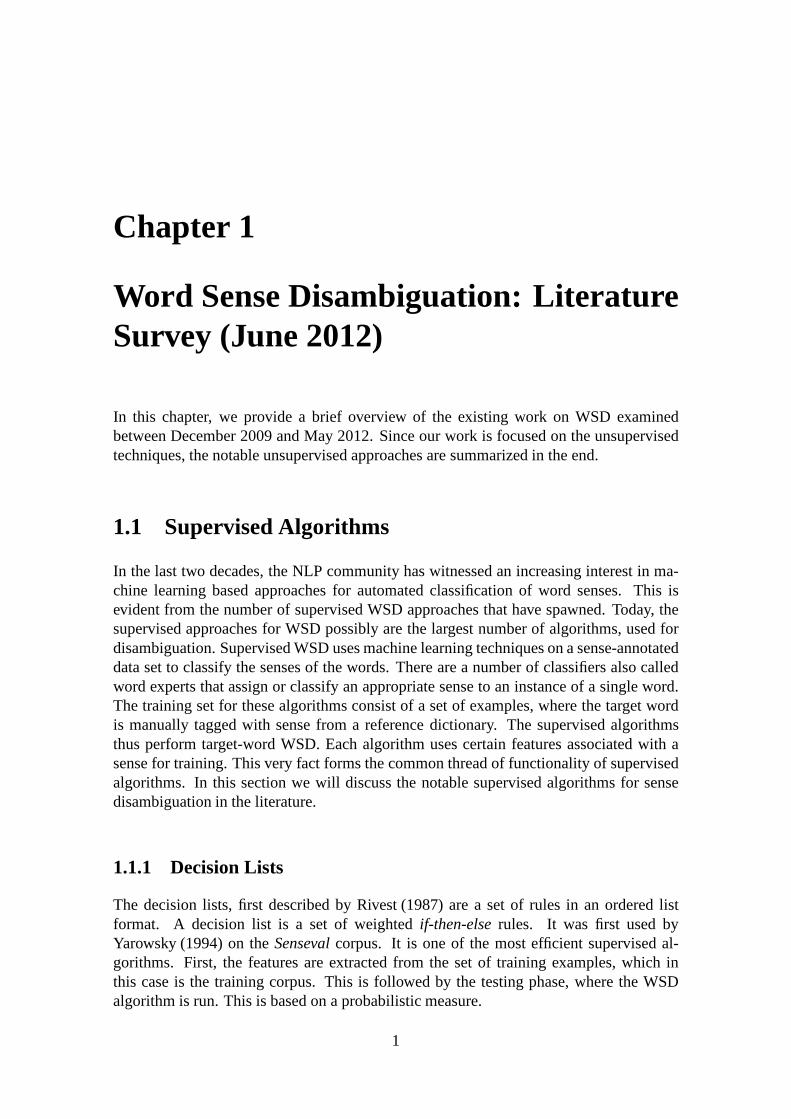
Chapter 1

Word Sense Disambiguation: LiteratureSurvey (June 2012)

In this chapter, we provide a brief overview of the existing work on WSD examinedbetween December 2009 and May 2012. Since our work is focusedon the unsupervisedtechniques, the notable unsupervised approaches are summarized in the end.

1.1 Supervised Algorithms

In the last two decades, the NLP community has witnessed an increasing interest in ma-chine learning based approaches for automated classification of word senses. This isevident from the number of supervised WSD approaches that have spawned. Today, thesupervised approaches for WSD possibly are the largest number of algorithms, used fordisambiguation. Supervised WSD uses machine learning techniques on a sense-annotateddata set to classify the senses of the words. There are a number of classifiers also calledword experts that assign or classify an appropriate sense toan instance of a single word.The training set for these algorithms consist of a set of examples, where the target wordis manually tagged with sense from a reference dictionary. The supervised algorithmsthus perform target-word WSD. Each algorithm uses certain features associated with asense for training. This very fact forms the common thread offunctionality of supervisedalgorithms. In this section we will discuss the notable supervised algorithms for sensedisambiguation in the literature.

1.1.1 Decision Lists

The decision lists, first described by Rivest (1987) are a setof rules in an ordered listformat. A decision list is a set of weightedif-then-elserules. It was first used byYarowsky (1994) on theSensevalcorpus. It is one of the most efficient supervised al-gorithms. First, the features are extracted from the set of training examples, which inthis case is the training corpus. This is followed by the testing phase, where the WSDalgorithm is run. This is based on a probabilistic measure.

1

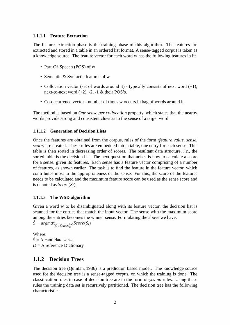
1.1.1.1 Feature Extraction

The feature extraction phase is the training phase of this algorithm. The features areextracted and stored in a table in an ordered list format. A sense-tagged corpus is taken asa knowledge source. The feature vector for each word w has thefollowing features in it:

• Part-Of-Speech (POS) of w

• Semantic & Syntactic features of w

• Collocation vector (set of words around it) - typically consists of next word (+1),next-to-next word (+2), -2, -1 & their POS’s.

• Co-occurrence vector - number of times w occurs in bag of words around it.

The method is based onOne sense per collocationproperty, which states that the nearbywords provide strong and consistent clues as to the sense of atarget word.

1.1.1.2 Generation of Decision Lists

Once the features are obtained from the corpus, rules of the form (feature value, sense,score)are created. These rules are embedded into a table, one entryfor each sense. Thistable is then sorted in decreasing order of scores. The resultant data structure,i.e., thesorted table is the decision list. The next question that arises is how to calculate a scorefor a sense, given its features. Each sense has a feature vector comprising of a numberof features, as shown earlier. The task is to find the feature in the feature vector, whichcontributes most to the appropriateness of the sense. For this, the score of the featuresneeds to be calculated and the maximum feature score can be used as the sense score andis denoted asScore(Si).

1.1.1.3 The WSD algorithm

Given a word w to be disambiguated along with its feature vector, the decision list isscanned for the entries that match the input vector. The sense with the maximum scoreamong the entries becomes the winner sense. Formulating theabove we have:S= argmax

Si∈Senses(w)DScore(Si)

Where:S= A candidate sense.D = A reference Dictionary.

1.1.2 Decision Trees

The decision tree (Quinlan, 1986) is a prediction based model. The knowledge sourceused for the decision tree is a sense-tagged corpus, on whichthe training is done. Theclassification rules in case of decision tree are in the form of yes-norules. Using theserules the training data set is recursively partitioned. Thedecision tree has the followingcharacteristics:

2

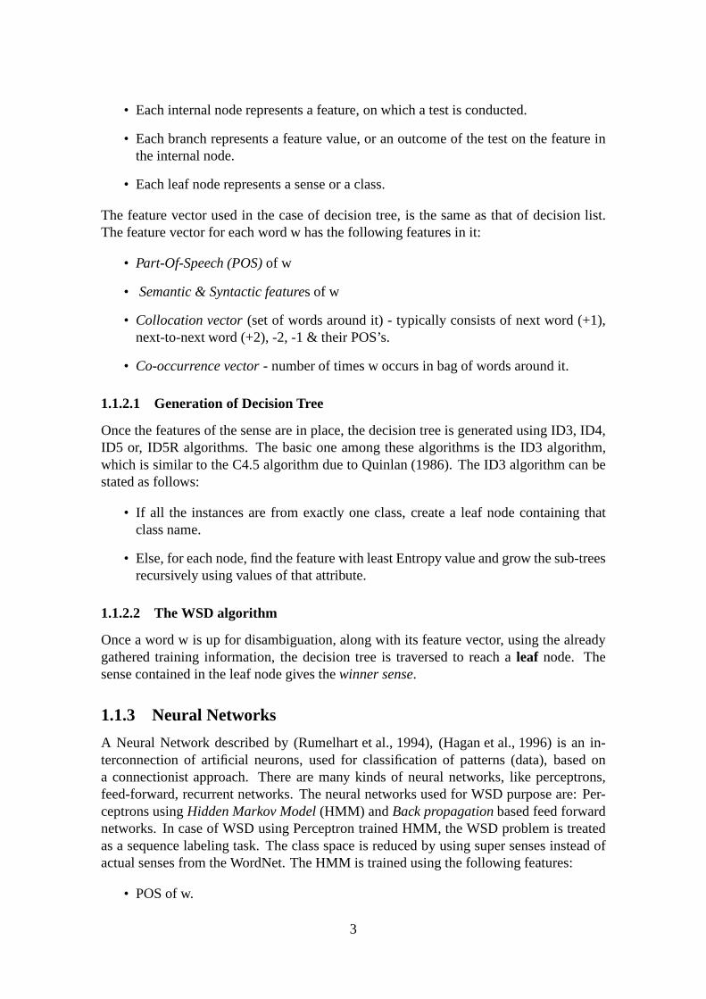
• Each internal node represents a feature, on which a test is conducted.

• Each branch represents a feature value, or an outcome of thetest on the feature inthe internal node.

• Each leaf node represents a sense or a class.

The feature vector used in the case of decision tree, is the same as that of decision list.The feature vector for each word w has the following featuresin it:

• Part-Of-Speech (POS)of w

• Semantic & Syntactic features of w

• Collocation vector(set of words around it) - typically consists of next word (+1),next-to-next word (+2), -2, -1 & their POS’s.

• Co-occurrence vector- number of times w occurs in bag of words around it.

1.1.2.1 Generation of Decision Tree

Once the features of the sense are in place, the decision treeis generated using ID3, ID4,ID5 or, ID5R algorithms. The basic one among these algorithms is the ID3 algorithm,which is similar to the C4.5 algorithm due to Quinlan (1986).The ID3 algorithm can bestated as follows:

• If all the instances are from exactly one class, create a leaf node containing thatclass name.

• Else, for each node, find the feature with least Entropy value and grow the sub-treesrecursively using values of that attribute.

1.1.2.2 The WSD algorithm

Once a word w is up for disambiguation, along with its featurevector, using the alreadygathered training information, the decision tree is traversed to reach aleaf node. Thesense contained in the leaf node gives thewinner sense.

1.1.3 Neural Networks

A Neural Network described by (Rumelhart et al., 1994), (Hagan et al., 1996) is an in-terconnection of artificial neurons, used for classification of patterns (data), based ona connectionist approach. There are many kinds of neural networks, like perceptrons,feed-forward, recurrent networks. The neural networks used for WSD purpose are: Per-ceptrons usingHidden Markov Model(HMM) and Back propagationbased feed forwardnetworks. In case of WSD using Perceptron trained HMM, the WSD problem is treatedas a sequence labeling task. The class space is reduced by using super senses instead ofactual senses from the WordNet. The HMM is trained using the following features:

• POS of w.

3

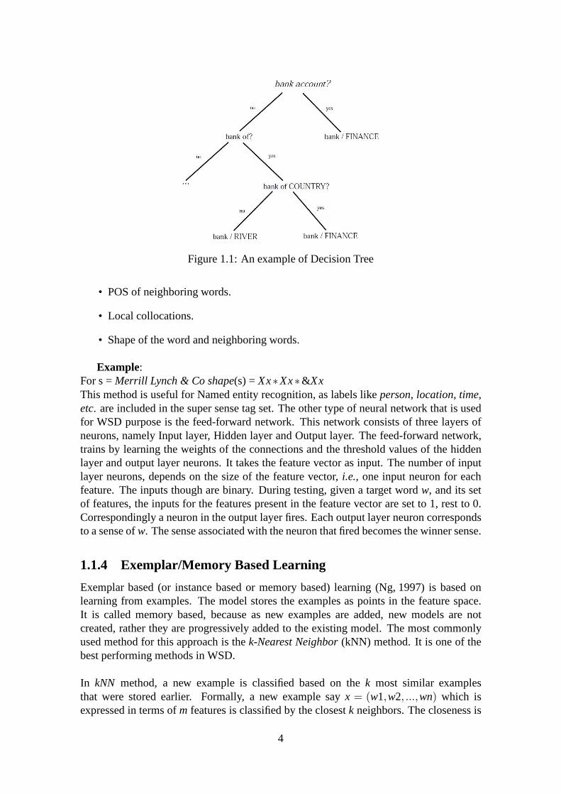
Figure 1.1: An example of Decision Tree

• POS of neighboring words.

• Local collocations.

• Shape of the word and neighboring words.

Example:For s =Merrill Lynch & Co shape(s) =Xx∗Xx∗&XxThis method is useful for Named entity recognition, as labels like person, location, time,etc. are included in the super sense tag set. The other type of neural network that is usedfor WSD purpose is the feed-forward network. This network consists of three layers ofneurons, namely Input layer, Hidden layer and Output layer.The feed-forward network,trains by learning the weights of the connections and the threshold values of the hiddenlayer and output layer neurons. It takes the feature vector as input. The number of inputlayer neurons, depends on the size of the feature vector,i.e., one input neuron for eachfeature. The inputs though are binary. During testing, given a target wordw, and its setof features, the inputs for the features present in the feature vector are set to 1, rest to 0.Correspondingly a neuron in the output layer fires. Each output layer neuron correspondsto a sense ofw. The sense associated with the neuron that fired becomes the winner sense.

1.1.4 Exemplar/Memory Based Learning

Exemplar based (or instance based or memory based) learning(Ng, 1997) is based onlearning from examples. The model stores the examples as points in the feature space.It is called memory based, because as new examples are added,new models are notcreated, rather they are progressively added to the existing model. The most commonlyused method for this approach is thek-Nearest Neighbor(kNN) method. It is one of thebest performing methods in WSD.

In kNN method, a new example is classified based on thek most similar examplesthat were stored earlier. Formally, a new example sayx = (w1,w2, ...,wn) which isexpressed in terms ofm features is classified by the closestk neighbors. The closeness is

4

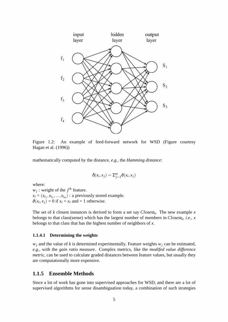
Figure 1.2: An example of feed-forward network for WSD (Figure courtesyHagan et al. (1996))

mathematically computed by the distance,e.g., theHamming distance:

δ(xi ,x j) = Σmj=1∂(xi ,x j)

where:w j : weight of thejth feature.xi = (xi1,xi2, ...,xim) : a previously stored example.∂(xi ,x j) = 0 if xi = xi and = 1 otherwise.

The set ofk closest instances is derived to form a set sayClosestk. The new examplexbelongs to that class(sense) which has the largest number ofmembers inClosestk, i.e., xbelongs to that class that has the highest number of neighbors ofx.

1.1.4.1 Determining the weights

w j and the value ofk is determined experimentally. Feature weightsw j can be estimated,e.g., with the gain ratio measure. Complex metrics, like themodifed value differencemetric, can be used to calculate graded distances between feature values, but usually theyare computationally more expensive.

1.1.5 Ensemble Methods

Since a lot of work has gone into supervised approaches for WSD, and there are a lot ofsupervised algorithms for sense disambiguation today, a combination of such strategies

5

Figure 1.3: An example of kNN on 2D plane (Figure courtesy Ng (1997))

could result in a highly efficient supervised approach and improve the overall accuracyof the WSD process. Features should actually be chosen so that significantly different,possibly independent, views of the training data (e.g., lexical, grammatical, semantic fea-tures,etc.) are formed. These combination strategies are called ensemble methods. Oneof the cheif ensemble methods is majority voting, describedbelow. The ensemble strategythat has highest accuracy is the AdaBoost method.

1.1.5.1 Majority Voting

In the majority voting scheme, each classifier votes for a particular sense of the givenword w. A classifier votes for a senseSi of the word w, if that sense is the output, or thewinner sense for that classifier. The sense with the majorityof votes becomes the winnersense for this method. Formally, given w, the senses of wSi and the ensemble componentsCj . The winner senseS is found out by the formula:

S= argmaxSi∈SensesD(w)| j : vote(Cj) = Si |

If there is a tie, then a random choice is made among the winnersenses or the ensembledoes not output anything.

1.1.5.2 AdaBoost

Adaboost is a theoretical framework of a machine learning model called ProbablyApproximately Correct(PAC). The method is sensitive to noisy data and outliers, andis consequently less susceptible to overfitting than other machine learning approaches.AdaBoost orAdaptive Boosting(Margineantu and Dietterich, 1997) constructs astrongclassifier by taking a linear combination of a number ofweakclassifiers. The method iscalled Adaptive because it tunes classifiers to correctly classify instances misclassifiedby previous classifiers.

6

For learning purposes, instances in the training data set are equally weighted initially.AdaBoost learns from this weighted training data set. Form ensemble components,ititeratesm times, one iteration for each classifier. In each iteration,the weights of themisclassified instances are increased, thus reducing theoverall classificationerror.

As a result of this method, after each iterationj = 1, ...,m a weightα j is obtained foreach classifierCj , which is a function of the classification error forCj , over the trainingset. Given the classifiersC1,C2, ...,Cm the attempt is to improveα j which is the weight orimportance of each classifier. The resultantstrongclassifier H can thus be formulated as:

H(x) = sign(Σmj=1α jCj(x))

This indicated thatH is the sign function of a linear combination of theweakclassifiers.An extension of AdaBoost which deals with multiclass, multilabel classification is Ad-aBoost.MH as demonstrated by Abney et al. (1999). An application of AdaBoost calledLazyBoostingwas also used by Escudero et al. (2001). LazyBoosting is essentially Ad-aBoost used for WSD purpose.

1.1.6 Support Vector Machines

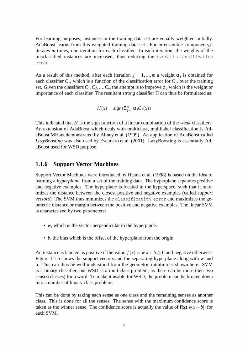
Support Vector Machines were introduced by Hearst et al. (1998) is based on the idea oflearning ahyperplane, from a set of the training data. The hyperplane separates positiveand negative examples. The hyperplane is located in the hyperspace, such that it max-imizes the distance between the closest positive and negative examples (calledsupportvectors). The SVM thus minimizes theclassification error and maximizes the ge-ometric distance or margin between the positive and negative examples. The linear SVMis characterized by two parameters:

• w, which is the vector perpendicular to the hyperplane.

• b, the bias which is the offset of the hyperplane from the origin.

An instance is labeled as positive if the valuef (x) = w.x+b≥ 0 and negative otherwise.Figure 1.1.6 shows the support vectors and the separating hyperplane along with w andb. This can thus be well understood from the geometric intuition as shown here. SVMis a binary classifier, but WSD is a multiclass problem, as there can be more then twosenses(classes) for a word. To make it usable for WSD, the problem can be broken downinto a number of binary class problems.

This can be done by taking each sense as one class and the remaining senses as anotherclass. This is done for all the senses. The sense with the maximum confidence score istaken as the winner sense. The confidence score is actually the value off(x)[w.x+b], foreach SVM.

7

Figure 1.4: The geometric intuition of SVM (Figure courtesyHearst et al. (1998))

1.1.7 SNoW Architecture

Snow stands forSparse Network Of Winnows, which is an online learning algorithm.The fundamental construct of the algorithm is theWinnow algorithm(Blum, 1995). Thealgorithm learns very fast in the presence of many binary input features, as it consistsof a linear threshold algorithm and updates multiplicativeweight for problems having 2classes (Carlson et al., 1999).

Each class in the SNoW architecture has a winnow node, which learns to separatethat class from the remaining classes. During training, if an example belongs to thecorresponding class, then it is considered positive for thewinnow node, else it is anegative example. The nodes are not connected to all features; rather they are connectedto “relevant” features for their class only. This accounts for the fast learning rate ofSNoW.

When classifying a new example, SNoW behaves somewhat like aneural net, whichtakes features as input and outputs the class with the highest activation value. Accordingto Blum (1995), SNoW performs well in higher dimensional domains. Both the targetfunction and the training instances are sparsely distributed in the feature space,e.g., textcategorization, context sensitive spelling correction, WSD,etc.

8

1.2 Semi-supervised Algorithms

Supervised algorithms train a model based on the annotated corpus provided to it. Thiscorpus needs to be manually annotated, and the size of the corpus needs to be largeenough in order to train a generalized model.

Semi-supervised, also known asminimally supervised algorithms make some assump-tions about the language and discourse in order to minimize these restrictions. Thecommon thread of operation of these algorithms are theseassumptions and theseedsused by them for disambiguation purposes.

This section presents two such approaches, based on two different ways to look at theproblem, namely Bootstrapping and Monosemous Relatives.

1.2.1 Bootstrapping

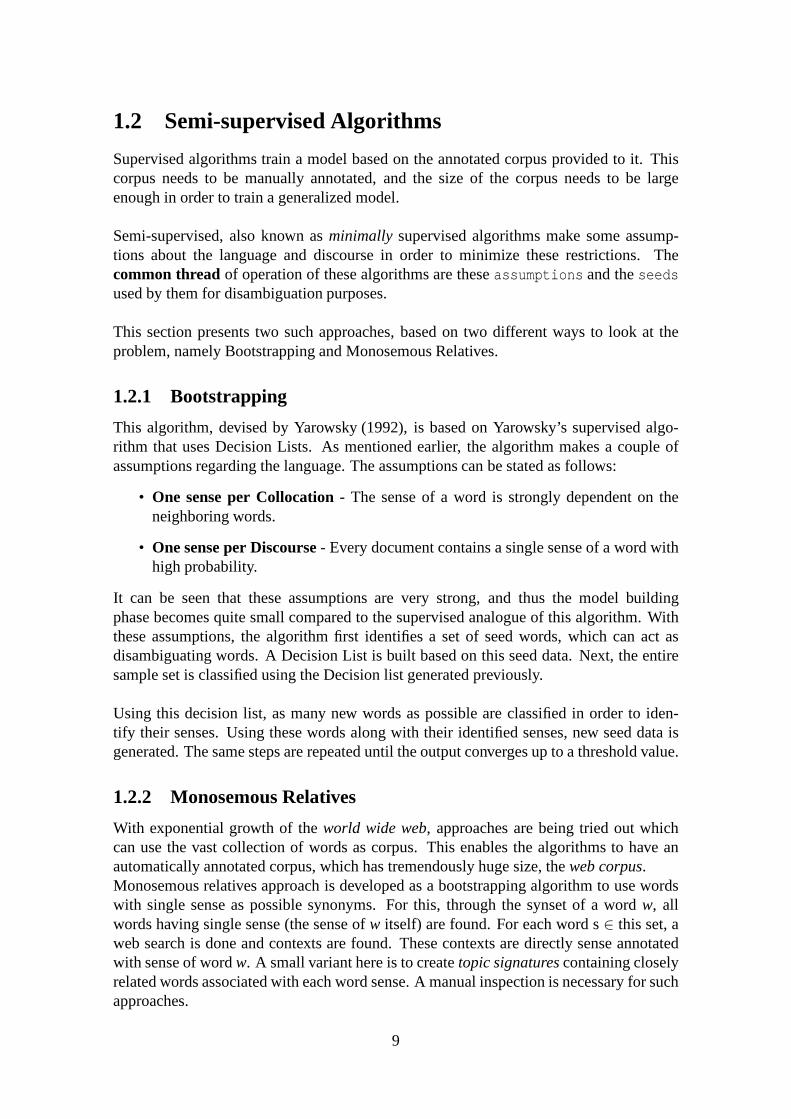
This algorithm, devised by Yarowsky (1992), is based on Yarowsky’s supervised algo-rithm that uses Decision Lists. As mentioned earlier, the algorithm makes a couple ofassumptions regarding the language. The assumptions can bestated as follows:

• One sense per Collocation - The sense of a word is strongly dependent on theneighboring words.

• One sense per Discourse - Every document contains a single sense of a word withhigh probability.

It can be seen that these assumptions are very strong, and thus the model buildingphase becomes quite small compared to the supervised analogue of this algorithm. Withthese assumptions, the algorithm first identifies a set of seed words, which can act asdisambiguating words. A Decision List is built based on thisseed data. Next, the entiresample set is classified using the Decision list generated previously.

Using this decision list, as many new words as possible are classified in order to iden-tify their senses. Using these words along with their identified senses, new seed data isgenerated. The same steps are repeated until the output converges up to a threshold value.

1.2.2 Monosemous Relatives

With exponential growth of theworld wide web, approaches are being tried out whichcan use the vast collection of words as corpus. This enables the algorithms to have anautomatically annotated corpus, which has tremendously huge size, theweb corpus.Monosemous relatives approach is developed as a bootstrapping algorithm to use wordswith single sense as possible synonyms. For this, through the synset of a wordw, allwords having single sense (the sense ofw itself) are found. For each word s∈ this set, aweb search is done and contexts are found. These contexts aredirectly sense annotatedwith sense of wordw. A small variant here is to createtopic signaturescontaining closelyrelated words associated with each word sense. A manual inspection is necessary for suchapproaches.

9

Figure 1.5: figure showing growth of Semi-supervised decision list on two senses of plantviz., life and manufacturing. (a) The initial seed data. (b) Growth of the seed set. (c) Seeddata converges. (Figure courtesy Yarowsky (1992))

1.3 Unsupervised algorithms

A Supervised approach in WSD needs training data on which it builds models orhypotheses. The training data has to be manually created, which is very expensive, bothtemporally and financially. This problem is typically knownasKnowledgeacquisitionbottleneck. Unsupervised algorithms overcome this problem by assuming that thesense of a word will depend on those of neighboring words. Thesingle commonthread which binds these algorithms is theclustering strategy used on the wordsinthe un-annotated corpus. The words are then classified into one of these clustersbased on some similarity measure. These algorithms are therefore termed asWordsense discrimination algorithmsrather than disambiguation algorithms. Althoughthey do not end up finding the actual sense of a word, the clustering and classificationenables one to label the senses, and therefore these approaches are treated as part of WSD.

Since the sense clusters derived by these algorithms may notmatch the actual sensesdefined in Lexical resources like dictionaries, the evaluation of these algorithms needsto be carried out manually, by asking language experts to corroborate the results. Basedon thetype of clustering performedby unsupervised algorithms, they can be classified asfollows:

1.3.1 Context clustering algorithms

Context is formally a discourse that surrounds a language unit (e.g.a word) and helps todetermine its interpretation. The algorithms in this domain represent the occurrences oftarget words as word vectors. From these vectors, context vectors are formed and meaningsimilarity is found that is a function of cosine between the context vectors:

10

sim(v,w) = v·w|v|·||w| =

∑mi=1 vi ·wi√

∑mi=1 v2

i

∑mi=1w2

i

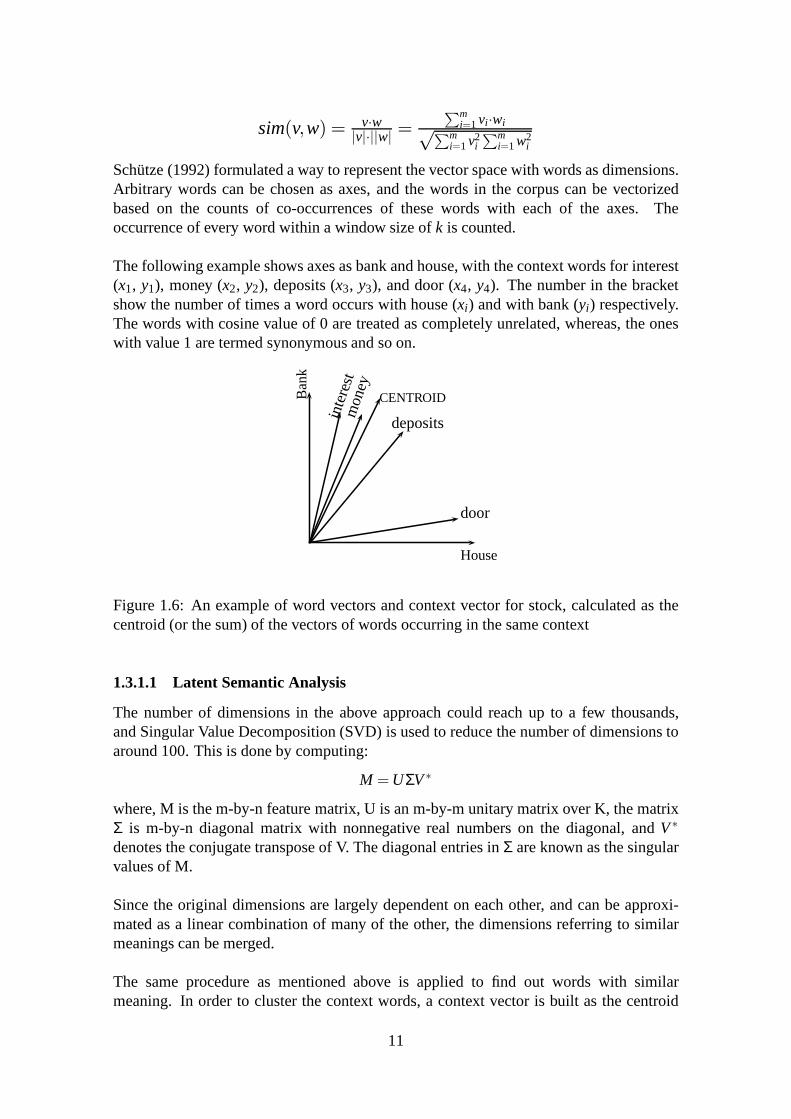
Schutze (1992) formulated a way to represent the vector space with words as dimensions.Arbitrary words can be chosen as axes, and the words in the corpus can be vectorizedbased on the counts of co-occurrences of these words with each of the axes. Theoccurrence of every word within a window size ofk is counted.

The following example shows axes as bank and house, with the context words for interest(x1, y1), money (x2, y2), deposits (x3, y3), and door (x4, y4). The number in the bracketshow the number of times a word occurs with house (xi) and with bank (yi) respectively.The words with cosine value of 0 are treated as completely unrelated, whereas, the oneswith value 1 are termed synonymous and so on.

CENTROID

inte

rest

mon

ey

deposits

door

House

Ban

k

Figure 1.6: An example of word vectors and context vector forstock, calculated as thecentroid (or the sum) of the vectors of words occurring in thesame context

1.3.1.1 Latent Semantic Analysis

The number of dimensions in the above approach could reach upto a few thousands,and Singular Value Decomposition (SVD) is used to reduce thenumber of dimensions toaround 100. This is done by computing:

M =UΣV∗

where, M is the m-by-n feature matrix, U is an m-by-m unitary matrix over K, the matrixΣ is m-by-n diagonal matrix with nonnegative real numbers on the diagonal, andV∗

denotes the conjugate transpose of V. The diagonal entries in Σ are known as the singularvalues of M.

Since the original dimensions are largely dependent on eachother, and can be approxi-mated as a linear combination of many of the other, the dimensions referring to similarmeanings can be merged.

The same procedure as mentioned above is applied to find out words with similarmeaning. In order to cluster the context words, a context vector is built as the centroid

11

of the word vectors which were found in the target context. The centroid finds theapproximation of semantic context. It can be seen that the centroid vector is a secondorder vector, as it does not represent the context directly.In the above figure, the centroidvector is shown for 3 wordsviz., interest, money, and deposits.

1.3.1.2 Context Group Discrimination

This algorithm, which is due to Schutze (1992), goes one step ahead to discriminatethe word senses after their context vectors are formed. Thisalgorithm was developedto cluster the senses of the words for which ambiguity is present in the corpus. Thealgorithm represents senses, words, and context in a multi-dimensional real-valued vectorspace.The clustering is done based on contextual similarities between the occurrences. Thecontextual similarities are still found with cosine function, but the clustering is done usingExpectation Maximization algorithm, an iterative, probabilistic model for maximumlikelihood estimation.

In the sense acquisition phase, the contexts of all the occurrences of the ambiguouswords are represented as context vectors as explained earlier, and a method calledaverage agglomerative clustering is used. The similarity is calculated as a function ofnumber of neighbors common to the words. The more similar words appear in the twocontexts, more similar the contexts become. After this, theoccurrences are grouped sothat occurrences with similar contexts are assigned to samecluster.

A very similar approach is followed in Structural Semantic Interconnections (hybrid al-gorithm).

1.3.2 Word Clustering Approaches

Context vectors previously explained, are second-order representations of wordsenses, as in they represent the senses indirectly. The ideahere is to cluster the sensesbased on word vectors, in order to draw out the semantic relationships between the words.

The notable algorithms in this section are:

1.3.2.1 Lin’s approach

Lin (1998) clusters two words if they share some syntactic relationship. More therelation, more close the words are situated in the cluster. Given context wordsw1, w2, · · ·,wn and a target word w, the similarity between w andwi is determined by the informationcontent of their syntactic features.The previous approach uses context vectors, which conflate senses of words, and thus,similarity of w with eachwi can not be determined with that approach. Therefore, eachword is represented in form of a vector. The information contents are then found outusing the syntactic features as mentioned previously.

12

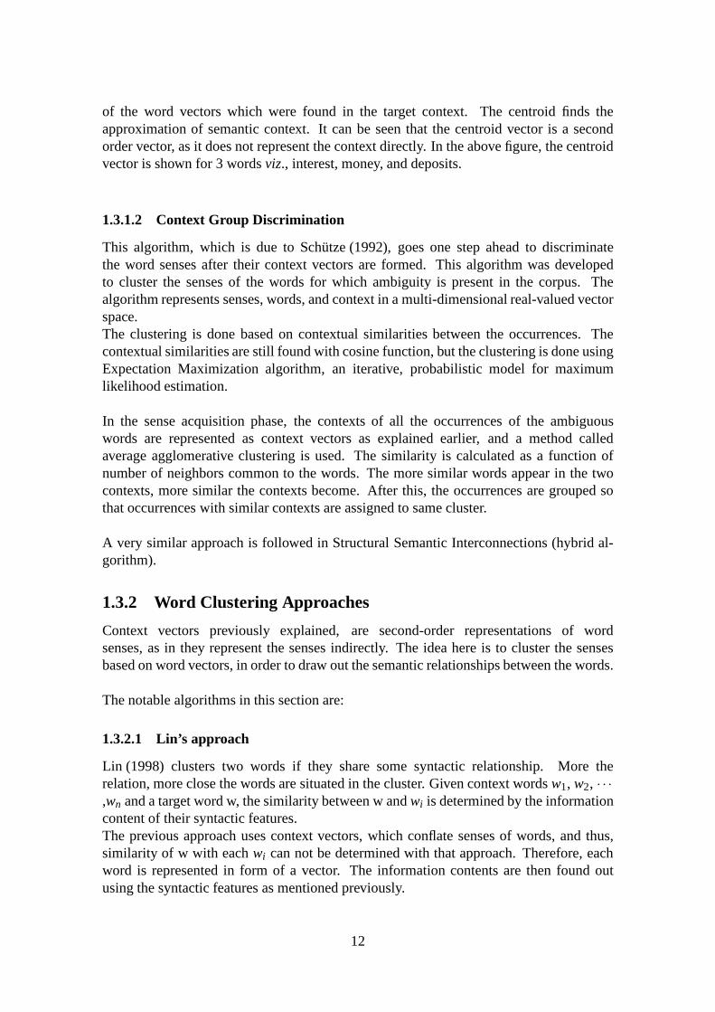
Example:The facility will employ 500 new employees.Here, the wordfacility is to be disambiguated (discriminated). From the corpus, the in-formation content of each subject of employ is determined interms of thelog likelihood.Since the sense ofinstallationfor facility has highest similarity with the major four sub-jects ofemploy(viz., org, plant, company, industry), it becomes the winner sense.

Senses of Facility Subjects of Employinstallation word freq log likelihoodproficiency org 64 51.7adeptness plant 14 33.0readiness company 27 29.9bathroom/toilet industry 9 15.4In this case Sense 1 of installationunit 9 10.2would be the winner sense. aerospace 2 6.3

Table 1.1: Table showing working of Lin’s approach. The winner sense is highlighted.

1.3.2.2 Clustering by Committee

This algorithm, again proposed by Pantel and Lin (2002), canbe viewed as an extensionover Lin’s original approach to WSD discussed previously. This algorithm follows thesame steps up to representing the words as a feature vector.After this, the algorithm recursively decides the clusters, referred to here ascommittees.Given a set of wordsW, the algorithm usesaverage link methodto cluster the words.In each step, the words are clustered based on their similarity to the centroids of thecommittees, and the words which are not similar are gathered. These words, referred tohere asresidue words, are used to discover more committees.

While disambiguating a wordw, the word is represented using its feature vector and themost similar committee is found for this word.

The algorithm can be summarized as below:

1. Find K nearest neighbors (kNN) for each element,for some small value of k.

2. Form clusters using the kNN obtained from step 1.

3. For every new instance e input to the system,assign it to its nearest cluster, as per averagelink method.

Typically, the value ofk is selected to be between 10 and 20. The elements of each clusterare called acommittee.

13

1.3.3 Co-occurrence Graphs

Whereas the previous techniques use vectors to represent the words, the algorithms inthis domain make use of graphs. Every word in the text becomesa vertex and syntacticrelations become edges. The context units (e.g. paragraph) in which the target wordsoccur, are used to create the graphs.

The algorithm worth mentioning here is Hyperlex, as proposed by Veronis (2004).

1.3.3.1 Hyperlex

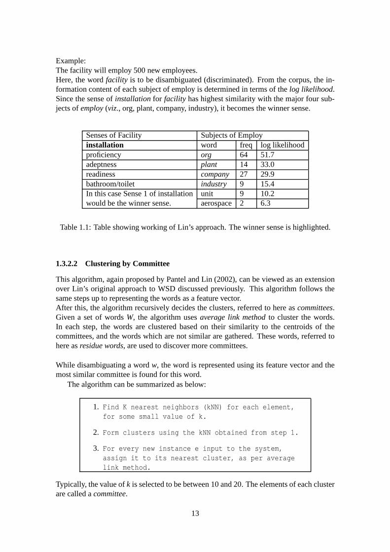
As per this algorithm, the words in context (e.g. in the same paragraph) with the targetword become vertices, and they are joined with an edge, if they co-occur in sameparagraph. The edge weights are inversely proportional to the frequency of co-occurrenceof these words.

wi j = 1 - max{

P(wi |w j),P(w j |wi)}

where,P(wi | w j) =Frequency o f co−occurrence o f words wi and wj

Frequency o f occurrence o f wjIt can be seen that as an implication, words which co-occur with high frequency, get anedge weight of close to 0 and the other extreme gets 1.

Figure 1.7: Hyperlex showing (a) Part of a co-occurrence graph. (b) The minimum span-ning tree for the target wordbar. (Figure courtesy Navigli (February 2009))

After this is done, iteratively the node with highest relative degree (number of connec-tions) in the graph is selected as a hub. Once this is done, theneighbors of this nodecease to be candidates of being hubs. The relative degree forremaining nodes is againcomputed and this is iterated until the highest relative degree reaches some predefinedthreshold. The hubs are then linked to the ambiguous word by finding MinimumSpanning Tree (MST) for the resultant graph.

Each node in the MST is assigned a score vector s with as many dimensions as there arecomponents:

14

s=

{

11+d(hi,v)

i f v ∈ component i

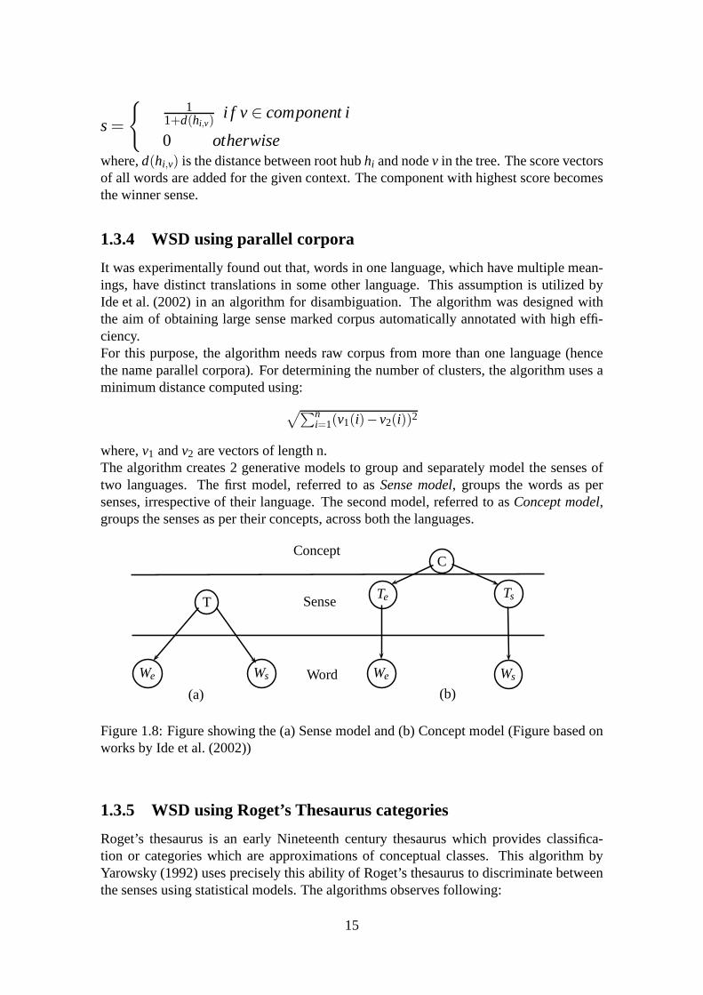
0 otherwisewhere,d(hi,v) is the distance between root hubhi and nodev in the tree. The score vectorsof all words are added for the given context. The component with highest score becomesthe winner sense.

1.3.4 WSD using parallel corpora

It was experimentally found out that, words in one language,which have multiple mean-ings, have distinct translations in some other language. This assumption is utilized byIde et al. (2002) in an algorithm for disambiguation. The algorithm was designed withthe aim of obtaining large sense marked corpus automatically annotated with high effi-ciency.For this purpose, the algorithm needs raw corpus from more than one language (hencethe name parallel corpora). For determining the number of clusters, the algorithm uses aminimum distance computed using:

√

∑ni=1(v1(i)−v2(i))2

where,v1 andv2 are vectors of length n.The algorithm creates 2 generative models to group and separately model the senses oftwo languages. The first model, referred to asSense model, groups the words as persenses, irrespective of their language. The second model, referred to asConcept model,groups the senses as per their concepts, across both the languages.

C

Te Ts

We Ws

T

We Ws

Concept

Sense

Word

(a) (b)

Figure 1.8: Figure showing the (a) Sense model and (b) Concept model (Figure based onworks by Ide et al. (2002))

1.3.5 WSD using Roget’s Thesaurus categories

Roget’s thesaurus is an early Nineteenth century thesauruswhich provides classifica-tion or categories which are approximations of conceptual classes. This algorithm byYarowsky (1992) uses precisely this ability of Roget’s thesaurus to discriminate betweenthe senses using statistical models. The algorithms observes following:

15

• Different conceptual classes of words tend to appear in recognizably different con-texts.

• Different word senses belong to different conceptual classes.

• A context based discriminator for the conceptual classes can serve as a contextbased discriminator for the members of those classes.

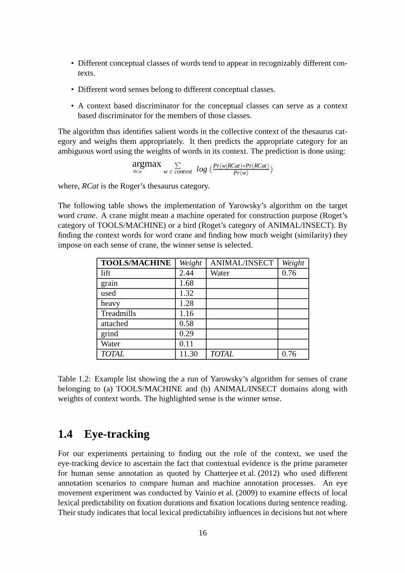
The algorithm thus identifies salient words in the collective context of the thesaurus cat-egory and weighs them appropriately. It then predicts the appropriate category for anambiguous word using the weights of words in its context. Theprediction is done using:

argmaxRCat

∑

w∈ context log (Pr(w|RCat)∗Pr(RCat)Pr(w) )

where,RCatis the Roger’s thesaurus category.

The following table shows the implementation of Yarowsky’salgorithm on the targetword crane. A crane might mean a machine operated for construction purpose (Roget’scategory of TOOLS/MACHINE) or a bird (Roget’s category of ANIMAL/INSECT). Byfinding the context words for word crane and finding how much weight (similarity) theyimpose on each sense of crane, the winner sense is selected.

TOOLS/MACHINE Weight ANIMAL/INSECT Weightlift 2.44 Water 0.76grain 1.68used 1.32heavy 1.28Treadmills 1.16attached 0.58grind 0.29Water 0.11TOTAL 11.30 TOTAL 0.76

Table 1.2: Example list showing the a run of Yarowsky’s algorithm for senses of cranebelonging to (a) TOOLS/MACHINE and (b) ANIMAL/INSECT domains along withweights of context words. The highlighted sense is the winner sense.

1.4 Eye-tracking

For our experiments pertaining to finding out the role of the context, we used theeye-tracking device to ascertain the fact that contextual evidence is the prime parameterfor human sense annotation as quoted by Chatterjee et al. (2012) who used differentannotation scenarios to compare human and machine annotation processes. An eyemovement experiment was conducted by Vainio et al. (2009) toexamine effects of locallexical predictability on fixation durations and fixation locations during sentence reading.Their study indicates that local lexical predictability influences in decisions but not where

16

the initial fixation lands in a word.

In another work based on word grouping hypothesis and eye movements during readingby Drieghe et al. (2008), the distribution of landing positions and durations of first fix-ations in a region containing a noun preceded by either an article or a high-frequencythree-letter word were compared. In our current work we use eye-tracking as a tool tomake findings regarding the cognitive processes connected to the human sense disam-biguation procedure, and to gain a better understanding of “contextual evidence” whichis of paramount importance for human annotation. Unfortunately, our work seems to bea first of its kind, as to the best of our knowledge we do not knowof any such work donebefore in the literature.

1.5 Summary of notable Unsupervised WSD approaches

1.5.1 Monolingual WSD

Depending on the type of evidence or knowledge sources used,existing algorithms formonlingual WSD can be classified into two broad categories,viz., knowledge basedapproaches and machine learning based approaches. Machinelearning based approachescan be further divided into supervised (require sense tagged corpus), unsupervised(require untagged corpus) and semi-supervised approaches(bootstrap using a smallamount of tagged corpus and a large amount of untagged corpus).

Knowledge based approaches to WSD such as Lesk (1986), Walker and Amsler (1986),conceptual density by Agirre and Rigau (1996) and random walk algorithm byRada (2005) essentially do Machine Readable Dictionary lookup. However, these arefundamentallyoverlap basedalgorithms which suffer from overlap sparsity, dictionarydefinitions being generally small in length.

Supervised learning algorithms for WSD are mostly word specific classifiers, e.g.,Lee Yoong K. and Chia (2004), Ng and Lee (1996) and Yarowsky (1994). The require-ment of a large training corpus renders these algorithms unsuitable for resource scarcelanguages.

Semi-supervised and unsupervised algorithms do not need large amount of annotatedcorpora, but are again word specific classifiers,e.g., semi-supervised decision list al-gorithm by Yarowsky (1995) and Hyperlex by Veronis (2004). Hybrid approaches likeWSD using Structural Semantic Interconnections as shown inNavigli and Velardi (2005)use combinations of more than one knowledge sources (WordNet as well as a smallamount of tagged corpora). This allows them to capture important information encodedin Fellbaum (1998) as well as draw syntactic generalizations from minimally tagged cor-pora. These methods which combine evidence from several resources seem to be mostsuitable in building general purpose broad coverage disambiguation engines and are themotivation for our work.

17

1.5.2 Bilingual WSD

The limited performance of monolingual approaches to deliver high accuracies for all-words WSD at low costs created interest in bilingual approaches which aim at reducingthe annotation effort. Here again, the approaches can be classified into two categories,viz., (i) approaches using parallel corpora and (ii) approachesnot using parallel corpora.

The approaches which use parallel corpora rely on the paradigm of Disambigua-tion by Translation, described in the works of Gale et al. (1992), Dagan and Itai (1994),Resnik and Yarowsky (1999), Ide et al. (2001), Diab and Resnik (2002), Ng et al. (2003),Tufis et al. (2004), Apidianaki (2008). Such algorithms relyon the frequently madeobservation that a word in a given source language tends to have different translationsin a target language depending on its sense. Given a sentence-and-word-aligned parallelcorpus, these different translations in the target language can serve as automaticallyacquired sense labels for the source word.

In this work, we are more interested in the second kind of approaches which do not useparallel corpora but rely purely on the in-domain corpora from two (or more) languages.For example, Li and Li (2004) proposed a bilingual bootstrapping approach for the morespecific task of Word Translation Disambiguation (WTD) as opposed to the more generaltask of WSD. This approach does not need parallel corpora (just like our approach) andrelies only on in-domain corpora from two languages. However, their work was evaluatedonly on a handful of target words (9 nouns) for WTD as opposed to our work whichfocuses on the broader task of all-words WSD.

Another approach worth mentioning here is the one proposed byKaji and Morimoto (2002) which aligns statistically significant pairs of related wordsin languageL1 with their cross-lingual counterparts in languageL2 using a bilingualdictionary. This approach is based on two assumptions (i) words which are mostsignificantly related to a target word provide clues about the sense of the target wordand (ii) translations of these related words further reinforce the sense distinctions. Thetranslations of related words thus act as cross-lingual clues for disambiguation. Thisalgorithm when tested on 60 polysemous words (using Englishas L1 and Japanese asL2) delivered high accuracies (coverage=88.5% and precision=77.7%). However, whentested in an all-words scenario, the approach performed waybelow the random baseline.

18

Bibliography

[Abney et al.1999] S. Abney, R.E. Schapire, and Y. Singer. 1999. Boosting appliedto tagging and pp attachment. InProceedingsof the Joint SIGDAT ConferenceonEmpiricalMethodsin NaturalLanguageProcessingandVery LargeCorpora, volume130, pages 132–134.

[Agirre and Rigau1996] Eneko Agirre and German Rigau. 1996.Word sense dis-ambiguation using conceptual density. InIn Proceedingsof the 16th InternationalConferenceonComputationalLinguistics(COLING).

[Apidianaki2008] Marianna Apidianaki. 2008. Translation-oriented word sense induc-tion based on parallel corpora. InLREC.

[Blum1995] A. Blum. 1995. Empirical support for winnow and weighted-majority algo-rithms: results on a calendar scheduling domain. InMachineLearning. Citeseer.

[Carlson et al.1999] A. Carlson, C. Cumby, J. Rosen, and D. Roth. 1999. The snowlearning architecture. Technical report, Technical report UIUCDCS.

[Chatterjee et al.2012] Arindam Chatterjee, Salil Joshi, Pushpak Bhattacharyya, DipteshKanojia, and Akhlesh Meena. 2012. A study of the sense annotation process: Man v/smachine.InternationalConferenceon GlobalWordnets, January.

[Dagan and Itai1994] Ido Dagan and Alon Itai. 1994. Word sense disambiguation usinga second language monolingual corpus.Comput.Linguist., 20:563–596, December.

[Diab and Resnik2002] Mona Diab and Philip Resnik. 2002. An unsupervised methodfor word sense tagging using parallel corpora. InProceedingsof the 40th AnnualMeetingonAssociationfor ComputationalLinguistics, ACL ’02, pages 255–262, Mor-ristown, NJ, USA. Association for Computational Linguistics.

[Drieghe et al.2008] D Drieghe, A Pollatsek, A Staub, and K Rayner. 2008. The wordgrouping hypothesis and eye movements during reading.

[Escudero et al.2001] G. Escudero, L. Marquez, and G. Rigau. 2001. Using lazyboost-ing for word sense disambiguation. InProceedingsof 2nd InternationalWorkshop“EvaluatingWord SenseDisambiguationSystems”,SENSEVAL-2.Toulouse.

[Fellbaum1998] C Fellbaum. 1998. Wordnet:an electronic lexical database. The MITPress.

19

[Gale et al.1992] William Gale, Kenneth Church, and David Yarowsky. 1992. A methodfor disambiguating word senses in a large corpus.Computersand the Humanities,26:415–439. 10.1007/BF00136984.

[Hagan et al.1996] M.T. Hagan, H.B. Demuth, M.H. Beale, and Boulder University ofColorado. 1996.Neuralnetworkdesign. PWS Pub.

[Hearst et al.1998] M.A. Hearst, ST Dumais, E. Osman, J. Platt, and B. Scholkopf. 1998.Support vector machines.IntelligentSystemsandtheirApplications,IEEE, 13(4):18–28.

[Ide et al.2001] Nancy Ide, Tomaz Erjavec, and Dan TufiS. 2001. Automatic sense tag-ging using parallel corpora. InIn Proceedingsof the6 thNaturalLanguageProcessingPacificRim Symposium, pages 212–219.

[Ide et al.2002] Nancy Ide, Tomaz Erjavec, and Dan Tufis. 2002. Sense discrimina-tion with parallel corpora. InProceedingsof the ACL-02 workshopon Word sensedisambiguation, pages 61–66, Morristown, NJ, USA. Association for ComputationalLinguistics.

[Kaji and Morimoto2002] Hiroyuki Kaji and Yasutsugu Morimoto. 2002. Unsupervisedword sense disambiguation using bilingual comparable corpora. InProceedingsof the19thinternationalconferenceon Computationallinguistics- Volume 1, COLING ’02,pages 1–7, Stroudsburg, PA, USA. Association for Computational Linguistics.

[Lee Yoong K. and Chia2004] Hwee T. Ng Lee Yoong K. and Tee K. Chia. 2004. Super-vised word sense disambiguation with support vector machines and multiple knowl-edge sources. InProceedingsof Senseval-3:Third InternationalWorkshopon theEvaluationof Systemsfor theSemanticAnalysisof Text, pages 137–140.

[Lesk1986] Michael Lesk. 1986. Automatic sense disambiguation using machine read-able dictionaries: how to tell a pine cone from an ice cream cone. InIn Proceedingsofthe5th annualinternationalconferenceonSystemsdocumentation.

[Li and Li2004] Hang Li and Cong Li. 2004. Word translation disambiguation usingbilingual bootstrapping.Comput.Linguist., 30:1–22, March.

[Lin1998] Dekang Lin. 1998. Automatic retrieval and clustering of similar words. InProceedingsof the17th internationalconferenceon Computationallinguistics, pages768–774, Morristown, NJ, USA. Association for Computational Linguistics.

[Margineantu and Dietterich1997] D.D. Margineantu and T.G. Dietterich. 1997. Prun-ing adaptive boosting. InMACHINE LEARNING-INTERNATIONAL WORKSHOPTHEN CONFERENCE-, pages 211–218. MORGAN KAUFMANN PUBLISHERS,INC.

[Navigli and Velardi2005] Roberto Navigli and Paolo Velardi. 2005. Structural seman-tic interconnections: A knowledge-based approach to word sense disambiguation. InIEEETransactionsOn PatternAnalysisandMachineIntelligence.

20

[NavigliFebruary 2009] Roberto Navigli. February 2009. Word sense disambiguation:A survey. InACM ComputingSurveys,Vol. 41,No. 2,Article 10.

[Ng and Lee1996] Hwee Tou Ng and Hian Beng Lee. 1996. Integrating multiple knowl-edge sources to disambiguate word sense: an exemplar-basedapproach. InProceedingsof the 34thannualmeetingon Associationfor ComputationalLinguistics, pages 40–47, Morristown, NJ, USA. Association for Computational Linguistics.

[Ng et al.2003] Hwee Tou Ng, Bin Wang, and Yee Seng Chan. 2003.Exploiting paralleltexts for word sense disambiguation: an empirical study. InProceedingsof the 41stAnnualMeetingon Associationfor ComputationalLinguistics- Volume 1, ACL ’03,pages 455–462, Morristown, NJ, USA. Association for Computational Linguistics.

[Ng1997] H.T. Ng. 1997. Exemplar-based word sense disambiguation: Some recentimprovements. InProceedingsof the SecondConferenceon Empirical methodsinnaturalLanguageProcessing, pages 208–213.

[Pantel and Lin2002] Patrick Pantel and Dekang Lin. 2002. Discovering word sensesfrom text. In KDD ’02: Proceedingsof the eighth ACM SIGKDD internationalconferenceonKnowledgediscoveryanddatamining, pages 613–619, New York, NY,USA. ACM.

[Quinlan1986] J. R. Quinlan. 1986. Induction of decision trees. Mach.Learn, pages81–106.

[Rada2005] Mihalcea Rada. 2005. Large vocabulary unsupervised word sense disam-biguation with graph-based algorithms for sequence data labeling. InIn ProceedingsoftheJointHumanLanguageTechnologyandEmpiricalMethodsin NaturalLanguageProcessingConference(HLT/EMNLP), pages 411–418.

[Resnik and Yarowsky1999] Philip Resnik and David Yarowsky. 1999. Distinguishingsystems and distinguishing senses: new evaluation methodsfor word sense disam-biguation.Nat.Lang.Eng., 5:113–133, June.

[Rivest1987] Ronald L. Rivest. 1987. Learning decision lists. In MachineLearning,pages 229–246.

[Rumelhart et al.1994] D.E. Rumelhart, B. Widrow, and M.A. Lehr. 1994. The basicideas in neural networks.Communicationsof theACM, 37(3):87–92.

[Schutze1992] H. Schutze. 1992. Dimensions of meaning. In Supercomputing’92:Proceedingsof the1992ACM/IEEE conferenceon Supercomputing, pages 787–796,Los Alamitos, CA, USA. IEEE Computer Society Press.

[Tufis et al.2004] Dan Tufis, Radu Ion, and Nancy Ide. 2004. Fine-grained word sensedisambiguation based on parallel corpora, word alignment,word clustering and alignedwordnets. InProceedingsof the 20th internationalconferenceon ComputationalLinguistics, COLING ’04, Stroudsburg, PA, USA. Association for Computational Lin-guistics.

21

[Vainio et al.2009] S. Vainio, J. Hyona, and A. Pajunen. 2009. Lexical predictabilityexerts robust effects on fixation duration, but not on initial landing position duringreading. volume 56, pages 66–74.

[Veronis2004] Jean Veronis. 2004. Hyperlex: Lexical cartography for information re-trieval. InComputerSpeechandLanguage, volume 18, pages 18(3):223–252.

[Walker and Amsler1986] D. Walker and R. Amsler. 1986. The use of machine readabledictionaries in sublanguage analysis. InIn AnalyzingLanguagein RestrictedDomains,Grish-manandKittredge(eds),LEA Press, pages 69–83.

[Yarowsky1992] David Yarowsky. 1992. Word-sense disambiguation using statisticalmodels of roget’s categories trained on large corpora. InProceedingsof the 14thconferenceon Computationallinguistics, pages 454–460, Morristown, NJ, USA. As-sociation for Computational Linguistics.

[Yarowsky1994] David Yarowsky. 1994. Decision lists for lexical ambiguity resolution:Application to accent restoration in spanish and french. InIn Proceedingsof the32ndAnnualMeetingof theassociationfor ComputationalLinguistics(ACL), pages 88–95.

[Yarowsky1995] David Yarowsky. 1995. Unsupervised word sense disambiguation ri-valing supervised methods. InProceedingsof the33rdannualmeetingon Associationfor ComputationalLinguistics, pages 189–196, Morristown, NJ, USA. Association forComputational Linguistics.

22