1

Nerve Excitation L. David Roper

http://arts.bev.net/roperldavid This is web page http://www.roperld.com/science/NerveExcitation.pdf

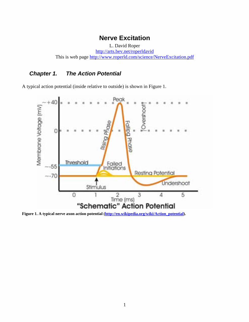
Chapter 1. The Action Potential A typical action potential (inside relative to outside) is shown in Figure 1.

Figure 1. A typical nerve axon action potential (http://en.wikipedia.org/wiki/Action_potential).

2

The explanation for the action potential, which once generated travels down the nerve axon with a speed of 10 to 100 meters/second, is as follows: • A resting electric potential of about -70 milliVolts (mV) inside relative to outside exists due to

approximate concentration differences across the squid giant-axon lipid membrane as follows: o 400 millimoles/liter (mM/l) inside and 20 mM/l outside for K+ ions. o 50 mM/l inside and 440 mM/l outside for Na+ ions. o About 100 mM/l inside and 560 mM/l outside for Cl- ions. o There are other ions present, such as Ca++, with concentration gradients across the

membrane. o The main cause of the -65 mV resting potential is that the membrane is mainly permeable to

K+ ions at rest, so that some K+ ions migrate to the outside setting up the potential. • An applied positive transient electric potential inside relative to outside above a threshold value

(about 40 mV) triggers a brief opening of a channel that allows Na+ ions to pass into the axon, causing the membrane potential to transiently move positively.

• That is followed by a brief opening of a channel that allows a greater flow of K+ ions outside the axon, which typically causes an overshoot below the resting potential

• Eventually the membrane potential restores to the resting potential, unless the stimulating potential is maintained, in which case, after a refractory period, it is repeated.

The time dependence of the “action potential” across the excitable membrane of the axon of a nerve cell can be represented by a combination of several hyperbolic tangents. (See http://en.wikipedia.org/wiki/Action_potential, http://en.wikipedia.org/wiki/Membrane_potential, http://en.wikipedia.org/wiki/Nernst_equation, http://en.wikipedia.org/wiki/Axon, and http://en.wikipedia.org/wiki/Hodgkin-huxley_model .) The opening of the two ion channels can be represented mathematically by two double hyperbolic tangents:

( ) Na1 Na 2 K1 K2

Na KNa1 Na 2 K1 K2

+

1 1tanh tanh tanh tanh ,2 2

where K resting potential.

r

r

t t t t t t t tV t V C Cw w w w

V

⎡ ⎤ ⎡ ⎤⎛ ⎞ ⎛ ⎞ ⎛ ⎞ ⎛ ⎞− − − −= + − + −⎢ ⎥ ⎢ ⎥⎜ ⎟ ⎜ ⎟ ⎜ ⎟ ⎜ ⎟

⎝ ⎠ ⎝ ⎠⎝ ⎠ ⎝ ⎠ ⎣ ⎦⎣ ⎦=

(1.1)

The hyperbolic-tangent function is a natural function to use for situations such as nerve excitation where a system changes from one state to another. In this case both the sodium and potassium ions have molecular channels across the axon membrane which change from one conductance state to another and then back to the original conductance state. The time interval between the turning on and off of the middle state may be so small that the full conductance is never realized because there are time constants (inverse of the rates) for turning on and off a conductance state. That is, there is a time constant for all channels changing from one state to another. It is more physical to use the hyperbolic-tangent function than the exponential function for state changes, because an exponential rise or fall cannot continue forever. Eventually there must be an asymptote, which the hyperbolic tangent provides.

3

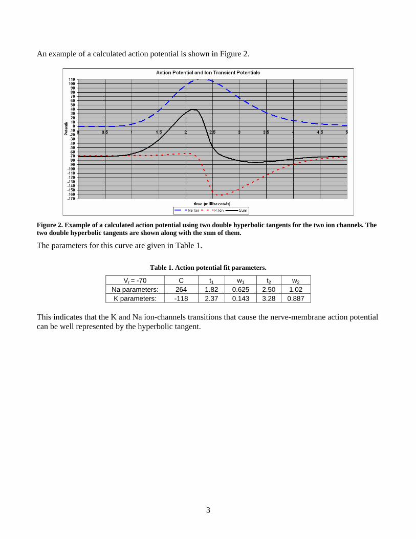
An example of a calculated action potential is shown in Figure 2.

Figure 2. Example of a calculated action potential using two double hyperbolic tangents for the two ion channels. The two double hyperbolic tangents are shown along with the sum of them.

The parameters for this curve are given in Table 1.

Table 1. Action potential fit parameters.

Vr = -70 C t1 w1 t2 w2 Na parameters: 264 1.82 0.625 2.50 1.02 K parameters: -118 2.37 0.143 3.28 0.887

This indicates that the K and Na ion-channels transitions that cause the nerve-membrane action potential can be well represented by the hyperbolic tangent.

4

One can create many different shapes for action potentials by varying the ten parameters in the equation. Figure 3 shows an example of a different shape.

Figure 3. Example of a calculated action potential using two double hyperbolic tangents for the two ion channels. The two double hyperbolic tangents are shown along with the sum of them.

The parameters for this curve are given in Table 2.

Table 2. Action potential parameters.

Vr = -70 C t1 w1 t2 w2 Na parameters: 300 2 0.5 4 0.75 K parameters: -100 3 0.1 4 0.4

These curves do not contain the transient stimulus electric potential of about +40 mV. It can be subtracted out from the measurement. It could be added to the equation as another double hyperbolic tangent. If more ions are involved with channels opening, such as Ca++, they can be added as another double hyperbolic tangent. It would be interesting to try to obtain an approximation to the Hodgkin-Huxley equations (http://biolpc22.york.ac.uk/hh/hh_excel.html) for the action potential by mathematically manipulating the equation given here.

5

Chapter 2. Voltage-Clamp Data Experiments can be arranged for the squid giant axon that fix the electric potential (voltage) across the membrane at different values. (http://en.wikipedia.org/wiki/Voltage_clamp) I use the data shown in Figure 7 on p. 36 of Hille (Hille, 1984). The data are for a membrane resting potential of 60 mV , opposite of the convention used in the action-potential calculation above. As Hille describes, it is well known that the current density (current/area = mA/cm2) consists of a potassium current density (JK) and a sodium current density (JNa). Here the former is parameterized by a hyperbolic tangent and the latter by two hyperbolic tangents, similar to what was used in the action-potential calculation above:

( ) ( ) ( ) ( ) ( ) ( )K Na 1 2, tanh tanh tanh .K Na NaJ t V J V r V t J V r V t r V t⎡ ⎤= + −⎡ ⎤ ⎡ ⎤ ⎡ ⎤⎣ ⎦ ⎣ ⎦ ⎣ ⎦⎣ ⎦ (1.2) (Note that the initial time is t=0 and tanh(at)=0 when t=0.) The voltage dependence of the parameters is indicated by, for example, ( )Kr V . That is, the K current density changes from one value to another and the Na current density transiently changes negatively, but then goes back to its original value. Another way to say it is that more K channels in the membrane open up and Na channels transiently open. Seven different voltages were fitted with this equation with five types of parameters, yielding the 35 parameters given in Table 3.

Table 3. Fit parameters at the different voltages for Eq. (1.2).

Potential -30 mV -10 mV 10 mV 30 mV 50 mV 70 mV 90 mV ( )KJ V -0.0688 1.294 1.259 1.653 2.172 2.716 3.215 ( )Kr V -0.3034 0.04868 0.1900 3.256 1.463 3.469 4.439 ( )NaJ V -86.78 -2.807 -1.937 3.296 4.136 5.164 5.447 ( )Na1r V 0.5133 2.450 6.590 0.3862 0.5693 0.6575 0.7446 ( )2Nar V 0.50535 0.4866 0.4631 3.255 1.462 1.885 2.058

Chi Sq. 0.00838 0.00700 0.00630 0.0233 0.0161 0.01106 0.00740 The total Chi Square is 0.0796 for fitting 224 data with 35 parameters. The fit was done by using the Solver routine in the Excel spreadsheet to minimize least squares between the data array and the array calculated using the fitting parameters.

6

The fits are shown in Figure 4.

Figure 4. Voltage-clamp data for the squid giant axon for seven voltages and fits to them. These currents are recorded as positive going out of the axon, opposite the convention for the action potential data given above.

7

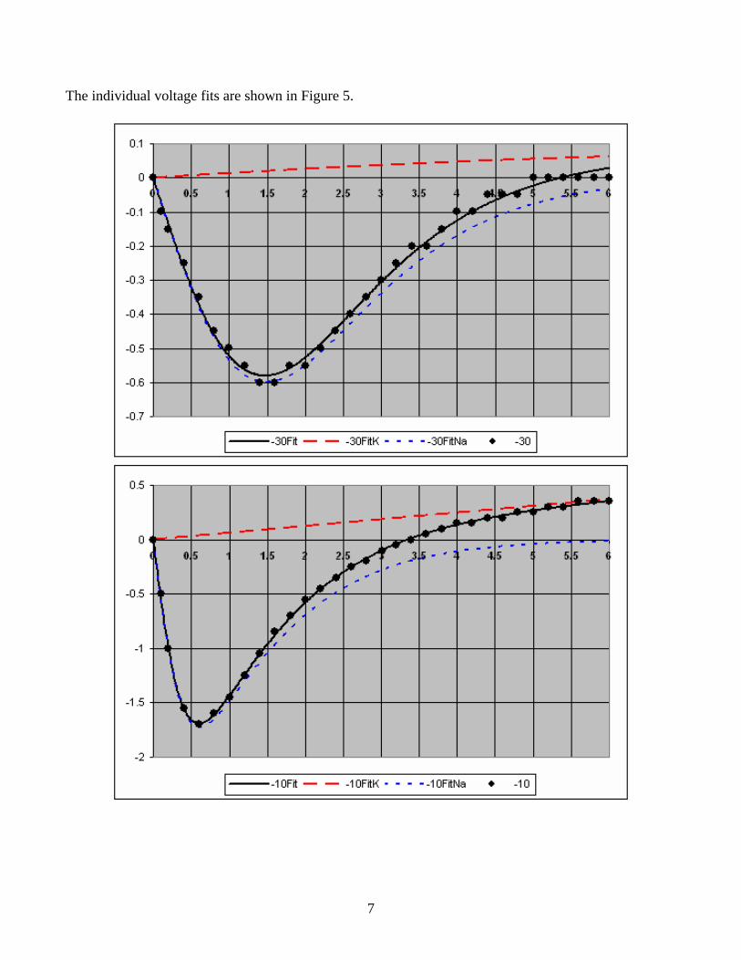
The individual voltage fits are shown in Figure 5.

8

9

10

Figure 5. Fits for each voltage showing the K and Na components.

This is a very good fit to the data.

11

The 35 fit parameters as a function of the clamping voltage are shown in Figure 6.

Figure 6. Fit parameters versus clamping voltage. The Nfactor ( NaJ ) scale is on the right.

However, Cronin (Cronin, 1987) points out that the fit parameters are more mathematically stable as a function of V if one factors ( )KV V− out of the potassium current and ( )NaV V− out of the sodium

current, where KV is the potassium Nernst potential ( )72 mV− and NaV is the sodium Nernst potential ( )55 mV+ , outside relative to inside. Then the equation for the current density is:

( ) ( ) ( ) ( ) ( ) ( )( ){ }( )

( )( ) ( ) ( )( )( ) ( ) ( )( )

( )

K

1 1 1 1Na

2 2 2 2

, tanh tanh

tanh tanh.

tanh tanh

K K K K K

Na N Na NNa

Na N Na N

J t V J V r V t V r V t t V V V

r V t r V t t VJ V V V

r V t r V t t V

⎡ ⎤= ⎡ ⎤ + − −⎣ ⎦ ⎣ ⎦

⎧ ⎫⎡ ⎤+ −⎡ ⎤⎣ ⎦⎪ ⎣ ⎦ ⎪+ −⎨ ⎬⎡ ⎤− − −⎡ ⎤⎪ ⎪⎣ ⎦ ⎣ ⎦⎩ ⎭

(1.3)

The voltage dependence of the parameters is indicated by, for example, ( )Kr V . The two hyperbolic-

tangent terms insure that the K and Na currents are zero at t = 0 and that the behavior at t = 0 can be exponential. (See Appendix 1.) This is a slight improvement over Eq. (1.2).

The “leakage current” is neglected because it is very small after about 0.05 milliseconds. (Malmivuo, 1995 Ch. 4.)

12

The values of the eight types of fit parameters for seven voltages are given in Table 4. Table 4. The 56 fit parameters at the different voltages in Eq. (1.3).

Potential -30 -10 10 30 50 70 90 ( )KJ V 0.01007 0.02634 0.02205 0.008366 0.01059 0.01033 0.01191 ( )

Kr V 4.8227 0.06417 0.2036 0.5917 0.6445 0.9015 0.8625 ( )

Kt V -14.54 -2.586 -0.1091 2.281 1.253 1.332 0.9236 ( )NaJ V 0.01587 0.04260 0.0229 0.02081 0.03455 0.01245 0.01107 ( )

N1r V 0.7900 2.463 7.708 17.61 14.66 34.53 33.06 ( )

N1t V 0.7645 0.01859 0.2254 0.1737 0.1272 0.08790 0.08545 ( )N2r V 0.4768 0.5217 0.6078 1.590 2.023 7.629 6.383 ( )

N2t V 1.366 -0.03291 0.8293 1.250 1.421 0.3978 0.4425 The 2χ of the least-squares fit is 0.0623 for fitting 224 data with 56 parameters. For those who might think that it easy to fit the 224 data with 56 parameters, I assure you that it is not easy! There are many local minima that must be negotiated around.

13

The 56 fit parameters as a function of the clamping voltage are shown in Figure 7.

Figure 7. Fit parameters versus clamping voltage. Right arrows indicate parameters for the right-hand scale.

These parameters as a function of voltage appear to be changing through several states.

14

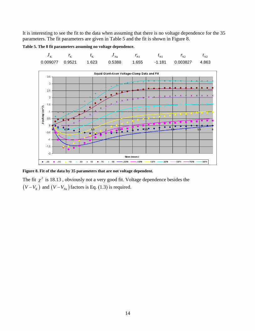
It is interesting to see the fit to the data when assuming that there is no voltage dependence for the 35 parameters. The fit parameters are given in Table 5 and the fit is shown in Figure 8. Table 5. The 8 fit parameters assuming no voltage dependence.

KJ Kr Kt NaJ N1r N1t N2r N2t 0.009077 0.9521 1.623 0.5388 1.655 -1.181 0.003827 4.863

Figure 8. Fit of the data by 35 parameters that are not voltage dependent.

The fit 2χ is 18.13 , obviously not a very good fit. Voltage dependence besides the ( ) ( ) and K NaV V V V− − factors is Eq. (1.3) is required.

15

The voltage dependence of the five types of fit parameters shown in Figure 7 is intriguing. I fitted them very precisely with functions of the voltage by varying 80 parameters as given in Table 6.

Table 6. Voltage-dependent equations for the 80 parameters of Eq. (1.3).

( )KJ V ( ) ( ) ( )1 1 1 2 2 2 3 3 3 tanh tanh tanhK K K K K K K K K Ka b r V V b r V V b r V V+ − + − + −⎡ ⎤ ⎡ ⎤ ⎡ ⎤⎣ ⎦ ⎣ ⎦ ⎣ ⎦

(10 parameters)

( )Kr V ( ) ( )1 4 4 2 5 5 tanh tanhK K K K K K Kc d r V V d r V V+ − + −⎡ ⎤ ⎡ ⎤⎣ ⎦ ⎣ ⎦

(7 parameters)

( )Kt V ( ) ( ) ( )1 6 6 2 7 7 3 8 8 tanh tanh tanhK K K K K K K K K Ke f r V V f r V V f r V V+ − + − + −⎡ ⎤ ⎡ ⎤ ⎡ ⎤⎣ ⎦ ⎣ ⎦ ⎣ ⎦

(10 parameters)

( )NaJ V

( ) ( )( ) ( )

1 1 1 2 2 2

3 3 3 4 4 4

tanh tanh

tanh tanhN N N N N N N

N N N N N N

a b r V V b r V V

b r V V b r V V

+ − + −⎡ ⎤ ⎡ ⎤⎣ ⎦ ⎣ ⎦+ − + −⎡ ⎤ ⎡ ⎤⎣ ⎦ ⎣ ⎦

(13 parameters)

( )Na1r V ( ) ( )1 1 5 5 2 6 6tanh tanhN N N N N N Nc d r V V d r V V+ − + −⎡ ⎤ ⎡ ⎤⎣ ⎦ ⎣ ⎦ (7 parameters)

( )Na1t V ( ) ( ) ( )1 1 8 8 2 9 9 3 10 10 tanh tanh tanhN N N N N N N N N Ne f r V V f r V V f r V V+ − + − + −⎡ ⎤ ⎡ ⎤ ⎡ ⎤⎣ ⎦ ⎣ ⎦ ⎣ ⎦ (10 parameters)

( )2Nar V

( ) ( )( ) ( )

2 4 11 11 5 12 12

6 13 13 7 14 14

tanh tanh

tanh tanhN N N N N N N

N N N N N N

c d r V V d r V V

d r V V d r V V

+ − + −⎡ ⎤ ⎡ ⎤⎣ ⎦ ⎣ ⎦+ − + −⎡ ⎤ ⎡ ⎤⎣ ⎦ ⎣ ⎦

(13 parameters)

( )Na2t V ( ) ( ) ( )2 4 15 15 5 16 16 6 17 17 tanh tanh tanhN N N N N N N N N Ne f r V V f r V V f r V V+ − + − + −⎡ ⎤ ⎡ ⎤ ⎡ ⎤⎣ ⎦ ⎣ ⎦ ⎣ ⎦ (10 parameters)

There are 80 parameters to be varied to fit the data. I do not use the definition of voltage relative to the resting potential, as do Hodgkin and Huxley; it just changes the value of the transitions positions by the value of the resting voltage (-60 volts). The justification for using the hyperbolic-tangent function for the voltage dependence is that it is expected that the parameters (conductance magnitude, rate and voltage position) for either ion’s channels changes from one state to another as a function of voltage. There may be several states for a given molecular channel and/or there may be several different types of molecular channels for either ion. The parameters for turning on and off a state may be different.

16

Then I fitted the original data by varying the 80 parameters to yield the fit shown in Figure 9.

Figure 9. Fits to the voltage-clamp data by varying the 80 voltage-dependent parameters.

The voltage-dependent parameters of the fit are given in Table 7. Table 7. The 80 fit parameters at the different voltages in Eq. (1.3).

( )KJ V ( )Kr V ( )Kt V ( )NaJ V ( )Na1r V ( )Na1t V ( )2Nar V ( )Na2t V

constant -0.05893 2.796 -7.82364 0.007086 16.27088 0.350503 -12.7982 0.191159factor 0.072051 -2.17475 9.710384 0.016787 -0.308 0.217533 -2.16391

position -14.9982 -16.6294 -19.1752 -20 -20.6659 13.25256 -20.9945 rate 0.990829 1.183216 6.160041 1.000002 15.63307 2.261918 5.002539

factor -0.00352 0.2467 -64.8999 -0.00822 5.674422 0.089785 39.68266 16.7079 position 16.85913 30.10066 14.17109 5.001146 4.559753 4.015038 31.23317 6.025746

rate 0.041169 5.961977 0.00016 0.994869 0.072784 1.153543 8.07E-05 0.003605factor 0.024006 -0.00138 9.07012 -0.54873 4.642999 -2.93567

position 59.50218 50.1996 49.94043 51.33782 50.49887 53.56772rate 0.003186 1.005443 1.132738 0.003752 0.771553 0.032717

factor -11.58461 -0.00472 -18.4761 position 65.87749 66.15592 94.9168

rate 0.00056 0.082027 0.220465 The 2χ is 0.174 for fitting 224 data with 80 parameters. Note the several position parameters that have nearly the same value, marked with colors. Also, some of the rate parameters have nearly the same value. Later we will set some of them equal and redo the fit.

17

The parameters’ values are given above. This is an alternate time and voltage dependence parameterization of the squid giant-axon membrane excitability to the usual Hodgkin-Huxley parameterization that involves differential equations. (http://en.wikipedia.org/wiki/Hodgkin-huxley_model) Undoubtedly, to some approximation of the hyperbolic functions used it is the same as the Hodgkin-Huxley model. The fact that many of the parameters in Table 7 have very nearly the same value is an expected result because the same channels may be active for the different voltage-dependent parameters. One can eliminate 34 variable parameters by equating and eliminating some of the parameters, leaving only 46 variable parameters. A higher 2 0.284χ = occurs when this is done and all the parameters are re-fitted, still a reasonably good fit to the data. The equated parameters are shown by colors in Table 8. Table 8. Voltage-dependent fit parameters after 34 parameters are eliminated, leaving 46 variable parameters. The colors indicate those of the original 50 parameters that have been equalized in the fit.

( )KJ V ( )

Kr V ( )Kt V ( )

NaJ V ( )Na1r V ( )

Na1t V ( )2Nar V ( )

Na2t V

constant -0.06459 2.585 -8.036 0.03753 19.80 0.4600 -20.05 -0.5831 factor 0.07731 -2.005 9.348 0.02750 -0.4777 -1.318

position -20.99 -20.99 -20.99 -20.99 -20.99 -20.99 rate 1.183 1.183 1.183 1.183 1.183 1.183

factor -0.002586 -0.04058 6.740 0.1583 -0.8756 18.83 position 9.189 9.189 9.189 9.189 9.189 9.189

rate 0.07463 2.519 0.07463 2.519 0.07463 0.003005 factor 14.84 37.89

position 29.70 29.70 rate 0.0004060 0.0004060

factor 0.1679 -0.03641 12.42 -7.252 3.266 -2.776 position 56.38 56.38 56.38 56.38 56.38 56.38

rate 0.0002238 0.03082 0.03082 0.0002228 0.03082 0.03082 factor -8.765 0.4245

position 66.57 66.57 rate 0.001572 0.001572

factor -23.90 position 95.17

rate 2.377 The fit to the data is shown in Figure 10.

18

Figure 10. The fit to the voltage-clamp data when 31 parameters are eliminated, leaving 49 parameters.

The equation now is:

( ) ( ) ( ), , ,K NaJ t V J t V J t V= + where

( ) ( ) ( ) ( ) ( ) ( )( ){ }( )K K, tanh tanhK K K K KJ t V J V r V t V r V t t V V V⎡ ⎤= ⎡ ⎤ + − −⎣ ⎦ ⎣ ⎦ and

( ) ( )( ) ( ) ( )( )( ) ( ) ( )( )

( )1 1 1 1Na Na

2 2 2 2

tanh tanh, .

tanh tanh

Na N Na NNa

Na N Na N

r V t r V t t VJ t V J V V V

r V t r V t t V

⎧ ⎫⎡ ⎤+ −⎡ ⎤⎣ ⎦⎪ ⎣ ⎦ ⎪= −⎨ ⎬⎡ ⎤− − −⎡ ⎤⎪ ⎪⎣ ⎦ ⎣ ⎦⎩ ⎭

19

The voltage-dependent parameters are

( ) ( )[ ]( )[ ] ( )[ ]

0.06459 0.07731tanh 1.183 20.99

0.002586 tanh 0.07463 9.189 0.1679tanh 0.0002238 56.38KJ V V

V V

= − + +

− − + −

( ) ( )[ ] ( )[ ]2.585 2.005 tanh 1.183 20.99 14.84 tanh 0.0004060 29.70Kr V V V= − + + −

( ) ( )[ ] ( )[ ]8.036 9.348 tanh 1.183 20.99 8.765 tanh 0.001572 66.57Kt V V V= − + + − −

( ) ( )[ ] ( )[ ]

( )[ ] ( )[ ]0.03753 0.02750 tanh 1.183 20.99 0.04058 tanh 2.519 9.189

0.03641tanh 0.03082 56.38 0.4245tanh 0.001572 66.57NaJ V V V

V V

= + + − −

− − + −

( ) ( )[ ] ( )[ ]1 19.80 6.740 tanh 0.07463 9.189 12.42tanh 0.03082 56.38Nar V V V= + − + −

( ) ( )[ ]

( )[ ] ( )[ ]1 0.4600 0.4777 tanh 1.183 20.99

0.1583tanh 2.519 9.189 7.252tanh 0.0002228 56.38Nat V V

V V

= − +

+ − − −

( ) ( )[ ] ( )[ ]

( )[ ] ( )[ ]2 20.05 0.8756 tanh 0.07463 9.189 37.89 tanh 0.0004060 29.70

+3.266tanh 0.03082 56.38 -23.90tanh 2.377 95.17Nat V V V

V V

= − − − + −

− −

( ) ( )[ ]

( )[ ] ( )[ ]2 0.5831 1.318 tanh 1.183 20.99

18.83tanh 0.003005 9.189 2.776tanh 0.03082 56.38Nat V V

V V

= − − +

+ − − −

20

The following graphs show the fit parameters as a function of voltage:

The transition centered at -20.99 volts is the most important one. The other two “transitions” at 9.189 volts and 56.38 volts are nearly linear behavior and are necessary for a good fit to the data. There appear to be three states negotiated by these three transitions. Perhaps only two transitions would do the job reasonably well.

The transition centered at -20.99 volts is the most important one. The other “transition” at 29.70 volts is just linear behavior and is necessary for a good fit to the data. There appear to be three states negotiated by these two transitions.

21

The transition centered at -20.99 volts is the most important one. The other “transition” at 66.57 volts is just linear behavior and is necessary for a good fit to the data. There appear to be three states negotiated by these two transitions.

The two transitions centered at -20.99 volts and 9.189 volts are the most important ones. The other two transitions at 56.38 volts and 66.57 volts are necessary for a good fit to the data. There appear to be five states negotiated by these four transitions, although four states and three transitions might do the job reasonably well.

22

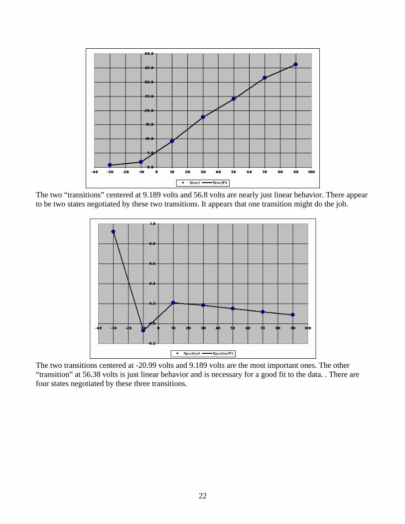
The two “transitions” centered at 9.189 volts and 56.8 volts are nearly just linear behavior. There appear to be two states negotiated by these two transitions. It appears that one transition might do the job.

The two transitions centered at -20.99 volts and 9.189 volts are the most important ones. The other “transition” at 56.38 volts is just linear behavior and is necessary for a good fit to the data. . There are four states negotiated by these three transitions.

23

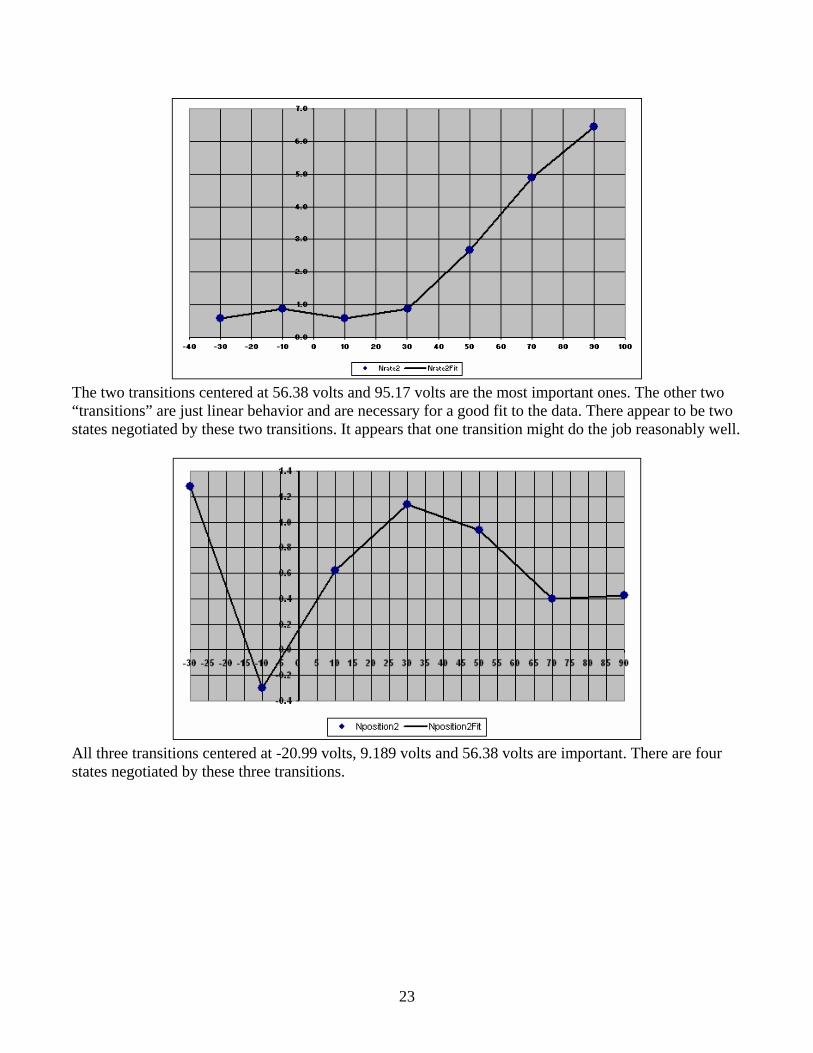
The two transitions centered at 56.38 volts and 95.17 volts are the most important ones. The other two “transitions” are just linear behavior and are necessary for a good fit to the data. There appear to be two states negotiated by these two transitions. It appears that one transition might do the job reasonably well.

All three transitions centered at -20.99 volts, 9.189 volts and 56.38 volts are important. There are four states negotiated by these three transitions.

24

However, note that many of the rates [ ( )nr V ] are quite small. For small argument [ ( ) / 2r x p π− < ] the

hyperbolic tangent, ( )tanh r x p⎡ ⎤−⎣ ⎦ , is well approximated by a straight line with slope r and intercept

p . That is, ( ) ( )tanh r x p r x p⎡ ⎤− ≅ −⎣ ⎦ . Using this in the parameters equations and refitting the data

yields a somewhat better fit ( 2 0.240χ = ) with the following parameters:

( ) ( )[ ]( )[ ] ( )[ ]

0.06441 0.07750 tanh 1.183 20.99

0.002964 tanh 0.07708 9.189 0.1220 0.0002234 56.80KJ V V

V V

= − + +

− − + −

( ) ( )[ ] ( )[ ]2.571 2.006 tanh 1.183 20.99 14.95 0.0004569 29.71Kr V V V= − + + −

( ) ( )[ ] ( )[ ]8.030 9.351tanh 1.183 20.99 8.772 0.001486 66.57Kt V V V= − + + − −

( ) ( )[ ] ( )[ ]

( )[ ] ( )[ ]0.04564 0.04638 tanh 1.183 20.99 0.07066 tanh 2.806 9.189

0.02672tanh 0.03430 56.80 0.3064 0.001486 66.57NaJ V V V

V V

= + + − −

− − + −

( ) ( )[ ] ( )[ ]1 19.41 6.581tanh 0.07708 9.189 12.23tanh 0.03430 56.80Nar V V V= + − + −

( ) ( )[ ]

( )[ ] ( )[ ]1 0.4392 0.5448 tanh 1.183 20.99

0.2266 tanh 2.806 9.189 7.645 0.0002834 56.80Nat V V

V V

= − +

+ − − −

( ) ( )[ ] ( )[ ]

( )[ ] ( )[ ]2 20.97 0.8032 tanh 0.07708 9.189 37.98 0.0004569 29.71

+2.741tanh 0.03430 56.80 -24.53tanh 2.377 95.17Nat V V V

V V

= − − − + −

− −

( ) ( )[ ]( )[ ] ( )[ ]

2 0.6134 1.297 tanh 1.183 20.99

18.96 0.002990 9.189 2.6531tanh 0.03430 56.80Nat V V

V V

= − − +

+ − − −

25

The voltage-dependent parameters are as shown in the following graphs:

The arrows pointing toward the right for some curves indicate that the scale is on the right.

26

27

Appendix 1: Hyperbolic Tangent The hyperbolic tangent’s definition (http://en.wikipedia.org/wiki/Hyperbolic_tangent) is

( )121tanhx⎡ ⎤+⎣ ⎦

( )tanh tanh .x xx x

e ee ex x −

−−+= = (1.4)

(e is the irrational number 2.71828183…. See http://en.wikipedia.org/wiki/Exponential_function.) Figure 11 is a graph of the hyperbolic tangent.

Figure 11. The hyperbolic-tangent function.

28

The hyperbolic-tangent has interesting asymptotic properties:

( )2

0 1

02

0 1 1

11

0

1

tanh .

xx

xx xx x x

xx

x

e ee e

e

ex

→−∞

> −−− →

< +

→+∞

⎧ ⎯⎯⎯⎯→⎪⎪⎯⎯⎯⎯→⎪− ⎯⎯⎯→⎨+⎪⎯⎯⎯⎯→ −⎪

⎪ ⎯⎯⎯⎯→⎩

−−

+

= (1.5)

Figure 12 shows the hyperbolic tangent and the ( )2 1xe − function plotted together.

Figure 12. The hyperbolic-tangent function and the exp( ) 1x − function.

29

So we see that the following holds:

( )21

1 21

0 221

1 2

12

1

0

1 tanh .

xx

xx

x x xx

x

x

ee e

e

ex

→−∞

−

− →

→ +

→+∞

⎧ ⎯⎯⎯⎯→⎪⎪ ⎯⎯⎯⎯→⎪⎪⎡ ⎤ ⎯⎯⎯→⎨+⎢ ⎥⎣ ⎦ ⎪⎯⎯⎯⎯→⎪

⎪ ⎯⎯⎯⎯→⎪⎩ +

+ = (1.6)

This function is graphed in Figure 13.

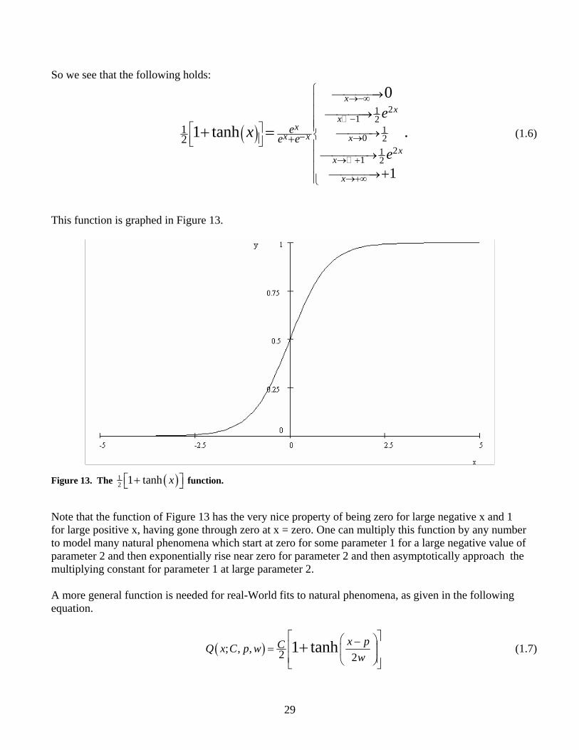
Figure 13. The ( )12 1 tanh x⎡ ⎤+⎣ ⎦ function.

Note that the function of Figure 13 has the very nice property of being zero for large negative x and 1 for large positive x, having gone through zero at x = zero. One can multiply this function by any number to model many natural phenomena which start at zero for some parameter 1 for a large negative value of parameter 2 and then exponentially rise near zero for parameter 2 and then asymptotically approach the multiplying constant for parameter 1 at large parameter 2. A more general function is needed for real-World fits to natural phenomena, as given in the following equation.

( ); , , 2 21 tanh x pCQ x C p w

w

⎡ ⎤⎛ ⎞−⎢ ⎥= ⎜ ⎟⎢ ⎥⎝ ⎠⎣ ⎦+ (1.7)

30

For example, 212 5

1 tanh x⎡ ⎤⎛ ⎞−⎢ ⎥⎜ ⎟⎢ ⎥⎝ ⎠⎣ ⎦+ is plotted in Figure 14.

Figure 14. Plot of21

25

1 tanh x −⎡ ⎤⎛ ⎞⎢ ⎥⎜ ⎟

⎝ ⎠⎣ ⎦+ .

We see why the parameter symbols w and p were chosen in the more general hyperbolic tangent in Eq. (1.3) when we take the derivative of the function.

( )2 ; , , .2 42 21 tanh 1 tanhd x p x pC C P x C p wwdx w w

⎧ ⎫⎡ ⎤ ⎡ ⎤⎛ ⎞ ⎛ ⎞− −⎪ ⎪⎢ ⎥ ⎢ ⎥= =⎜ ⎟ ⎜ ⎟⎨ ⎬⎢ ⎥ ⎢ ⎥⎝ ⎠ ⎝ ⎠⎪ ⎪⎣ ⎦ ⎣ ⎦⎩ ⎭+ − (1.8)

Figure 15 is a plot of 2 212 5 5

1 tanh x⎡ ⎤⎛ ⎞−⎢ ⎥⎜ ⎟⎢ ⎥⎝ ⎠⎣ ⎦− .

31

Figure 15. Plot of 2 212 5

51 tanh x −⎡ ⎤⎛ ⎞⎢ ⎥⎜ ⎟

⎝ ⎠⎣ ⎦− .

We see that the equation’s parameters have the following meanings:

peak position of the function. a measure of the width of the function; also the exponential time constant near .

height of the function.4

pw x pCw

== =

=

(1.9)

Sometimes natural data are in the form of an asymptotic curve such as Eq. (1.4) and sometimes natural data are in the form of a peaked curve, such as Eq. (1.5). As shown above, they are related by a calculus derivative, or inversely a calculus integral.

32

The hyperbolic tangent can be zero at x = 0 and have an exponential growth toward y near x = 0 or an exponential growth toward x near y = 0 as follows:

2 2tanh tanhp x p

w w−⎛ ⎞ ⎛ ⎞

⎜ ⎟ ⎜ ⎟⎝ ⎠ ⎝ ⎠

+ .

Examples:

2 22 2

tanh tanh x −⎛ ⎞ ⎛ ⎞⎜ ⎟ ⎜ ⎟⎝ ⎠ ⎝ ⎠

+ for exponential growth in y as a function of x:

Figure 16. Plot of2 22 2

tanh tanh x −⎛ ⎞ ⎛ ⎞⎜ ⎟ ⎜ ⎟⎝ ⎠ ⎝ ⎠

+ .

33

2 22 2

tanh tanh x− +⎛ ⎞ ⎛ ⎞⎜ ⎟ ⎜ ⎟⎝ ⎠ ⎝ ⎠

+ for exponential growth in x as a function of y:

Figure 17. Plot of 2 2

2 2tanh tanh x− +⎛ ⎞ ⎛ ⎞

⎜ ⎟ ⎜ ⎟⎝ ⎠ ⎝ ⎠

+ .

The expansion of the hyperbolic tangent for small argument is

(http://en.wikipedia.org/wiki/Hyperbolic_tangent)

So, ( ) ( ) ( ) 31

3tanh r x p r x p r x p⎡ ⎤ ⎡ ⎤− = − − − +⎣ ⎦ ⎣ ⎦ L for small x.

34

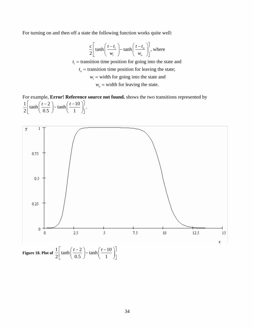
For turning on and then off a state the following function works quite well:

tanh tanh , where2

transition time position for going into the state andtransition time position for leaving the state; width for going into the state and

width

i o

i o

i

o

i

o

t t t tcw w

tt

ww

⎡ ⎤⎛ ⎞ ⎛ ⎞− −−⎢ ⎥⎜ ⎟ ⎜ ⎟

⎝ ⎠ ⎝ ⎠⎣ ⎦=

==

= for leaving the state.

For example, Error! Reference source not found. shows the two transitions represented by 1 2 10tanh tanh2 0.5 1

t t⎡ − − ⎤⎛ ⎞ ⎛ ⎞−⎜ ⎟ ⎜ ⎟⎢ ⎥⎝ ⎠ ⎝ ⎠⎣ ⎦.

Figure 18. Plot of 1 2 10tanh tanh2 0.5 1

t t⎡ − − ⎤⎛ ⎞ ⎛ ⎞−⎜ ⎟ ⎜ ⎟⎢ ⎥⎝ ⎠ ⎝ ⎠⎣ ⎦

35

Appendix 2: Hodgkin-Huxley Model

References Cronin, 1987: Mathematical Aspects of Hodgkin-Huxley Neural Theory, Jane Cronin, Cambridge University Press, 1987. Hille, 1984: Ionic Channels of Excitable Membranes, Bertil Hille, Sinauer Assoc. Inc, 1984. Malmivuo, 1995: Bioelectromagnetism: Principles and Applications of Bioelectric and Biomagnetic Fields, Jaakko Malmivuo and Robert Plonsey, Oxford Univ. Press,1995.