Embed Size (px)
Citation preview

Chapter 1
Systems of Linear Equations
1.1 Intro. to systems of linear equations
Main points in this section:
1. Definition of Linear system of equations and homogeneous systems.
2. Row-echelon form of a linear system and Gaussian elimination.
3. Solving linear system of equations using Gaussian elimination.
1
2 CHAPTER 1. SYSTEMS OF LINEAR EQUATIONS
Definition 1.1.1. A linear equation in n (unknown) variables x1, . . . , xn hasthe form
a1x1 + a2x2 + · · ·+ anxn = b.
Here a1, a2, . . . , an, b are real numbers. We say b is the constant term and aiis the coefficient of xi.
For real numbers s1, . . . , sn, if
a1s1 + a2s2 + · · ·+ ansn = b
we say thatx1 = s1, x2 = s2, . . . , xn = sn
is a solution of this equation.
1. An example of a linear equation in two unknowns is 2x + 7y = 5. Asolution of this equation is x = −1, y = 1. The equation has many moresolutions. The graph of this equation is a line.
2. An example of a linear equation in three unknowns is 2x+ y+ πz = π.
A solution of this equation is x = 0, y = 0, z = 1. The equation hasmany more solutions. The graph of this equation (in 3-space) isa plane.
1.1. INTRO. TO SYSTEMS OF LINEAR EQUATIONS 3
Definition 1.1.2. By a System of Linear Equations in n variables x1, x2, . . . , xnwe mean a collection of linear equations in these variables. A system of mlinear equations in these n variables can be written as
a11x1 + a12x2 + a13x3 + · · ·+ a1nxn = b1
a21x1 + a22x2 + a23x3 + · · ·+ a2nxn = b2
a31x1 + a32x2 + a33x3 + · · ·+ a3nxn = b3
· · ·· · ·am1x1 + am2x2 + am3x3 + · · ·+ amnxn = bm
where aij and bi are all real numbers.
Such a linear system is called a homogeneous linear system if
b1 = b2 = · · · = bm = 0.
1. A solution to such a system is a sequence of n numbers s1, . . . , sn thatis solution to all these m equations.
2. In two variables, here is an example of a system of two equation:{2x+ y = 3
x− 9y = −8
Clearly, x = 1, y = 1 is the (only) solution to this system.
Geometrically, solution given by precisely the point where the graphs(two lines) of these two equations meet.
Also note that the system {2x+ y = 3
2x+ y = 7
does not have any solution. Such a system would be called aninconsistent system. Geometrically, these two equations in the systemrepresent two parallel lines (they never meet).
4 CHAPTER 1. SYSTEMS OF LINEAR EQUATIONS
3. In three variables, the following is an example of a system of two equa-tion: {
2x+ y + 2z = 3
x− 9y + 2z = −8
Clearly, x = 1, y = 1, z = 0 is a solution to this system. This systemhas many more solutions. For example,
x = 11, y = 0, z = −19/2
is also a solution of this system. Geometrically, solution given by pre-cisely the points where the graphs (two planes) in 3-space of these twoequations meet.
4. Classification of linear systems: Given a linear system in n vari-ables, precisely one the the following three is true:
(a) The system has NO solution (inconsistent system).
(b) The system has exactly one solution (consistent system).
(c) The system has infinitely many solutions (consistent system).
5. Two systems of linear equations are called equivalent,if they have precisely the same set of solutions.
6. Following operations on a system produces an equivalent system:
(a) Interchange two equations.
(b) Multiply an equation by a nonzero constant.
(c) Add a multiple of an equation to another one.
These three operations are sometimes known asbasic or elementary operations.
1.1. INTRO. TO SYSTEMS OF LINEAR EQUATIONS 5
7. A linear system of the form
x1 + a12x2 + a13x3 + · · ·+ a1nxn = b1
x2 + a23x3 + · · ·+ a2nxn = b2
x3 + · · ·+ a3nxn = b3
· · ·· · ·
is said to be in row-echelon form. The point is:
(a) you drop one variable in each successive equation (step),
(b) The coefficient of the "leading variable" in equation is 1.
In two variables x, y this would (sometime) look like{x+ a12y = b1
y = b2
In three variables x, y, z this would (sometime) look likex+ a12y + a13z = b1
y + a23z = b2
z = b3
Theorem 1.1.3. The following are some facts:
1. Any system of linear equations is equivalent to a linear system in row-echelon form.
2. This can be achieved by a sequence of application of the three basicelementary operation described in (6).
3. This process is known as Gaussian elimination.
6 CHAPTER 1. SYSTEMS OF LINEAR EQUATIONS
Exercise 1.1.4. Reduce the following system row echelon form and solve:{x− 5y = 3 Eqn− 1
−8x+ 40y = 14 Eqn− 2
Add 8 times Enq-1 to Eqn-2:{x− 5y = 3 Eqn− 1
0 = 34 Eqn− 3
The Eqn-3 is absurd. So, the system has no solution. The system is incon-sistent.
Exercise 1.1.5. Reduce the following system to row echelon form and solve:{9x− 4y = 5 Eqn− 1
3x+ 2y = 0 Eqn− 2
Multiply Eqn-2 by 3: {9x− 4y = 5 Eqn− 1
9x+ 6y = 0 Eqn− 3
Subtract Eqn-1 from the Eqn-3{9x− 4y = 5 Eqn− 1
10y = −5 Eqn− 4
Divide Eqn-4 by 10: {9x− 4y = 5 Eqn− 1
y = −12
Eqn− 5
Divide Eqn-1 by 9: {x− 4
9y = 5
9Eqn− 6
y = −12
Eqn− 5

1.1. INTRO. TO SYSTEMS OF LINEAR EQUATIONS 7
This is the row-echelon form. Now substitute y = −12in Eqn-6
x− 4
9
(−1
2
)=
5
9or x =
1
3.
So, the solution isx =
1
3, y = −1
2.
Exercise 1.1.6. {x1+34
+ x2−13
= 1 Eqn− 1
x1 − x2
2= 6 Eqn− 2
multiply Eqn-1 by 12, Eqn-2 by 2 and simplify:{3x1 + 4x2 = 7 Eqn− 3
2x1 − x2 = 12 Eqn− 2
Add −23times Eqn-3 to Eqn-2:{
3x1 + 4x2 = 7 Eqn− 3−113x2 =
223
Eqn− 4
Multiply Eqn-4 by −311:{
3x1 + 4x2 = 7 Eqn− 3
x2 = −2 Eqn− 5
Multiply Eqn-3 by 13: {
x1 +43x2 =
73
Eqn− 6
x2 = −2 Eqn− 5
So, above is the row-echelon form of the system. Now substitute x2 = −2 inEqn-6 and get x1 = 8
3+ 7
3= 5. So, the systme is consistentand has unique
solutionx1 = 5, x2 = −2.

8 CHAPTER 1. SYSTEMS OF LINEAR EQUATIONS
Exercise 1.1.7. Deduce an equivalent row-echelon form and solve the fol-lowing system:
2x1 + 4x2 − x3 = 7 Eqn− 1
x1 − 11x2 + 4x3 = 3 Eqn− 2
10x1 − 6x2 + 4x3 = 3 Eqn− 3
First, switch Eqn-1 and Eqn-2:x1 − 11x2 + 4x3 = 3 Eqn− 2
2x1 + 4x2 − x3 = 7 Eqn− 1
10x1 − 6x2 + 4x3 = 3 Eqn− 3
Subtract 2 times Eqn-2 from Eqn-1 and 10 times Eqn-2 from Eqn-3:x1 − 11x2 + 4x3 = 3 Eqn− 2
26x2 − 9x3 = 1 Eqn− 4
104x2 − 36x3 = −27 Eqn− 5
Subtract 4 times Eqn-4 from Eqn-5:x1 − 11x2 + 4x3 = 3 Eqn− 2
26x2 − 9x3 = 1 Eqn− 4
0 = −31 Eqn− 6
The system is inconsistent because Eqn-6 is absurd. To obtain the row-echelon form, we divid Eqn-4 by 26:
x1 − 11x2 + 4x3 = 3 Eqn− 3
x2 − 926x3 =
126
Eqn− 7
0 = −31 Eqn− 6
1.1. INTRO. TO SYSTEMS OF LINEAR EQUATIONS 9
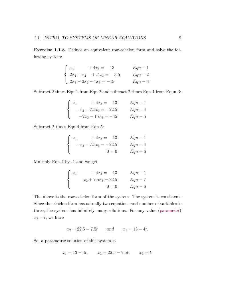
Exercise 1.1.8. Deduce an equivalent row-echelon form and solve the fol-lowing system:
x1 + 4x3 = 13 Eqn− 1
2x1 − x2 + .5x3 = 3.5 Eqn− 2
2x1 − 2x2 − 7x3 = −19 Eqn− 3
Subtract 2 times Eqn-1 from Eqn-2 and subtract 2 times Eqn-1 from Equn-3:x1 + 4x3 = 13 Eqn− 1
−x2 − 7.5x3 = −22.5 Eqn− 4
−2x2 − 15x3 = −45 Eqn− 5
Subtract 2 times Eqn-4 from Eqn-5:x1 + 4x3 = 13 Eqn− 1
−x2 − 7.5x3 = −22.5 Eqn− 4
0 = 0 Eqn− 6
Multiply Eqn-4 by -1 and we getx1 + 4x3 = 13 Eqn− 1
x2 + 7.5x3 = 22.5 Eqn− 7
0 = 0 Eqn− 6
The above is the row-echelon form of the system. The system is consistent.Since the echelon form has actually two equations and number of variables isthree, the system has infinitely many solutions. For any value (parameter)x3 = t, we have
x2 = 22.5− 7.5t and x1 = 13− 4t.
So, a parametric solution of this system is
x1 = 13− 4t, x2 = 22.5− 7.5t, x3 = t.
10 CHAPTER 1. SYSTEMS OF LINEAR EQUATIONS
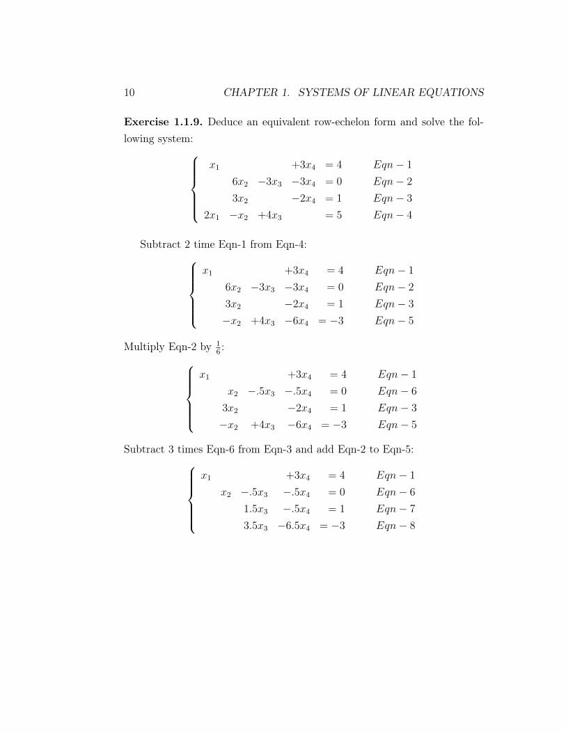
Exercise 1.1.9. Deduce an equivalent row-echelon form and solve the fol-lowing system:
x1 +3x4 = 4 Eqn− 1
6x2 −3x3 −3x4 = 0 Eqn− 2
3x2 −2x4 = 1 Eqn− 3
2x1 −x2 +4x3 = 5 Eqn− 4
Subtract 2 time Eqn-1 from Eqn-4:x1 +3x4 = 4 Eqn− 1
6x2 −3x3 −3x4 = 0 Eqn− 2
3x2 −2x4 = 1 Eqn− 3
−x2 +4x3 −6x4 = −3 Eqn− 5
Multiply Eqn-2 by 16:
x1 +3x4 = 4 Eqn− 1
x2 −.5x3 −.5x4 = 0 Eqn− 6
3x2 −2x4 = 1 Eqn− 3
−x2 +4x3 −6x4 = −3 Eqn− 5
Subtract 3 times Eqn-6 from Eqn-3 and add Eqn-2 to Eqn-5:x1 +3x4 = 4 Eqn− 1
x2 −.5x3 −.5x4 = 0 Eqn− 6
1.5x3 −.5x4 = 1 Eqn− 7
3.5x3 −6.5x4 = −3 Eqn− 8

1.1. INTRO. TO SYSTEMS OF LINEAR EQUATIONS 11
Multiply Eqn-7 by 23:
x1 +3x4 = 4 Eqn− 1
x2 −.5x3 −.5x4 = 0 Eqn− 6
x3 −13x4 = 2
3Eqn− 9
3.5x3 −6.5x4 = −3 Eqn− 8
Subtract 3.5 times Eqn-9 from Eqn-8:x1 +3x4 = 4 Eqn− 1
x2 −.5x3 −.5x4 = 0 Eqn− 6
x3 −13x4 = 2
3Eqn− 9
−163x4 = −16
3Eqn− 10
Multiply Eqn-10 by − 316:
x1 +3x4 = 4 Eqn− 1
x2 −.5x3 −.5x4 = 0 Eqn− 6
x3 −13x4 = 2
3Eqn− 9
x4 = 1 Eqn− 11
The above is a row-echelon form of the system. By back-substitution:
x4 = 1, x3 =2
3+
1
3= 1, x2 = 1, x1 = 1.
12 CHAPTER 1. SYSTEMS OF LINEAR EQUATIONS
1.2 Gaussian, Gauss-Jordan Elimination
Main points in this section:
1. Definition of matrices.
2. Elementary row operation on a matrix.
3. Definition of Row-echelon form of matrix.
4. Gaussian and Gauss-Jordan elimination.
5. Solving sytems of linear equations using Gaussian elimination and Gauss-Jordan elimination.
1.2. GAUSSIAN, GAUSS-JORDAN ELIMINATION 13
Definition 1.2.1. For two positive integers m,n and m × n−matrix is arectangular array
a11 a12 a13 · · · a1n
a21 a22 a23 · · · a2n
a31 a32 a33 · · · a3n
· · · · · · · · · · · · · · ·· · · · · · · · · · · · · · ·am1 am2 am3 · · · amn
1. the array has m rows ana n column.
2. Here aij is a real number, to be called ijth−entry. This entry sits inthe ith−row jth−column. The first subscript i of aij is called the rowsubscript and j is called the column subscript.
3. It is possible to talk about matrices whose entries aij are not real num-bers. We can talk about matrices of any kind of objects. For example,we can consider matrices complex numbers. However, in this course,we consider matrices with real entries ONLY, and such matrices arealso called real matrices.
4. We say that the size of the above matrix is m× n.
5. A square matrix of order n is a matrix whose number of rows andcolumns are same and equal to n.
6. For a square matrix of order n, the entries a11, a22, . . . , ann are calledthe main diaginal entries.

14 CHAPTER 1. SYSTEMS OF LINEAR EQUATIONS
The most common use, for this class, of matrices is to represent systemof liner equation. Given a system of liner equations, an associated matrixto be called the augmented matrix contains all the information regardingthe system.
Definition 1.2.2. Given a system of m linear equations
a11x1 + a12x2 + a13x3 + · · ·+ a1nxn = b1
a21x1 + a22x2 + a23x3 + · · ·+ a2nxn = b2
a31x1 + a32x2 + a33x3 + · · ·+ a3nxn = b3
· · · · · · · · · · · ·am1x1 + am2x2 + am3x3 + · · ·+ amnxn = bm
the augmented matrix of the system is defined as
a11 a12 a13 · · · a1n b1
a21 a22 a23 · · · a2n b2
a31 a32 a33 · · · a3n b3
· · · · · · · · · · · · · · · · · ·am1 am2 am3 · · · amn bm
and the coefficient matrix is defined as
a11 a12 a13 · · · a1n
a21 a22 a23 · · · a2n
a31 a32 a33 · · · a3n
· · · · · · · · · · · · · · ·am1 am2 am3 · · · amn
.
1. Conversely, given a m× (n+1) matrix, we can write down a system oflinear m equations in n unknowns (variables).
2. Consider the linear system (from exercise 1.1.4):{x− 5y = 3
−8x+ 40y = 14
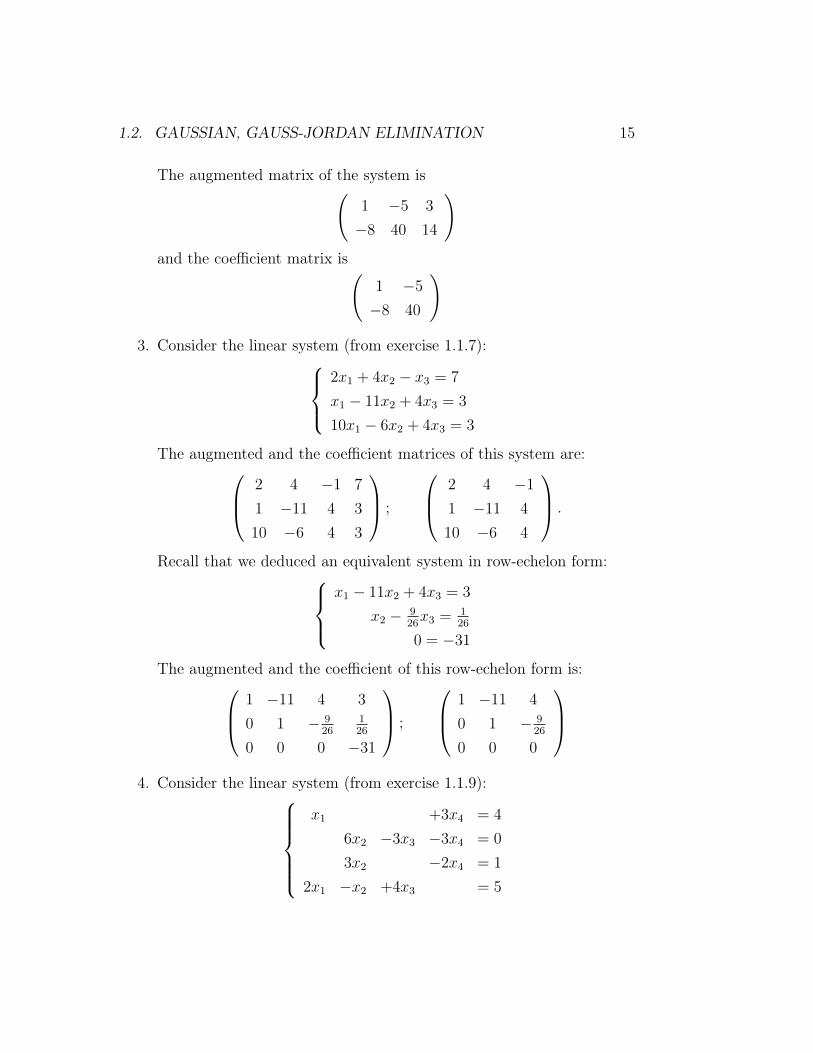
1.2. GAUSSIAN, GAUSS-JORDAN ELIMINATION 15
The augmented matrix of the system is(1 −5 3
−8 40 14
)and the coefficient matrix is(
1 −5−8 40
)
3. Consider the linear system (from exercise 1.1.7):2x1 + 4x2 − x3 = 7
x1 − 11x2 + 4x3 = 3
10x1 − 6x2 + 4x3 = 3
The augmented and the coefficient matrices of this system are: 2 4 −1 7
1 −11 4 3
10 −6 4 3
;
2 4 −11 −11 4
10 −6 4
.
Recall that we deduced an equivalent system in row-echelon form:x1 − 11x2 + 4x3 = 3
x2 − 926x3 =
126
0 = −31
The augmented and the coefficient of this row-echelon form is: 1 −11 4 3
0 1 − 926
126
0 0 0 −31
;
1 −11 4
0 1 − 926
0 0 0
4. Consider the linear system (from exercise 1.1.9):
x1 +3x4 = 4
6x2 −3x3 −3x4 = 0
3x2 −2x4 = 1
2x1 −x2 +4x3 = 5
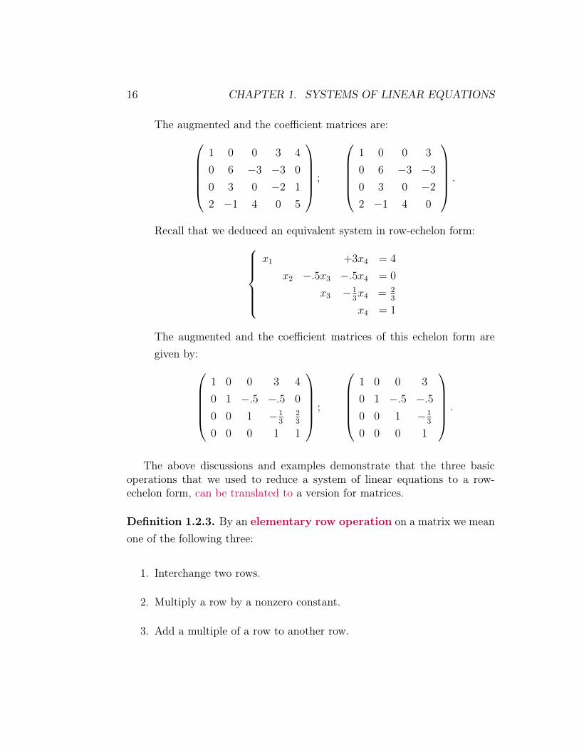
16 CHAPTER 1. SYSTEMS OF LINEAR EQUATIONS
The augmented and the coefficient matrices are:1 0 0 3 4
0 6 −3 −3 0
0 3 0 −2 1
2 −1 4 0 5
;
1 0 0 3
0 6 −3 −30 3 0 −22 −1 4 0
.
Recall that we deduced an equivalent system in row-echelon form:x1 +3x4 = 4
x2 −.5x3 −.5x4 = 0
x3 −13x4 = 2
3
x4 = 1
The augmented and the coefficient matrices of this echelon form aregiven by:
1 0 0 3 4
0 1 −.5 −.5 0
0 0 1 −13
23
0 0 0 1 1
;
1 0 0 3
0 1 −.5 −.50 0 1 −1
3
0 0 0 1
.
The above discussions and examples demonstrate that the three basicoperations that we used to reduce a system of linear equations to a row-echelon form, can be translated to a version for matrices.
Definition 1.2.3. By an elementary row operation on a matrix we meanone of the following three:
1. Interchange two rows.
2. Multiply a row by a nonzero constant.
3. Add a multiple of a row to another row.
1.2. GAUSSIAN, GAUSS-JORDAN ELIMINATION 17
Two matrices are said to be row-equivalent if one can be obtained fromanother by application of a sequence of elementary row operations. Tworow-equivalent matrices, correspond to two equivalent system of equations.
Now we define the matrix version of row-echelon form:
Definition 1.2.4. A matrix is said to be in row-echelon form, if it hasthe following properties:
1. All rows consisting entirely of zeros occur at the bottom of the matrix.
2. For each non-zero row, first nonzero entry is 1 (called the leading 1).
3. For each successive nonzero rows, the leading 1 in the higher row isfarther to the left than the leading 1 in the lower row.
A matrix in row-echelon form is said to be in reduced row-echelonform, if every column that has a leading 1 has zeros in evey position aboveand below the leading 1.
Theorem 1.2.5. Suppose M is a matrix. Then, M is
row-equivalent to a matrix B, which is in row-echelon
form. We gave (see below definition 1.2.2 above) the
augmented matrix of the system in exercise 1.1.9 and
that of the equivalent system in row-echelon form.

18 CHAPTER 1. SYSTEMS OF LINEAR EQUATIONS
Definition 1.2.6. Consider a system of linear equations, as in definition1.2.2. The method of solving this system by Gaussian elimination withback-substitution equation is described as follows:
1. Write the augmented matrix of the system.
2. Use the elemetary row operations to reduce the augmented matrix toa matrix in row-echelon form.
3. Write the linear system corresponding to the row-echeclon matrix andsolve by back-substitution.
Exercise 1.2.7 (Ex 1.1.9, use GE). We will use the method of Gaussianelimination with beck-substitution to solve exercise 1.1.9, using analogoussteps. Recall the system:
x1 +3x4 = 4 Eqn− 1
6x2 −3x3 −3x4 = 0 Eqn− 2
3x2 −2x4 = 1 Eqn− 3
2x1 −x2 +4x3 = 5 Eqn− 4
The augmented matrix is:1 0 0 3 4
0 6 −3 −3 0
0 3 0 −2 1
2 −1 4 0 5
Subtract 2 times row-1 from row-4:
1 0 0 3 4
0 6 −3 −3 0
0 3 0 −2 1
0 −1 4 −6 −3
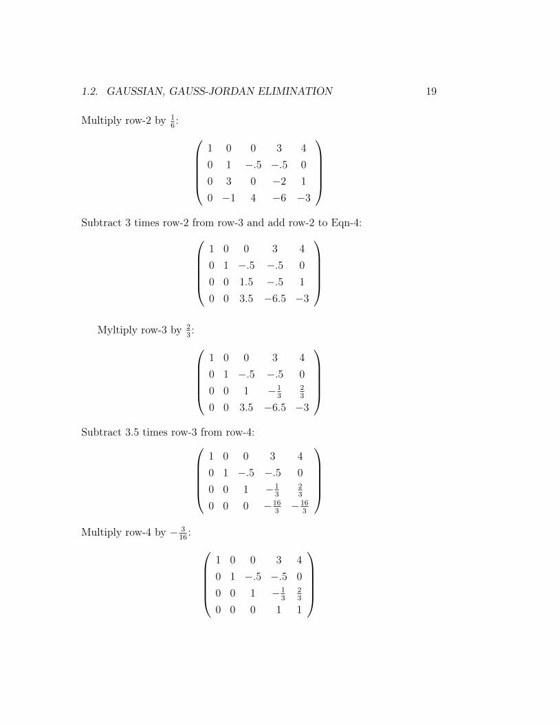
1.2. GAUSSIAN, GAUSS-JORDAN ELIMINATION 19
Multiply row-2 by 16:
1 0 0 3 4
0 1 −.5 −.5 0
0 3 0 −2 1
0 −1 4 −6 −3
Subtract 3 times row-2 from row-3 and add row-2 to Eqn-4:
1 0 0 3 4
0 1 −.5 −.5 0
0 0 1.5 −.5 1
0 0 3.5 −6.5 −3
Myltiply row-3 by 2
3:
1 0 0 3 4
0 1 −.5 −.5 0
0 0 1 −13
23
0 0 3.5 −6.5 −3
Subtract 3.5 times row-3 from row-4:
1 0 0 3 4
0 1 −.5 −.5 0
0 0 1 −13
23
0 0 0 −163−16
3
Multiply row-4 by − 3
16:
1 0 0 3 4
0 1 −.5 −.5 0
0 0 1 −13
23
0 0 0 1 1
20 CHAPTER 1. SYSTEMS OF LINEAR EQUATIONS
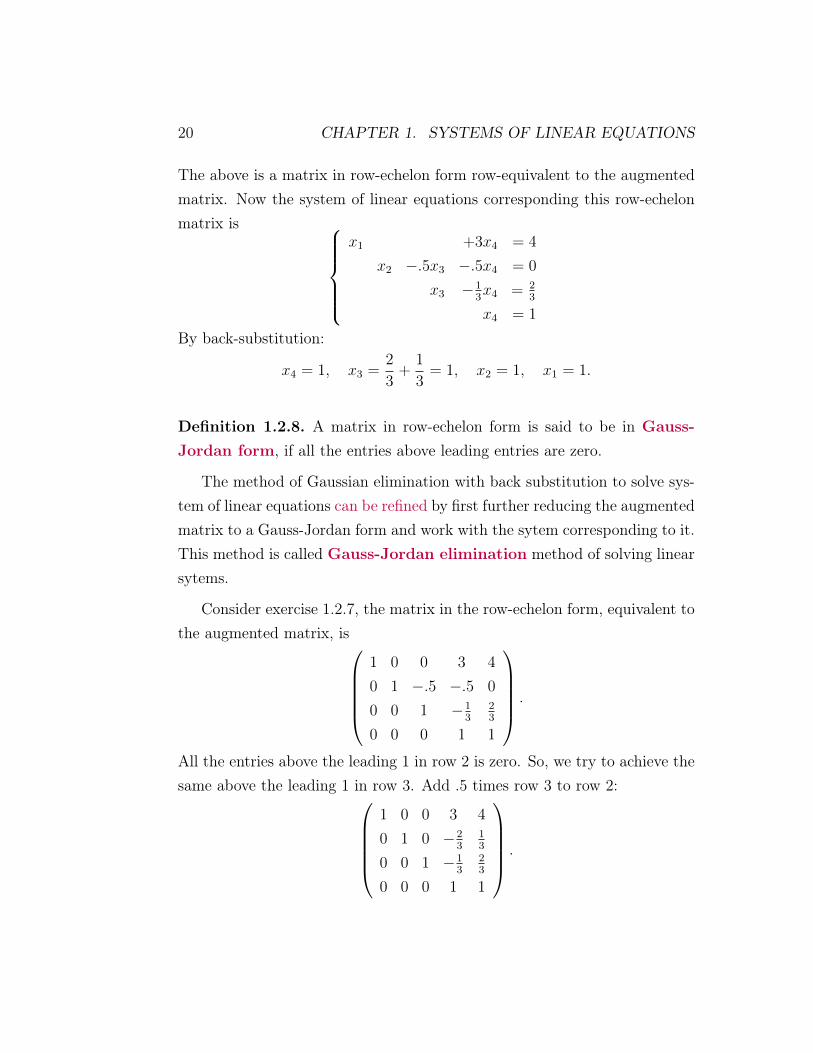
The above is a matrix in row-echelon form row-equivalent to the augmentedmatrix. Now the system of linear equations corresponding this row-echelonmatrix is
x1 +3x4 = 4
x2 −.5x3 −.5x4 = 0
x3 −13x4 = 2
3
x4 = 1
By back-substitution:
x4 = 1, x3 =2
3+
1
3= 1, x2 = 1, x1 = 1.
Definition 1.2.8. A matrix in row-echelon form is said to be in Gauss-Jordan form, if all the entries above leading entries are zero.
The method of Gaussian elimination with back substitution to solve sys-tem of linear equations can be refined by first further reducing the augmentedmatrix to a Gauss-Jordan form and work with the sytem corresponding to it.This method is called Gauss-Jordan elimination method of solving linearsytems.
Consider exercise 1.2.7, the matrix in the row-echelon form, equivalent tothe augmented matrix, is
1 0 0 3 4
0 1 −.5 −.5 0
0 0 1 −13
23
0 0 0 1 1
.
All the entries above the leading 1 in row 2 is zero. So, we try to achieve thesame above the leading 1 in row 3. Add .5 times row 3 to row 2:
1 0 0 3 4
0 1 0 −23
13
0 0 1 −13
23
0 0 0 1 1
.
1.2. GAUSSIAN, GAUSS-JORDAN ELIMINATION 21
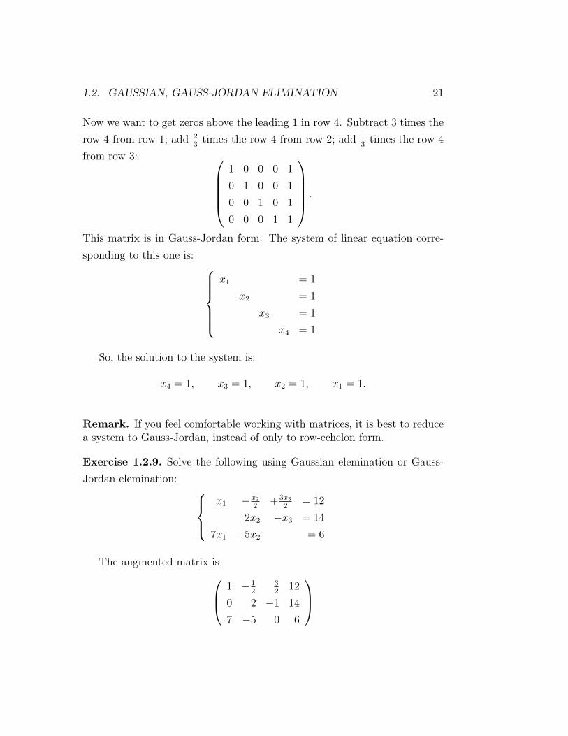
Now we want to get zeros above the leading 1 in row 4. Subtract 3 times therow 4 from row 1; add 2
3times the row 4 from row 2; add 1
3times the row 4
from row 3: 1 0 0 0 1
0 1 0 0 1
0 0 1 0 1
0 0 0 1 1
.
This matrix is in Gauss-Jordan form. The system of linear equation corre-sponding to this one is:
x1 = 1
x2 = 1
x3 = 1
x4 = 1
So, the solution to the system is:
x4 = 1, x3 = 1, x2 = 1, x1 = 1.
Remark. If you feel comfortable working with matrices, it is best to reducea system to Gauss-Jordan, instead of only to row-echelon form.
Exercise 1.2.9. Solve the following using Gaussian elemination or Gauss-Jordan elemination:
x1 −x2
2+3x3
2= 12
2x2 −x3 = 14
7x1 −5x2 = 6
The augmented matrix is 1 −12
32
12
0 2 −1 14
7 −5 0 6
22 CHAPTER 1. SYSTEMS OF LINEAR EQUATIONS
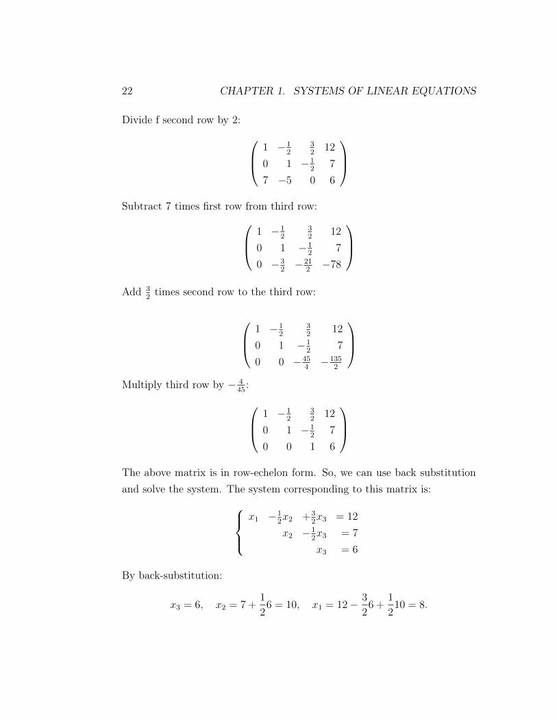
Divide f second row by 2: 1 −12
32
12
0 1 −12
7
7 −5 0 6
Subtract 7 times first row from third row: 1 −1
232
12
0 1 −12
7
0 −32−21
2−78
Add 3
2times second row to the third row:
1 −12
32
12
0 1 −12
7
0 0 −454−135
2
Multiply third row by − 4
45: 1 −1
232
12
0 1 −12
7
0 0 1 6
The above matrix is in row-echelon form. So, we can use back substitutionand solve the system. The system corresponding to this matrix is:
x1 −12x2 +3
2x3 = 12
x2 −12x3 = 7
x3 = 6
By back-substitution:
x3 = 6, x2 = 7 +1
26 = 10, x1 = 12− 3
26 +
1
210 = 8.

1.2. GAUSSIAN, GAUSS-JORDAN ELIMINATION 23
Alternately, we could reduce the row-echelon matrix 1 −12
32
12
0 1 −12
7
0 0 1 6
to a Gauss-Jordan form. We will do this. To do this add 1
2time the second
row to the first: 1 0 1.25 15.5
0 1 −12
7
0 0 1 6
Subtract 1.25 times third rwo from the first: 1 0 0 8
0 1 −12
7
0 0 1 6
Now add .5 time the third row to the second: 1 0 0 8
0 1 0 10
0 0 1 6
This matrix is in Gauss-Jordan form. The system of liner equations corre-sponding to this matrix is:
x1 = 8
x2 = 10
x3 = 6
This gives the solution of our system.
Exercise 1.2.10. Solve the following using Gaussian elemination or Gauss-Jordan elemination:
2x1 +3x3 = 3
4x1 −3x2 +7x3 = 5
6x1 −9x2 +12x3 = 7
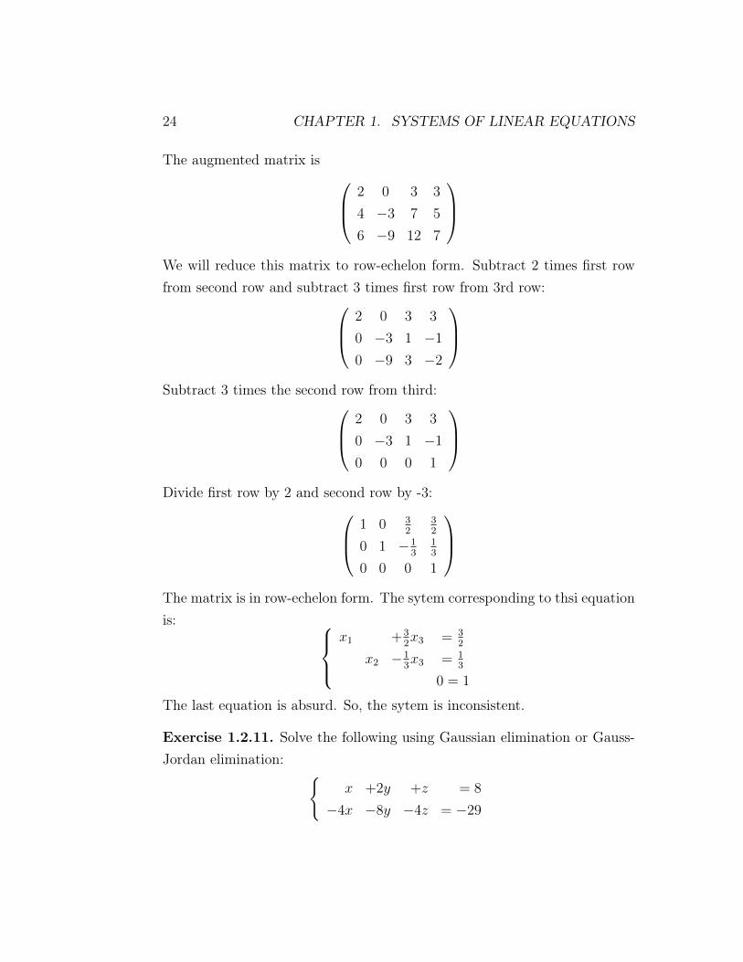
24 CHAPTER 1. SYSTEMS OF LINEAR EQUATIONS
The augmented matrix is 2 0 3 3
4 −3 7 5
6 −9 12 7
We will reduce this matrix to row-echelon form. Subtract 2 times first rowfrom second row and subtract 3 times first row from 3rd row: 2 0 3 3
0 −3 1 −10 −9 3 −2
Subtract 3 times the second row from third: 2 0 3 3
0 −3 1 −10 0 0 1
Divide first row by 2 and second row by -3: 1 0 3
232
0 1 −13
13
0 0 0 1
The matrix is in row-echelon form. The sytem corresponding to thsi equationis:
x1 +32x3 = 3
2
x2 −13x3 = 1
3
0 = 1
The last equation is absurd. So, the sytem is inconsistent.
Exercise 1.2.11. Solve the following using Gaussian elimination or Gauss-Jordan elimination: {
x +2y +z = 8
−4x −8y −4z = −29
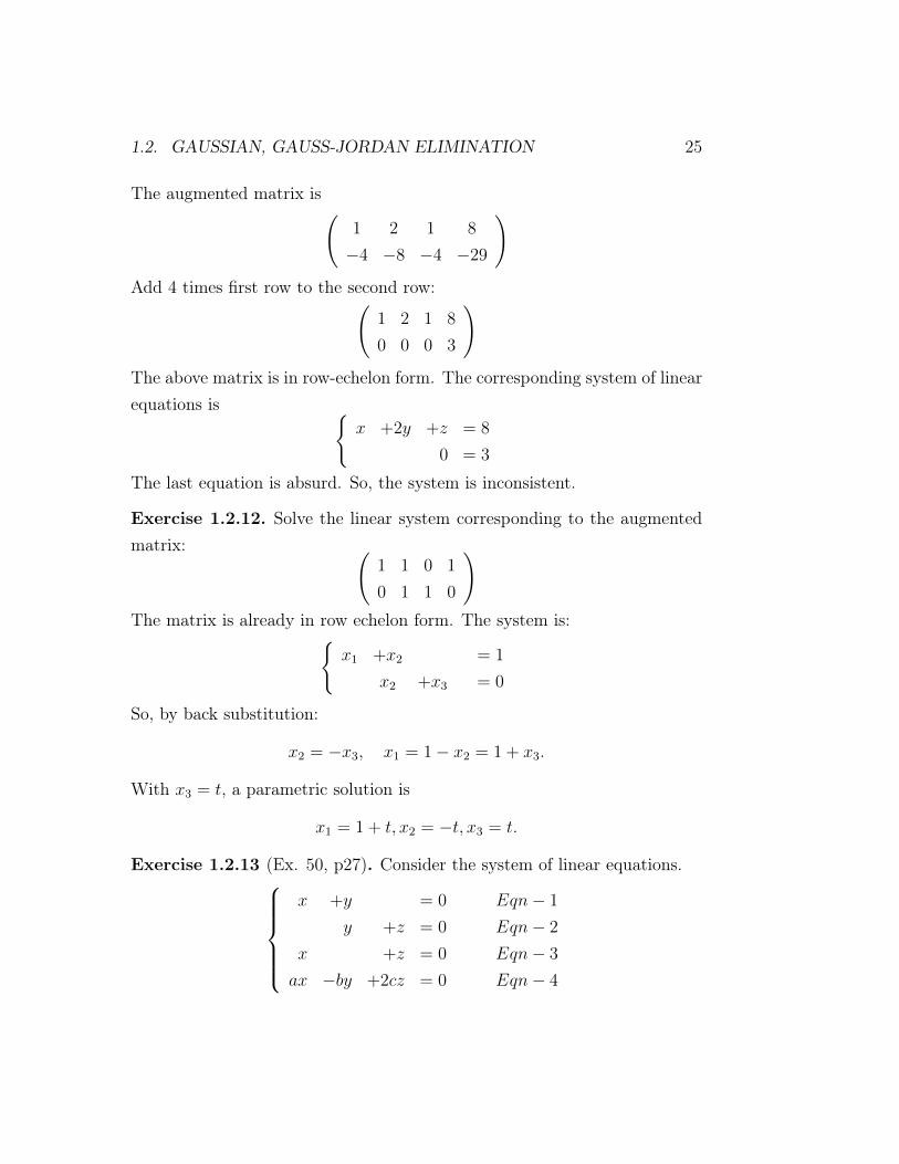
1.2. GAUSSIAN, GAUSS-JORDAN ELIMINATION 25
The augmented matrix is(1 2 1 8
−4 −8 −4 −29
)Add 4 times first row to the second row:(
1 2 1 8
0 0 0 3
)The above matrix is in row-echelon form. The corresponding system of linearequations is {
x +2y +z = 8
0 = 3
The last equation is absurd. So, the system is inconsistent.
Exercise 1.2.12. Solve the linear system corresponding to the augmentedmatrix: (
1 1 0 1
0 1 1 0
)The matrix is already in row echelon form. The system is:{
x1 +x2 = 1
x2 +x3 = 0
So, by back substitution:
x2 = −x3, x1 = 1− x2 = 1 + x3.
With x3 = t, a parametric solution is
x1 = 1 + t, x2 = −t, x3 = t.
Exercise 1.2.13 (Ex. 50, p27). Consider the system of linear equations.x +y = 0 Eqn− 1
y +z = 0 Eqn− 2
x +z = 0 Eqn− 3
ax −by +2cz = 0 Eqn− 4
26 CHAPTER 1. SYSTEMS OF LINEAR EQUATIONS
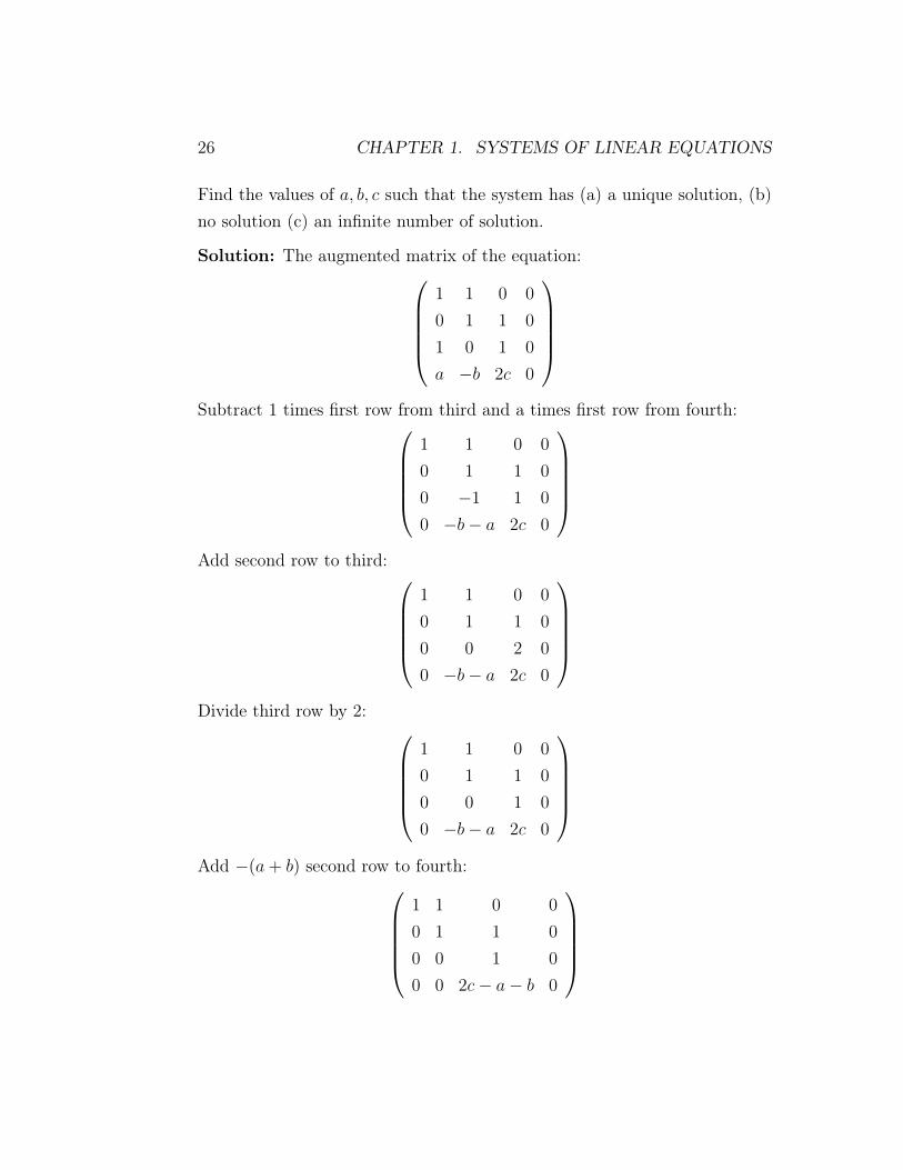
Find the values of a, b, c such that the system has (a) a unique solution, (b)no solution (c) an infinite number of solution.
Solution: The augmented matrix of the equation:1 1 0 0
0 1 1 0
1 0 1 0
a −b 2c 0
Subtract 1 times first row from third and a times first row from fourth:
1 1 0 0
0 1 1 0
0 −1 1 0
0 −b− a 2c 0
Add second row to third:
1 1 0 0
0 1 1 0
0 0 2 0
0 −b− a 2c 0
Divide third row by 2:
1 1 0 0
0 1 1 0
0 0 1 0
0 −b− a 2c 0
Add −(a+ b) second row to fourth:
1 1 0 0
0 1 1 0
0 0 1 0
0 0 2c− a− b 0

1.2. GAUSSIAN, GAUSS-JORDAN ELIMINATION 27
Subtract 2c− a− b times third row from fourth: i1 1 0 0
0 1 1 0
0 0 1 0
0 0 0 0
The matrix is in row-echelon form. The corresponding liner system is:
x +y = 0
y +z = 0
z = 0
0 = 0
The system is consistent for all values of a, b, c, and by back substitutionthe system has unique solution x = y = z = 0.

28 CHAPTER 1. SYSTEMS OF LINEAR EQUATIONS
1.3 Application of Linear systems
(Read Only, for now)
We do a few applications of linear systems.
We do the following applications:
1. Fitting polynimials,
2. Network anlysis,
3. Kirchoff’s Laws for electrical networks
System of linear equations is much easier to handle than nonlinear sys-tems. (I do not mean for this class only, I mean for expert mathematiciansand scientists.) In fact, it is really very difficult to handle nonlinear systems.That is why, there is a wide range of applications of linear systems.
1.3.1 Polynomial curve fitting
Recall the facts:
1. there is exactly one line y = c + mx that passes through two givenpoints;
2. there is exactly one parabola y = ax2+bx+c that passes through threegiven points (barring some exceptions).
3. More generally, given n number of points in the plane and there isexactly one polynomials p(x) of degree n − 1, so that the graph ofy = p(x) will pass through these n points We describe it as follows.
1.3. APPLICATION OF LINEAR SYSTEMS 29
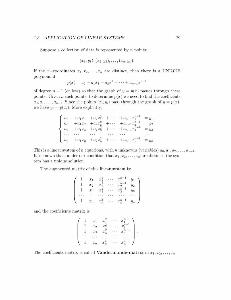
Suppose a collection of data is represented by n points:
(x1, y1), (x2, y2), . . . , (xn, yn).
If the x−coordinates x1, x2, . . . , xn are distinct, then there is a UNIQUEpolynomial
p(x) = a0 + a1x1 + a2x2 + · · ·+ an−1x
n−1
of degree n− 1 (or less) so that the graph of y = p(x) passes through thesepoints. Given n such points, to determine p(x) we need to find the coefficentsa0, a1, . . . , an−1. Since the points (xi, yi) pass through the graph of y = p(x),we have yi = p(xi). More explicitly,
a0 +a1x1 +a2x21 + · · · +an−1x
n−11 = y1
a0 +a1x2 +a2x22 + · · · +an−1x
n−12 = y2
a0 +a1x3 +a2x23 + · · · +an−1x
n−13 = y3
· · · · · · · · · · · · · · · · · ·a0 +a1xn +a2x
2n + · · · +an−1x
n−1n = yn
This is a linear system of n equations, with n unknowns (variables) a0, a1, a2, . . . , an−1.It is known that, under our condition that x1, x2, . . . , xn are distinct, the sys-tem has a unique solution.
The augmented matrix of this linear system is:1 x1 x21 · · · xn−1
1 y11 x2 x22 · · · xn−1
2 y21 x3 x23 · · · xn−1
3 y3· · · · · · · · · · · · · · · · · ·1 xn x2n · · · xn−1
n yn
and the coefficients matrix is
1 x1 x21 · · · xn−11
1 x2 x22 · · · xn−12
1 x3 x23 · · · xn−13
· · · · · · · · · · · · · · ·1 xn x2n · · · xn−1
n
.
The coefficients matrix is called Vandermonde-matrix in x1, x2, . . . , xn.

30 CHAPTER 1. SYSTEMS OF LINEAR EQUATIONS
Exercise 1.3.1. Determine the polynomial function (of degree 2) that passesthrough the points (2, 4), (3, 6), (4, 10).
Solution: Let p(x) = a+bx+cx2. Since these points pass through the graphof y = p(x) = a+ bx+ cx2, we have
a +b2 +c22 = 4
a +b3 +c32 = 6
a +b4 +c42 = 10
or
a +2b +4c = 4
a +3b +9c = 6
a +4b +16c = 10
The augmented matrix of this system is: 1 2 4 4
1 3 9 6
1 4 16 10
Now we reduce the matrix to the row-echelon form. To do this subtract row-1from row-2 and row-3: 1 2 4 4
0 1 5 2
0 2 12 6
Now, subtract 2 times row-2 from row-3: 1 2 4 4
0 1 5 2
0 0 2 2
Divide the last row by 2: 1 2 4 4
0 1 5 2
0 0 1 1
The matrix is in row-echelon form. They linear system corresponding to thismatrix is:
a +2b +4c = 4
b +5c = 2
c = 1.

1.3. APPLICATION OF LINEAR SYSTEMS 31
By back substitution
c = 1, b = 2− 5 = −3, a = 4− 4 + 6 = 6
So p(x) = a+ bx+ cx2 = 6− 3x+ x2. Use your TI to graph it.
Exercise 1.3.2. Some US census population data is given in the followingtable.
Y ear 1980 1990 2000
population y 227 249 281
Here population is given in millions.
1. Fit a second degree polynomial passing through these points.
2. Use it to predict popolation in year 2010 abd 2020.
Solution: Let t be the variable time and set t = 0 for the year 1980. Thetable reduces to
t 0 10 20
y 227 249 281
Let p(t) = a+ bt+ ct2 be the polynomial that fits this data. Since the datapoints pass through the graph of y = p(t) = a+ bt+ ct2, we have
a +b0 +c02 = 227
a +b10 +c102 = 249
a +b20 +c202 = 281
or
a = 227
a +10b +100c = 249
a +20b +400c = 281
The augmented matrix is 1 0 0 227
1 10 100 249
1 20 400 281

32 CHAPTER 1. SYSTEMS OF LINEAR EQUATIONS
Now use TI-84 (or you can hand reduce) to reduce the matrix to Gauss-Jordan form: 1 0 0 227
0 1 0 1.7
0 0 1 .05
So,
a = 227, b = 1.7, c = 0.05 and y = p(t) = 227 + 1.7t+ .05t2.
This answers part (1). For part (2), for year 2010, wehave t = 30 andprediceted population is
p(30) = 227 + 1.7 ∗ 30 + .05 ∗ 302 = 323 mi.
Similarly, for year 2020, wehave t = 40 and prediceted population is
p(30) = 227 + 1.7 ∗ 40 + .05 ∗ 402 = 375 mi.
1.3.2 Network Analysis
A network consists of junctions and branches. Following is an example ofnetwrok:
x //Z
13 //
y
??
z
��
Such network systems are used to model diverse situations, including in eco-nomics, traffic, telephone signal and electrical engineering. Such models as-sumes, the total flow into a junction is equal to total flow out of thejunction. Accordingly, above network is represented by
x = y + 13 + z.

1.3. APPLICATION OF LINEAR SYSTEMS 33
Exercise 1.3.3. The flow of traffic through a network of telephone towersis shown in the following figure:
30 //A
x1 //
x2
��
B15 //
x4
��
20//Y x5
//
x3
??
Z 35//
1. Solve this system for x1, x2, x3, x4, x5.
2. Find the traffic flow when x2 = 20 and x3 = 5.
3. Find the traffic flow when x2 = 15 and x3 = 0.
Solution: From junction A, we get
x1 + x2 = 30
From junction B, we get
x1 + x3 = 15 + x4 OR x1 + x3 − x4 = 15
From junction Y, we get
x2 + 20 = x3 + x5 OR x2 − x3 − x5 = −20
From junction Z, we getx4 + x5 = 35.
We will write the system in a better way:x1 +x2 = 30
x1 +x3 −x4 = 15
x2 −x3 −x5 = −20x4 +x5 = 35

34 CHAPTER 1. SYSTEMS OF LINEAR EQUATIONS
To solve thsi linear system, we write the augmented matrix:1 1 0 0 0 30
1 0 1 −1 0 15
0 1 −1 0 −1 −200 0 0 1 1 35
We will reduce this matrix to row-echelon form. Subtract row 1 from row 2:
1 1 0 0 0 30
0 −1 1 −1 0 −150 1 −1 0 −1 −200 0 0 1 1 35
Add second row to third:
1 1 0 0 0 30
0 −1 1 −1 0 −150 0 0 −1 −1 −350 0 0 1 1 35
Add third roe to fourth:
1 1 0 0 0 30
0 −1 1 −1 0 −150 0 0 −1 −1 −350 0 0 0 0 0
Multiply second row by -1 and third row by -1:
1 1 0 0 0 30
0 1 −1 1 0 15
0 0 0 1 1 35
0 0 0 0 0 0

1.3. APPLICATION OF LINEAR SYSTEMS 35
The matrix is in row-echelon form. The corresponding linear system is givenby:
x1 +x2 = 30
x2 −x3 +x4 = 15
x4 +x5 = 35
0 = 0
Parametrically, with x2 = t, x3 = s, we have
x1 = 300−t, x2 = t, x3 = s, x4 = 15−t+s, x5 = 35−x4 = 150+t−s.
This answers (1). For (2) t = x2 = 20, s = x3 = 5. So,
x1 = 10, x2 = 20, x3 = 5, x4 = 0, x5 = 30.
For (3) t = x2 = 15, s = x3 = 0. So,
x1 = 15, x2 = 15, x3 = 0, x4 = 0, x5 = 35.
1.3.3 Kirchhoff’s Laws
Similarly, system of Linear equations is also applicable in electrical network.Analysis of electrical network is guided by two properties known as Kirch-hoff’s Laws:
1. All the current flowing into a junction must flow out of it.
2. The sum of the products IR (I is current and R is resistance) arounda closed path is equal to the total voltage.
A battery is denoted by |` or a| and the resistance is denoted by.

36 CHAPTER 1. SYSTEMS OF LINEAR EQUATIONS
Exercise 1.3.4. Consider the electrical circuit.
��
I1
R1=4
3 v
|`oo
J1I2
R2=3//J2
OO
��
\\
I3
R3=1
1 v
|`oo
(The circuit should be connected, I could not draw a better one.) Use Kirchhoff-Law to determine I1, I2, I3.
Solution: Apply (1) of Kirchhoff-Law to junction J1, we have
I1 +I3 = I2 Eqn− 1
Applying the same to J2 wil give the same equation. So, we will not write it.
Now apply (2) of Kirchhoff-Law{R1I1 +R2I2 = 3
R2I2 +R3I3 = 1OR
{4I1 +3I2 = 3 Eqn− 2
3I2 +I3 = 1 Eqn− 3
The the network system is given byI1 −I2 +I3 = 0 Eqn− 1
4I1 +3I2 = 3 Eqn− 2
3I2 +I3 = 1 Eqn− 3
The augmented matrix is: 1 −1 1 0
4 3 0 3
0 3 1 1
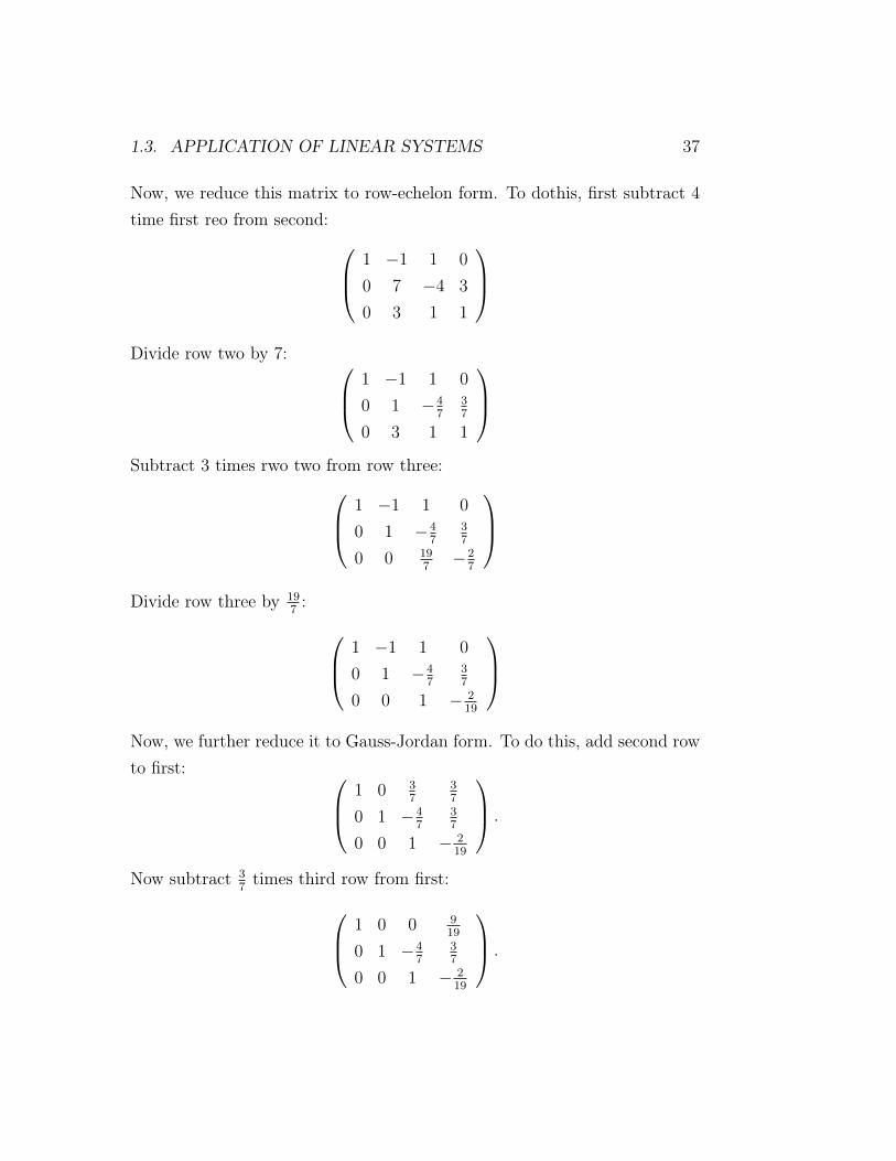
1.3. APPLICATION OF LINEAR SYSTEMS 37
Now, we reduce this matrix to row-echelon form. To dothis, first subtract 4time first reo from second: 1 −1 1 0
0 7 −4 3
0 3 1 1
Divide row two by 7: 1 −1 1 0
0 1 −47
37
0 3 1 1
Subtract 3 times rwo two from row three: 1 −1 1 0
0 1 −47
37
0 0 197−2
7
Divide row three by 19
7: 1 −1 1 0
0 1 −47
37
0 0 1 − 219
Now, we further reduce it to Gauss-Jordan form. To do this, add second rowto first: 1 0 3
737
0 1 −47
37
0 0 1 − 219
.
Now subtract 37times third row from first: 1 0 0 9
19
0 1 −47
37
0 0 1 − 219
.

38 CHAPTER 1. SYSTEMS OF LINEAR EQUATIONS
Now, add 47time third roe to second: 1 0 0 9
19
0 1 0 719
0 0 1 − 219
.
The corresponding linear system s given by,I1 = 9
19
I2 = 719
I3 = − 219

Bibliography
[Textbook] Ron Larson Elementary Linear Algebra, 7th Edition
39