1

Chapter 1: Introduction James W. Murray(10/01/01) Univ. Washington______________________________________________________________________

Chemical oceanography is the study of everything about the chemistry of theocean and is based on the distribution and dynamics of elements, isotopes, atoms andmolecules. This ranges from fundamental physical, thermodynamic and kinetic chemistryto two-way interactions of ocean chemistry with biological, geological and physicalprocesses. It encompasses both inorganic and organic chemistry. The cornerstones ofprogress are breakthroughs in analytical chemistry. If this definition seems broad considerthat the field also includes study of atmospheric and terrestrial (and some contendextraterrestrial) processes. If oceanography is a wagon wheel, chemical oceanography sitsat the middle, and is the most interdisciplinary of all the options.

Chemical oceanography includes processes that occur on a wide range of spatialand temporal scales; from global to regional to local to microscopic spatial dimensionsand time scales from geological epochs to glacial-interglacial to millennial, decadal,interannual, seasonal, diurnal and all the way to microsecond time scales (Fig. 1-1).

Fig. 1-1The advantages of the chemical perspective include:1. Hugh information potential due to the large number of elements (93), isotopes (260),

naturally occurring radioisotopes (78) and compounds (innumerable) present in theocean.

2. Chemical measurements have high representativeness, reproducibility andpredictability (statistically meaningful).

3. Quantitative treatments are possible (stoichiometries, balances, predictions of reactionrates and extents, age estimates, paleotemperatures). All the normal rules of chemistryapply.

4. Chemical changes indicate processes and integrate the net effect of multiple previousevents. This is important because most of the ocean is inaccessible to directobservation, and past environmental records are preserved in marine sediments.

2

How and why is this field relevant?

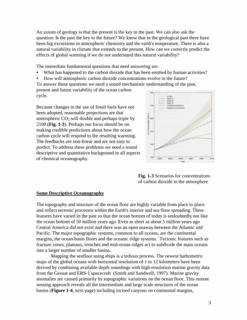
As the world enters the 21st century there will increased focus on cycling of carbon. Mostof chemical oceanography in one way or another can be related to carbon compounds andcarbon cycling and this is a worthy focus. We are all aware that CO2 and othergreenhouse gases are increasing in the atmosphere. There is no better example to showthan the classic data from C.D. Keeling (1976) showing the seasonal oscillations and thesteady annual increase of CO2 at the Mauna Loa Observatory (Fig. 1-2). Most expertsconclude we are already witnessing the impact of this increase as global warming and thesignal is expected to become increasingly more pronounced. Thus, an important focus ofan education in chemical oceanography should be on the concentrations of carbon speciesand their controlling mechanisms.

Fig. 1-2 Mauna Loa CO2

The ocean carbon cycle influences atmospheric CO2 via changes in the net air-sea CO2

flux that are driven by differences in the partial pressure of CO2, PCO2 , between thesurface ocean and atmosphere. The inventory of dissolved CO2 in the oceans is 50-60times greater than that in the atmosphere, so a small perturbation of the ocean carboncycle can result in a substantial change in the concentration of CO2 in the atmosphere.The regional and vertical partitioning of carbon in the ocean is dominated by twointerdependent carbon pumps that deplete the surface ocean of total CO2 relative to deepwater. Because the solubility of CO2 increases with decreasing temperature, theSOLUBILITY PUMP transfers CO2 to the deep sea during formation of cold deep waterat high latitudes. This is a link of the ocean carbon cycle to physical processes. At thesame time the BIOLOGICAL PUMP removes carbon from surface waters by settling oforganic and inorganic carbon derived from biological production. The biological pumptransports organic carbon and CaCO3 to deeper water where much if it is dissolved orremineralized increasing the total CO2 reservoir in the deep sea that is isolated from theatmosphere. This is a link of the ocean carbon cycle to biological processes.

3

An axiom of geology is that the present is the key to the past. We can also ask thequestion: Is the past the key to the future? We know that in the geological past there havebeen big excursions in atmospheric chemistry and the earth's temperature. There is also anatural variability in climate that extends to the present. How can we correctly predict theeffects of global warming if we do not understand this natural variability?

The immediate fundamental questions that need answering are:• What has happened to the carbon dioxide that has been emitted by human activities?• How will atmospheric carbon dioxide concentrations evolve in the future?To answer these questions we need a sound mechanistic understanding of the past,present and future variability of the ocean carboncycle.

Because changes in the use of fossil fuels have notbeen adopted, reasonable projections are thatatmospheric CO2 will double and perhaps triple by2100 (Fig. 1-3). Perhaps our focus should be onmaking credible predictions about how the oceancarbon cycle will respond to the resulting warming.The feedbacks are non-linear and are not easy topredict. To address these problems we need a sounddescriptive and quantitative background in all aspectsof chemical oceanography.

Fig. 1-3 Scenarios for concentrationsof carbon dioxide in the atmosphere

Some Descriptive Oceanography

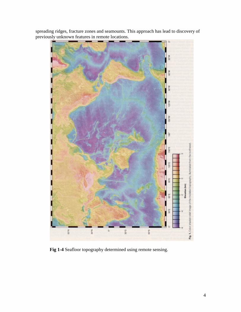
The topography and structure of the ocean floor are highly variable from place to placeand reflect tectonic processes within the Earth's interior and sea floor spreading. Thesefeatures have varied in the past so that the ocean bottom of today is undoubtedly not likethe ocean bottom of 50 million years ago. Even as short as about 5 million years agoCentral America did not exist and there was an open seaway between the Atlantic andPacific. The major topographic systems, common to all oceans, are the continentalmargins, the ocean-basin floors and the oceanic ridge systems. Tectonic features such asfracture zones, plateaus, trenches and mid-ocean ridges act to subdivide the main oceansinto a larger number of smaller basins.

Mapping the seafloor using ships is a tedious process. The newest bathometricmaps of the global oceans with horizontal resolution of 1 to 12 kilometers have beenderived by combining available depth soundings with high-resolution marine gravity datafrom the Geosat and ERS-1 spacecraft (Smith and Sandwell, 1997). Marine gravityanomalies are caused primarily by topographic variations on the ocean floor. This remotesensing approach reveals all the intermediate and large scale structures of the oceanbasins (Figure 1-4, next page) including incised canyons on continental margins,

4

spreading ridges, fracture zones and seamounts. This approach has lead to discovery ofpreviously unknown features in remote locations.

Fig 1-4 Seafloor topography determined using remote sensing.

5

The continental margin regions are the transition zones between the continentsand ocean basins. The major features at ocean margins are shown schematically in Fig. 1-5. Though the features may vary, the general features shown occur in all ocean basins inthe form of either two sequences: shelf-slope-rise-basin or shelf-slope-trench-basin.

Fig 1-5 Schematic Diagram of Continental Margins

The continental shelf is the submerged continuation of the adjacent land, modifiedin part by marine erosion or sediment deposition. The seaward edge of the continentalshelf can frequently be clearly seen and it is called the shelf break. The shelf break tendsto occur at a depth of about 200 m over most of the ocean. Sea level was almost 125mlower during Pleistocene glacial maxima. At those times the shoreline was close to theedge of present continental shelf, which was then a coastal plain. On average, thecontinental shelf is about 70 km wide, although it can vary widely (compare the east coastof China with the west coast of Peru). The Arctic Ocean has the largest proportion ofshelf to total area of all the world’s oceans.

The continental slope is characterized as the region where the gradient of thetopography changes from 1:1000 on the shelf to greater than 1:40. Thus continentalslopes are the relatively narrow, steeply inclined submerged edges of the continents. Thecontinental slope may form one side of an ocean trench as it does off the west coast ofMexico or Peru or it may grade into the continental rise as it does off the east coast of theU.S. The ocean trenches are the topographic reflection of the subduction of oceanicplates beneath the continents. The greatest ocean depths occur in such trenches. Thedeepest is the Challenger Deep which descends to 11,035 meters in the Marianas Trench.The continental rises are mainly depositional features that are the result of coalescing ofthick wedges of sedimentary deposits carried by turbidity currents down the slope andalong the margin by boundary currents. Deposition is caused by the reduction in currentspeed when it flows out onto the gently sloping rise. Gradually the continental rise gradesinto the ocean basins and the abyssal plains.

One of the great accomplishments of the plate tectonics revolution was therecognition that we live on a dynamic planet. The interaction of ocean crustal processes

6

with the ocean itself takes place through the cycling of sea water through the crust. Aschematic drawing of the solid Earth's plate tectonic cycle is shown in Fig. 1-6. The threemajor tectonic components are plate creation at mid-ocean spreading centers,modification of the plate as it traverses the mantle, and subduction of the plate andcreation of new crust at the convergent margins.

Fig. 1-6

The relationships between ocean depths and land elevations are shown in Fig. 1-6.On the average the continents are 840 m above sea level while the average depth of theoceans is 3730 m. If the earth were a smooth sphere with the land planed off to fill theocean basins the earth would be uniformly covered by water to a depth of 2430 m.

Fig. 1-6 Frequency of land elevations and ocean depths

7

The area, volume and average depth of the ocean basins and some marginal seas are givenin Table 1-1.

Table 1-1

The Pacific Ocean is the largest and contains more than one-half of the Earth's water. Italso receives the least river water per area of the major oceans (Table 1-2).

Table 1-2

Paradoxically it is also the least salty (Table 1-3). The land area of the entire Earth isstrongly skewed toward the northern hemisphere.

Table 1-3 Average temperature and salinity of different oceans.

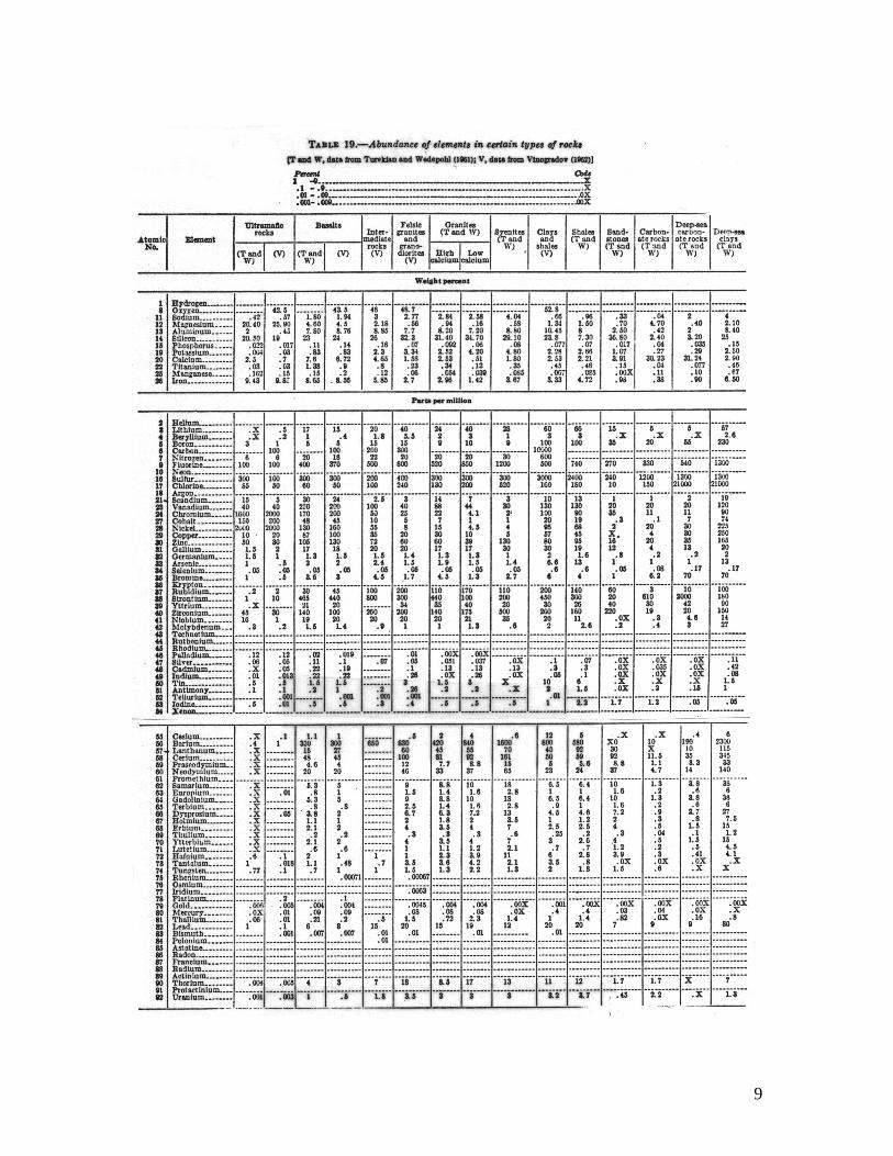
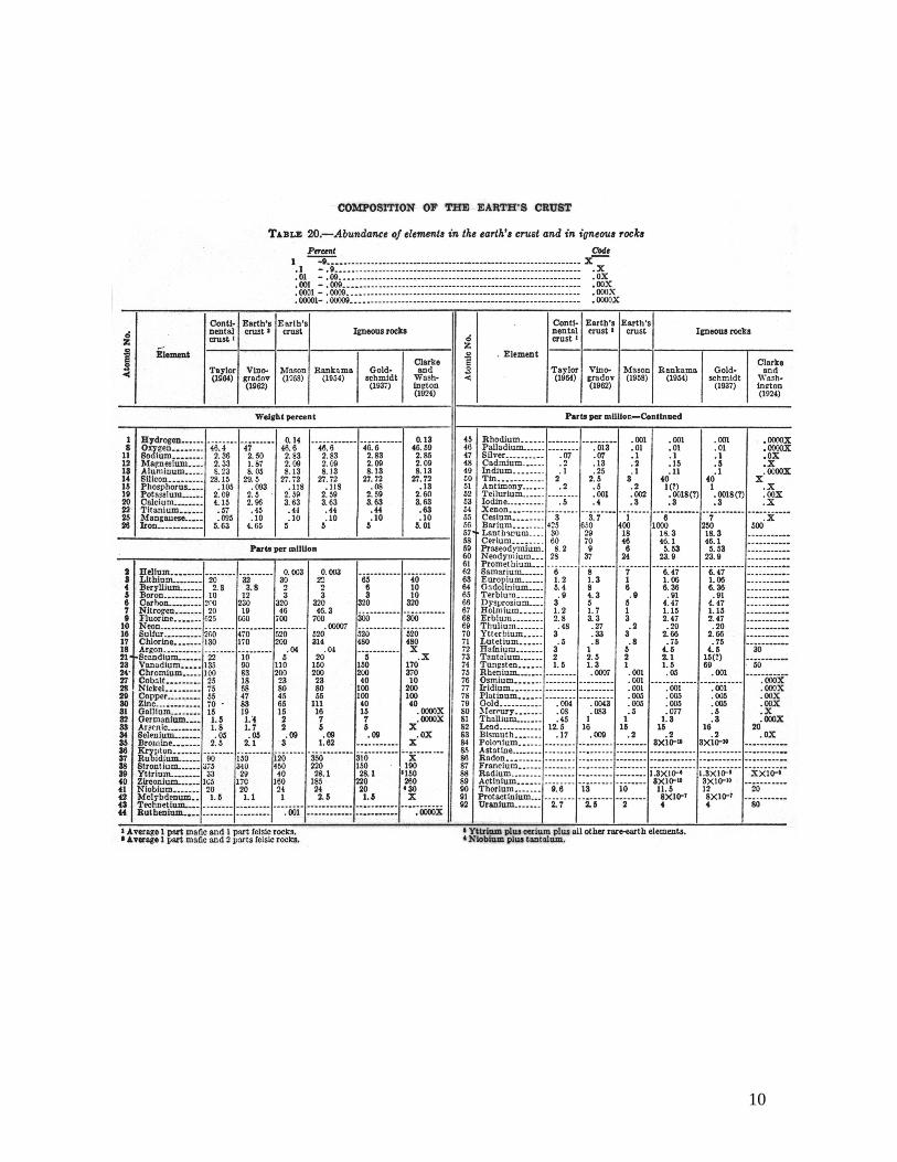
Average compositions of the crust and different rock types

The average composition of different types of rocks and the earth's crust is givenin Table 1-4 and Table 1-5, respectively (from Parker, 1967) . These rocks are frequently

8

used for comparison or reference in geochemical studies thus it is useful to have thesetables available.

9

10

11

Global Water CycleWater is present on Earth in three phases - solid, liquid and gas. The ocean

contains the bulk (97%) of the earth's water (1.37 x 109 km3 or about 1.37 x 1024 g) andmoderates the global water cycle. Glaciers are the second largest reservoir with about 2%of the total. The distribution of the mass of water, is about 80% in the ocean and about20% as pore water in sediments and sedimentary rocks. The reservoir of water in rivers,lakes and the atmosphere is a trivial part of the total (0.003%). A summary of the waterreservoirs is given in Table 1-6 (after Reeburgh, 1997; Berner and Berner, 1987).

Table 1-6Environment Water Volume (km3) Percentage of Total (%)

Surface Water Freshwater Lakes 125,000 0.01 Saline Lakes and Inland Seas

104,000 0.009

Rivers and Streams 1,200 0.0001Total 230,000 0.019

Subsurface Water Soil Moisture 67,000 0.005 Ground Water (shallow, <750m)

4,000,000 0.30

Ground Water (deep, 750-4000m

5,000,000 0.38

Total 9,067,000

Ice Caps and Glaciers 29,000,000 2.05Atmosphere 13,000 0.001Biosphere 600 .00004

Oceans 1.37 x 109 97.25

Total 1.408 x 109

Water is continually moving between reservoirs as part of the hydrological cycle. Thesefluxes are summarized in Table 1-7. Evaporation exceeds precipitation over the ocean,while precipitation exceeds evaporation over land. River flow from land to the oceanaccounts for the difference.

Table 1-7Flux Water Flux

(km3 yr-1)

Ocean Evaporation 423,000Ocean Precipitation 385,600Land Evaporation 72,900Land Precipitation 110,300Runoff from Land(river and groundwater)

37,400

Total Precipitation/Evaporation 496,000

12

The ocean has a turnover time of about 37,000 years with respect to river inflow.This is how long it would take to fill the ocean if it were totally dry. Turnover times aredefined as the mass in the reservoir divided by the input or removal. By comparison theaverage residence time of water in the atmosphere with respect to evaporation from theoceans and continents is only about 10 days.

The ocean's role in controlling the water content of the atmosphere has importantimplications for past, present and future climates of the Earth. Water vapor itself is themost important greenhouse gas and, alone, is responsible for about 23°C of greenhousewarming. Without any greenhouse gases the average earth temperature would be 260°K.Instead it averages 283°K because of the trapping of infrared radiation by water vapor.Water's unusually high heat capacity and latent heat of evaporation play an important rolein heat storage and transport. One of the possible positive feedbacks of global warmingwill be increased atmospheric water content resulting from warming of the sea surface.One of the possible triggers for rapid climate change in the past may have been changesin the water budget for the Atlantic.

Overview of Ocean ChemistryThe scales of chemical oceanography range from global to regional to local to

microscopic spatial dimensions and time scales from geological epochs to glacial-interglacial to millennial, decadal, interannual, seasonal, diurnal and all the way tomicrosecond time scales.

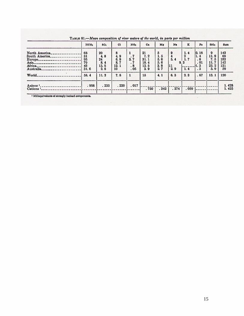
The elements are listed in Table 1-8 with their main species, range and meanseawater concentration (in molar units) and type of profile (from Chester, 2000). Table 1-9 shows the mean composition of the major components in rivers organized by continent.This is a logical format as different continents have different rock types.

Breakthroughs in analytical chemistry have been the leading edge for many of theperiods of rapid advances in understanding. Many examples were documented in thereviews by Spencer and Brewer (1970) and Johnson et al (1992). Some recent examplesinclude:- Graphite Furnace Atomic Absorption Spectrophotometry (GF-AAS) and Inductively

Coupled Plasma-Mass Spectrometry (ICP-MS) have led to rapid advances inunderstanding trace metal geochemistry. Multi-Detector ICP-MS has the potential todo so again in the near future by opening the new field of stable isotope geochemistryof trace metals.

- Improvements in polarographic techniques led to determination of the speciation oftrace metals (including iron) in seawater.

- Accelerator Mass Spectrometry (detecting atoms rather than radioactive decays) hasgreatly lowered the detection limit for 14C analyses thus reducing the requirements forsample size for radiocarbon analyses.

- Flow injection and microelectrode techniques have led to miniaturization andautomation of chemical analyses thus opening the door for more elaboratebiochemical moorings and drifters to obtain more extensive ocean time series. Withthe aid of satellite communication these can be established in remote locations whichmay be key for answering critical questions.

13

Modeling plays a big role in chemical oceanography. You need the followingtools. Box models, differential equations, sets of differential equations, and numericalmethods are routinely used tools for analysis of chemical oceanographic data. Thesetopics are introduced in Chapter 2. Students will find it useful to learn programs likeSTELLA, PHREEQ, MATLAB or MAPLE for transport reaction modeling andHYDRAQL, MINEQL+ or MINTEQA2 for chemical equilibrium modeling.

Chemical Oceanography is the most interdisciplinary of all the sub-disciplines of thisinterdisciplinary science.

- Chemical components of the ocean influence the density of seawater and thus effectits circulation.

- Oceanic-crustal coupling control the distribution of major ions (> 1 mg kg-1) inseawater on time scales of 104 to106 years. Thus, we can about weathering and othercrustal processes from ocean chemistry.

- Biological processes in the ocean are controlled by the chemistry. At the same timebiological processes are an important control on chemical distributions. The synergybetween biology and chemistry has led to a whole new thriving subdiscipline calledBiogeochemistry.

- Chemical components are tracers of physical, biological, geological and chemicalprocesses that make up the ocean that we observe. Understanding what controlschemical distributions helps us understand ocean dynamics.

- The Oceans are the ultimate reservoir of anthropogenic chemical perturbations.

- Chemical components of marine sediments and glacial ice provide clues necessary tounravel the history of past ocean chemistry and ocean-atmosphere dynamics.Understanding the past should help us predict the future.

14

15

16

Scope of Chemical Oceanography: Fundamental Questions

Here are a few examples of some of the key questions addressed in chemicaloceanography. Illustrated using classic examples from the literature. From this class youwill obtain the tools to address and understand these problems.

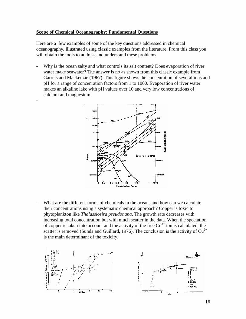
- Why is the ocean salty and what controls its salt content? Does evaporation of riverwater make seawater? The answer is no as shown from this classic example fromGarrels and Mackenzie (1967). This figure shows the concenration of several ions andpH for a range of concenration factors from 1 to 1000. Evaporation of river watermakes an alkaline lake with pH values over 10 and very low concentrations ofcalcium and magnesium.

-

- What are the different forms of chemicals in the oceans and how can we calculatetheir concentrations using a systematic chemical approach? Copper is toxic tophytoplankton like Thalassiosira pseudonana. The growth rate decreases withincreasing total concentration but with much scatter in the data. When the speciationof copper is taken into account and the activity of the free Cu2+ ion is calculated, thescatter is removed (Sunda and Guillard, 1976). The conclusion is the activity of Cu2+

is the main determinant of the toxicity.

17

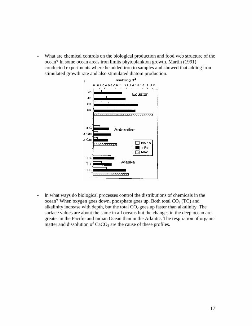
- What are chemical controls on the biological production and food web structure of theocean? In some ocean areas iron limits phytoplankton growth. Martin (1991)conducted experiments where he added iron to samples and showed that adding ironstimulated growth rate and also stimulated diatom production.

- In what ways do biological processes control the distributions of chemicals in theocean? When oxygen goes down, phosphate goes up. Both total CO2 (TC) andalkalinity increase with depth, but the total CO2 goes up faster than alkalinity. Thesurface values are about the same in all oceans but the changes in the deep ocean aregreater in the Pacific and Indian Ocean than in the Atlantic. The respiration of organicmatter and dissolution of CaCO3 are the cause of these profiles.

18

- What controls the distribution of clay minerals and biogenic phases like calcite(CaCO3(s)), opal (SiO2(s)) and organic carbon in marine sediments? CaCO3 isenriched in shallow sediments and almost totally absent in deep sediments. Whatcontrols this boundary? On the other hand, the distribution of SiO2 seems to reflectthe overlying biological production.

- What can chemical tracers (specific elements and compounds as well as stable andradioactive isotopes) tell us about physical, biological and geological processes andtheir rates in the ocean? For example, Craig et al (1973) used the distribution of 210Pbfrom the deep north Pacific to show that the residence time of Pb in the deep sea was54 years, rather than more like 5000 years as was commonly thought at the time.

19

- What is the role of the ocean in the global mass balance of C, N and O2? Keeling andShertz (1992) conducted simultaneous analyses of atmospheric CO2 and O2 andshowed that while both vary seasonally in opposite directions, there is also a longterm trend with CO2 increasing and O2 decreasing. This type of data gives us cluesabout the relative importance of marine versus terrestrial photosynthesis.

- How important is the ocean as a sink for fossil fuel CO2 and other greenhouse gases?Brewer (1978) calculated the pCO2 in samples from the core of the salinity minimumof the Antarctic Intermediate Water. The youngest samples from further south havehighest pCO2 reflecting the increase in atmospheric CO2.

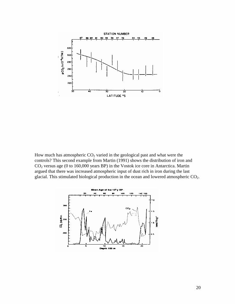
20

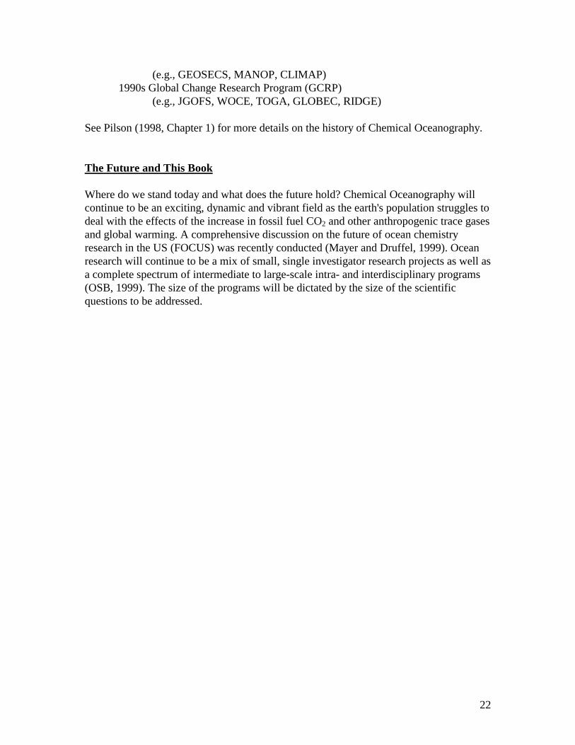
How much has atmospheric CO2 varied in the geological past and what were thecontrols? This second example from Martin (1991) shows the distribution of iron andCO2 versus age (0 to 160,000 years BP) in the Vostok ice core in Antarctica. Martinargued that there was increased atmospheric input of dust rich in iron during the lastglacial. This stimulated biological production in the ocean and lowered atmospheric CO2.

21

History

Chemical Oceanography has had a long and interesting history. Much of the earlydevelopment was tied to voyages of exploration (Schlee, 1973). The period since 1945has been one of immense progress in understanding the sea (Wunsch, 1993). Most of theadvances took place in the context of pure curiosity-driven basic science, as fundedinitially by the Office of Naval Research (ONR) and later by the National ScienceFoundation (NSF). Much of the funding for marine science was stimulated by itsperceived military implications driven by the Cold War between US and USSR. Sincethe fall of the Iron Curtain in 1989 there has been a period of declining support (inconstant dollars) .

Much of the early history was descriptive and chemical oceanography was consideredpart of biological oceanography until the 1960's. The stature of chemical oceanographygrew as it was realized that chemical tracers had the power to answer problems in alldisciplines of oceanography. By the 1970's the basic distribution of most elements hadbeen fairly well understood. At that time a subdiscipline of marine chemists emerged.These chemists focussed their efforts on understanding chemical reactions andmechanisms in the ocean and at its boundaries. Since the 1980's the field ofpaleoceanography has grown in importance as scientists attempt to extend ourunderstanding of the present day ocean into the geological past, especially the myriad ofperplexing problems associated with the glacial-interglacial cycles.

Some especially noteworthy events include:1772 Lavoisier produced the first respectable analyses of seawater and attempted to isolate some of its constituent salts.1836 Gay-Lussac showed that the total salt content of the ocean was remarkably

constant throughout the Atlantic. He suggested that the small differencesthat did exist were due to variations in river runoff as well as evaporationand precipitation

1819 Marcet analyzed seawater from several different locations and determinedthat there was a constant proportion between the major elements. We nowrefer to this fundamental concept as Marcet's Principle or The Principle ofConstant Proportions.

1865 Forchhammer presented the first definition of salinity1884 Dittmar completed the first systematic analyses of the major ions in

seawater. He used samples collected during the HMS ChallengerExpedition (1873-1876)

1930s Rockefeller Foundation provided support to strengthen oceanographicprograms at Scripps Institution of Oceanography, the Woods HoleOceanographic Institution and the University of Washington.

1940s World War II, which led to the building of the ocean research establishment. Congress created the Office of Naval Research (ONR) in 1946.1970s International Decade of Ocean Exploration (IDOE)

22

(e.g., GEOSECS, MANOP, CLIMAP)1990s Global Change Research Program (GCRP)

(e.g., JGOFS, WOCE, TOGA, GLOBEC, RIDGE)

See Pilson (1998, Chapter 1) for more details on the history of Chemical Oceanography.

The Future and This Book

Where do we stand today and what does the future hold? Chemical Oceanography willcontinue to be an exciting, dynamic and vibrant field as the earth's population struggles todeal with the effects of the increase in fossil fuel CO2 and other anthropogenic trace gasesand global warming. A comprehensive discussion on the future of ocean chemistryresearch in the US (FOCUS) was recently conducted (Mayer and Druffel, 1999). Oceanresearch will continue to be a mix of small, single investigator research projects as well asa complete spectrum of intermediate to large-scale intra- and interdisciplinary programs(OSB, 1999). The size of the programs will be dictated by the size of the scientificquestions to be addressed.

23

Don't be shy. Ask Questions!

24

Relevant Web Sites:

1. Saewifs images including the Ocean and Terrestrial Biosphere//seawifs.gsfc.nasa.gov/SEAWIFS/IMAGES/

2. Several 3-D images, the age of the ocean crust and total sediment thicknessftp//ftp.ngdc.noaa.gov/mgg/images

3. TOGA/TAO array data from the equatorial Pacific//www.pmel.noaa.gov/toga-tao/realtime.html

4. Online Map Creation//www.aquarius.geomar.de/omc

References:

Berner E.K. and R.A. Berner (1987) The Global Water Cycle. Prentice-Hall, Inc.,Englewood Cliffs, NJ, 397pp.

Brewer P.G. (1978) Direct observation of the Oceanic CO2 increase. Geophys. Res. Lett.,5, 997-1000.

Butcher S.S., R.J. Chrlson, G.H. Orians and G.V. Wolfe (eds)(1992) GlobalBiogeochemical Cycles. Academic Press, San Diego, 379 pp.

Craig H., S. Krishnaswami and B.L.K. Somayajulu (1973) 210Pb-226Ra: Radioactivedisequilibria in the deep sea. Earth and Planet Science Letters, 17, 295-305.

Forchhammer G. (1865) On the composition of seawater in different parts of the ocean.Philos. Trans. R. Soc. London. 155, 203-262.

Garrels R.M. and F.T. Mackenzie (1967) Origin of the chemical compositions of somesprings and lakes. In (W. Stumm, ed) Equilibrium Concepts in Natural Water Systems.Advances in Chemistry Series 67, ACS, Washington, 222- 242.

Johnson K.S., K.H. Coale and H.W. Jannasch (1992) Analytical Chemistry inOceanography. Analytical Chemistry, 64, 1065A-1075A

Keeling C.D. et al (1976) Atmospheric carbon dioxide variations at Mauna LoaObservatory, Hawaii. Tellus, 28, 538-551.

Keeling R.F. and S.R. Shertz (1992) Seasonal and interannual variations in atmosphericoxygen and implications for the global carbon cycle. Nature, 358, 723-727.

Libes S. (1992) Marine Biogeochemistry. Wiley, New York, 734pp.

25

Livingston D.A. (1963) Chapter G. Chemical Composition of Rivers and Lakes. In (M.Fleischer, ed) Data of Geochemistry, Sixth Edition. USGS Prof. Pap. 440-G, 64 pp.

Martin J.H. (1991) Iron, Liebig's Law and the Greenhouse. Oceanography, 4, 52-55.

Mayer L. And E. Druffel (eds)(1999) The Future of Ocean Chemistry in the US., UCAR,151pp.

Millero F. J. (1996) Chemical Oceanography, 2nd Edition. CRC Press, Boca Raton,469pp.

Morel F.M.M. and J.G. Hering (1993) Principles and Applications of Aquatic Chemistry.Wiley, New York, 588pp.

Ocean Studies Board (1999) Global Ocean Science: Toward an Integrated Approach.National Academy Press, Washington, 165pp.

Parker R.L. (1967) Chapter D. Composition of the Earth's Crust. In (M. Fleischer, ed)Data of Geochemistry, Sixth Edition. USGS Prof. Paper 440-D. 19pp.

Pilson M.E.Q. (1998) An Introduction to the Chemistry of the Sea. Prentice Hall, NewJersey, 431pp.

Reeburgh W.S. (1997) Figures summarizing the Global Cycles of BiogeochemicallyImportant Elements. Bull. Ecol. Soc. Amer., 78, 260-267.

Schlee S. (1973) The Edge of an Unfamiliar World: A History of Oceanography. P.Dutton & Co., New York.

Schwarzenbach R.P , P.M. Gschwend and D.M. Imboden (1993) Environmental OrganicChemistry. Wiley, New York, 681pp.

Spencer D.W. and P.G. Brewer (1970) Analytical Methods in Oceanography I. Inorganicmethods. CRC Critical Reviews in Solid State Sciences, 409-478.

Stumm W. and J.J. Morgan (1996) Aquatic Chemistry, 3rd Edition. Wiley, New York,1022pp.

Sunda W. and R.R.L. Guillard (1976) The relationship between cupric ion activity andthe toxicity of copper to phytoplankton. J. Mar. Res., 34, 511-529.

USGCRP (1999) A U.S. Carbon Cycle Science Plan.

Wunsch C. (1993) Marine Sciences in the Coming Decades. Science, 259, 296-297.