with (C) Pearson Education Adapted by Michael Hahsler

Data mining is focused on better understanding of characteristics and patterns among variables in large databases using a variety of statistical and analytical tools.

It is used to identify relationships among variables in large data sets and understand hidden patterns that they may contain

Clustering Identify groups with elements that are in some way similar to each

other.

Classification Analyze data to predict how to classify a new data element.

Association Analysis Analyze databases to identify natural associations among

variables and create rules for target marketing or buying recommendations.

Real data sets that have missing values or errors. Such data sets are called “dirty” and need to be “cleaned” prior to analyzing them.

Approaches for handling missing data. ◦ Eliminate the records that contain missing data ◦ Estimate reasonable values for missing observations, such as the mean

or median value

Try to understand whether missing data are simply random events or if there is a logical reason. Eliminating sample data indiscriminately could result in misleading information and conclusions about the data.

Rapidminer: • Blending (e.g., sampling) • Cleansing

Cluster analysis (data segmentation) tries to group or segment a collection of objects into clusters, such that those within each cluster are more closely related to one another than to objects assigned to different clusters. The true grouping is typically not known (=unsupervised learning).

Descriptive Analytics

How do we measure similarity? Example: Euclidean distance is the straight-line

distance between two points. The Euclidean distance measure between two

points x = (x1, x2, . . . , xn) and y = (y1, y2, . . . , yn) is

Data should be normalized (scaled) before calculating distances. Rapidminer: Cleansing - Normalization

d(x, y) =

There exist many other distance measures! E.g., for categorical and mixed data.

12-7

• 50 samples from each of three species of Iris (Iris setosa, Iris virginica and Iris versicolor).

• 4 features were measured from each sample: the length and the width of the sepals and petals (in cm)

Examples: Sepal length

Sepal width

Petal length

Petal width Species

5.1 3.5 1.4 0.2 I. setosa 4.9 3 1.4 0.2 I. setosa 4.7 3.2 1.3 0.2 I. setosa 4.6 3.1 1.5 0.2 I. setosa

12-8

k-means clustering aims to partition n observations into k clusters in which each observation belongs to the cluster with the nearest mean, serving as a prototype of the cluster.

z-score

Only choose a1, a2, a3, a4 for clustering

Choose k and distance measure

(Euclidean)

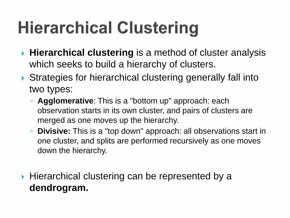
Hierarchical clustering is a method of cluster analysis which seeks to build a hierarchy of clusters.

Strategies for hierarchical clustering generally fall into two types: ◦ Agglomerative: This is a "bottom up" approach: each

observation starts in its own cluster, and pairs of clusters are merged as one moves up the hierarchy.

◦ Divisive: This is a "top down" approach: all observations start in one cluster, and splits are performed recursively as one moves down the hierarchy.

Hierarchical clustering can be represented by a

dendrogram.

Divisive Methods

Agglomerative Methods

Dendrogram

Dis

tanc

e

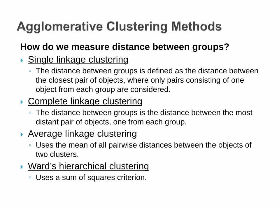
How do we measure distance between groups? Single linkage clustering ◦ The distance between groups is defined as the distance between

the closest pair of objects, where only pairs consisting of one object from each group are considered.

Complete linkage clustering ◦ The distance between groups is the distance between the most

distant pair of objects, one from each group. Average linkage clustering ◦ Uses the mean of all pairwise distances between the objects of

two clusters. Ward’s hierarchical clustering ◦ Uses a sum of squares criterion.

Dendrogram

Use Flattern Clustering to get cluster assignments (i.e.,

cut the dendrogram at a given number of clusters)

Select and normalize attributes

Analyze each cluster separately (e.g., group-wise means, bar charts)

Give each cluster a label depending on the objects in the cluster (e.g., large flowers for the iris data set)

Use the cluster group as an input for other models (e.g., regression or classification)

Classification is the problem of predicting to which of a set of categories a new observation belongs, on the basis of a training set of data containing observations whose category membership is known (=supervised learning).

Similar to regression, but the outcome is categorical (often yes/no).

Predictive Analytics

Define class variable as role “label”

Find the probability of making a misclassification error.

Represent the results in a confusion matrix, which shows the number of cases that were classified either correctly or incorrectly.

Summarize the error rate into a single value. For example accuracy or kappa. Both measure the chance of making a correct prediction.

12-17

Confusion Matrix with Accuracy

Predicted labels (and confidence of prediction)

Testing on the data used for training is not a good idea. We are more interested in how the model performs on new data!

The data can be partitioned into: ▪ training data set – has known outcomes and is

used to “teach” the data-mining algorithm ▪ test data set – tests the accuracy of the model

80% training / 20% testing is very common.

12-19 You will get a confusion matrix for the test data.

k-Nearest Neighbors (k-NN) Algorithm Finds records in a database that have similar

numerical values of a set of predictor variables

Logistic Regression Estimates the probability of belonging to a category

using a regression on the predictor variables.

Measure the Euclidean distance between records in the training data set.

The nearest neighbor to a record in the training data set is the one that that has the smallest distance from it. ◦ If k = 1, then the 1-NN rule classifies a record in the same category as its

nearest neighbor. ◦ k-NN rule finds the k-Nearest Neighbors in the training data set to each

record we want to classify and then assigns the classification as the classification of majority of the k nearest neighbors

Typically, various values of k are used and then results inspected to determine which is best.

Logistic regression is variation of linear regression in which the dependent variable is binary (0/1 or True/False).

Predicts probabilities. Usually if the predicted

probability for 1 is >50% then class 1 is predicted.

Estimate the probability p that an observation belongs to category 1, P(Y = 1), and, consequently, the probability 1 - p that it belongs to category 0, P(Y = 0).

Then use a cutoff value, typically 0.5, with which to compare p and classify the observation into one of the two categories.

The dependent variable is called the logit, which is the natural logarithm of p/(1 – p) – called the odds of belonging to category 1.

The form of a logistic regression model is

The logit function can be solved for p:

Just replace the classification operator in Rapid Miner with whatever model you like.

12-24

Association rule mining, often called affinity analysis, seeks to uncover associations and/or correlation relationships in large binary data sets

◦ Association rules identify attributes that occur together

frequently in a given data set. ◦ Market basket analysis, for example, is used determine

groups of items consumers tend to purchase together.

Association rules provide information in the form of if-then (antecedent-consequent) statements.

Descriptive Analytics

PC Purchase Data We might want to know which components are often

ordered together.

trans

actio

ns

items

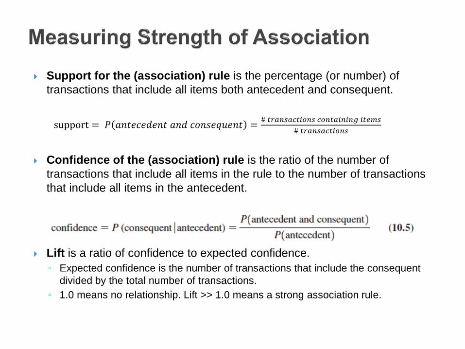
Support for the (association) rule is the percentage (or number) of transactions that include all items both antecedent and consequent.

support = 𝑃 𝑎𝑎𝑎𝑎𝑎𝑎𝑎𝑎𝑎𝑎 𝑎𝑎𝑎 𝑎𝑐𝑎𝑐𝑎𝑐𝑐𝑎𝑎𝑎 = # 𝑡𝑡𝑡𝑡𝑡𝑡𝑡𝑡𝑡𝑡𝑡𝑡 𝑡𝑡𝑡𝑡𝑡𝑡𝑡𝑡𝑡𝑐 𝑡𝑡𝑖𝑖𝑡

# 𝑡𝑡𝑡𝑡𝑡𝑡𝑡𝑡𝑡𝑡𝑡𝑡

Confidence of the (association) rule is the ratio of the number of

transactions that include all items in the rule to the number of transactions that include all items in the antecedent.

Lift is a ratio of confidence to expected confidence. ◦ Expected confidence is the number of transactions that include the consequent

divided by the total number of transactions. ◦ 1.0 means no relationship. Lift >> 1.0 means a strong association rule.

A supermarket database has 100,000 point-of-sale transactions; 2000 include both A and B items; 5000 include C; and 800 include A, B, and C

Association rule: {A , B} => C (“If A and B are purchased, then C is also purchased.”) Support = 800/100,000 = 0.008 Confidence = 800/2000 = 0.40 Expected confidence = 5000/100,000 = 0.05 Lift = 0.40/0.05 = 8

12-29

Data mining offers many methods for descriptive and predictive analytics.

Different methods work better for different data sets.

It is often not clear which method to use and most analytics professionals will try and compare several methods.

The most critical part is cleaning and preparing the data and to ask the right questions.

30