Embed Size (px)
Citation preview

(Lesson 1: Intro; Ch.1) 1.01
CHAPTER 1: INTRODUCTION
LESSON 1: INTRODUCTION
PART A: STRUCTURE OF THE TEXT
(4TH
EDITION OF TRIOLA’S ESSENTIALS)
Statistics Probability (Chapters 4-6)
|
1) Designing an Experiment |
(Chapter 1) |
|
2) Collecting Data |
(Chapter 1) |
|
3) Describing Data |
(Chapters 2, 3) |
|
4) Interpreting Data using
(Chapters 3, 7-11)
Size: N elements (or members)
Population [of interest] All adult Americans?
All registered voters in California?
2) 4)
Size: n elements (or members)
Sample For a poll? A scientific study?
The Nielsens?
3)
The population must be carefully defined. For example …
• Do “adult Americans” include illegal immigrants?
• Different polls of “likely U.S. voters” use different models for the
purposes of screening poll respondents. Voter enthusiasm and
voting history may be issues.

(Lesson 1: Intro; Ch.1) 1.02
PART B: COLLECTING DATA; SAMPLING METHODS
If we manage to collect data from each element of the population, we have
ourselves a census. Often, a census is impossible or impractical, so we collect data
on only some elements of the population. These elements make up a sample from
the population.
How do we select a sample so that it is representative of the overall population?
Section 1-4 details a number of methods. We will discuss related issues later, when
we discuss polls in Chapter 7.
A common problem in practice is the use of overly homogeneous samples in
which the elements within the sample are much more similar than is the case
within the overall population. For example, you wouldn’t want to restrict
your sample to a single state if you wanted to study the national popularity
of the President.
We will typically assume that a sample from a population is a simple random
sample (SRS). When constructing an SRS, each group of n elements in the
population is equally likely to be our selected sample of n elements.
Example
If n = 4 , then the two samples below (each represented by four black
squares) are equally likely to be selected:
Note: When constructing a random sample in general, each individual
element is equally likely to be among those selected for the sample, but
some groups of n elements may be more likely to be selected than others.
Selections could be linked.

(Lesson 1: Intro; Ch.1) 1.03
In systematic sampling, the elements of the population are ordered, and, after some
point, every kth
element is selected (where k is some integer greater than 1).
Example
We can select every third person that enters a particular bookstore on
a particular day. Here, k = 3.
Skip Skip Select Skip Skip Select Skip Skip Select

(Lesson 2: Frequency Tables; 2-2) 2.01
CHAPTERS 2: DESCRIPTIVE STATISTICS I
How can we efficiently and effectively summarize data or compare data from two or
more populations?
LESSON 2: FREQUENCY TABLES (SECTION 2-2)
Example
Let’s summarize the ages (in years) at which the 43 U.S. Presidents became
President (as of 2007). The complete list of 43 ages may not be so appealing to
people!
The ages will be grouped into classes. Triola suggests using between 5 and 20
classes.
The frequency of each age class is the number of Presidential ages that lie within
that class.
The relative frequency of each age class is obtained by dividing the corresponding
frequency by N, which is the population size. Here, N = 43. The decision to round
off relative frequencies to three decimal places was an arbitrary one.
Age
classes
Frequency Relative
Frequency
Relative
Frequency
(as a percent)
35-39 0 0 0%
40-44 2 0.047 4.7%
45-49 6 0.140 14.0%
50-54 13 0.302 30.2%
55-59 12 0.279 27.9%
60-64 7 0.163 16.3%
65-69 3 0.070 7.0%
70+ 0 0 0%
Sum = N
= 43 Sum = 1 Sum = 100%

(Lesson 2: Frequency Tables; 2-2) 2.02
Note on Rounding: Triola obsesses over this issue, but the rounding issue really
depends on the application. Here, we have rounded down ages.
Note on Roundoff Error: The rounded off values in the “Relative Frequency”
column actually add up to 1.001, but we shouldn’t worry about this. If the sum
were something like 2, then we should worry!
Note on Trailing Zeros: Why, for instance, do we write “0.140” as opposed to
simply “0.14”? The trailing zero at the end of “0.140” indicates that 0.140 is
accurate to three decimal places. Given that we are rounding off relative
frequencies to three decimal places, the “0.14” might be mistaken to be an exact
value.
Note on Classes: Observe that the classes are the same size, with the exception of
the “70+” class. We typically avoid using classes of unequal size: for example,
40-49 and 50-54. Also, the “35-39” class was included because 35 is the minimum
required age for the U.S. Presidency mandated by the Constitution.
Historical Notes: We are counting Grover Cleveland twice, because he served two
nonconsecutive terms. The youngest President was Teddy Roosevelt, who was 42
when he succeeded William McKinley on his assassination. John Kennedy was the
youngest elected President at the age of 43. Ronald Reagan was the oldest elected
President at the age of 69.
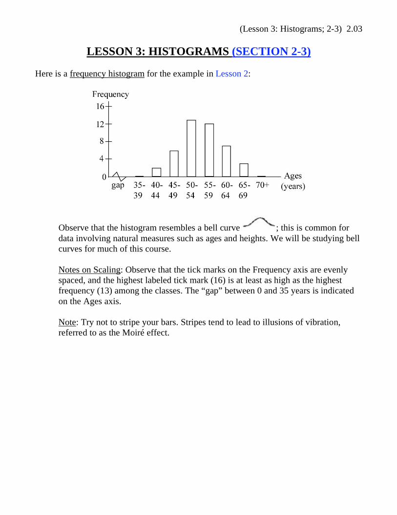
(Lesson 3: Histograms; 2-3) 2.03
LESSON 3: HISTOGRAMS (SECTION 2-3)
Here is a frequency histogram for the example in Lesson 2:
Observe that the histogram resembles a bell curve ; this is common for
data involving natural measures such as ages and heights. We will be studying bell
curves for much of this course.
Notes on Scaling: Observe that the tick marks on the Frequency axis are evenly
spaced, and the highest labeled tick mark (16) is at least as high as the highest
frequency (13) among the classes. The “gap” between 0 and 35 years is indicated
on the Ages axis.
Note: Try not to stripe your bars. Stripes tend to lead to illusions of vibration,
referred to as the Moiré effect.
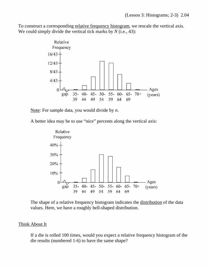
(Lesson 3: Histograms; 2-3) 2.04
To construct a corresponding relative frequency histogram, we rescale the vertical axis.
We could simply divide the vertical tick marks by N (i.e., 43):
Note: For sample data, you would divide by n.
A better idea may be to use “nice” percents along the vertical axis:
The shape of a relative frequency histogram indicates the distribution of the data
values. Here, we have a roughly bell-shaped distribution.
Think About It
If a die is rolled 100 times, would you expect a relative frequency histogram of the
die results (numbered 1-6) to have the same shape?

(Lesson 4: More Statistical Graphics; 2-4) 2.05
LESSON 4: MORE STATISTICAL GRAPHICS (SECTION 2-4)
Look at my MINITAB handout.
PART A: DOTPLOTS
These are like histograms with many “thin” classes, except that stacked dots
replace the bars.
PART B: STEMPLOTS, OR STEM-AND-LEAF PLOTS
These resemble sideways histograms, but you can use them to:
• recover the original data values
• sort the data values (i.e., place them in numerical order)
Example
Nine students take a test. Their scores are as follows:
77 93 73 51 74 85 82 73 100
Stage 1: Assign leaves to stems.
The leaf of a data value is the value’s last digit.
The stem consists of the other digits.
Note: If the data values are not integers, they must be written
out to the same number of decimal places.
Write the stems in increasing order.
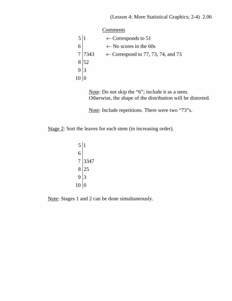
(Lesson 4: More Statistical Graphics; 2-4) 2.06
Comments
5
6
7
8
9
10
1 Corresponds to 51
No scores in the 60s
7343 Correspond to 77, 73, 74, and 73
52
3
0
Note: Do not skip the “6”; include it as a stem.
Otherwise, the shape of the distribution will be distorted.
Note: Include repetitions. There were two “73”s.
Stage 2: Sort the leaves for each stem (in increasing order).
5
6
7
8
9
10
1
3347
25
3
0
Note: Stages 1 and 2 can be done simultaneously.

(Lesson 4: More Statistical Graphics; 2-4) 2.07
PART C: SCATTERPLOTS, OR SCATTER DIAGRAMS
We will discuss these further in Chapter 10.
These are for paired data of the form
xi, y
i( ) .
Example
In the MINITAB handout, student # i received a score of x
i on
Midterm 1 and a score of y
i on Midterm 2. 1 i N = 92( )
Beware of abuse! Rescaling axes can dramatically change the picture.
PART D: TIME-SERIES GRAPHS
Example
Year U.S. Population
(in millions)
1920 106
1940 132
1960 179
1980 227
2000 281

(Lesson 4: More Statistical Graphics; 2-4) 2.08
Thus far, we have been dealing with quantitative data, the most common form of
numerical data.
We will now look at qualitative data.
PART E: PARETO CHARTS
Example
Political parties of the 43 U.S. Presidents (as of 2007):
Party affiliation Frequency
Democrats (D) 15
Republicans (R) 18
Whigs (W) 4
Other 6
Historical Note: The six “Others” included four Democratic-
Republicans and two Federalists.
A Pareto chart resembles a histogram, except that the horizontal axis is
organized by categories, not by quantitative measurements. The categories
are listed in descending order of frequency.

(Lesson 4: More Statistical Graphics; 2-4) 2.09
PART F: PIE CHARTS
Example (Presidential Parties again)
Again, we have:
Party affiliation Frequency
Democrats (D) 15
Republicans (R) 18
Whigs (W) 4
Other 6
N = 43.
For each party, the relative frequency is given by:
Frequency
43.
The measure of the central angle of the corresponding pie slice is given by:
Relative Frequency( ) 360( ) . Remember that there are 360 degrees in a
full counterclockwise revolution sweeping out the boundary circle.
Here, we will round off relative frequencies to three decimal places and
angle measures to the nearest degree.
Party affiliation Frequency Relative
Frequency
Measure of
Central
Angle
Democrats (D) 15 0.349 (34.9%) 126
Republicans (R) 18 0.419 (41.9%) 151
Whigs (W) 4 0.093 (9.3%) 33
Other 6 0.140 (14.0%) 50

(Lesson 5: Measures of Center; 3-2) 3.01
CHAPTERS 3: DESCRIPTIVE STATISTICS II
LESSON 5: MEASURES OF CENTER (SECTION 3-2)
PART A: FOUR MEASURES
Example 1
The five students in a class take a test. Their scores in points are as follows:
80 76 100 83 100
How can we find a single number that tells us how well the class did?
Let’s look at four possibilities for measuring the center of a data set.
1) [Arithmetic] Mean or Average
There are other measures called means, but the arithmetic mean (or simply
“the mean”) is by far the most common.
In Our Example
Mean =Sum of all data values
Number of values
=80 + 76 +100 + 83+100
5
=439
5
= 87.8 points
Warning: You must group or compute (“process”) the numerator
before dividing by 5. You can do this by either placing grouping
symbols like parentheses around the numerator, or by pressing
“ENTER” or the like on your calculator before dividing. What would
be wrong with entering the following on your calculator:
80 + 76 +100 + 83+100 ÷ 5 = ?
Remember to write units, such as “points”, in your final answer where
appropriate.
(Lesson 5: Measures of Center; 3-2) 3.02
Notes on Rounding:
• In Chapter 3, we will typically round off our final answers to
one more decimal place than the number of decimal places
provided in the given data. In this Example, because the given
data values are integers (rounded off to zero decimal places),
we round off our final answers to one decimal place.
• Avoid rounding intermediate results, however. This becomes
an issue in later sections. Triola suggests rounding off
intermediate results to at least twice as many decimal places as
will be present in your final answer, but this might not be
enough.
• Always read instructions on exams. They take precedence
over everything.
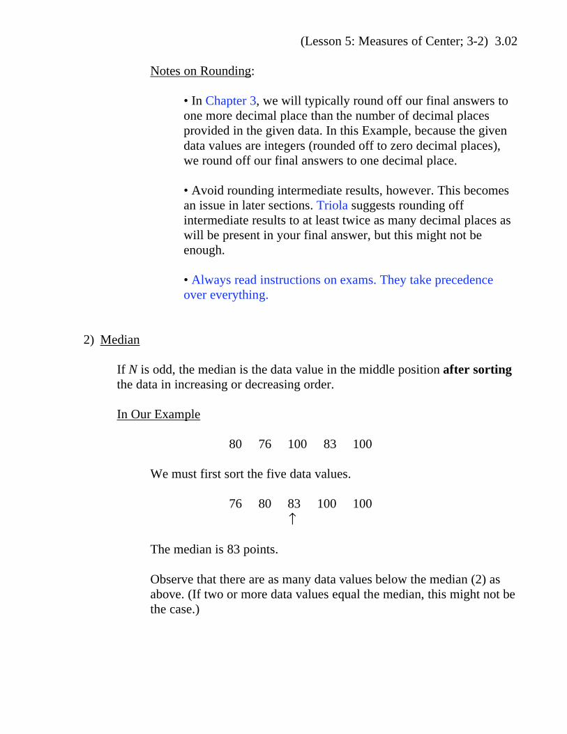
2) Median
If N is odd, the median is the data value in the middle position after sorting
the data in increasing or decreasing order.
In Our Example
80 76 100 83 100
We must first sort the five data values.
76 80 83 100 100
The median is 83 points.
Observe that there are as many data values below the median (2) as
above. (If two or more data values equal the median, this might not be
the case.)

(Lesson 5: Measures of Center; 3-2) 3.03
If N is even, the median is the average of (i.e., the midpoint between) the
two data values in the two middle positions after sorting the data.
Modified Example
Let’s say there were only four test scores:
80 76 100 83
We must first sort them.
76 80 83 100
The two middle values are 80 and 83, so we take their average,
80 + 83
2= 81.5 . The median is 81.5 points.
3) Mode
The mode is the most frequent data value, if any, in the data set.
A data set could have no mode, one mode, or more than one mode.
It is sometimes denoted by x̂ .
In Our Example
80 76 100 83 100
The mode is 100 points. (How wonderful!)
(We do not have to go one decimal point further for modes.)
Although it is often easy to find modes, they might be questionable as
measures of centrality. The mode may actually be an extreme value, as in
our Example, or it may just be the consequence of simple coincidence.
Example: The data set
2.41, 3.62, 7.25{ } has no mode.
Example: The data set
50, 50, 70, 90, 90{ } has two modes, 50 points and 90
points. The data set is bimodal.
(Lesson 5: Measures of Center; 3-2) 3.04
The mode can also be used for qualitative data, such as the political party
data set in Lesson 4.
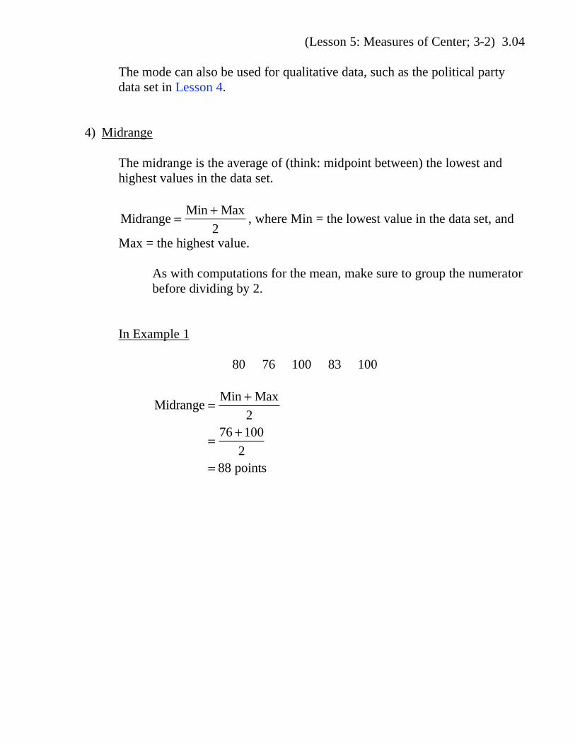
4) Midrange
The midrange is the average of (think: midpoint between) the lowest and
highest values in the data set.
Midrange =Min + Max
2, where Min = the lowest value in the data set, and
Max = the highest value.
As with computations for the mean, make sure to group the numerator
before dividing by 2.
In Example 1
80 76 100 83 100
Midrange =Min + Max
2
=76 +100
2
= 88 points

(Lesson 5: Measures of Center; 3-2) 3.05
PART B: NOTATION
We can label data values xi, where 1 i N for population data, or 1 i n for
sample data.
In Example 1
We have a population data set of size N = 5 .
x
1
x
2
x
3
x
4
x
5
80 76 100 83 100
Summation Notation
The Greek uppercase sigma,
, is a summation operator.
x denotes the sum of the given data values.
More precisely:
xi
i=1
N
= x1+ x
2+…+ x
N denotes the sum of the values in a population
data set, and
xi
i=1
n
= x1+ x
2+…+ x
n denotes the sum in a sample data set.
In Example 1:
xi
i=1
5
= x1+ x
2+ x
3+ x
4+ x
5.
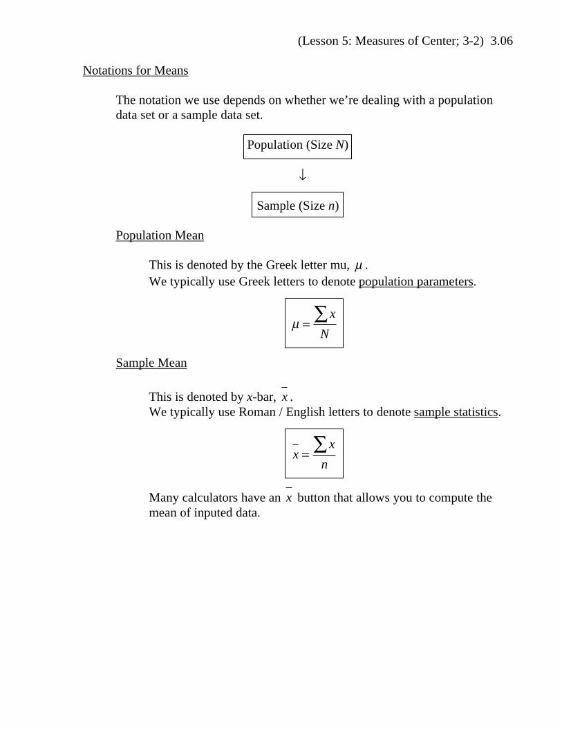
(Lesson 5: Measures of Center; 3-2) 3.06
Notations for Means
The notation we use depends on whether we’re dealing with a population
data set or a sample data set.
Population (Size N)
Sample (Size n)
Population Mean
This is denoted by the Greek letter mu, μ .
We typically use Greek letters to denote population parameters.
μ =x
N
Sample Mean
This is denoted by x-bar, x .
We typically use Roman / English letters to denote sample statistics.
x =x
n
Many calculators have an x button that allows you to compute the
mean of inputed data.

(Lesson 5: Measures of Center; 3-2) 3.07
PART C: MEAN VS. MEDIAN; OUTLIERS
Example 2
The five students in a class take a test. Their test scores in points are as
follows:
100 90 90 80 70
Median = 90 points
Mean = 86 points
Let’s say the person who received the “70” actually cheated, and we drop
that score down to 0 points. What effect does that have on the median and
the mean?
100 90 90 80 0
Median = 90 points
Mean = 72 points
Outliers
The “0” is an outlier, because it is extremely high or low relative to the other
data values.
The mean is sensitive to outliers, and it exhibits a dramatic drop.
The median is not sensitive to outliers, and it remains unchanged in our
Example.
The midrange is very sensitive to outliers; it drops from 85 points down to
50 points in our Example.
(Lesson 5: Measures of Center; 3-2) 3.08
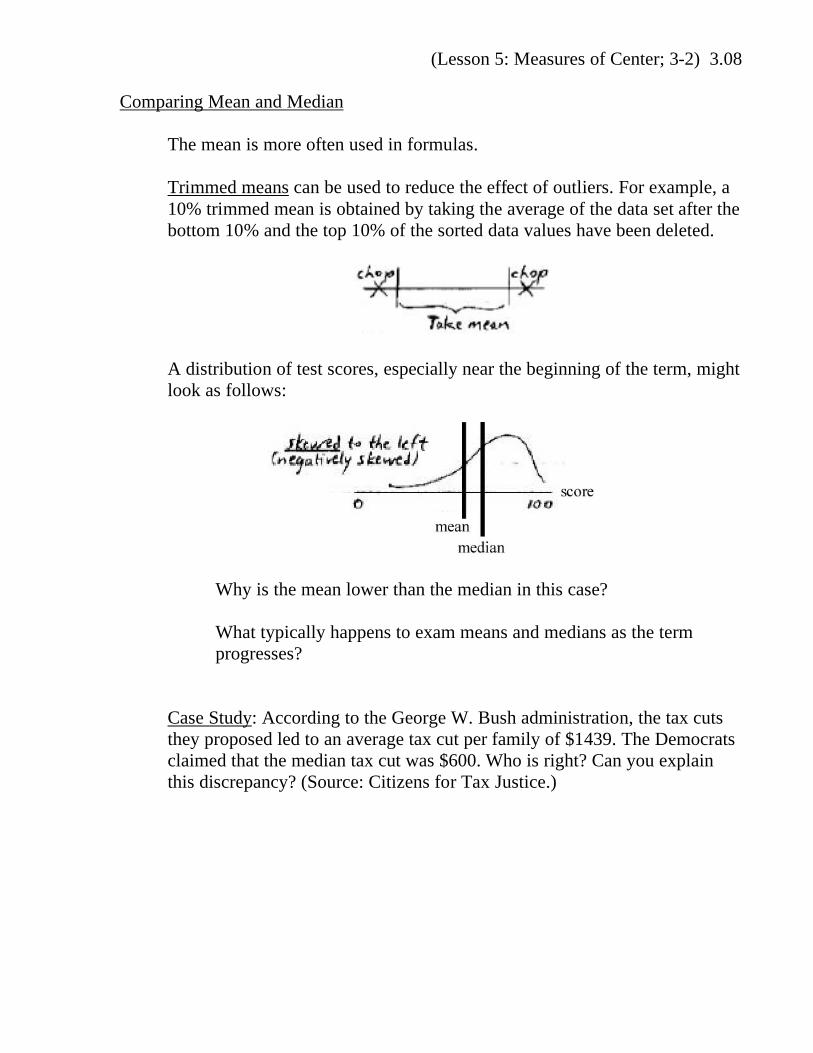
Comparing Mean and Median
The mean is more often used in formulas.
Trimmed means can be used to reduce the effect of outliers. For example, a
10% trimmed mean is obtained by taking the average of the data set after the
bottom 10% and the top 10% of the sorted data values have been deleted.
A distribution of test scores, especially near the beginning of the term, might
look as follows:
Why is the mean lower than the median in this case?
What typically happens to exam means and medians as the term
progresses?
Case Study: According to the George W. Bush administration, the tax cuts
they proposed led to an average tax cut per family of $1439. The Democrats
claimed that the median tax cut was $600. Who is right? Can you explain
this discrepancy? (Source: Citizens for Tax Justice.)

(Lesson 5: Measures of Center; 3-2) 3.09
PART D: ESTIMATING THE MEAN FROM A FREQUENCY TABLE
Example 3
Following state requirements, 28 math teachers take a statistics test. Their
test scores in points are described by the following frequency table:
Score Classes Frequency
f( )
50-59 2
60-69 4
70-79 7
80-89 10
90-99 5
Estimate the mean of the test scores.
Solution to Example 3
We are faced with limited, “grainy” information about the data set.
We will replace each score class with its class mark, the midpoint of the
class. For example, the class mark for the “60-69” class will be:
60 + 69
2= 64.5 points . We are “boiling down” the classes into their marks.
Note: If the data values had been rounded down, as is the case with ages,
then 65 points may be a more appropriate choice for the class mark.
As a simplifying assumption, we are assuming that all four students in the
class received a score of 64.5 points on the test. More generally, we could
also assume that the average of the four students’ scores is 64.5 points.
(Either assumption will have the same impact on our estimate of the mean.)
Either way, our estimate for the sum of the four students’ scores will be:
64.5+ 64.5+ 64.5+ 64.5 = 4( ) 64.5( ) = 258 points . In general, our estimated
“class sum” (i.e., the sum of the scores within a class) is given by f x ,
where f is the class frequency and x is the class mark. We will then add
these class sums to obtain our estimate for the sum of all of the scores,
f x .

(Lesson 5: Measures of Center; 3-2) 3.10
This scheme does not automatically bias our estimate towards either the low
end or the high end.
Score Classes Frequency
f( )
Class Marks
x( )
50-59 2 54.5
60-69 4 64.5
70-79 7 74.5
80-89 10 84.5
90-99 5 94.5
N = f
= 28
Estimated Mean =Estimated Sum
N
=f x
N
=2( ) 54.5( ) + 4( ) 64.5( ) + 7( ) 74.5( ) + 10( ) 84.5( ) + 5( ) 94.5( )
28
=2206
28We've processed the numerator before dividing.( )
78.8 points (indicates end of solution)
Think About It: If we had used 55, 65, etc. as our class marks, how would
our estimate have changed?
Think About It: Why is our estimated mean closer to the 90s than to the 50s?
A related issue is coming up ….

(Lesson 5: Measures of Center; 3-2) 3.11
PART E: WEIGHTED MEANS
In some data sets, some values are more important than others. We use weights to
measure the relative importance of data values.
Think About It: If you get an “A” on a midterm worth 10% of a class and an “F”
on a final worth 90% of the class, does that mean you will pass with a “C”?
Example 4 (GPA)
If you receive the following grade report for a term, what is your grade point
average (GPA) for the term?
Course
Number
of Units
(Weights, w)
Grade
Math 5 A-
Chemistry 4 D
Biology 3 C+
GPA Scheme
The grades are ordinal data values. They are nonnumeric, but there is
a natural order among the possible grades: A+, A, A-, B+, etc.
We will recode the grades as quantitative numeric data as follows:
A = 4
B = 3
C = 2
D = 1
F = 0
The “+” modifier raises the value by 0.3.
The “-” modifier lowers the value by 0.3.
The “A-“ grade in Math, for example, corresponds to: 4 0.3= 3.7 .

(Lesson 5: Measures of Center; 3-2) 3.12
Because the Math class is worth five units, imagine writing 3.7 on five
slips of paper. Similarly, imagine writing 1.0 (corresponding to the
“D”) on four slips and 2.3 (corresponding to the “C+”) on three slips.
Our weighted mean or average will then simply be the arithmetic
mean of the numbers on all 12 slips.
Sums: w x , where:
w = number of units, and
x = grade value
3.7 3.7 3.7 3.7 3.7 5( ) 3.7( )
1.0 1.0 1.0 1.0 4( ) 1.0( )
2.3 2.3 2.3 3( ) 2.3( )
Grand sum = w x
Solution to Example 4
GPA =Grand sum
Sum of all weights i.e., total number of units( )
=w x
w
=5( ) 3.7( ) + 4( ) 1.0( ) + 3( ) 2.3( )
5+ 4 + 3
=29.4
12
= 2.45 grade points
Would this be good enough for medical school in the U.S.?

(Lesson 5: Measures of Center; 3-2) 3.13
Example 5 (Course grade)
You receive the following scores in a class:
Exam
% of
Course
Grade
Score
(out of
100 points)
Quiz 1 10% 75
Quiz 2 10% 80
Quiz 3 10% 100
Midterm 25% 95
Final 45% a
You have not yet taken the Final, so we have labeled the Final score with a
hopeful “a”.
What must you get on the Final to get at least 90% in the course overall
(that is, at least 90 points as a weighted average)?
Solution to Example 5
Again, we are asking about a weighted mean. Observe that the Final is worth
much more than any other exam.
We will write the exam weights as decimals: 0.10 for 10%, etc.
Course average =w x
w
=0.10( ) 75( ) + 0.10( ) 80( ) + 0.10( ) 100( ) + 0.25( ) 95( ) + 0.45( ) a( )
1
= 49.25+ 0.45a
Warning: Do not combine the unlike terms 49.25 and 0.45a as 49.70a; that
is wrong!
We have expressed your course average as a function of a, the score on the
Final.
(Lesson 5: Measures of Center; 3-2) 3.14
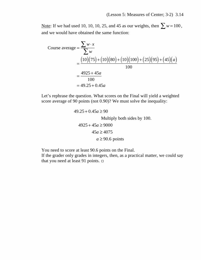
Note: If we had used 10, 10, 10, 25, and 45 as our weights, then
w = 100 ,
and we would have obtained the same function:
Course average =w x
w
=10( ) 75( ) + 10( ) 80( ) + 10( ) 100( ) + 25( ) 95( ) + 45( ) a( )
100
=4925+ 45a
100
= 49.25+ 0.45a
Let’s rephrase the question. What scores on the Final will yield a weighted
score average of 90 points (not 0.90)? We must solve the inequality:
49.25+ 0.45a 90
Multiply both sides by 100.
4925+ 45a 9000
45a 4075
a 90.6 points
You need to score at least 90.6 points on the Final.
If the grader only grades in integers, then, as a practical matter, we could say
that you need at least 91 points.

(Lesson 6: Measures of Spread or Variation; 3-3) 3.15
LESSON 6: MEASURES OF SPREAD OR VARIATION(SECTION 3-3)
PART A: THREE MEASURES
Example 1 (same as in Lesson 5)
The five students in a class take a test. Their scores in points are as follows:
80 76 100 83 100
Let’s look at three possibilities for measuring the spread or variation of adata set.
Note: All three of these measures are nonnegative in value.
1) Range
Range = Max − Min
= highest value − lowest value in the data set( )In Example 1
Range = Max − Min
= 100 − 76
= 24 points
Pros: The range is quick and easy to find, and it seems like a natural measureof spread.
Cons: The range uses only two of the data values (excluding ties), and it isextremely sensitive to outliers.
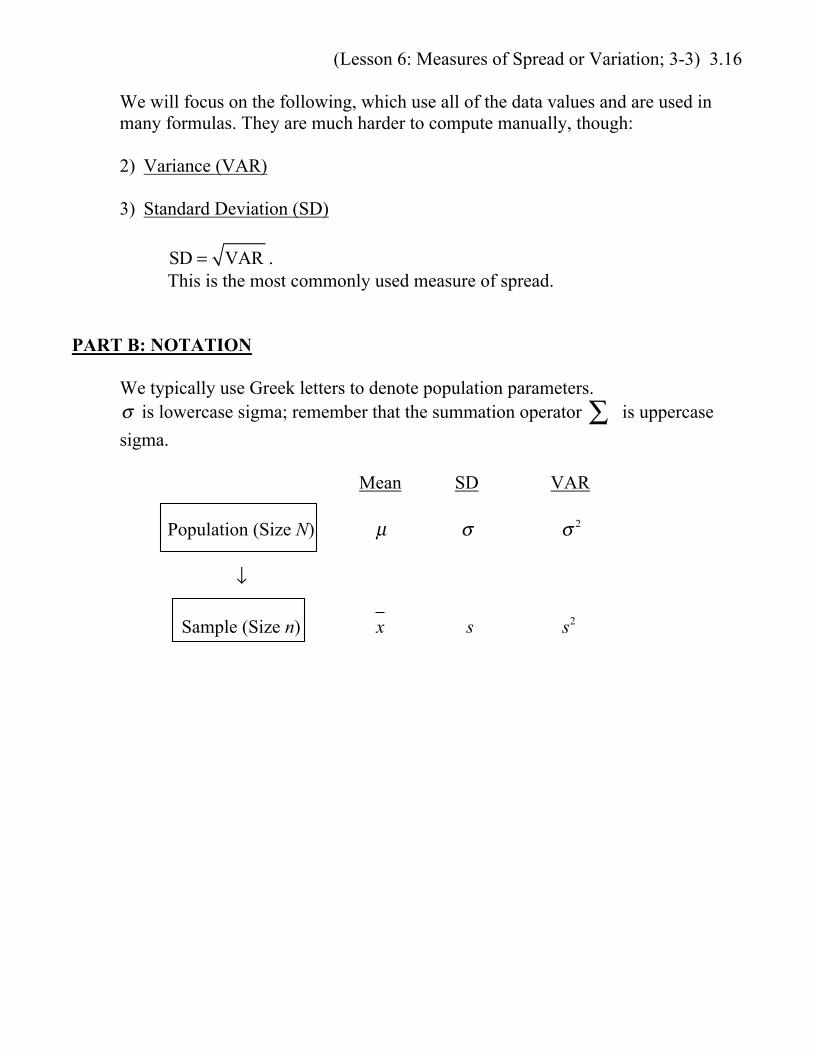
(Lesson 6: Measures of Spread or Variation; 3-3) 3.16
We will focus on the following, which use all of the data values and are used inmany formulas. They are much harder to compute manually, though:
2) Variance (VAR)
3) Standard Deviation (SD)
SD = VAR .This is the most commonly used measure of spread.
PART B: NOTATION
We typically use Greek letters to denote population parameters.σ is lowercase sigma; remember that the summation operator ∑ is uppercase
sigma.
Mean SD VAR
Population (Size N) µ σ σ 2
↓
Sample (Size n) x s s2

(Lesson 6: Measures of Spread or Variation; 3-3) 3.17
PART C: POPULATION DATA
What are the population variance, σ 2 , and the population standard deviation, σ , ofa population data set?
Idea
Focus on the mean as a reference point; envision planting a flag there on thereal number line. We want to measure the spread of the data values aroundthe mean.
Let’s compare another pair of data sets using the same scale:
(Lesson 6: Measures of Spread or Variation; 3-3) 3.18
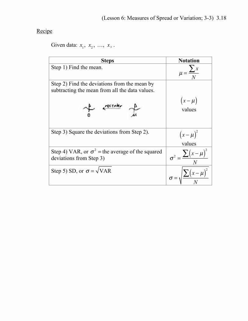
Recipe
Given data: x
1, x
2, …, xN .
Steps NotationStep 1) Find the mean.
µ =
x∑N
Step 2) Find the deviations from the mean bysubtracting the mean from all the data values.
x − µ( )
values
Step 3) Square the deviations from Step 2).
x − µ( )2
valuesStep 4) VAR, or σ 2 = the average of the squareddeviations from Step 3)
σ 2 =
x − µ( )2∑N
Step 5) SD, or σ = VAR
σ =
x − µ( )2∑N

(Lesson 6: Measures of Spread or Variation; 3-3) 3.19
Back to Example 1
Find the population VAR and SD of the given data set.
Show all work on exams!
Data
x( )
Step 2Deviations:
x − µ( ) values
Step 3Squared Deviations:
x − µ( )2
values
80 − 7.8 60.8476 − 11.8 139.24
100 12.2 148.8483 − 4.8 23.04
100 12.2 148.84Step 1:
µ = 87.8points
See Note 2below.
Sum = 520.8
Do Steps 4, 5.
Note 1: You should fill out the above table row by row. For example, takethe “80”, subtract off the mean, and then square the result:
80 Subtract 87.8⎯ →⎯⎯⎯ −7.8 Square⎯ →⎯⎯ 60.84
Note 2: Why not use the sum or average of the deviations as a measure ofspread? It is always 0 for any data set, so it is meaningless as a measure ofspread. The deviations effectively cancel each other out. This reflects thefact that the new mean of our recentered data set is 0. For this and for othertheoretical reasons, we square the deviations before taking an average. Whatif we were to take the absolute values of the deviations before taking anaverage? The result would be the mean absolute deviation (MAD), which isdiscussed on pp.102-103 of Triola.
Note 3 on Rounding: We were fortunate that exact values were easilywritten in the table. See Notes 3.02 for a reminder of our rounding rules forChapter 3.
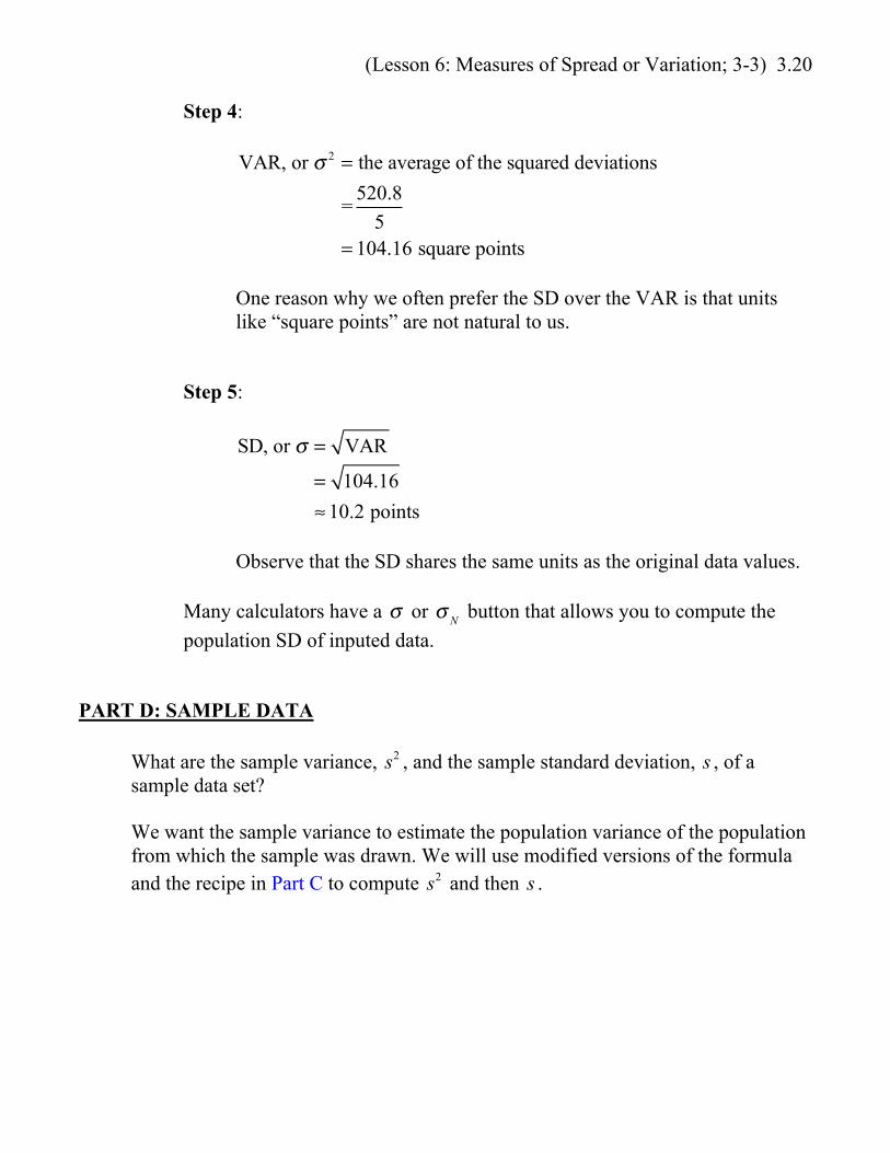
(Lesson 6: Measures of Spread or Variation; 3-3) 3.20
Step 4:
VAR, or σ 2 = the average of the squared deviations
=520.8
5= 104.16 square points
One reason why we often prefer the SD over the VAR is that unitslike “square points” are not natural to us.
Step 5:
SD, or σ = VAR
= 104.16
≈ 10.2 points
Observe that the SD shares the same units as the original data values.
Many calculators have a σ or σ N button that allows you to compute the
population SD of inputed data.
PART D: SAMPLE DATA
What are the sample variance, s2 , and the sample standard deviation, s , of a
sample data set?
We want the sample variance to estimate the population variance of the populationfrom which the sample was drawn. We will use modified versions of the formulaand the recipe in Part C to compute s
2 and then s .

(Lesson 6: Measures of Spread or Variation; 3-3) 3.21
Mean SD VAR
Population (Size N) µ σ σ 2
↓
Sample (Size n) x s s2
The formula for sample variance is given by:
s2 =
x − x( )2
∑n −1
The formula for sample SD is then given by:
s =
x − x( )2
∑n −1
Note 1: How does this differ from the formula for σ ? The population mean,
µ , is presumably unknown, so we replace it with the sample mean, x . Wealso replace the population size, N, with n −1. But ….
Note 2: Why n −1, not n? Why is s the square root of a “tilted” average of
the squared deviations from the sample mean, x ? The appropriate reference
point is still the population mean, µ , not x . The sample data values aremore naturally clustered around their sample mean than around thepopulation mean. In order to make s
2 a better estimate for σ 2 , thepopulation variance, we inflate our estimate by dividing by n −1 instead of
n.
Remember, for example: 1
4>
1
5
⎛⎝⎜
⎞⎠⎟
. Then, s2 will be an unbiased estimator
of σ 2 in that it does not have an automatic tendency to consistently over- orunderestimate σ 2 .

(Lesson 6: Measures of Spread or Variation; 3-3) 3.22
Note 3: Triola on p.94 provides the following alternate formula, which ismuch harder to remember but is more often used in computers andcalculators:
s =n x2( )∑ − x∑( )2
n n −1( )This formula is algebraically equivalent to the previous one. It is a one-passformula in that a computer or calculator does not need to use the data valuesmore than once. In particular, the sample mean does not have to becomputed first. (The previous formula is a two-pass formula.) This latterformula is preferred for maximum accuracy in that it does more to avoidroundoff errors.
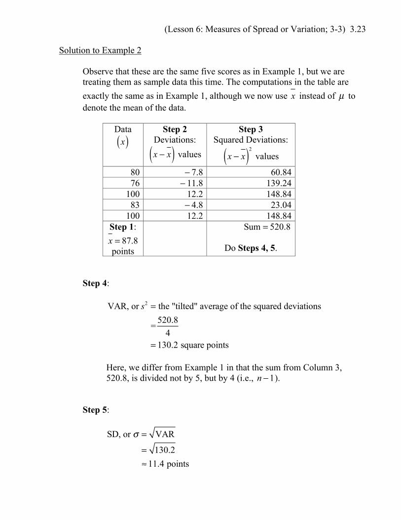
Example 2
We will modify Example 1. Let’s say 1000 students in a large lecture classhave taken a test. Five of the tests are randomly selected, and their scores areas follows:
80 76 100 83 100
Find the sample VAR and SD of the given data set.
Population (Size 1000)
↓
Sample (Size 5)
(Lesson 6: Measures of Spread or Variation; 3-3) 3.23
Solution to Example 2
Observe that these are the same five scores as in Example 1, but we aretreating them as sample data this time. The computations in the table are
exactly the same as in Example 1, although we now use x instead of µ todenote the mean of the data.
Data
x( )
Step 2Deviations:
x − x( ) values
Step 3Squared Deviations:
x − x( )2
values
80 − 7.8 60.8476 − 11.8 139.24
100 12.2 148.8483 − 4.8 23.04
100 12.2 148.84Step 1:
x = 87.8points
Sum = 520.8
Do Steps 4, 5.
Step 4:
VAR, or s2 = the "tilted" average of the squared deviations
=520.8
4= 130.2 square points
Here, we differ from Example 1 in that the sum from Column 3,520.8, is divided not by 5, but by 4 (i.e., n −1).
Step 5:
SD, or σ = VAR
= 130.2
≈ 11.4 points
(Lesson 6: Measures of Spread or Variation; 3-3) 3.24
Observe that this is higher than 10.2 points, the SD from Example 1.The “tilted” average we used in Step 4 inflated our value for thesample SD.
Many calculators have an s or σ n−1 button that allows you to compute the sample
SD of inputed data.
PART E: APPLICATIONS
If the population SD of a data set is 10.2 points, what is the usefulness of that?
If we have different populations (for example, men and women) for which thesame measure (such as age or height using the same units) is being taken, then wecould compare their SDs.
In Parts F, G, and H, we will use the SD to provide information about how datavalues are distributed. To avoid confusion, let’s say we’re dealing with thepopulation SD of a population data set.
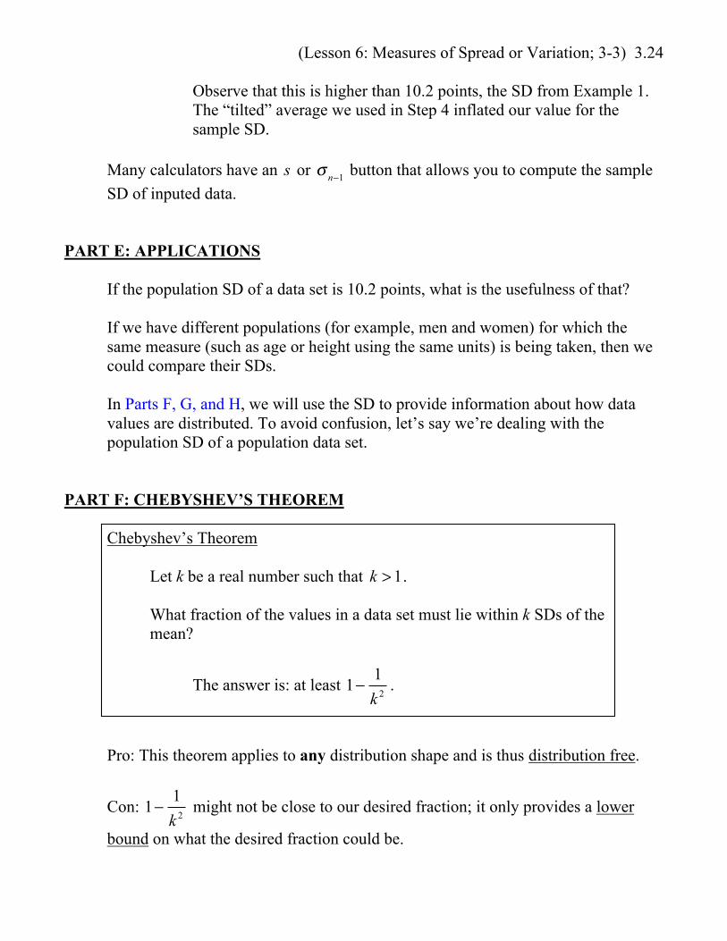
PART F: CHEBYSHEV’S THEOREM
Chebyshev’s Theorem
Let k be a real number such that k > 1.
What fraction of the values in a data set must lie within k SDs of themean?
The answer is: at least 1−
1
k 2.
Pro: This theorem applies to any distribution shape and is thus distribution free.
Con: 1−
1
k 2 might not be close to our desired fraction; it only provides a lower
bound on what the desired fraction could be.
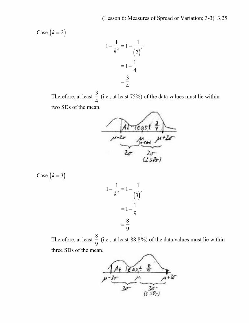
(Lesson 6: Measures of Spread or Variation; 3-3) 3.25
Case k = 2( )
1−1
k 2= 1−
1
2( )2
= 1−1
4
=3
4
Therefore, at least
3
4 (i.e., at least 75%) of the data values must lie within
two SDs of the mean.
Case k = 3( )
1−1
k 2= 1−
1
3( )2
= 1−1
9
=8
9
Therefore, at least
8
9 (i.e., at least 88.8%) of the data values must lie within
three SDs of the mean.

(Lesson 6: Measures of Spread or Variation; 3-3) 3.26
Example 3
The scores on a test have mean µ = 50 points and SD σ = 10 points .
By Chebyshev’s Theorem:
At least
3
4 of the test scores are between 30 points and 70 points.
At least
8
9 of the test scores are between 20 points and 80 points.
PART G: 68-95-99.7 EMPIRICAL RULE FOR APPROXIMATELY NORMALDATA
In practice (i.e., “Empirically”), we often see distributions that are approximatelynormal. Normal distributions are an important class of bell shaped distributionsthat we will revisit in Chapter 6.
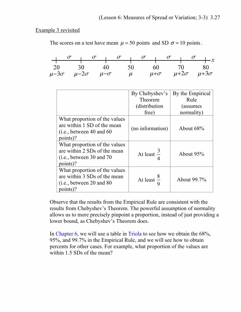
(Lesson 6: Measures of Spread or Variation; 3-3) 3.27
Example 3 revisited
The scores on a test have mean µ = 50 points and SD σ = 10 points .
By Chebyshev’sTheorem
(distributionfree)
By the EmpiricalRule
(assumesnormality)
What proportion of the valuesare within 1 SD of the mean(i.e., between 40 and 60points)?
(no information) About 68%
What proportion of the valuesare within 2 SDs of the mean(i.e., between 30 and 70points)?
At least
3
4About 95%
What proportion of the valuesare within 3 SDs of the mean(i.e., between 20 and 80points)?
At least
8
9About 99.7%
Observe that the results from the Empirical Rule are consistent with theresults from Chebyshev’s Theorem. The powerful assumption of normalityallows us to more precisely pinpoint a proportion, instead of just providing alower bound, as Chebyshev’s Theorem does.
In Chapter 6, we will use a table in Triola to see how we obtain the 68%,95%, and 99.7% in the Empirical Rule, and we will see how to obtainpercents for other cases. For example, what proportion of the values arewithin 1.5 SDs of the mean?

(Lesson 6: Measures of Spread or Variation; 3-3) 3.28
PART H: RANGE RULE OF THUMB
Both Chebyshev’s Theorem and the Empirical Rule imply that, in terms of SDs,we can’t have too much of the data too far away from the mean. In particular, the“vast majority” of the data must lie within two SDs of the mean. (We could alsouse three SDs, for example.)
Range Rule of Thumb for Interpreting σ
The vast majority of the values in a population data set will lie between
µ − 2σ and µ + 2σ .
Example 3 revisited
The scores on a test have mean µ = 50 points and SD σ = 10 points .
The “vast majority” of the scores must lie between 30 and 70 points.
Let’s say that the “realistic range” of the data set is 70 − 30 = 40 points .The idea is that few of the scores will be less than 30 points or greater than70 points.
In general, Realistic range ≈ 4σ . As a result, we obtain:
Range Rule of Thumb for Estimating σ
σ ≈
Realistic range
4

(Lesson 6: Measures of Spread or Variation; 3-3) 3.29
Example 4
We believe that the “vast majority” of textbooks in a campus bookstore haveprices between $20 and $180. Estimate σ , the SD of textbook prices in thebookstore.
Solution to Example 4
σ ≈Realistic range
4
σ ≈$180 − $20
4
σ ≈$160
4σ ≈ $40
Again, this is a very rough estimate. We at least expect it to be on the correctorder of magnitude, as opposed to, say, $4 or $400.
PART I: INVESTING
The benefit of a diverse portfolio is that risk is spread out across many stocks.No single stock will destroy you. Your hope is that your stock portfolio will atleast keep up with the general upward trend of the market over time.
See the margin essay “More Stocks, Less Risk” on p.99.

(Lesson 7: Measures of Relative Standing or Position; 3-4) 3.30
LESSON 7: MEASURES OF RELATIVE STANDING OR
POSITION (SECTION 3-4)
How high or low is a data value relative to the others? We want standardized measures
that will work for practically all populations involving quantitative data.
PART A: z SCORES
z =x mean
SDIdea:
new mean = 0
new SD = 1
We are transforming the original data set of x-values into a new data set of
z-values.
x1
x2
x3
etc.
z1
z2
z3
etc.
Subtracting off the mean from all of the original x-values recenters the data
set so that the new mean will be 0. Then, dividing by the SD rescales the
data set so that the new SD will be 1.
Notation
Population (Size N)
z =x μ
Sample (Size n) z =x x
s
Round off z scores to two decimal places.
They have no units, because we divide by the SD. We will be able to use z scores
in many different applications where different units are involved. If we are
studying heights, for instance, we may use inches, feet, meters, etc. and still obtain
the same z scores.

(Lesson 7: Measures of Relative Standing or Position; 3-4) 3.31
z Score Rule of Thumb for “Unusual” Data Values
Data values whose corresponding z scores are either less than 2 or greater
than 2 (i.e., z < 2 or z > 2 ) are often considered “unusual.”
In other words, data values that are more than 2 SDs from the mean are
often considered “unusual.”
Think About It: How would you feel if your instructor tells you that your z score
for the test you just took was 2.31?
Example
Two statistics classes take different tests.
The mean and SD for Class 1 are: μ
1= 55 points ,
1= 5 points .
The mean and SD for Class 2 are: μ2= 60 points ,
2= 10 points .
In which class is a score of 70 points more impressive?
Solution
Find the corresponding z scores for 70 points in the two classes.
Class 1: Class 2:
z =70 55
5
= 3.00
z =
70 60
10
= 1.00
A score of 70 points is more impressive in Class 1; in fact, it is “unusually”
high in that class.

(Lesson 7: Measures of Relative Standing or Position; 3-4) 3.32
Note: If we assume normality in both classes, we have:
PART B: FRACTILES, OR QUANTILES
We will look at three types of these.
Percentiles
Example
Because 92% of the scores lie below 85 points, we can say that the
92nd
percentile of the data is 85: P
92= 85 points .
(Lesson 7: Measures of Relative Standing or Position; 3-4) 3.33
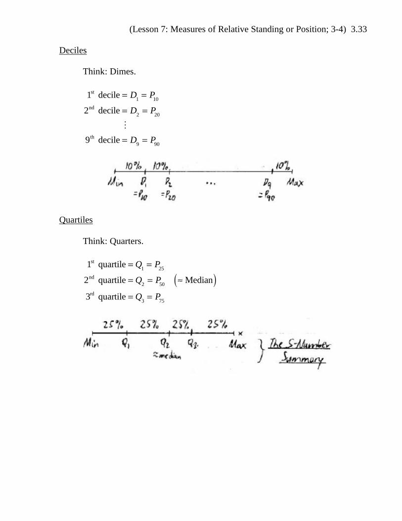
Deciles
Think: Dimes.
1st decile = D1= P
10
2nd decile = D2= P
20
9th decile = D9= P
90
Quartiles
Think: Quarters.
1st quartile = Q1= P
25
2nd quartile = Q2= P
50Median( )
3rd quartile = Q3= P
75

(Lesson 8: Boxplots; also 3-4) 3.34
LESSON 8: BOXPLOTS (ALSO SECTION 3-4)
The Five-Number Summary can be represented graphically as a boxplot, or box-and-
whisker plot.
Boxplots can help us compare different populations, such as men and women.
See the last page of the MINITAB handout.
(Lesson 9: Probability Basics; 4-2) 4.01
CHAPTER 4: PROBABILITY
The French mathematician Laplace once claimed that probability theory is nothing but“common sense reduced to calculation.” This is true many times, but not always ….
LESSON 9: PROBABILITY BASICS (SECTION 4-2)
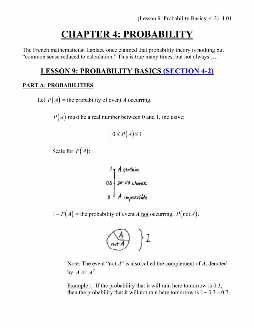
PART A: PROBABILITIES
Let P A( ) = the probability of event A occurring.
P A( ) must be a real number between 0 and 1, inclusive:
0 ≤ P A( ) ≤ 1
Scale for P A( ) :
1− P A( ) = the probability of event A not occurring,
P not A( ) .
Note: The event “not A” is also called the complement of A, denoted
by A or AC .
Example 1: If the probability that it will rain here tomorrow is 0.3,then the probability that it will not rain here tomorrow is 1− 0.3= 0.7 .

(Lesson 9: Probability Basics; 4-2) 4.02
PART B: ROUNDING
Rounding conventions may be inconsistent.
Triola suggests either writing probabilities exactly, such as
1
3, or rounding off to
three significant digits, such as 0.333 (33.3%) or 0.00703 (0.703%). Althoughthere is some controversy about the use of percents as probabilities, we willsometimes use percents. Remember that “leading zeros” don’t count whencounting significant digits. It is true that 0.00703 has five decimal places.
If your final answers are rounded off to, say, three significant digits, thenintermediate results should be either exact or rounded off to more significant digits(at least twice as many, six, perhaps).
Note: If a probability is close to 1, such as 0.9999987, or if it is close to anotherprobability in a given problem, then you may want to use more than threesignificant digits.
Always read any instructions in class.
PART C: THREE APPROACHES TO PROBABILITY
Approach 1): Classical Approach
Assume that a trial (such as rolling a die, flipping a fair coin, etc.) mustresult in exactly one of N equally likely outcomes (we’ll say “elos”) that aresimple events, which can’t really be broken down further.
The elos make up the sample space, S.
Then, P A( ) = # of elos for which A occurs
N.

(Lesson 9: Probability Basics; 4-2) 4.03
Example 2 (Roll One Die)
We roll one standard six-sided die.
S = 1, 2, 3, 4, 5, 6{ }.
N = 6 elos.
Notation: We will use shorthand. For example, the event “4” means“the die comes up ‘4’ when it is rolled.” It is a simple event.
P 4( ) = 1
6.
The odds against the event happening are 5 to 1.
P even( ) = 3
6
=1
2
“Even” is a compound event, because it combines two or moresimple events.

(Lesson 9: Probability Basics; 4-2) 4.04
Example 3 (Roll Two Dice – 1 red, 1 green)
We roll two standard six-sided dice.
It turns out to be far more convenient if we distinguish between thedice. For example, we can color one die red and the other die green.
Think About It: Are dice totals equally likely?
Our simple events are ordered pairs of the form r, g( ) , where r is the
result on the red die and g is the result on the green die.
S = 1,1( ) , 1, 2( ) ,…, 6, 6( ){ }.
N = 36 elos.
Notation: We will use shorthand. For example, the event “4” means“the die comes up ‘4’ when it is rolled.” It is a simple event.
P 4, 2( )( ) = 1
36
P 2 on red( ) = 6
36
=1
6
Think About It: Why does this answer make sense? How couldyou have answered very quickly?
(Lesson 9: Probability Basics; 4-2) 4.05
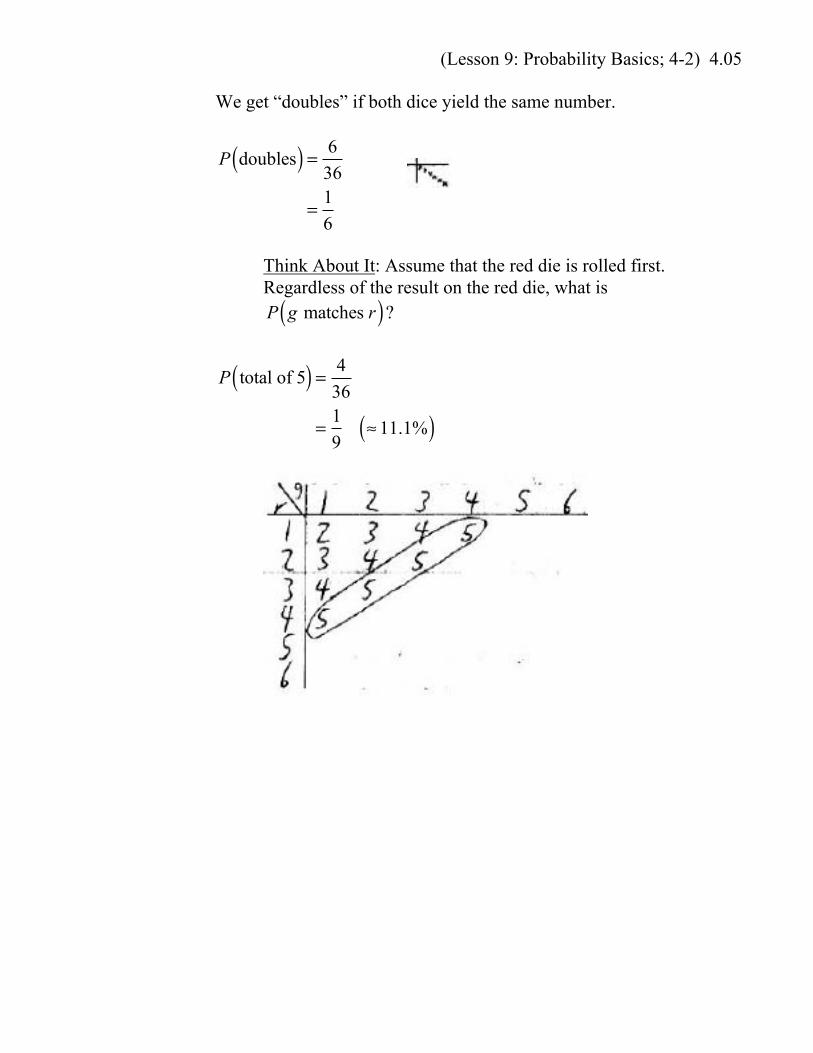
We get “doubles” if both dice yield the same number.
P doubles( ) = 6
36
=1
6
Think About It: Assume that the red die is rolled first.Regardless of the result on the red die, what is
P g matches r( )?
P total of 5( ) = 4
36
=1
9≈ 11.1%( )

(Lesson 9: Probability Basics; 4-2) 4.06
Example 4 (Roulette)
18 red slots P red( ) = 18
38=
9
19≈ 47.4%( )
18 black slots P black( ) = 18
38=
9
19≈ 47.4%( )
2 green slots P green( ) = 2
38=
1
19≈ 5.26%( )
38 total
The casino pays “even money” for red / black bets; in other words,every dollar bet is matched by the casino if the player wins. This isslightly unfair to the player! A fair payoff would be about $1.11 forevery dollar bet. But then, the casino wouldn’t be making a profit!
According to the Law of Large Numbers (LLN), the probabilities builtinto the game will “crystallize” in the long run. In other words, theobserved relative frequencies of red, black, and green results willapproach the corresponding theoretical probabilities
9
19,
9
19, and
1
19
⎛⎝⎜
⎞⎠⎟
after many bets. In the long run, on average, the
casino will make a profit of about 5.26 cents for every dollar bet byplayers in red / black bets. We say that the house advantage is 5.26%;see the margin essay “You Bet” on p.140.
How do you maximize your chances of winning a huge amount ofmoney?
(Lesson 9: Probability Basics; 4-2) 4.07
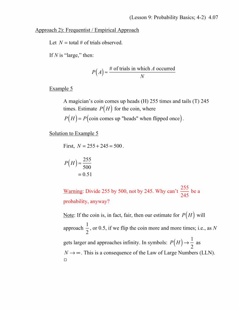
Approach 2): Frequentist / Empirical Approach
Let N = total # of trials observed.
If N is “large,” then:
P A( ) ≈ # of trials in which A occurred
N
Example 5
A magician’s coin comes up heads (H) 255 times and tails (T) 245times. Estimate
P H( ) for the coin, where
P H( ) = P coin comes up "heads" when flipped once( ) .
Solution to Example 5
First, N = 255+ 245 = 500 .
P H( ) ≈ 255
500= 0.51
Warning: Divide 255 by 500, not by 245. Why can’t
255
245 be a
probability, anyway?
Note: If the coin is, in fact, fair, then our estimate for P H( ) will
approach
1
2, or 0.5, if we flip the coin more and more times; i.e., as N
gets larger and approaches infinity. In symbols: P H( )→ 1
2 as
N →∞ . This is a consequence of the Law of Large Numbers (LLN).
(Lesson 9: Probability Basics; 4-2) 4.08
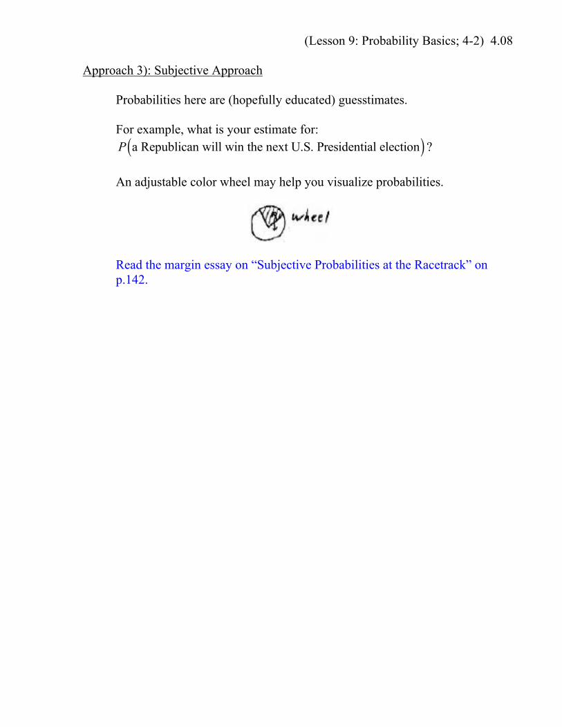
Approach 3): Subjective Approach
Probabilities here are (hopefully educated) guesstimates.
For example, what is your estimate for:
P a Republican will win the next U.S. Presidential election( ) ?
An adjustable color wheel may help you visualize probabilities.
Read the margin essay on “Subjective Probabilities at the Racetrack” onp.142.
(Lesson 10: Addition Rule; 4-3) 4.09
LESSON 10: ADDITION RULE (SECTION 4-3)
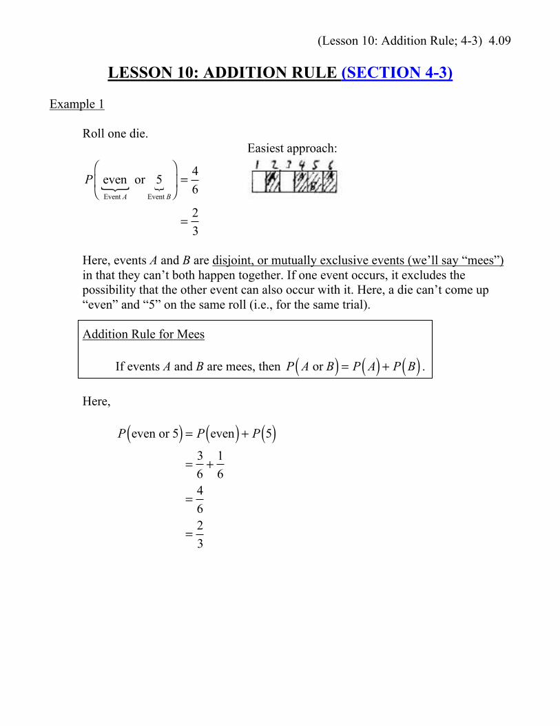
Example 1
Roll one die.Easiest approach:
P evenEvent A or 5
Event B
⎛
⎝⎜
⎞
⎠⎟ =
4
6
=2
3
Here, events A and B are disjoint, or mutually exclusive events (we’ll say “mees”)in that they can’t both happen together. If one event occurs, it excludes thepossibility that the other event can also occur with it. Here, a die can’t come up“even” and “5” on the same roll (i.e., for the same trial).
Addition Rule for Mees
If events A and B are mees, then P A or B( ) = P A( ) + P B( ) .
Here,
P even or 5( ) = P even( ) + P 5( )=
3
6+
1
6
=4
6
=2
3
(Lesson 10: Addition Rule; 4-3) 4.10
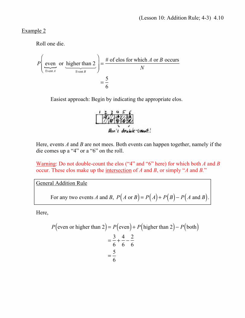
Example 2
Roll one die.
P evenEvent A or higher than 2
Event B
⎛
⎝⎜⎜
⎞
⎠⎟⎟=
# of elos for which A or B occurs
N
=5
6
Easiest approach: Begin by indicating the appropriate elos.
Here, events A and B are not mees. Both events can happen together, namely if thedie comes up a “4” or a “6” on the roll.
Warning: Do not double-count the elos (“4” and “6” here) for which both A and Boccur. These elos make up the intersection of A and B, or simply “A and B.”
General Addition Rule
For any two events A and B, P A or B( ) = P A( ) + P B( ) − P A and B( ) .
Here,
P even or higher than 2( ) = P even( ) + P higher than 2( ) − P both( )=
3
6+
4
6−
2
6
=5
6
(Lesson 10: Addition Rule; 4-3) 4.11
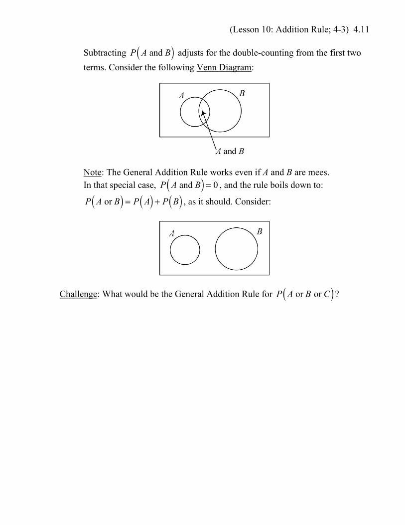
Subtracting P A and B( ) adjusts for the double-counting from the first two
terms. Consider the following Venn Diagram:
Note: The General Addition Rule works even if A and B are mees.In that special case,
P A and B( ) = 0 , and the rule boils down to:
P A or B( ) = P A( ) + P B( ) , as it should. Consider:
Challenge: What would be the General Addition Rule for P A or B or C( )?

(Lesson 10: Addition Rule; 4-3) 4.12
Example 3
Roll two dice.
P doubles or a "6" on either die( ) = 16
36
=4
9≈ 44.4%( )
A formula would be tricky to apply here. We’ll use a diagram, instead.
Example 4
All 26 students in a class are passing, but they seek tutoring. One tutor is a Juniorwho likes helping students who are Juniors or who are receiving a “B” or a “C”.Based on the following two-way frequency (or contingency) table, find
P a random student in the class is a Junior or is getting a "B" or a "C"( ) .
A B CSophomores 1 0 2
Juniors 5 8 1Seniors 2 4 3
(Lesson 10: Addition Rule; 4-3) 4.13
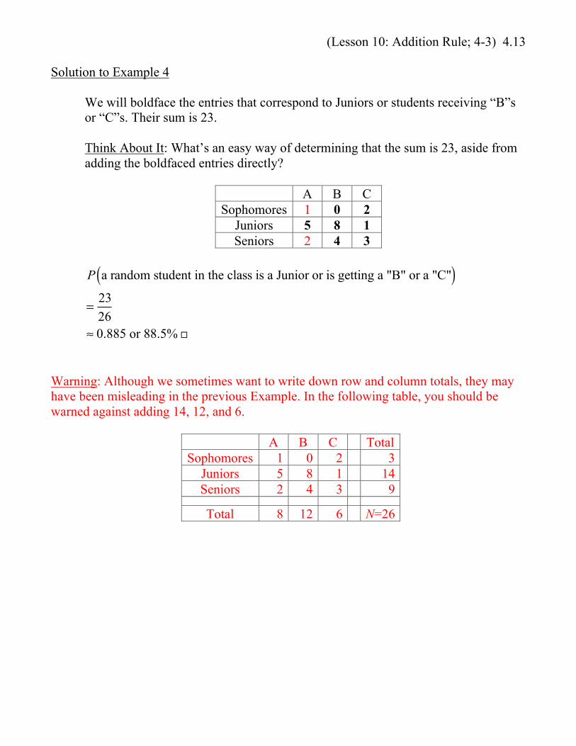
Solution to Example 4
We will boldface the entries that correspond to Juniors or students receiving “B”sor “C”s. Their sum is 23.
Think About It: What’s an easy way of determining that the sum is 23, aside fromadding the boldfaced entries directly?
A B CSophomores 1 0 2
Juniors 5 8 1Seniors 2 4 3
P a random student in the class is a Junior or is getting a "B" or a "C"( )=
23
26≈ 0.885 or 88.5%
Warning: Although we sometimes want to write down row and column totals, they mayhave been misleading in the previous Example. In the following table, you should bewarned against adding 14, 12, and 6.
A B C TotalSophomores 1 0 2 3
Juniors 5 8 1 14Seniors 2 4 3 9
Total 8 12 6 N=26

(Lesson 11: Multiplication Rule; 4-4) 4.14
LESSON 11: MULTIPLICATION RULE (SECTION 4-4)
PART A: INDEPENDENT EVENTS
Example 1
Pick (or “draw”) a card from a standard deck of 52 cards with no Jokers.(Know this setup!)
P 3( ) = 4
52=
1
13(The 13 ranks are equally likely.)
P hearts( ) = 13
52=
1
4(The 4 suits are equally likely.)
P 3 and hearts( ) = 1
52(The 52 cards are equally likely.)
(Lesson 11: Multiplication Rule; 4-4) 4.15
The events “3” and “Hearts” are independent events, because knowing therank of a card tells us nothing about its suit, and vice-versa. The occurrenceof one event does not change our probability assessment for the other event.The rank and the suit of an unknown card are independent random variables,which we will discuss later.
Dependent events are events that are not independent.
Multiplication Rule for Independent Events
If events A, B, C, etc. are independent, then:
P A and B( ) = P A( ) ⋅ P B( ) P A and B and C( ) = P A( ) ⋅ P B( ) ⋅ P C( ) , etc.
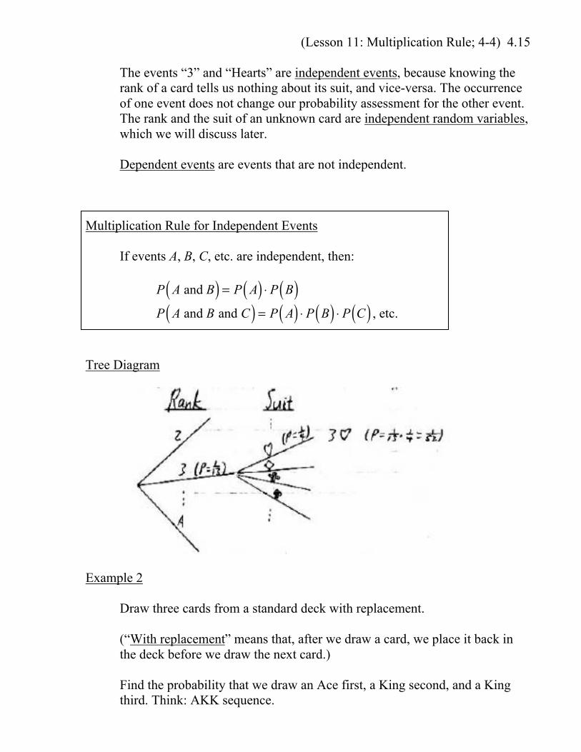
Tree Diagram
Example 2
Draw three cards from a standard deck with replacement.
(“With replacement” means that, after we draw a card, we place it back inthe deck before we draw the next card.)
Find the probability that we draw an Ace first, a King second, and a Kingthird. Think: AKK sequence.
(Lesson 11: Multiplication Rule; 4-4) 4.16
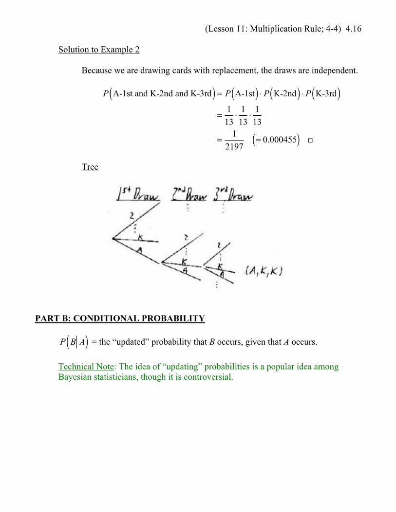
Solution to Example 2
Because we are drawing cards with replacement, the draws are independent.
P A-1st and K-2nd and K-3rd( ) = P A-1st( ) ⋅ P K-2nd( ) ⋅ P K-3rd( )=
1
13⋅
1
13⋅
1
13
=1
2197≈ 0.000455( )
Tree
PART B: CONDITIONAL PROBABILITY
P B A( ) = the “updated” probability that B occurs, given that A occurs.
Technical Note: The idea of “updating” probabilities is a popular idea amongBayesian statisticians, though it is controversial.
(Lesson 11: Multiplication Rule; 4-4) 4.17
PART C: DEPENDENT EVENTS
P B A( ) = the “updated” probability that B occurs, given that A occurs.
General Multiplication Rule
For events A, B, C, etc.,
P A and B( ) = P A( ) ⋅ P B A( ) P A and B and C( ) = P A( ) ⋅ P B A( ) ⋅ P C A and B( ) , etc.
Note: If A and B are independent, then the occurrence of A does not change
our probability assessment for B, and P B A( ) = P B( ) . In that case, the
General Multiplication Rule becomes the Multiplication Rule forIndependent Events that we discussed earlier:
P A and B( ) = P A( ) ⋅ P B( ) .
Example 3
Draw three cards from a standard deck without replacement.
(“Without replacement” means that drawn cards are never returned back tothe deck.)
Find the probability that we draw an Ace first, a King second, and a Kingthird. Think: AKK sequence.
(Lesson 11: Multiplication Rule; 4-4) 4.18
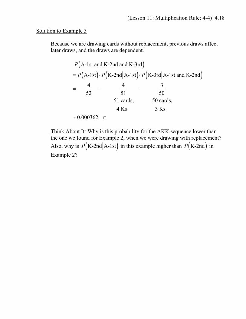
Solution to Example 3
Because we are drawing cards without replacement, previous draws affectlater draws, and the draws are dependent.
P A-1st and K-2nd and K-3rd( )= P A-1st( ) ⋅ P K-2nd A-1st( ) ⋅ P K-3rd A-1st and K-2nd( )=
4
52⋅
4
51⋅
3
50 51 cards, 50 cards,
4 Ks 3 Ks
≈ 0.000362
Think About It: Why is this probability for the AKK sequence lower thanthe one we found for Example 2, when we were drawing with replacement?
Also, why is P K-2nd A-1st( ) in this example higher than
P K-2nd( ) in
Example 2?

(Lesson 11: Multiplication Rule; 4-4) 4.19
PART D: SAMPLING RULE FOR TREATING DEPENDENT EVENTS ASINDEPENDENT
When we conduct polls, we sample without replacement, so that the same person isnot contacted twice. Technically, the selections are dependent.
Sometimes, to simplify our calculations, we can treat dependent events asindependent, and our results will still be reasonably accurate. We can do this whenwe take relatively small samples from large populations; then, we can practicallyassume that we are sampling with replacement, and we can ignore the unlikelypossibility of the same item (or person) being selected twice.
Sampling Rule for Treating Dependent Events as Independent
Population (Size N) ( N ≥ 1000 , say)
↓ (even if we draw without replacement)
Sample (Size n) ( n ≤ 0.05N )
If we are drawing a sample of size n from a population of size N withoutreplacement, then, even though the selections are dependent, we canpractically treat them as independent if:
• The sample size is no more than 5% of the population size:
n ≤ 5% of N( ) , or n ≤ 0.05N ,
and
• The population size, N, is large: say, for our class, N ≥ 1000 .

(Lesson 11: Multiplication Rule; 4-4) 4.20
Example 4
G.W. Bush won 47.8% of the popular vote in 2000.(Al Gore won 48.4%, and Ralph Nader won 2.7%.)Over 105 million voters in the U.S. voted for President in 2000.Of those, three are randomly selected without replacement.Find the probability that all three selected voters voted for Bush in 2000.
Solution to Example 4
Observe that we are sampling no more than 5% of a huge population.By the aforementioned Sampling Rule, we may practically assume that theselections are independent.
Since Bush won 47.8% of the vote, the probability that a randomly selectedvoter voted for Bush is 47.8%, or 0.478.
Warning: Avoid using percents when doing calculations.
P all three selected voters voted for Bush( )= P 1st-Bush( ) ⋅ P 2nd-Bush( ) ⋅ P 3rd-Bush( )= 0.478( ) 0.478( ) 0.478( ) , or 0.478( )3
≈ 0.109 or 10.9%( )
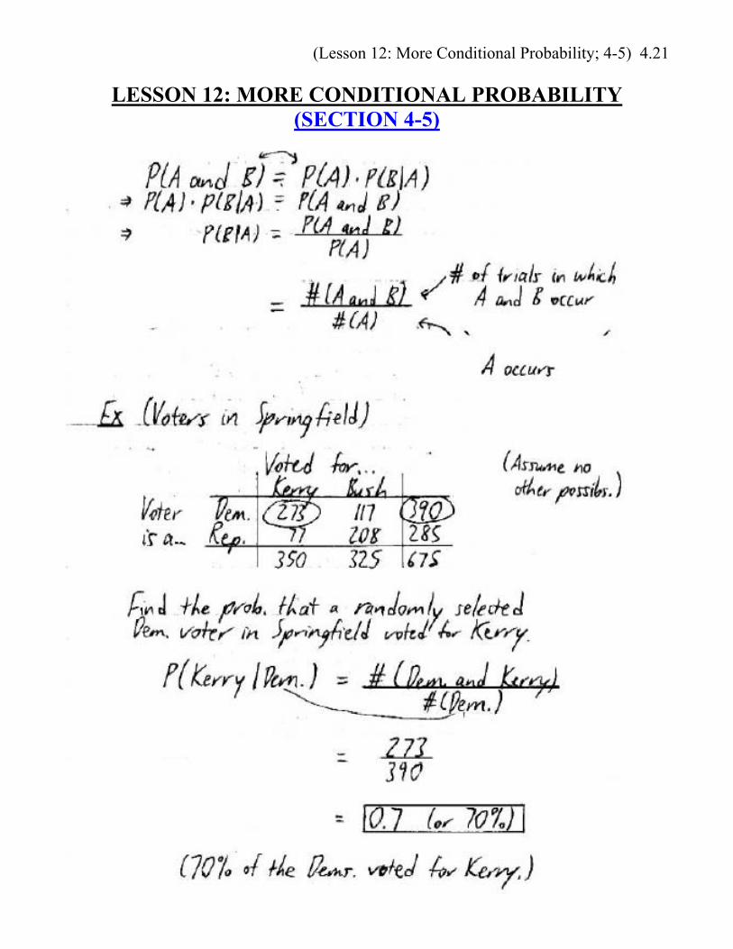
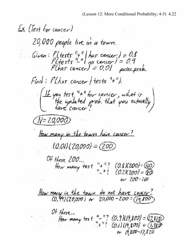
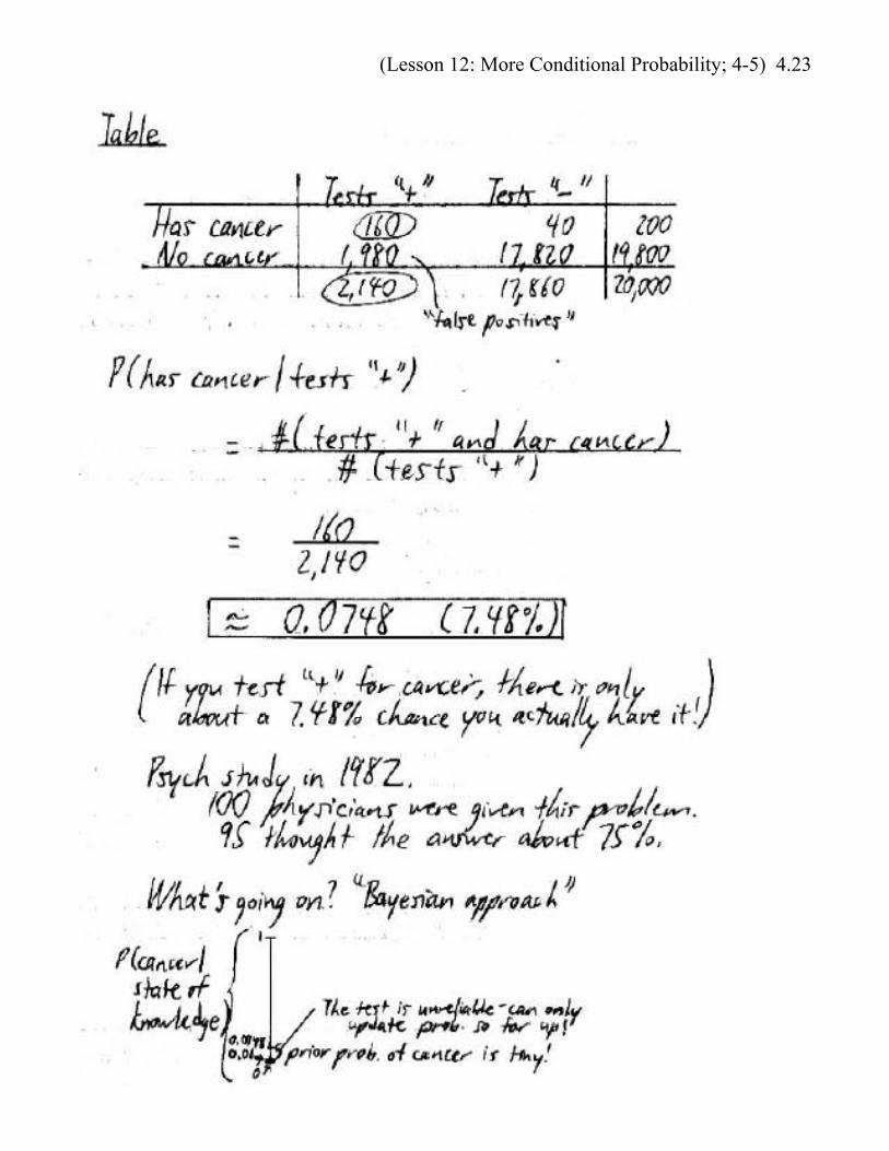
(Lesson 12: More Conditional Probability; 4-5) 4.21
LESSON 12: MORE CONDITIONAL PROBABILITY(SECTION 4-5)
(Lesson 12: More Conditional Probability; 4-5) 4.22
(Lesson 12: More Conditional Probability; 4-5) 4.23

(Lesson 12: More Conditional Probability; 4-5) 4.24