Chapter 1

Introduction

Computers on the Internet communicate with each other by passing messages dividedinto units called packets. Since each computer does not have wires connecting it to everyother computer on the Internet, packets are passed along from source to destination throughintermediate computers, called routers. Each packet contains the address of the source anddestination so that the routers know where to send the packet and so the destination knowswho sent the packet. When packets arrive at a router faster than they can be processedand forwarded, the router saves the incoming packets into a queue. Network congestionresults when the number of packets in this queue remains large for a sustained period oftime. The longer the queue, the longer that packets at the end of the queue must wait beforebeing transferred, thus, increasing their delay. Network congestion can cause the queueto completely fill. When this occurs, incoming packets are dropped and never reach theirdestination. Protocols that control transport of data, such as TCP, must handle these packetloss situations.

This dissertation is concerned with detecting and reacting to network congestion beforepackets are dropped, and thus, improving performance for Internet applications, such as email,file transfer, and browsing the Web. Since web traffic represents a large portion of the trafficon the Internet, I am especially interested in how congestion affects web traffic. In the rest ofthis chapter, I will introduce in more detail the workings of the Internet, including TCP, thetransport protocol used by the web. I will also introduce Sync-TCP, a delay-based end-to-endcongestion control protocol that takes advantage of synchronized clocks on end systems todetect and react to network congestion.

1.1 Networking Basics

The focus of my work is on the performance of data transfer on the Internet in the contextof web traffic. The transfer of web pages in the Internet is a connection-oriented service thatruns over a packet-switched network, using TCP as its transfer protocol. In the remainder of

2

A

B

C

D

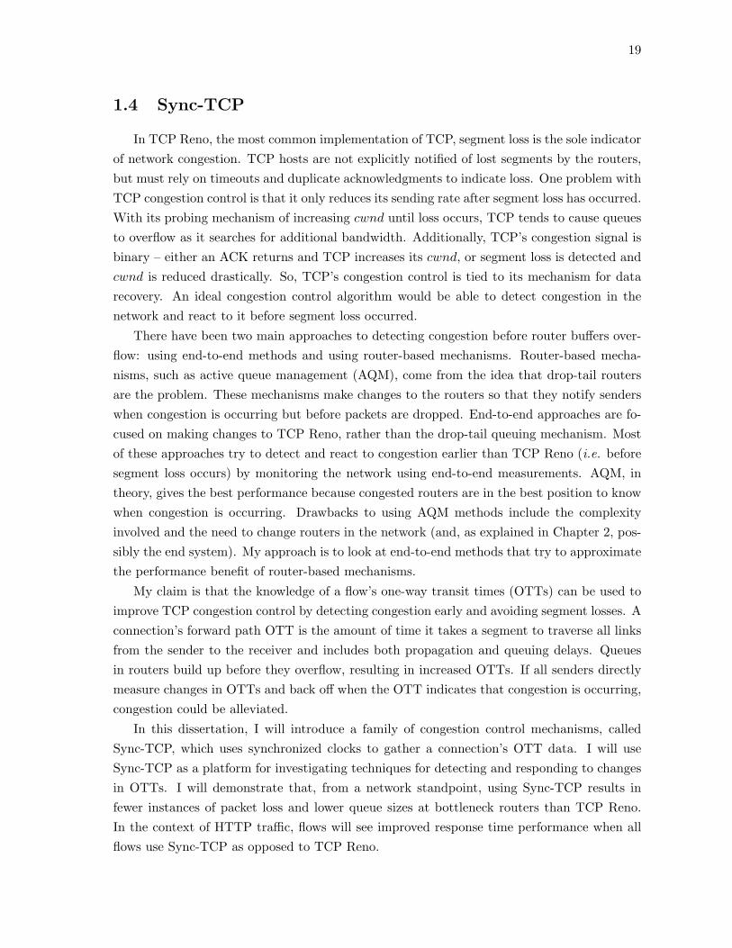
Figure 1.1: Circuit-Switching Example

this section, I will describe a packet-switched network (and also a circuit-switched network),connection-oriented communication (and also connectionless communication), and TCP.

1.1.1 Circuit-Switching vs. Packet-Switching

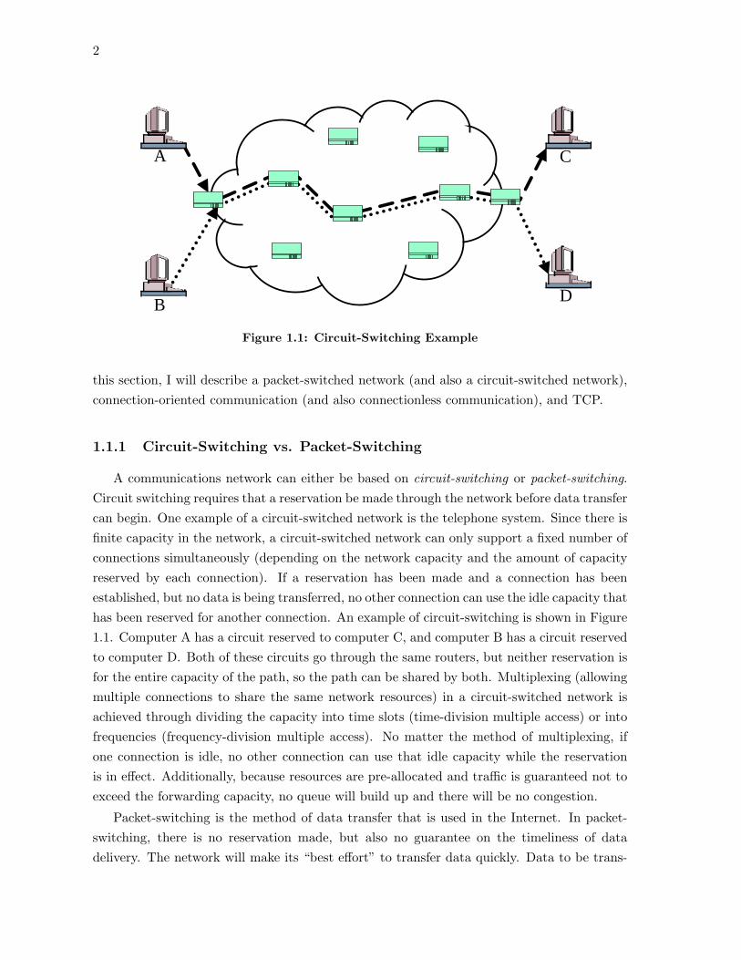
A communications network can either be based on circuit-switching or packet-switching.Circuit switching requires that a reservation be made through the network before data transfercan begin. One example of a circuit-switched network is the telephone system. Since there isfinite capacity in the network, a circuit-switched network can only support a fixed number ofconnections simultaneously (depending on the network capacity and the amount of capacityreserved by each connection). If a reservation has been made and a connection has beenestablished, but no data is being transferred, no other connection can use the idle capacity thathas been reserved for another connection. An example of circuit-switching is shown in Figure1.1. Computer A has a circuit reserved to computer C, and computer B has a circuit reservedto computer D. Both of these circuits go through the same routers, but neither reservation isfor the entire capacity of the path, so the path can be shared by both. Multiplexing (allowingmultiple connections to share the same network resources) in a circuit-switched network isachieved through dividing the capacity into time slots (time-division multiple access) or intofrequencies (frequency-division multiple access). No matter the method of multiplexing, ifone connection is idle, no other connection can use that idle capacity while the reservationis in effect. Additionally, because resources are pre-allocated and traffic is guaranteed not toexceed the forwarding capacity, no queue will build up and there will be no congestion.

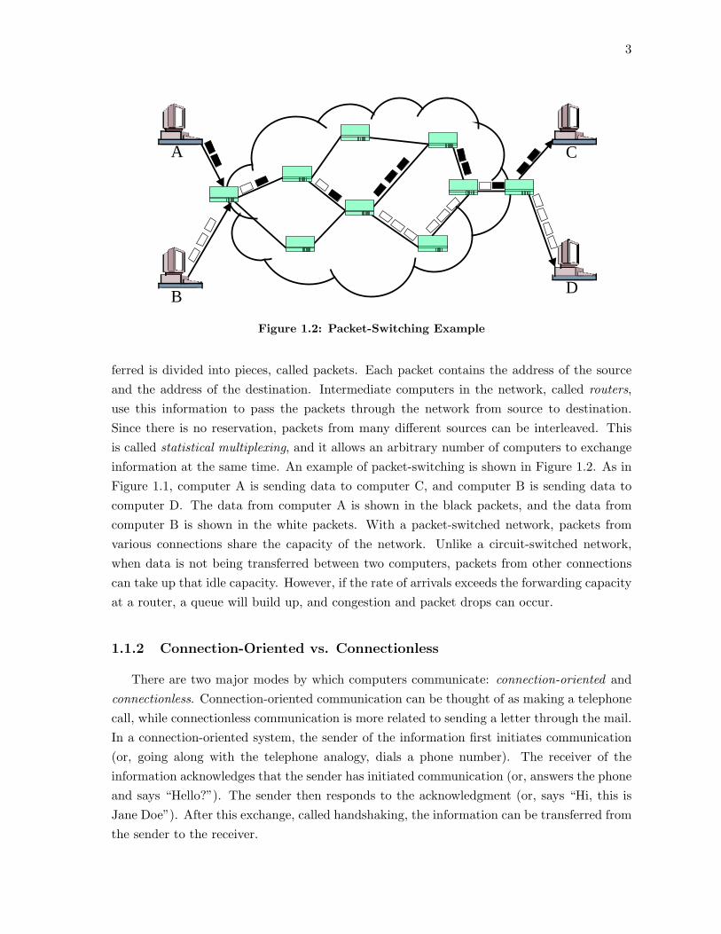
Packet-switching is the method of data transfer that is used in the Internet. In packet-switching, there is no reservation made, but also no guarantee on the timeliness of datadelivery. The network will make its “best effort” to transfer data quickly. Data to be trans-

3

A

B

C

D

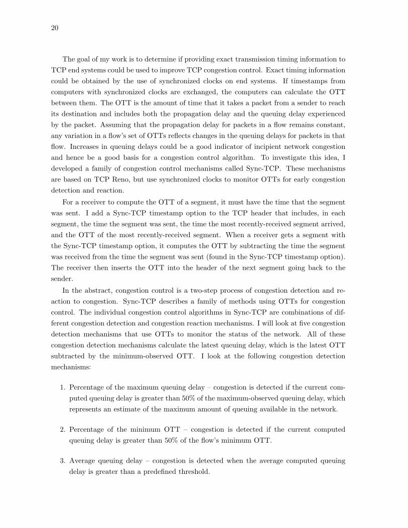
Figure 1.2: Packet-Switching Example

ferred is divided into pieces, called packets. Each packet contains the address of the sourceand the address of the destination. Intermediate computers in the network, called routers,use this information to pass the packets through the network from source to destination.Since there is no reservation, packets from many different sources can be interleaved. Thisis called statistical multiplexing, and it allows an arbitrary number of computers to exchangeinformation at the same time. An example of packet-switching is shown in Figure 1.2. As inFigure 1.1, computer A is sending data to computer C, and computer B is sending data tocomputer D. The data from computer A is shown in the black packets, and the data fromcomputer B is shown in the white packets. With a packet-switched network, packets fromvarious connections share the capacity of the network. Unlike a circuit-switched network,when data is not being transferred between two computers, packets from other connectionscan take up that idle capacity. However, if the rate of arrivals exceeds the forwarding capacityat a router, a queue will build up, and congestion and packet drops can occur.

1.1.2 Connection-Oriented vs. Connectionless

There are two major modes by which computers communicate: connection-oriented andconnectionless. Connection-oriented communication can be thought of as making a telephonecall, while connectionless communication is more related to sending a letter through the mail.In a connection-oriented system, the sender of the information first initiates communication(or, going along with the telephone analogy, dials a phone number). The receiver of theinformation acknowledges that the sender has initiated communication (or, answers the phoneand says “Hello?”). The sender then responds to the acknowledgment (or, says “Hi, this isJane Doe”). After this exchange, called handshaking, the information can be transferred fromthe sender to the receiver.

4

In a connectionless system, there is no handshaking. Information is sent from the senderto the receiver with no acknowledgment, much like the process of writing a letter and puttingit into a mailbox. Like the postal service, in connectionless communication, the sender doesnot know when, or even if, the information was received by the intended party.

The Internet provides a connectionless service, UDP, and a connection-oriented service,TCP. TCP is used for the transfer of many applications, including email, data files, and webpages. I will focus on this connection-oriented service since my dissertation is directly relatedto TCP.

1.1.3 TCP Transport

TCP is the Internet’s connection-oriented transport service. Since the Internet is packet-switched, TCP divides information to be sent into TCP segments, which are then packagedinto packets, containing the addresses of the source and destination. TCP promises reliable,in-order delivery from source to destination. To ensure reliable delivery, all segments areacknowledged by the receiver. Every segment from the sender is sent with a sequence num-ber identifying which bytes the segment contains. Acknowledgments (ACKs) in TCP arecumulative and acknowledge the in-order receipt of all bytes through the sequence numberreturned in the ACK (i.e., the ACK identifies the sequence number of the next in-order bytethe receiver expects to receive from the sender). A TCP sender uses these ACKs to computethe send window, which roughly keeps track of how much data has been sent but not yetacknowledged. To provide in-order delivery, the TCP receiver must buffer any segments thatare received out-of-order until gaps in the sequence number space have been filled.

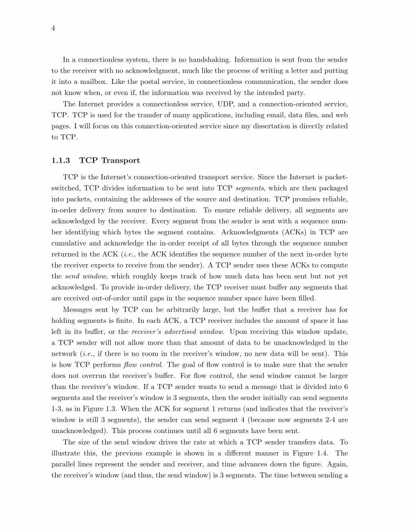
Messages sent by TCP can be arbitrarily large, but the buffer that a receiver has forholding segments is finite. In each ACK, a TCP receiver includes the amount of space it hasleft in its buffer, or the receiver’s advertised window. Upon receiving this window update,a TCP sender will not allow more than that amount of data to be unacknowledged in thenetwork (i.e., if there is no room in the receiver’s window, no new data will be sent). Thisis how TCP performs flow control. The goal of flow control is to make sure that the senderdoes not overrun the receiver’s buffer. For flow control, the send window cannot be largerthan the receiver’s window. If a TCP sender wants to send a message that is divided into 6segments and the receiver’s window is 3 segments, then the sender initially can send segments1-3, as in Figure 1.3. When the ACK for segment 1 returns (and indicates that the receiver’swindow is still 3 segments), the sender can send segment 4 (because now segments 2-4 areunacknowledged). This process continues until all 6 segments have been sent.

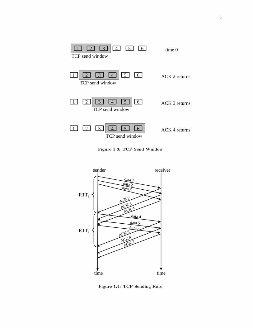
The size of the send window drives the rate at which a TCP sender transfers data. Toillustrate this, the previous example is shown in a different manner in Figure 1.4. Theparallel lines represent the sender and receiver, and time advances down the figure. Again,the receiver’s window (and thus, the send window) is 3 segments. The time between sending a

5

1 2 3 4 5 6 time 0TCP send window

1 2 3 4 5 6 ACK 2 returnsTCP send window

1 2 3 4 5 6 ACK 3 returnsTCP send window

1 2 3 4 5 6 ACK 4 returnsTCP send window

Figure 1.3: TCP Send Window

sender receiver

data 1

time time

data 2data 3

data 4

ACK 3

ACK 4

data 5data 6

ACK 2RTT1

RTT2

ACK 6

ACK 7

ACK 5

Figure 1.4: TCP Sending Rate

6

sender receiver

data 1

time time

data 2data 3

data 4ACK 2

ACK 2

ACK 2

X

data 2

timeout

ACK 5

data 3data 4

Figure 1.5: TCP Drop and Recovery

segment and receiving an ACK for that segment is called the round-trip time (RTT). With aninitial window of 3 segments, TCP will send the first 3 segments out back-to-back. The ACKsfor these segments will also arrive closely-spaced. RTT1 represents the RTT of segment 1,and RTT2 represents the RTT of segment 4 (sent after the ACK for segment 1 was received).The sending rate of this transfer is 3 segments per RTT, since, on average, 3 segments aresent every RTT. More generally, the rate of a TCP sender can be represented in the followingequation:

rate = w/RTT,

where w is the window size.

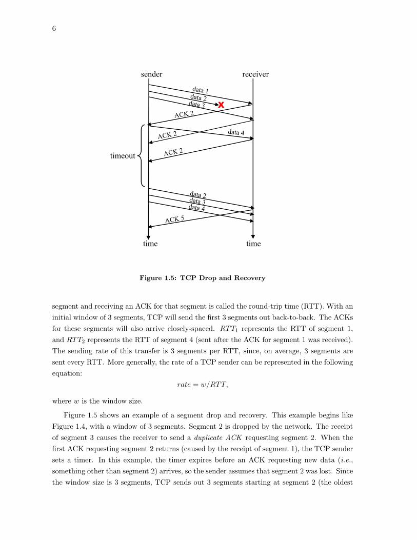
Figure 1.5 shows an example of a segment drop and recovery. This example begins likeFigure 1.4, with a window of 3 segments. Segment 2 is dropped by the network. The receiptof segment 3 causes the receiver to send a duplicate ACK requesting segment 2. When thefirst ACK requesting segment 2 returns (caused by the receipt of segment 1), the TCP sendersets a timer. In this example, the timer expires before an ACK requesting new data (i.e.,something other than segment 2) arrives, so the sender assumes that segment 2 was lost. Sincethe window size is 3 segments, TCP sends out 3 segments starting at segment 2 (the oldest

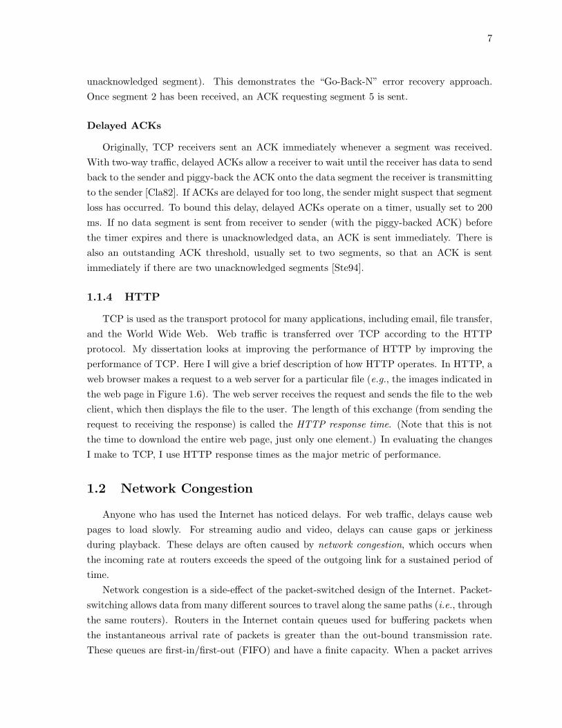
7

unacknowledged segment). This demonstrates the “Go-Back-N” error recovery approach.Once segment 2 has been received, an ACK requesting segment 5 is sent.

Delayed ACKs

Originally, TCP receivers sent an ACK immediately whenever a segment was received.With two-way traffic, delayed ACKs allow a receiver to wait until the receiver has data to sendback to the sender and piggy-back the ACK onto the data segment the receiver is transmittingto the sender [Cla82]. If ACKs are delayed for too long, the sender might suspect that segmentloss has occurred. To bound this delay, delayed ACKs operate on a timer, usually set to 200ms. If no data segment is sent from receiver to sender (with the piggy-backed ACK) beforethe timer expires and there is unacknowledged data, an ACK is sent immediately. There isalso an outstanding ACK threshold, usually set to two segments, so that an ACK is sentimmediately if there are two unacknowledged segments [Ste94].

1.1.4 HTTP

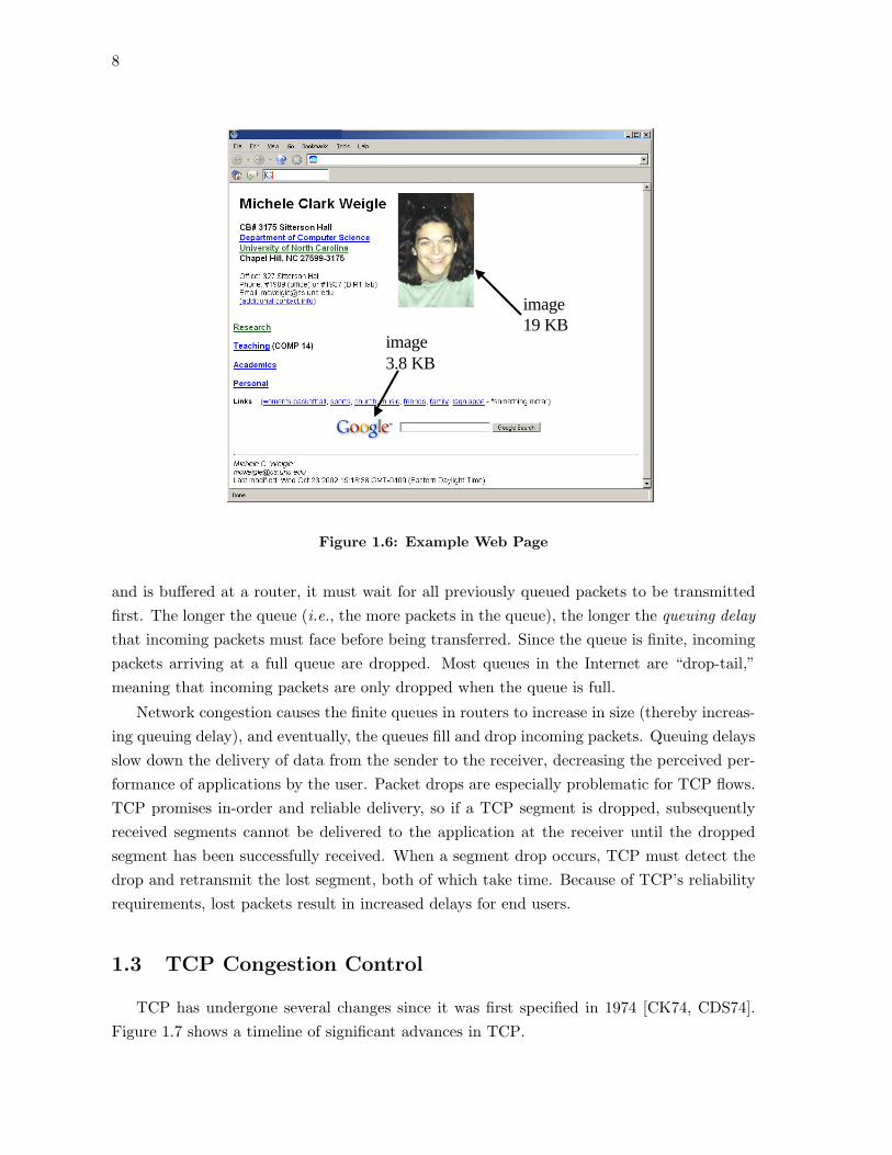
TCP is used as the transport protocol for many applications, including email, file transfer,and the World Wide Web. Web traffic is transferred over TCP according to the HTTPprotocol. My dissertation looks at improving the performance of HTTP by improving theperformance of TCP. Here I will give a brief description of how HTTP operates. In HTTP, aweb browser makes a request to a web server for a particular file (e.g., the images indicated inthe web page in Figure 1.6). The web server receives the request and sends the file to the webclient, which then displays the file to the user. The length of this exchange (from sending therequest to receiving the response) is called the HTTP response time. (Note that this is notthe time to download the entire web page, just only one element.) In evaluating the changesI make to TCP, I use HTTP response times as the major metric of performance.

1.2 Network Congestion

Anyone who has used the Internet has noticed delays. For web traffic, delays cause webpages to load slowly. For streaming audio and video, delays can cause gaps or jerkinessduring playback. These delays are often caused by network congestion, which occurs whenthe incoming rate at routers exceeds the speed of the outgoing link for a sustained period oftime.

Network congestion is a side-effect of the packet-switched design of the Internet. Packet-switching allows data from many different sources to travel along the same paths (i.e., throughthe same routers). Routers in the Internet contain queues used for buffering packets whenthe instantaneous arrival rate of packets is greater than the out-bound transmission rate.These queues are first-in/first-out (FIFO) and have a finite capacity. When a packet arrives

8

image19 KB

image3.8 KB

Figure 1.6: Example Web Page

and is buffered at a router, it must wait for all previously queued packets to be transmittedfirst. The longer the queue (i.e., the more packets in the queue), the longer the queuing delaythat incoming packets must face before being transferred. Since the queue is finite, incomingpackets arriving at a full queue are dropped. Most queues in the Internet are “drop-tail,”meaning that incoming packets are only dropped when the queue is full.

Network congestion causes the finite queues in routers to increase in size (thereby increas-ing queuing delay), and eventually, the queues fill and drop incoming packets. Queuing delaysslow down the delivery of data from the sender to the receiver, decreasing the perceived per-formance of applications by the user. Packet drops are especially problematic for TCP flows.TCP promises in-order and reliable delivery, so if a TCP segment is dropped, subsequentlyreceived segments cannot be delivered to the application at the receiver until the droppedsegment has been successfully received. When a segment drop occurs, TCP must detect thedrop and retransmit the lost segment, both of which take time. Because of TCP’s reliabilityrequirements, lost packets result in increased delays for end users.

1.3 TCP Congestion Control

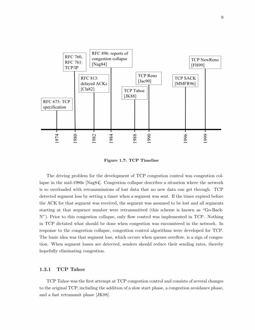
TCP has undergone several changes since it was first specified in 1974 [CK74, CDS74].Figure 1.7 shows a timeline of significant advances in TCP.

9

1984

RFC 896: reports ofcongestion collapse[Nag84]

1988

TCP Tahoe[JK88]

1990

TCP Reno[Jac90]

1999

TCP NewReno[FH99]

1996

TCP SACK[MMFR96]

1974

RFC 675: TCPspecification

1982

RFC 813:delayed ACKs[Cla82]

1980

RFC 760,RFC 761:TCP/IP

Figure 1.7: TCP Timeline

The driving problem for the development of TCP congestion control was congestion col-lapse in the mid-1980s [Nag84]. Congestion collapse describes a situation where the networkis so overloaded with retransmissions of lost data that no new data can get through. TCPdetected segment loss by setting a timer when a segment was sent. If the timer expired beforethe ACK for that segment was received, the segment was assumed to be lost and all segmentsstarting at that sequence number were retransmitted (this scheme is known as “Go-Back-N”). Prior to this congestion collapse, only flow control was implemented in TCP. Nothingin TCP dictated what should be done when congestion was encountered in the network. Inresponse to the congestion collapse, congestion control algorithms were developed for TCP.The basic idea was that segment loss, which occurs when queues overflow, is a sign of conges-tion. When segment losses are detected, senders should reduce their sending rates, therebyhopefully eliminating congestion.

1.3.1 TCP Tahoe

TCP Tahoe was the first attempt at TCP congestion control and consists of several changesto the original TCP, including the addition of a slow start phase, a congestion avoidance phase,and a fast retransmit phase [JK88].

10

Slow Start

TCP follows the idea of conservation of packets. A new segment is not sent into thenetwork until a segment has left the network (i.e., an ACK has returned). Before TCP Tahoewas introduced, TCP obeyed conservation of packets except upon startup. At startup, thereare no outstanding segments to be acknowledged to release new segments, so TCP senderssent out a full window’s worth of segments at once. The TCP senders, though, have noindication of how much data the network can handle at once, so often, these bursts led topackets being dropped at routers.

At startup (and after a packet loss), instead of sending segments as fast as possible, slowstart restricts the rate of segments entering the network to twice the rate that ACKs returnfrom the receiver. TCP Tahoe introduced the congestion window, cwnd, initially set to onesegment. The send window is set to the minimum of cwnd and the receiver’s advertisedwindow. For every ACK received, cwnd is incremented by one segment. The size of the sendwindow controls the sending rate of a TCP sender (rate = w/RTT ). To increase its sendingrate, a TCP sender would increase the value of its send window by increasing cwnd, allowingadditional data to be transferred into the network before the first segment in the congestionwindow has been acknowledged. The congestion window can only be increased when ACKsreturn from the receiver, since ACKs indicate that data has been successfully delivered. ATCP sender will keep increasing cwnd until it detects that network congestion is occurring.

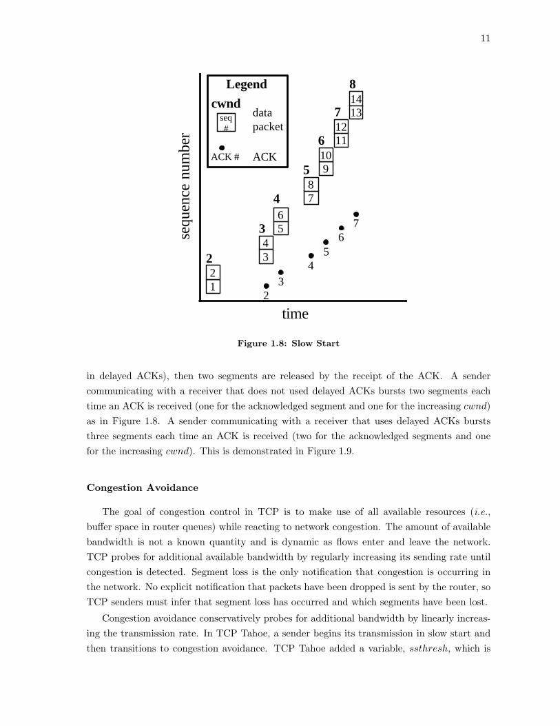
Figure 1.8 shows an example of the operation of slow start. The x-axis is time andthe y-axis is sequence number. The boxes represent the transmission of a segment and arelabeled with their corresponding sequence numbers. In order keep the example simple, I amassuming 1-byte segments. The numbers above the boxes indicate the value of cwnd whenthose segments were sent. Dots represent the arrival of an ACK and are centered along they-axis of the highest sequence number they acknowledge. The ACKs are also centered alongthe x-axis with the segments that are released by the arrival of the ACK. The numbers belowthe ACKs represent the sequence number carried in the ACK (i.e., the sequence number ofthe next segment expected by the receiver), referred to as the ACK number. For example,the first dot represents the acknowledgment of the receipt of segment 1 and that the receiverexpects to next receive segment 2. So, the dot is positioned on the y-axis centered on segment1 with a 2 below the dot, indicating that the ACK carries the ACK number of 2. In Figure1.8, the initial value of cwnd is 2, so segments 1 and 2 are sent at time 0. When the ACK forsegment 1 is received, cwnd is incremented to 3, and segments 3 and 4 are sent – segment 3 isreleased because segment 1 has been acknowledged and is no longer outstanding and segment4 is sent to fill the congestion window. Thus, during slow start, for each ACK that is received,two new segments are sent.

During slow start, the sender’s congestion window grows by one segment each time anACK for new data is received. If an ACK acknowledges the receipt of two segments (as

11

2

time

sequ

ence

num

ber

34

56

78

12

2

3

4

9106 11

127 13

148

5

Legend

ACK #

seq#

cwnddatapacket

ACK

34

56

7

Figure 1.8: Slow Start

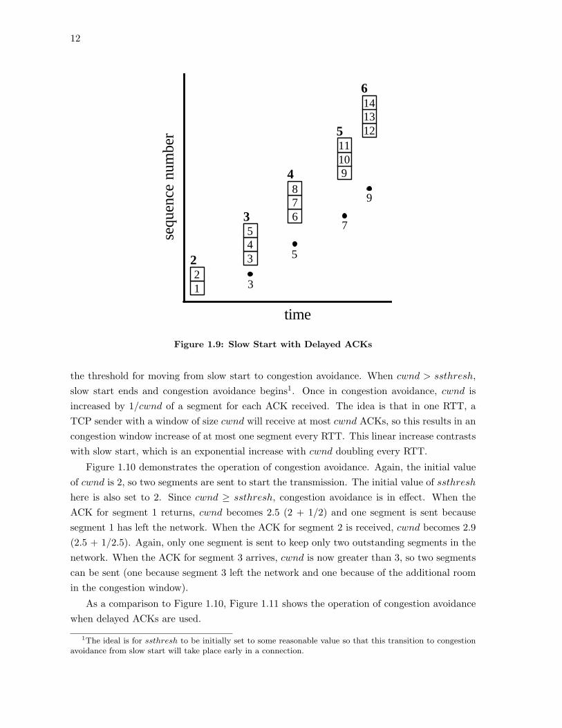
in delayed ACKs), then two segments are released by the receipt of the ACK. A sendercommunicating with a receiver that does not used delayed ACKs bursts two segments eachtime an ACK is received (one for the acknowledged segment and one for the increasing cwnd)as in Figure 1.8. A sender communicating with a receiver that uses delayed ACKs burststhree segments each time an ACK is received (two for the acknowledged segments and onefor the increasing cwnd). This is demonstrated in Figure 1.9.

Congestion Avoidance

The goal of congestion control in TCP is to make use of all available resources (i.e.,buffer space in router queues) while reacting to network congestion. The amount of availablebandwidth is not a known quantity and is dynamic as flows enter and leave the network.TCP probes for additional available bandwidth by regularly increasing its sending rate untilcongestion is detected. Segment loss is the only notification that congestion is occurring inthe network. No explicit notification that packets have been dropped is sent by the router, soTCP senders must infer that segment loss has occurred and which segments have been lost.

Congestion avoidance conservatively probes for additional bandwidth by linearly increas-ing the transmission rate. In TCP Tahoe, a sender begins its transmission in slow start andthen transitions to congestion avoidance. TCP Tahoe added a variable, ssthresh, which is

12

time

sequ

ence

num

ber

345

678

12

2

3

4 910

511

1213146

3

5

7

9

Figure 1.9: Slow Start with Delayed ACKs

the threshold for moving from slow start to congestion avoidance. When cwnd > ssthresh,slow start ends and congestion avoidance begins1. Once in congestion avoidance, cwnd isincreased by 1/cwnd of a segment for each ACK received. The idea is that in one RTT, aTCP sender with a window of size cwnd will receive at most cwnd ACKs, so this results in ancongestion window increase of at most one segment every RTT. This linear increase contrastswith slow start, which is an exponential increase with cwnd doubling every RTT.

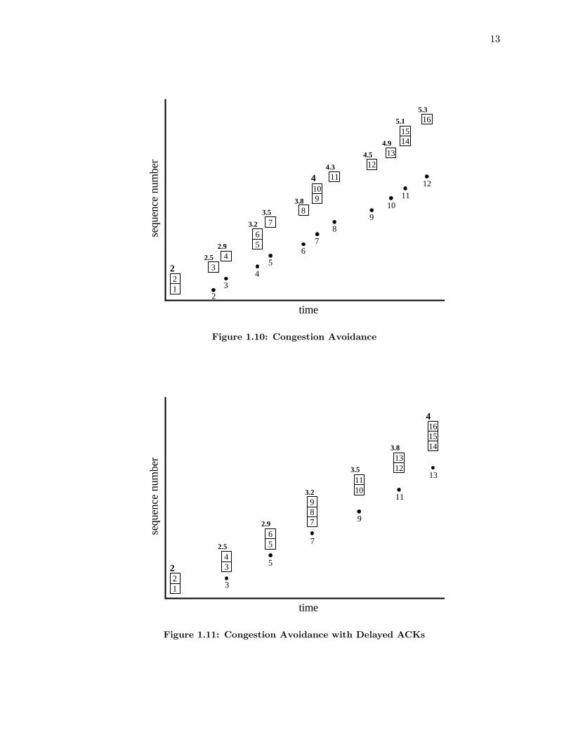
Figure 1.10 demonstrates the operation of congestion avoidance. Again, the initial valueof cwnd is 2, so two segments are sent to start the transmission. The initial value of ssthreshhere is also set to 2. Since cwnd ≥ ssthresh, congestion avoidance is in effect. When theACK for segment 1 returns, cwnd becomes 2.5 (2 + 1/2) and one segment is sent becausesegment 1 has left the network. When the ACK for segment 2 is received, cwnd becomes 2.9(2.5 + 1/2.5). Again, only one segment is sent to keep only two outstanding segments in thenetwork. When the ACK for segment 3 arrives, cwnd is now greater than 3, so two segmentscan be sent (one because segment 3 left the network and one because of the additional roomin the congestion window).

As a comparison to Figure 1.10, Figure 1.11 shows the operation of congestion avoidancewhen delayed ACKs are used.

1The ideal is for ssthresh to be initially set to some reasonable value so that this transition to congestionavoidance from slow start will take place early in a connection.

13

time

sequ

ence

num

ber

34

56

78

12

2

2.9

9104 11

2.5

3.2

3.5

3.8

4.3 124.5 13

4.9 1415

5.1 165.3

23

45

67

89

1011

12

Figure 1.10: Congestion Avoidance

time

sequ

ence

num

ber

34

56

78

12

2

2.5

91011

2.9

3.2

3.5 1213

3.8 141516

4

3

5

7

9

11

13

Figure 1.11: Congestion Avoidance with Delayed ACKs

14

Fast Retransmit

TCP uses a timer to detect when segments can be assumed to be lost and should beretransmitted. This retransmission timeout (RTO) timer is set every time a data segment issent (if the timer has not already been set). Whenever an ACK for new data is received, theRTO timer is reset. If the RTO timer expires before the next ACK for new data arrives, theoldest unacknowledged segment is assumed to be lost and will be retransmitted. The RTOtimer is set to 3-4 times the RTT so that unnecessary retransmissions are not generated bysegments being delayed in the network. With the addition of congestion avoidance in TCPTahoe, when the RTO timer expires (i.e., when a segment is assumed to be lost), 1/2 cwndis saved in ssthresh2 and cwnd is set to 1 segment. At this point, cwnd < ssthresh, soa timeout marks a return to slow start. As slow start progresses, if no additional segmentloss occurs, once cwnd reaches ssthresh (which is 1/2 of cwnd when segment loss was lastdetected), congestion avoidance is entered.

TCP Tahoe also added a faster way to detect segment loss, called fast retransmit. BeforeTCP Tahoe, the only way to detect segment loss was through the expiration of the RTO timer.TCP Tahoe added the ability to infer segment loss through the receipt of three duplicateACKs. Whenever a receiver sees an out-of-order segment (e.g., a gap in sequence numbers),it sends an ACK for the last in-order segment it received (which would be a duplicate of theprevious ACK sent). The sender uses the receipt of three duplicates of the same ACK to inferthat there was segment loss rather just segment re-ordering.

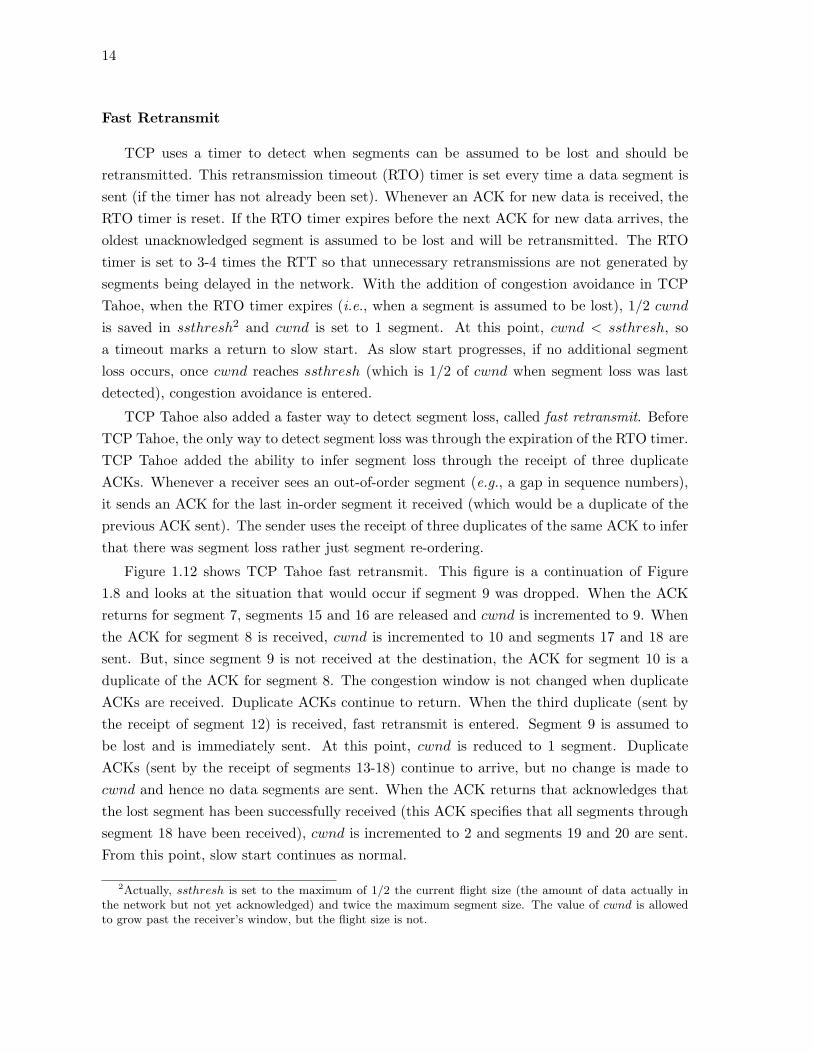
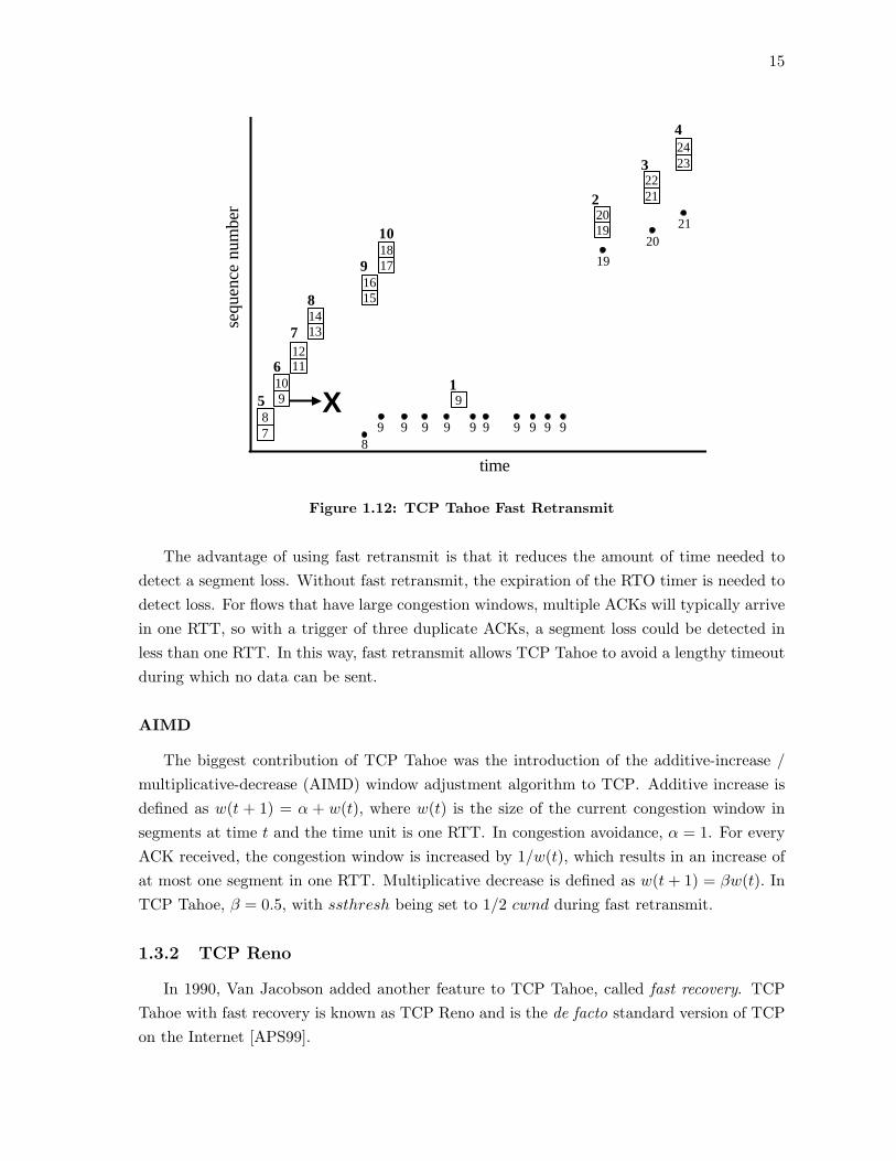
Figure 1.12 shows TCP Tahoe fast retransmit. This figure is a continuation of Figure1.8 and looks at the situation that would occur if segment 9 was dropped. When the ACKreturns for segment 7, segments 15 and 16 are released and cwnd is incremented to 9. Whenthe ACK for segment 8 is received, cwnd is incremented to 10 and segments 17 and 18 aresent. But, since segment 9 is not received at the destination, the ACK for segment 10 is aduplicate of the ACK for segment 8. The congestion window is not changed when duplicateACKs are received. Duplicate ACKs continue to return. When the third duplicate (sent bythe receipt of segment 12) is received, fast retransmit is entered. Segment 9 is assumed tobe lost and is immediately sent. At this point, cwnd is reduced to 1 segment. DuplicateACKs (sent by the receipt of segments 13-18) continue to arrive, but no change is made tocwnd and hence no data segments are sent. When the ACK returns that acknowledges thatthe lost segment has been successfully received (this ACK specifies that all segments throughsegment 18 have been received), cwnd is incremented to 2 and segments 19 and 20 are sent.From this point, slow start continues as normal.

2Actually, ssthresh is set to the maximum of 1/2 the current flight size (the amount of data actually inthe network but not yet acknowledged) and twice the maximum segment size. The value of cwnd is allowedto grow past the receiver’s window, but the flight size is not.

15

time

sequ

ence

num

ber

9 X 910

1112

1314

78

5

6

7

8 15169 17

1810

1

1920

2 2122

3 23244

89 9 9 9 9 99 9 9 9

1920

21

Figure 1.12: TCP Tahoe Fast Retransmit

The advantage of using fast retransmit is that it reduces the amount of time needed todetect a segment loss. Without fast retransmit, the expiration of the RTO timer is needed todetect loss. For flows that have large congestion windows, multiple ACKs will typically arrivein one RTT, so with a trigger of three duplicate ACKs, a segment loss could be detected inless than one RTT. In this way, fast retransmit allows TCP Tahoe to avoid a lengthy timeoutduring which no data can be sent.

AIMD

The biggest contribution of TCP Tahoe was the introduction of the additive-increase /multiplicative-decrease (AIMD) window adjustment algorithm to TCP. Additive increase isdefined as w(t + 1) = α + w(t), where w(t) is the size of the current congestion window insegments at time t and the time unit is one RTT. In congestion avoidance, α = 1. For everyACK received, the congestion window is increased by 1/w(t), which results in an increase ofat most one segment in one RTT. Multiplicative decrease is defined as w(t+ 1) = βw(t). InTCP Tahoe, β = 0.5, with ssthresh being set to 1/2 cwnd during fast retransmit.

1.3.2 TCP Reno

In 1990, Van Jacobson added another feature to TCP Tahoe, called fast recovery. TCPTahoe with fast recovery is known as TCP Reno and is the de facto standard version of TCPon the Internet [APS99].

16

time

sequ

ence

num

ber

9 X 910

1112

1314

78

5

6

7

8 15169 17

1810

8

1911 20

12 2113 22

14 235 24

5.2 255.3 26

5.5

89 9 9 99 9 99 9 9

19

2021

22

Figure 1.13: TCP Reno Fast Retransmit and Fast Recovery

Fast Recovery

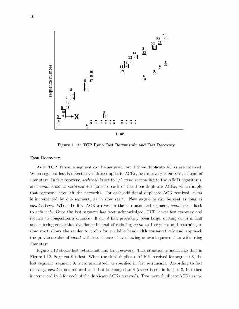
As in TCP Tahoe, a segment can be assumed lost if three duplicate ACKs are received.When segment loss is detected via three duplicate ACKs, fast recovery is entered, instead ofslow start. In fast recovery, ssthresh is set to 1/2 cwnd (according to the AIMD algorithm),and cwnd is set to ssthresh + 3 (one for each of the three duplicate ACKs, which implythat segments have left the network). For each additional duplicate ACK received, cwndis incremented by one segment, as in slow start. New segments can be sent as long ascwnd allows. When the first ACK arrives for the retransmitted segment, cwnd is set backto ssthresh. Once the lost segment has been acknowledged, TCP leaves fast recovery andreturns to congestion avoidance. If cwnd had previously been large, cutting cwnd in halfand entering congestion avoidance instead of reducing cwnd to 1 segment and returning toslow start allows the sender to probe for available bandwidth conservatively and approachthe previous value of cwnd with less chance of overflowing network queues than with usingslow start.

Figure 1.13 shows fast retransmit and fast recovery. This situation is much like that inFigure 1.12. Segment 9 is lost. When the third duplicate ACK is received for segment 8, thelost segment, segment 9, is retransmitted, as specified in fast retransmit. According to fastrecovery, cwnd is not reduced to 1, but is changed to 8 (cwnd is cut in half to 5, but thenincremented by 3 for each of the duplicate ACKs received). Two more duplicate ACKs arrive

17

after the retransmission and, for each of these, cwnd is incremented. So, cwnd is 10, but noadditional segments can be sent because as far as the TCP sender knows, 10 segments areoutstanding (segments 9-18). When the ACK sent by the receipt of segment 15 is received,cwnd is again incremented. Since cwnd is now 11, there is room for one more segment to besent, and so, segment 19 is released. This continues until the retransmission of segment 9 isacknowledged. When this occurs, cwnd is returned to 5 (one-half of the congestion windowwhen loss was detected) and congestion avoidance is entered and progresses as normal.

As seen in the example above, fast recovery also provides an additional transition fromslow start to congestion avoidance. If a sender is in slow start and detects segment lossthrough three duplicate ACKs, after the loss has been recovered, congestion avoidance isentered. As in TCP Tahoe, congestion avoidance is also entered whenever cwnd > ssthresh.In many cases, though, the initial value of ssthresh is set to a very large value (e.g., 1 MB inFreeBSD 5.0), so segment loss is often the only trigger to enter congestion avoidance [Hoe96].

TCP Reno is limited to recovering from only one segment loss during a single fast re-transmit and fast recovery phase. Additional segment losses in the same window may requirethat the RTO timer expire before the segments can be retransmitted. The exception is whencwnd is greater than 10 segments upon entering fast recovery, allowing two segment lossesto be recovered without the sender experiencing a timeout. During fast recovery, one of thenew segments to be sent (after the retransmission) could be lost and detected with threeduplicate ACKs after the first fast recovery has finished (with the receipt of the ACK forthe retransmitted packet). In this case, TCP Reno could recover from two segment lossesby entering fast recovery twice in succession. This causes cwnd to effectively be reduced by75% in two RTTs. This situation is demonstrated by Fall and Floyd when two segments aredropped [FF96].

1.3.3 Selective Acknowledgments

A recent addition to the standard TCP implementation is the selective acknowledgmentoption (SACK) [MMFR96]. SACK is used in loss recovery and helps the sender determinewhich segments have been dropped in the case of multiple losses in a window. The SACKoption contains up to four (or three, if the RFC 1323 timestamp option is used) SACK blocks,which specify contiguous blocks of the most recently received data. Each SACK block consistsof two sequence numbers which delimit the range of data the receiver holds. A receiver can addthe SACK option to ACKs it sends back to a SACK-enabled sender. Using the informationin the SACK blocks, the sender can infer which segments have been lost (up to three non-contiguous blocks of lost segments). The SACK option is sent only on ACKs that occur afterout-of-order segments have been received. Allowing up to three SACK blocks per SACKoption ensures that each SACK block is transmitted in at least three ACKs, providing someamount of robustness in the face of ACK loss.

18

The SACK RFC specifies only the SACK option and not how a sender should use theinformation given in the SACK option. Blanton et al. present a method for using the SACKoption for efficient data recovery [MMFR96]. This method was based on an implementationof SACK by Fall and Floyd [FF96]. The SACK recovery algorithm only operates once fastrecovery has been entered via the receipt of three duplicate ACKs. The use of SACK allowsTCP to decouple the issues of when to retransmit a segment from which segment to send.To do this, SACK adds two variables to TCP: scoreboard (which segments to send) and pipe(when to send segments).

The scoreboard records which segments the sender infers to be lost based on informationfrom SACKs. The segments in the scoreboard all have sequence numbers past the currentvalue of the highest cumulative ACK. During fast recovery, pipe is the estimate of the amountof unacknowledged data “in the pipe.” Each time a segment is sent, pipe is incremented.The value of pipe is decremented whenever a duplicate ACK arrives with a SACK blockindicating that new data was received. When cwnd− pipe ≥ 1, the sender can either send aretransmission or transmit new data. When the sender is allowed to send data, it first looksat scoreboard and sends any segments needed to fill gaps at the receiver. If there are no suchsegments, then the sender can transmit new data. The sender leaves fast recovery when all ofthe data that was unacknowledged at the beginning of fast recovery has been acknowledged.

1.3.4 TCP NewReno

During fast recovery, TCP Reno can only recover from one segment loss without sufferinga timeout3. As long as duplicate ACKs are returning, the sender can send new segments intothe network, but fast recovery is not over until an ACK for the lost segment is received. Onlyone retransmission is sent during each fast recovery period, though multiple retransmissionscan be triggered by the expiration of the RTO timer.

TCP NewReno is a change to non-SACK-enabled TCP Reno where the sender does notleave fast recovery after a partial ACK is received [Hoe95, FH99]. A partial ACK acknowledgessome, but not all, of the data sent before the segment loss was detected. With the receipt ofa partial ACK, the sender can infer that the next segment the receiver expects has also beenlost. TCP NewReno allows the sender to retransmit more than one segment during a singlefast recovery, but only one lost segment may be retransmitted each RTT.

One recent study has reported that TCP NewReno is the most popular TCP version fora sample of Internet web servers [PF01].

3Except for in the situation described in section 1.3.2.

19

1.4 Sync-TCP

In TCP Reno, the most common implementation of TCP, segment loss is the sole indicatorof network congestion. TCP hosts are not explicitly notified of lost segments by the routers,but must rely on timeouts and duplicate acknowledgments to indicate loss. One problem withTCP congestion control is that it only reduces its sending rate after segment loss has occurred.With its probing mechanism of increasing cwnd until loss occurs, TCP tends to cause queuesto overflow as it searches for additional bandwidth. Additionally, TCP’s congestion signal isbinary – either an ACK returns and TCP increases its cwnd, or segment loss is detected andcwnd is reduced drastically. So, TCP’s congestion control is tied to its mechanism for datarecovery. An ideal congestion control algorithm would be able to detect congestion in thenetwork and react to it before segment loss occurred.

There have been two main approaches to detecting congestion before router buffers over-flow: using end-to-end methods and using router-based mechanisms. Router-based mecha-nisms, such as active queue management (AQM), come from the idea that drop-tail routersare the problem. These mechanisms make changes to the routers so that they notify senderswhen congestion is occurring but before packets are dropped. End-to-end approaches are fo-cused on making changes to TCP Reno, rather than the drop-tail queuing mechanism. Mostof these approaches try to detect and react to congestion earlier than TCP Reno (i.e. beforesegment loss occurs) by monitoring the network using end-to-end measurements. AQM, intheory, gives the best performance because congested routers are in the best position to knowwhen congestion is occurring. Drawbacks to using AQM methods include the complexityinvolved and the need to change routers in the network (and, as explained in Chapter 2, pos-sibly the end system). My approach is to look at end-to-end methods that try to approximatethe performance benefit of router-based mechanisms.

My claim is that the knowledge of a flow’s one-way transit times (OTTs) can be used toimprove TCP congestion control by detecting congestion early and avoiding segment losses. Aconnection’s forward path OTT is the amount of time it takes a segment to traverse all linksfrom the sender to the receiver and includes both propagation and queuing delays. Queuesin routers build up before they overflow, resulting in increased OTTs. If all senders directlymeasure changes in OTTs and back off when the OTT indicates that congestion is occurring,congestion could be alleviated.

In this dissertation, I will introduce a family of congestion control mechanisms, calledSync-TCP, which uses synchronized clocks to gather a connection’s OTT data. I will useSync-TCP as a platform for investigating techniques for detecting and responding to changesin OTTs. I will demonstrate that, from a network standpoint, using Sync-TCP results infewer instances of packet loss and lower queue sizes at bottleneck routers than TCP Reno.In the context of HTTP traffic, flows will see improved response time performance when allflows use Sync-TCP as opposed to TCP Reno.

20

The goal of my work is to determine if providing exact transmission timing information toTCP end systems could be used to improve TCP congestion control. Exact timing informationcould be obtained by the use of synchronized clocks on end systems. If timestamps fromcomputers with synchronized clocks are exchanged, the computers can calculate the OTTbetween them. The OTT is the amount of time that it takes a packet from a sender to reachits destination and includes both the propagation delay and the queuing delay experiencedby the packet. Assuming that the propagation delay for packets in a flow remains constant,any variation in a flow’s set of OTTs reflects changes in the queuing delays for packets in thatflow. Increases in queuing delays could be a good indicator of incipient network congestionand hence be a good basis for a congestion control algorithm. To investigate this idea, Ideveloped a family of congestion control mechanisms called Sync-TCP. These mechanismsare based on TCP Reno, but use synchronized clocks to monitor OTTs for early congestiondetection and reaction.

For a receiver to compute the OTT of a segment, it must have the time that the segmentwas sent. I add a Sync-TCP timestamp option to the TCP header that includes, in eachsegment, the time the segment was sent, the time the most recently-received segment arrived,and the OTT of the most recently-received segment. When a receiver gets a segment withthe Sync-TCP timestamp option, it computes the OTT by subtracting the time the segmentwas received from the time the segment was sent (found in the Sync-TCP timestamp option).The receiver then inserts the OTT into the header of the next segment going back to thesender.

In the abstract, congestion control is a two-step process of congestion detection and re-action to congestion. Sync-TCP describes a family of methods using OTTs for congestioncontrol. The individual congestion control algorithms in Sync-TCP are combinations of dif-ferent congestion detection and congestion reaction mechanisms. I will look at five congestiondetection mechanisms that use OTTs to monitor the status of the network. All of thesecongestion detection mechanisms calculate the latest queuing delay, which is the latest OTTsubtracted by the minimum-observed OTT. I look at the following congestion detectionmechanisms:

1. Percentage of the maximum queuing delay – congestion is detected if the current com-puted queuing delay is greater than 50% of the maximum-observed queuing delay, whichrepresents an estimate of the maximum amount of queuing available in the network.

2. Percentage of the minimum OTT – congestion is detected if the current computedqueuing delay is greater than 50% of the flow’s minimum OTT.

3. Average queuing delay – congestion is detected when the average computed queuingdelay is greater than a predefined threshold.

21

Trend Average Queuing DelayDirection (as a % of the maximum) Adjustment to cwnd

increasing 75-100% decrease cwnd 50%increasing 50-75% decrease cwnd 25%increasing 25-50% decrease cwnd 10%increasing 0-25% increase cwnd 1 segment per RTTdecreasing 75-100% no change to cwnddecreasing 50-75% increase cwnd 10% per RTTdecreasing 25-50% increase cwnd 25% per RTTdecreasing 0-25% increase cwnd 50% per RTT

Table 1.1: Adjustments to the Congestion Window Based on the Signal from the Con-gestion Detection Mechanism

4. Trend analysis of queuing delays – congestion is detected when the trend of nine queuingdelay samples is increasing.

5. Trend analysis of average queuing delay – provides a congestion signal that uses thedirection of the trend of the average computed queuing delay and the value of theaverage computed queuing delay as a percentage of the maximum-observed queuingdelay.

I will show that trend analysis of the average queuing delay (mechanism 5), which is a com-bination of the best parts of mechanisms 1, 3, and 4, offers the best congestion detection.

I look at two congestion reaction mechanisms. The first method is the same as TCPReno’s reaction to the receipt of three duplicate ACKs, where the sender reduces cwnd by50%. This mechanism can operate with any congestion detection mechanism that providesa binary signal of congestion. The second method is based on using the trend analysis ofthe average computed queuing delay as the congestion detection mechanism. Table 1.1 liststhe adjustments that this mechanism makes to cwnd based on the result of the congestiondetection.

1.5 Thesis Statement

My thesis for this work is as follows: Precise knowledge of one-way transit times canbe used to improve the performance of TCP congestion control. Performance is measuredin terms of network-level metrics, including packet loss and average queue sizes at con-gested links, and in terms of application-level metrics, including HTTP response times andthroughput per HTTP response. I will show that Sync-TCP provides lower packet loss, lowerqueue sizes, lower HTTP response times, and higher throughput per HTTP response thanTCP Reno. Additionally, I will show that Sync-TCP offers performance comparable to thatachieved by using router-based congestion control mechanisms.

22

10 Mbps

HTTPclients

HTTPservers

HTTPclients

HTTPservers

Router Router

Figure 1.14: Network Topology

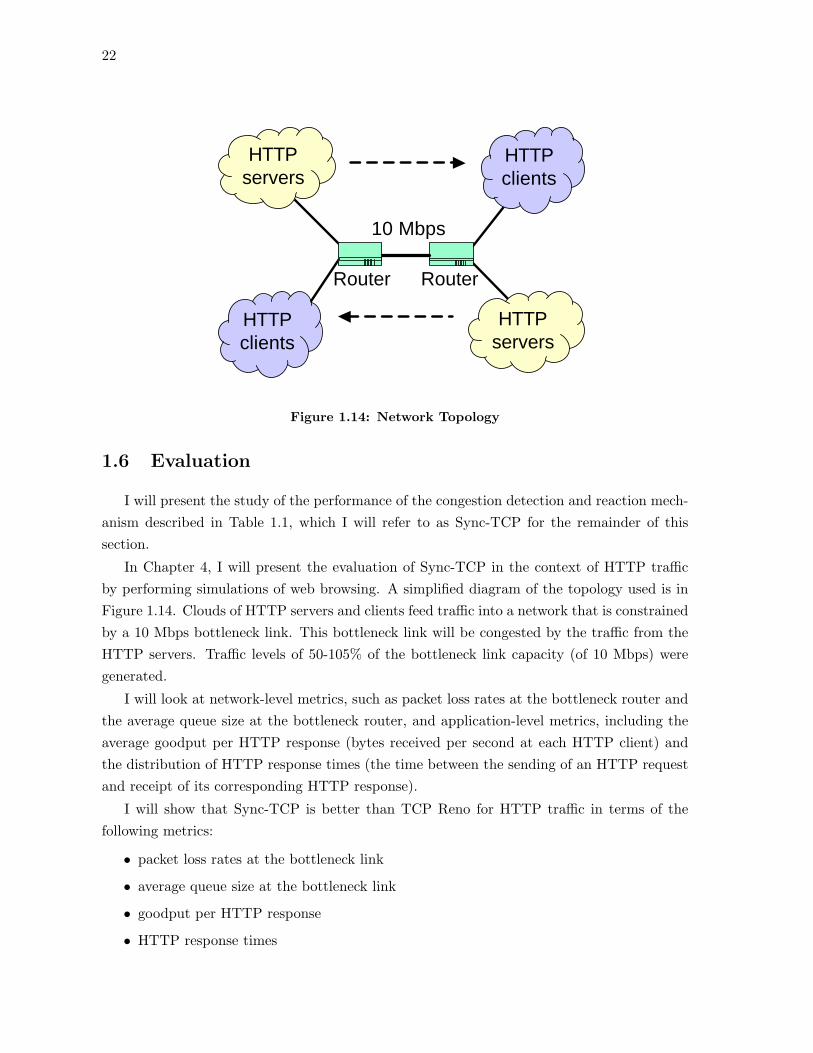
1.6 Evaluation

I will present the study of the performance of the congestion detection and reaction mech-anism described in Table 1.1, which I will refer to as Sync-TCP for the remainder of thissection.

In Chapter 4, I will present the evaluation of Sync-TCP in the context of HTTP trafficby performing simulations of web browsing. A simplified diagram of the topology used is inFigure 1.14. Clouds of HTTP servers and clients feed traffic into a network that is constrainedby a 10 Mbps bottleneck link. This bottleneck link will be congested by the traffic from theHTTP servers. Traffic levels of 50-105% of the bottleneck link capacity (of 10 Mbps) weregenerated.

I will look at network-level metrics, such as packet loss rates at the bottleneck router andthe average queue size at the bottleneck router, and application-level metrics, including theaverage goodput per HTTP response (bytes received per second at each HTTP client) andthe distribution of HTTP response times (the time between the sending of an HTTP requestand receipt of its corresponding HTTP response).

I will show that Sync-TCP is better than TCP Reno for HTTP traffic in terms of thefollowing metrics:

• packet loss rates at the bottleneck link

• average queue size at the bottleneck link

• goodput per HTTP response

• HTTP response times

23

In particular, at load levels of 50% and 60% of the capacity of the bottleneck link, I willshow that using Sync-TCP for all HTTP flows results in 0 drops at the bottleneck link. Incomparison, TCP Reno had over 3500 and 8000 drops, respectively. At all load levels, Sync-TCP provides less packet loss and lower queue sizes, which in turn, resulted in lower HTTPresponse times. If all flows use Sync-TCP to react to increases in queuing delay, congestioncould be alleviated quickly. This would result in overall shorter queues, faster response forinteractive applications, and a more efficient use of network resources.

By showing that Sync-TCP can provide better network performance, I will show thatsynchronized clocks can be used to improve TCP congestion control. In this dissertation, Imake the following contributions:

• a method for measuring a flow’s OTT and returning this exact timing information tothe sender

• a comparison of several methods for using OTTs to detect congestion

• a family of end-to-end congestion control mechanisms, Sync-TCP, based on using OTTsfor congestion detection

• a study of standards-track4 TCP congestion control and error recovery mechanisms inthe context of HTTP traffic, used as a basis for comparison to Sync-TCP

In the remainder of this dissertation, I will first discuss related work in Chapter 2, includingprevious approaches to the congestion control problem. Then, in Chapter 3, I will discussthe various Sync-TCP congestion detection and reaction mechanisms. Chapter 4, presentsresults from a comparison of the best version of Sync-TCP to the best standards-track TCPprotocol in the context of HTTP traffic. A summary of this work and ideas for future workare given in Chapter 5. Appendix A covers the experimental methodology, including detailsof the network configuration, HTTP traffic model, and components I added to the ns networksimulator for running the experiments. Finally, Appendix B describes experiments performedto choose the best standards-track TCP protocol for HTTP traffic.

4By standards-track congestion control, I mean TCP Reno and Adaptive RED, a form of router-basedcongestion control. By standards-track error recovery, I mean TCP Reno and TCP SACK. TCP Reno is anIETF standard, TCP SACK is on the IETF standards track, and Adaptive RED, a modification to the IETFstandard RED, is widely encouraged to be used in Internet routers.