1

CHAPTER 1 : INTRODUCTION

1.1 Background of Study

Working capital management is part of the financing considerations that a

finance manager of a corporation needs to determine, besides capital

structure and capital budgeting (Ross, Westerfield and Jordan, 2010). In view

that each company emphasized on maximizing profitability that can be

generated from their business operation, many studies had been conducted

on the effect of capital structure and working capital management in

determining the profitability, which the results varies based on the study

undertaken. In this study, working capital management components and

working capital management policy are analysed on their effect towards the

firm’s profitability.

Meanwhile, in determining the firm’s profitability, the finance manager also

need to take into account the firm’s working capital management, which

basically means managing the firm’s current assets and current liabilities at

satisfactory level (Dong and Su, 2010; Gill, Biger and Mathur, 2010).

Generally, in a balance sheet, current assets consist of raw materials, work in

progress, finished goods or inventories, account receivables, cash and bank

balances which are short term in nature that are used for production and

sales; which are able to be converted to cash within the year. On the other

hand, current liabilities refer to obligations that need to be paid within the year

or not beyond the business operating cycle, whichever is earlier (Ross,

Westerfield and Jaffe, 2005). Generally, current liabilities comprise of

2

accounts payable, accrued wages, taxes and other expenses payable and

short-term debt. Hence, it is vital in managing the working capital efficiently as

it is able to increase the firm’s profitability and shareholder value (Smith,

1980; Deloof, 2003, Dong and Su, 2010). Furthermore, the benefits of having

an efficient working capital management are the firms able to meet its short

term obligations and maintain adequate liquidity position in order to continue

the operation of the firms (Eljelly, 2004).

In view that working capital management decision is important factor as it

determines the firm values maximisation and shareholders wealth; many

researches had conducted various studies to examine on the relationship

between working capital management and firm’s performance over the last

decades. However, the findings are inconsistent for different studies carried

out by numerous researchers and are performed separately. Furthermore,

there is also lack of study being conducted on the effect of working capital

management on the profitability of firms in Malaysia.

In this study, efficiency of working capital management (WCM) is represented

by cash conversion cycle (CCC), together with WCM components such as

number of days Accounts Receivable (ARD), number of days Inventories

(INV) and number of days Accounts Payable (AP) are analysed on their effect

towards firm’s profitability, measured by gross operating profit (GOP). Control

variables such as current ratio (CR), firm size (SIZE), sales growth

(GROWTH) and debt (DEBT) ratio are also being examined in order to

determine their effect towards the profitability of the firm. Furthermore, this

3

study also analyses on the effect of working capital management (WCM)

policy adopted by the firms, whether aggressive or conservative policy being

implemented by the firms in services and manufacturing sector.

Therefore, this study is to fill up the gap in the study of working capital

management on profitability of the firm’s performance by focusing on services

and manufacturing firms in Malaysia, which are represented by

trading/services and industrial products sector respectively in Main Market of

Bursa Malaysia during year 2006 to 2010, which also coincides with the Ninth

Malaysia Plan (9MP). The services and manufacturing sector are the focus of

the study in view that both the sectors contributed 85.3% share of Malaysia’s

gross domestic product in 2010 and also in addition to the emphasis placed

by government via Malaysia Third Industrial Master Plan (IMP3) from year

2006 to 2020.

1.2 Malaysia’s Third Industrial Master Plan (IMP3) 2006-2020

The First Industrial Master Plan initiated during the period of 1986 to 1995 had

formed groundwork for manufacturing sector to develop as a key economic

growth sector, while the Second Industrial Master Plan (IMP2), 1996-2005

had further expanded the role of the manufacturing sector in Malaysia’s

economy (Third Industrial Master Plan). However, with the implementation of

Third Industrial Master Plan (IMP3) 2006-2020, the development of the

industrial segment in this country is anticipated to be further improved

internationally via transforming and innovating the manufacturing and services

sector (Third Industrial Master Plan).

4

1.3 Overview of Five Sectors Performances in Malaysia

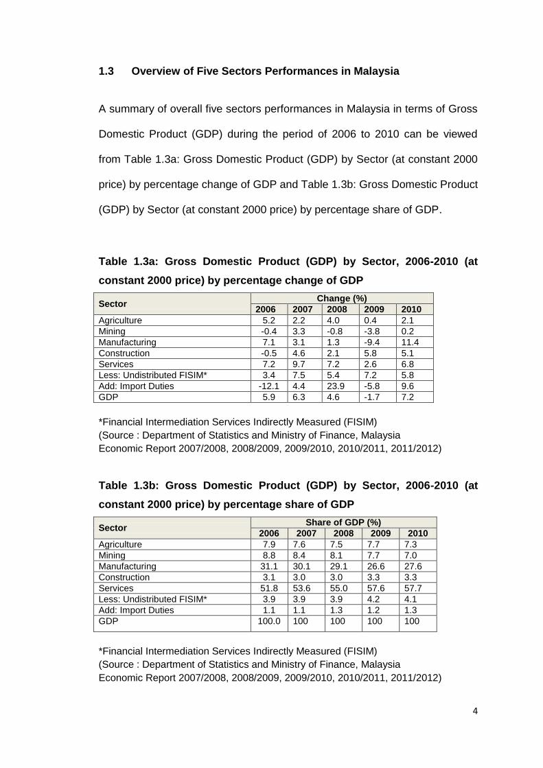
A summary of overall five sectors performances in Malaysia in terms of Gross

Domestic Product (GDP) during the period of 2006 to 2010 can be viewed

from Table 1.3a: Gross Domestic Product (GDP) by Sector (at constant 2000

price) by percentage change of GDP and Table 1.3b: Gross Domestic Product

(GDP) by Sector (at constant 2000 price) by percentage share of GDP.

Table 1.3a: Gross Domestic Product (GDP) by Sector, 2006-2010 (at

constant 2000 price) by percentage change of GDP

Sector Change (%)

2006 2007 2008 2009 2010

Agriculture 5.2 2.2 4.0 0.4 2.1

Mining -0.4 3.3 -0.8 -3.8 0.2

Manufacturing 7.1 3.1 1.3 -9.4 11.4

Construction -0.5 4.6 2.1 5.8 5.1

Services 7.2 9.7 7.2 2.6 6.8

Less: Undistributed FISIM* 3.4 7.5 5.4 7.2 5.8

Add: Import Duties -12.1 4.4 23.9 -5.8 9.6

GDP 5.9 6.3 4.6 -1.7 7.2

*Financial Intermediation Services Indirectly Measured (FISIM)

(Source : Department of Statistics and Ministry of Finance, Malaysia

Economic Report 2007/2008, 2008/2009, 2009/2010, 2010/2011, 2011/2012)

Table 1.3b: Gross Domestic Product (GDP) by Sector, 2006-2010 (at

constant 2000 price) by percentage share of GDP

Sector Share of GDP (%)

2006 2007 2008 2009 2010

Agriculture 7.9 7.6 7.5 7.7 7.3

Mining 8.8 8.4 8.1 7.7 7.0

Manufacturing 31.1 30.1 29.1 26.6 27.6

Construction 3.1 3.0 3.0 3.3 3.3

Services 51.8 53.6 55.0 57.6 57.7

Less: Undistributed FISIM* 3.9 3.9 3.9 4.2 4.1

Add: Import Duties 1.1 1.1 1.3 1.2 1.3

GDP 100.0 100 100 100 100

*Financial Intermediation Services Indirectly Measured (FISIM)

(Source : Department of Statistics and Ministry of Finance, Malaysia

Economic Report 2007/2008, 2008/2009, 2009/2010, 2010/2011, 2011/2012)

5

Based on the above Table 1.3a, overall, Malaysia’s GDP had increased

slightly from 5.9% in 2006 to 6.3% in 2007. However, from year 2008 to 2009,

the country’s GDP had declined to 4.6% and negative 1.7% in 2008 and 2009

respectively, which was mainly due to the global economic crises experienced

in year 2008 (Economic Report 2010/2011). In year 2010, Malaysia’s

economy had revived and reported a GDP growth of 7.2% (Economic Report

2011/2012). From Table 1.3b, noted that services sector is the key driver of

economic growth, which consists of more than 50% of the country’s GDP and

had shown an increasing trend from year 2006 onwards to 57.7% shares of

GDP in 2010 (Economic Report 2011/2012). However, noted that the

manufacturing sector performance had showed a declining trend from 31.1%

share of GDP in 2006 to 26.6% share of GDP in 2009 (Economic Report

2010/2011). However, in 2010, the manufacturing sector’s performance had

improved slightly by 1% to 27.6% share of GDP in 2010 (Economic Report

2011/2012).

1.3.1 Overview of Services and Manufacturing sector performance

Based on Bank Negara Malaysia’s (BNM) Annual Report 2006 and Economic

Report 2007/2008, Malaysia’s economy had registered a real gross domestic

product (GDP) growth of 5.9% in year 2006, which was mainly contributed by

strong internal demand and continuous healthy exports. Based on Table 1.3a,

the services sector had spearheaded the overall economy by recorded a 7.2%

growth in GDP, followed by 7.1% growth in GDP from manufacturing sector

which revealed a slight structural movement in Malaysian economy from

manufacturing to services (Economic Report 2007/2008).

6

Based on the Economic Report 2007/2008, the services sector comprises of

intermediate services, final services and government services. The

intermediate services consist of transport and storage, communication,

finance and insurance, real estate and business services sub-sectors, while

final services is represented by utilities, wholesale and retail trade,

accommodation and restaurant, and other services sub-sectors. Meanwhile,

based on the Economic Report 2007/2008, the manufacturing production

index performance is divided into export-oriented industries and domestic-

oriented industries.

In 2006, services sector contributed 51.8% share of GDP while manufacturing

sector consists of 31.1% share of GDP. Based on the services sector

performance, the top two services sub-sectors are wholesale and retail trade

that had expanded by 7.1% of GDP with 11.6% share of GDP in services

sector, and followed by finance and insurance sub-sectors generated a 7.7%

growth in GDP with 10.2% share of GDP in services sector (Economic Report

2007/2008). The increase in finance and insurance sub-sector is due to

expansion in consumer credit, investment for businesses, Islamic financing

and higher demand for investment-linked, medical and health insurance

products. Meanwhile, the growth in wholesale and retail trade sub-sector is

mainly due to strong private consumption, increase in disposable income,

expansion in retail activity and promotion of tourism industry, which is in

conjunction with Visit Malaysia Year 2007 (Economic Report 2007/2008).

7

The manufacturing sector reported a growth of 7.1% with 31.1% shares to

GDP in 2006 (Economic Report 2007/2008), which is strengthen by the

worldwide electronics upward trend, higher requirement for resource-based

industries such as petroleum, rubber and off-estate processing that enjoyed

increase in export prices and enhancement in performance of domestic-

oriented industries by 7.2% in 2006, which is attributed by construction related

industries known as iron and steel, non-metallic products and fabricated metal

products (BNM Annual Report 2006).

Despite vulnerable economic environment, Malaysia’s GDP increased by

6.3% in 2007, which was attributed by healthy domestic demand especially in

private consumption and investment activities (BNM Annual Report 2007).

The services sector maintains as the main generator of economic growth by

reporting a 9.7% growth in GDP, which accounted for 53.6% share of GDP in

2007 (Economic Report 2008/2009). The growth was mainly due to increase

in domestic demand and activities related to tourism in tandem with Visit

Malaysia Year 2007. Reportedly, the major contributors to robust performance

of services sector comes from real estate and business services; finance and

insurance; communication; and wholesale and retail trade sub-sectors (BNM

Annual Report 2007). For manufacturing sector, it had reported moderate

growth of 3.1% in 2007 (2006: 7.1%) with its contribution to overall GDP

decline slightly to 30.1% shares (Economic Report 2008/2009) as a result of

decline in demand for electronics and electrical (E&E) industry (BNM Annual

Report 2007). However, the moderate growth has been mitigated by broad

manufacturing base and increase in demand for local and resource-based

8

industries such as rubber, petroleum, chemicals and chemical products from

Asia-Pacific region (BNM Annual Report 2007).

According to BNM’s annual report 2008, Malaysia had recorded GDP growth

of 4.6% in 2008 despite experienced global economic crisis in the second half

of 2008, which had impacted the country’s export as well as resulted in lower

private investment activities. Services sector had remained as the main

contributor towards GDP by reporting growth rate of 7.2% of GDP and 55%

share of GDP in 2008. The services sector had maintained as a leader in

economic growth due to increase in demand domestically, growth in trade and

tourism activities via opening up more hypermarkets and retail outlets in

conjunction to Visit Malaysia Year and Mega Sales carnivals being extended,

which encouraged public spending. However, manufacturing sector had

showed a drop in GDP’s growth of 1.3% in 2008 (2007: 3.1%), which is

motivated by domestic-oriented industries in view that export-oriented

industries had contracted significantly arising from decline in global demand

specifically in the E&E industry. In spite of that, manufacturing sector stood as

second highest contribution towards the country’s GDP by recording a 29.1%

share of GDP in 2008 (2007: 30.1%).

In 2009, Malaysia economy had shrank by 1.7% in 2009 as a result of the

global economy slowdown experienced in 2008. The domestic economy

declined by 6.2%, while exports and industrial production registered double-

digit decrease due to deteriorating demand globally (BNM Annual Report

2009). In first quarter of 2009, the services sector reported a moderate drop in

9

performance arising from deterioration from services sub-sectors associated

to manufacturing and trade activities. However, from second quarter onwards,

the services sector had shown an improvement in performance which is

derived from services sub-sectors that relied on domestic economy and

activities associated to finance and capital market. For manufacturing sector,

it was severely impacted by global economic slowdown which recorded a

decline of 22.8% in 2009, especially in the electronics and electrical products

(E&E) cluster in the export-oriented industry. However, situation improved

gradually from second quarter onwards with positive growth reported in

production in the fourth quarter of 2009.

There are three policy measures being implemented in order to mitigate the

global economic recession such as two fiscal economic stimulus packages

totalling RM67 billion which aims to support domestic demand, minimizing the

effect of global economic slowdown on impacted sectors as well as to reduce

unemployment rate in the country. The second policy being implemented

refers to monetary stimulus package such as reduction in overnight policy rate

by 150 basis points to 2.0% between November 2008 and February 2009;

and reduction in statutory reserve requirement by 300 basis points to 1.0% in

order to lessen the intermediary cost, mitigates the slowdown in external

demand and to enhance consumer and business outlooks domestically.

Meanwhile, comprehensive measures are also being introduced to enable

continuous access to financing such as guarantee scheme for SMEs and

businesses (BNM Annual Report 2009).

10

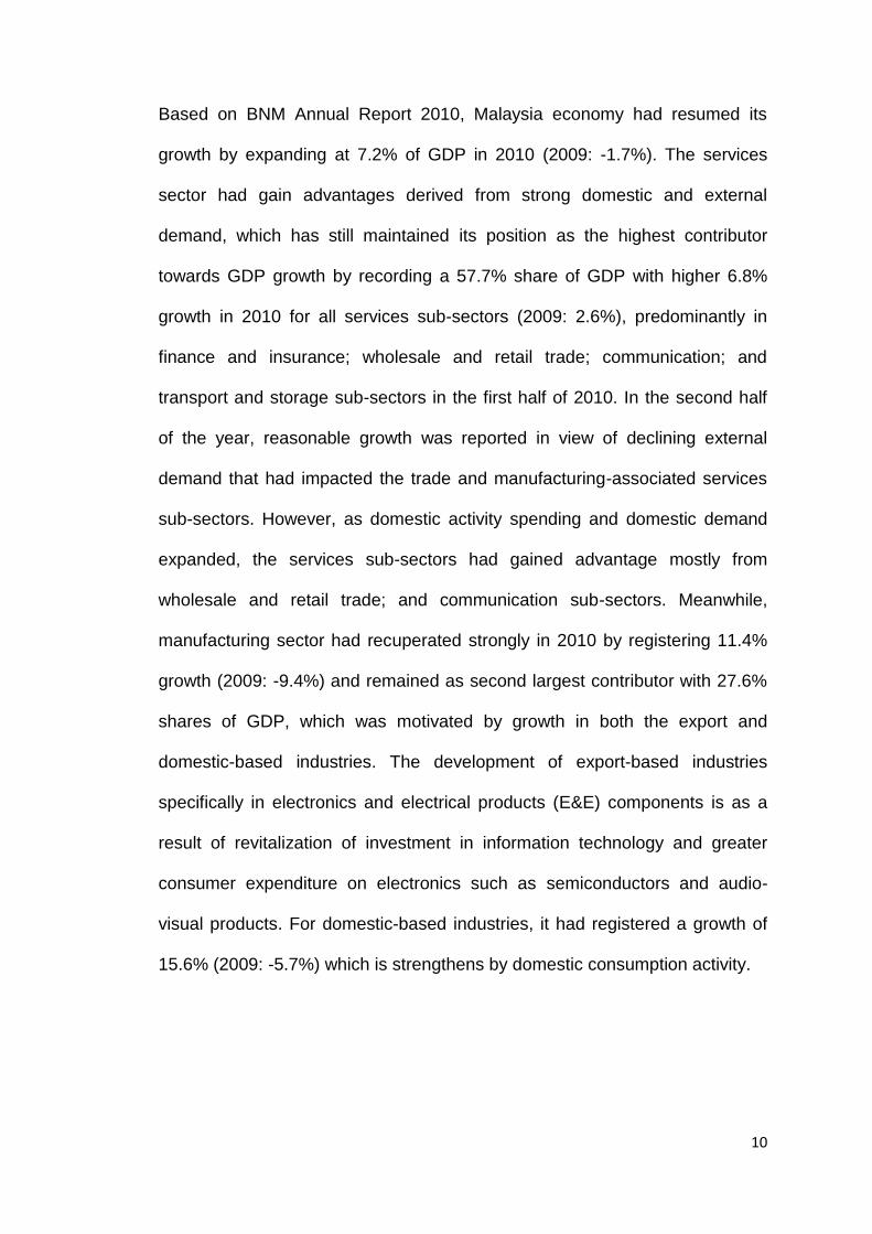
Based on BNM Annual Report 2010, Malaysia economy had resumed its

growth by expanding at 7.2% of GDP in 2010 (2009: -1.7%). The services

sector had gain advantages derived from strong domestic and external

demand, which has still maintained its position as the highest contributor

towards GDP growth by recording a 57.7% share of GDP with higher 6.8%

growth in 2010 for all services sub-sectors (2009: 2.6%), predominantly in

finance and insurance; wholesale and retail trade; communication; and

transport and storage sub-sectors in the first half of 2010. In the second half

of the year, reasonable growth was reported in view of declining external

demand that had impacted the trade and manufacturing-associated services

sub-sectors. However, as domestic activity spending and domestic demand

expanded, the services sub-sectors had gained advantage mostly from

wholesale and retail trade; and communication sub-sectors. Meanwhile,

manufacturing sector had recuperated strongly in 2010 by registering 11.4%

growth (2009: -9.4%) and remained as second largest contributor with 27.6%

shares of GDP, which was motivated by growth in both the export and

domestic-based industries. The development of export-based industries

specifically in electronics and electrical products (E&E) components is as a

result of revitalization of investment in information technology and greater

consumer expenditure on electronics such as semiconductors and audio-

visual products. For domestic-based industries, it had registered a growth of

15.6% (2009: -5.7%) which is strengthens by domestic consumption activity.

11

1.4 Statement of the Problem

Malaysia has undergone a tremendous development from an agricultural and

commodity-based economy towards a middle-income nation by registering

real Gross Domestic Product (GDP) growth of an average of 5.8% per annum

from 1991 to 2010 (Tenth Malaysia Plan, 2011-2015). There are three

important nationwide policy structures such as New Economic Policy (NEP),

1971-1990, National Development Policy (NDP), 1991-2000 and National

Vision Policy (NVP), 2001-2010 being implemented with the purpose of

achieving a developed nation status by year 2020 as in line with Vision 2020.

With the introduction of the Ninth Malaysia Plan, 2006 to 2010, one of the

directions is to shift the economy upward the value chain via expansion in the

productivity, competitiveness and value added activities of agriculture,

manufacturing, and services sectors (Ninth Malaysia Plan). This is also in

tandem with the implementation of Malaysia’s Third Industrial Master Plan

(IMP3) from year 2006 to 2020 which focuses on transforming and innovating

the manufacturing and services sector (Third Industrial Master Plan).

Furthermore, there are several incentives introduced during Ninth Malaysia

Plan to lessen the cost of operating business such as the removal of Foreign

Investment Committee (FIC) guidelines to attract more foreign and domestic

investment, simplify the business licences and registration process, and

liberalisation policy initiated for conventional and Islamic finance sector, which

there is liberalisation for a total of 27 services subsectors with no equity

requirement (Tenth Malaysia Plan). Based on Third Industrial Master Plan,

there are also direct and indirect tax incentives introduced for sectors such as

12

manufacturing, agriculture, tourism (together with hotel) which also caters for

research and development (R&D) activities.

In year 2008, the global economic slowdown and Malaysia’s open economy

policy had resulted in the country’s GDP declined by 1.7% in 2009 and

deterioration in industrial production and manufacturing exports as it relied

heavily on global demand (Tenth Malaysia Plan). However, despite the global

economic slowdown, based on Economic Report 2010/2011, the services

sector had experienced a positive GDP’s growth rate of 2.6% in 2009 which

represents 57.6% share of GDP in 2009 as compared to manufacturing sector

reported a negative 9.4% growth in GDP with 26.6% share of GDP in 2009.

Therefore, in this study, the main reason for services and manufacturing

sectors being analysed is due to services sector has surpassed the

performance of the manufacturing sector as it represents 57.7% shares of

Malaysia’s GDP in 2010 (the highest contributor for GDP), as compared to

manufacturing sector which reported as the second highest contributor with

27.6% shares of Malaysia’s GDP in 2010 (Economic Report 2011/2012).

Hence, it is vital to analyse on the performance of firms in both the services

and manufacturing sectors as it constitutes 85.3% shares of Malaysia’s GDP

in 2010. Furthermore, this is also in tandem with the emphasise placed by

government via Malaysia’s Third Industrial Master Plan (IMP3), 2006- 2020,

which also coincides with the Ninth Malaysia Plan, 2006-2010, which one of

the thrusts of the National Mission is to shift the economy upward the value

chain by increasing the value added of manufacturing, services and

13

agriculture sector. In addition, based on Tenth Malaysia Plan, services sector

is projected to be the main foundation of economic development as a result of

growth in finance and business services, wholesale and retail trade, hotel and

restaurants, transport and communication subsectors (Tenth Malaysia Plan).

There are various factors being analysed by researchers as the determinants

of profitability of a firm, which include working capital management. In

addition, there is also lack of study being conducted on factors contributing

towards the profitability of services sector, as compared to determinants of

profitability for manufacturing or industrial firms (McDonald, 1999; Leachman,

Pegels and Shin, 2005). Hence, in view that services sector had led the

economic performance in Malaysia, it is imperative that evaluation on the

factors that contribute towards the firm’s profitability in services sector being

analysed in terms of the effects of working capital management.

In view that one of the financial considerations in business is WCM, there are

various empirical research being conducted by researchers on the effects of

WCM on profitability of firms (Shin and Soenen, 1998; Deloof, 2003; Lazaridis

and Tryfonidis, 2006). However, in Malaysia, the WCM topic has not been

extensively being research as compared to other corporate finance studies

such as capital structure and capital budgeting, due to WCM is perceived as

investment and financing in short time interval (Zariyawati, Taufiq, Annuar and

Sazali, 2010). This is also due to short-term financial management has been

regarded as less significant and often being overlooked by researchers, which

give more emphasis to other parts of corporate finance and investment

14

despite WCM takes up substantial share of time of the finance managers

(Nasruddin, 2006).

Furthermore, based on the researchers’ findings, the results are inconsistent

for different studies conducted. In addition, despite various studies being

undertaken to investigate on the effect of working capital management on the

profitability of firms, the results revealed mixed findings and different

researchers used different methodology or approach in measuring the

working capital management, such as cash conversion cycle (Padachi, 2006),

current ratio (Nor Edi Azhar and Noriza, 2010) and net trade cycle (Shin and

Soenen, 1998; Erasmus, 2010). Besides that, in Malaysia context, there is

limited study being explored in analysing on the effect of working capital

management on the firm’s profitability especially in the services sector, which

is currently the country’s highest contributor in terms of GDP in 2010 (57.7%).

Furthermore, there is also separate analysis being conducted on the effect of

working capital management components and working capital management

policy on the profitability of the firms by the researchers.

Therefore, in this study, we would like to investigate on the effectiveness of

the policy implemented during the Ninth Malaysia Plan, 2006-2010, and Third

Industrial Master Plan, 2006-2020 by analysing on the WCM components and

WCM policies that affect the firm’s performance in terms of profitability of the

services and manufacturing sector during the period of 2006 to 2010. This

study is also to fill up the gap by investigating on the effect of working capital

management on the firm’s profitability in services sector that is represented by

trading/services sector and manufacturing sector which is represented by

15

industrial products sector during the period of 2006 to 2010, which is also in

tandem with the implementation of the Ninth Malaysia Plan, 2006-2010 and

Third Industrial Master Plan (IMP3) period, 2006-2020.

1.5 Research Questions

This study attempts to fill up the gap of working capital management studies

by focusing specifically in services sector and as comparison to the

manufacturing sector. Based on the problem statement highlighted, the result

of this study is to find out answer for the following identified research

questions:-

i) What is the effect of working capital management components towards the

firm’s profitability in services and manufacturing sectors during the

implementation of the Ninth Malaysia Plan (9MP) and Third Industrial

Master Plan (IMP3) from period of 2006 to 2010?

a) How does number of days Accounts Receivable (ARD) affects the

profitability of the services and manufacturing firms in Malaysia?

b) How does number of days Inventories (INV) affects the profitability of

the services and manufacturing firms in Malaysia?

c) How does number of days Accounts Payable (AP) affects the

profitability of the services and manufacturing firms in Malaysia?

d) How does cash conversion cycle (CCC) affects the profitability of the

services and manufacturing firms in Malaysia?

ii) What is the working capital management policy being adopted, whether

aggressive or conservative Working Capital Investment Policy (WCIP) or

16

Working Capital Financing Policy (WCFP) being adopted by services and

manufacturing sectors during the implementation of the Ninth Malaysia

Plan and Third Industrial Master Plan (IMP3) from period of 2006 to 2010?

iii) What is the difference in terms of profitability for services sector as

compared to manufacturing sector during the implementation of the Ninth

Malaysia Plan and Third Industrial Master Plan (IMP3) from period of 2006

to 2010?

1.6 Research Objectives

The research objectives of this study are as follow:-

i) To examine the effect of working capital management components on the

profitability of services and manufacturing firms in Malaysia during the

implementation of the 9MP and IMP3 from period of 2006 to 2010.

a) To investigate the effect of number of days Accounts Receivable (ARD)

towards the profitability of the services and manufacturing firms in

Malaysia.

b) To investigate the effect of number of days Inventories (INV) towards

the profitability of the services and manufacturing firms in Malaysia.

c) To investigate the effect of number of days Accounts Payable (AP)

towards the profitability of the services and manufacturing firms in

Malaysia.

d) To investigate the effect of cash conversion cycle (CCC) towards the

profitability of the services and manufacturing firms in Malaysia.

17

ii) To determine on the working capital management policy, whether

aggressive or conservative Working Capital Investment Policy (WCIP) or

Working Capital Financing Policy (WCFP) being adopted by services and

manufacturing sectors during the implementation of the Ninth Malaysia

Plan and Third Industrial Master Plan (IMP3) from period of 2006 to 2010.

iii) To investigate if there is any significant difference in profitability between

services and manufacturing sector during the implementation of the Ninth

Malaysia Plan and Third Industrial Master Plan (IMP3) from period of 2006

to 2010.

1.7 Purpose and Significance of the Study

The importance of conducting this study is it allows firm managers to expand

their learning curve to reduce the possibility of default, especially in turbulent

time; in view that working capital management has influence on the

profitability performance of the firms.

Furthermore, this study is also of importance for practitioner, policy maker,

academician and firm managers with regards to issue associated with the

effect of working capital management on profitability of firm, as it enables

minimisation of firm’s cost of finance and further planning being conducted in

order to maximise firm’s profitability and shareholders’ wealth.

18

1.8 Scope of the Study

This study focuses on services and manufacturing firms that are continuously

listed in the Main Market of Bursa Malaysia that are represented under

trading/services and industrial products sectors from year 2006 to 2010 for

five years period. In this study, analysis is done based on secondary data

obtained from Datastream 5.1 terminal.

1.9 Organisation of the Study

This research project will be organised into five chapters as follows:-

Chapter 1 : Introduction and overview of the study.

Chapter 2 : Literature review on the working capital management (WCM),

the effect of WCM components and WCM policies towards the

profitability of the firms in services and manufacturing sectors.

Chapter 3 : Research Methodology, which discussed more on research

design, research framework, data collection, development of

hypotheses and data analysis.

Chapter 4 : Research Results and Analysis, which refers to the testing of

hypotheses and discussion of the results obtained from panel

data regression analysis.

Chapter 5 : Conclusion and recommendations for future research, which

also discussed on the limitations and implications of the study.

19

CHAPTER 2 : LITERATURE REVIEW

2.0 Introduction

The objective of this chapter is to critically review past theoretical and

empirical study conducted with regard to working capital management. There

are several studies being carried out by researchers to provide insights on the

effect of working capital management towards the firm’s profitability.

This chapter starts off with the brief description on the role of working capital

management (WCM), followed by optimal WCM, theories of WCM and WCM

policy, as well as discussed on the trade-off between liquidity and profitability.

Past literature reviews in relation to the effect of WCM on profitability of firms

are also elaborated further by dividing the area of study into developed

countries, developing countries and in Malaysia’s perspectives.

2.1 Role of Working Capital Management (WCM)

Traditionally, corporate finance study has emphasised on long-term financing

decision, particularly in capital budgeting, capital structure and dividends

(Nobanee, Abdullatif and AlHajjar, 2011), despite the fact that working capital

management (WCM) constitutes as one of the financing considerations that a

finance manager need to determine, besides capital budgeting and capital

structure (Ross, Westerfield and Jordan, 2010). In view of the global financial

crisis experienced in 2008, WCM topic has started been given a priority as it

relates to managing the firm’s resources in order to meet the daily operation

of the business (Charitou, Elfani and Lois, 2010). Furthermore, according to

20

Deloof (2003) and Gill, Biger and Mathur (2010), managing working capital is

crucial in view that it has a major and direct influence on firm’s profitability.

Working capital management (WCM) is associated with managing short-term

financial aspects and it is related to net working capital that involves in

determination of financing considerations in short duration, which is within a

year or less (Ross, Westerfield, Jordan, 2010). Generally, WCM is simply

indicated as managing current assets and current liabilities (Raheman and

Nasr, 2007). Working capital refers to short term or current assets that are

reflected on firm’s balance sheet such as trade receivables and inventory,

meanwhile computation of net working capital exclude current liabilities, such

as trade payables from the current assets (Eljelly, 2004; Erasmus, 2010). The

net working capital plays an important role as it determines the availability of

funds in meeting the daily operations of the firm and has impacts towards

generating firm’s profitability and shareholders’ value (Eljelly, 2004).

In addition, based on study conducted by Smith (1980), WCM demonstrates a

significant function in view of the trade-off between liquidity and profitability

that has impacts on firm’s profitability, risk as well as the value of the

corporation. Thus, effective utilisation of investment in working capital is vital

as an overinvestment in working capital that is not utilised may lead to lower

firm’s value, while working capital that is underinvested may resulted in firm

facing liquidity difficulty. Hence, as a consequence of not having sufficient

investment in cash, trade receivables or inventory, it is challenging for firm to

21

operate its day-to–day operations which may resulted in sales decline and

affected the firm’s profitability (Erasmus, 2010).

Working capital management (WCM) which is also known as liquidity

management is essential in determining the success of a firm as it involves

organization of current assets and current liabilities (Uyar, 2009). Hence,

should the firm unable to organise its liquidity level, this means that its current

asset unable to cover its current liabilities such as short term debts. Thus, firm

may resort to external funding which has the possibility of incurring higher

cost of financing that may lead to lower profitability (Uyar, 2009) and

possibility of becoming insolvency and bankruptcy due to poor credit position

(Nasruddin, 2006). As highlighted by Eljelly (2004), efficient liquidity

management relates to organising and monitoring of current assets and

current liabilities that allow elimination of risk for firms that unable to meet its

short-term commitment and at the same time, preventing excessively

investment in these assets.

According to Hill and Sartoris (1995), the firm’s value can be improved further

by having adequate liquidity position as it enable smooth operation of

business, enhancement of shareholders’ value and offers flexible financial

choices at an attractive cost. Furthermore, creditors are also concerned with

the firm’s liquidity position due to it reflects whether the firm’s current assets

able to deal with its present current liabilities (Smith and Begemann, 1997).

Therefore, WCM study is utmost important in managing the daily operation of

the firm.

22

2.2 Optimal Working Capital Management

The key objective of managing working capital is to achieve an optimum level

in each segments of the working capital, such as receivables, inventory and

payables (Filbeck and Krueger, 2005, Afza and Nazir, 2007) that enables

equilibrium to be maintain between risk and efficiency (Afza and Nazir, 2007).

Thus, finance manager has emphasised in maintaining optimal current assets

and current liabilities in order to achieve optimal working capital position

(Lamberson, 1995) and maximisation of firm’s value (Howorth and Westhead,

2003, Deloof, 2003, Afza and Nazir, 2007).

Adequacy of liquidity level is important in order for firm to improve its value as

it allows for contingency purposes in operations and offers flexible financing at

a lower cost (Eljelly, 2004). In addition, Smith (1980) had highlighted on the

WCM goals, which involves the trade-off between liquidity and profitability.

Thus, firm needs to balance its liquidity and profitability level as if firm is

wholly focussing in profit maximisation, the sufficiency of the firm’s liquidity

position will be affected and vice versa (Nasruddin, 2006).

2.3 Operating Cycle and Cash Conversion Cycle

The operating cycle of a business refers to a period of time between inventory

arrivals until the cash receipts derived from the receivables. Sometimes,

operating cycle also include time from placement of order until arrival of the

stock (Ross, Westerfield and Jaffe, 2005). Moss and Stine (1993) defined

operating cycle as the total of average number of days required to purchase

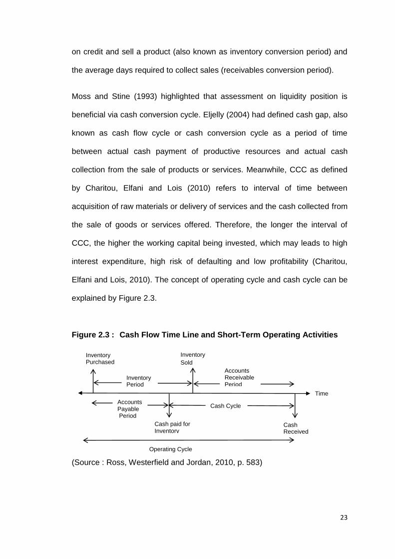
23

on credit and sell a product (also known as inventory conversion period) and

the average days required to collect sales (receivables conversion period).

Moss and Stine (1993) highlighted that assessment on liquidity position is

beneficial via cash conversion cycle. Eljelly (2004) had defined cash gap, also

known as cash flow cycle or cash conversion cycle as a period of time

between actual cash payment of productive resources and actual cash

collection from the sale of products or services. Meanwhile, CCC as defined

by Charitou, Elfani and Lois (2010) refers to interval of time between

acquisition of raw materials or delivery of services and the cash collected from

the sale of goods or services offered. Therefore, the longer the interval of

CCC, the higher the working capital being invested, which may leads to high

interest expenditure, high risk of defaulting and low profitability (Charitou,

Elfani and Lois, 2010). The concept of operating cycle and cash cycle can be

explained by Figure 2.3.

Figure 2.3 : Cash Flow Time Line and Short-Term Operating Activities

(Source : Ross, Westerfield and Jordan, 2010, p. 583)

Inventory Period

Accounts Receivable Period

Accounts Payable Period

Cash Received

Inventory

Sold

Cash paid for Inventory

Inventory Purchased

Time

Operating Cycle

Cash Cycle

24

According to Ross, Westerfield and Jordan (2010), operating cycle refers to

the length of time from procurements of inventory until cash from receivables

is accepted. Meanwhile, cash cycle demonstrates the period of time between

cash payment and receiving collection of cash (Ross, Westerfield and Jordan,

2010).

Based on Figure 2.3 above, the difference between operating cycle and cash

cycle is summarised as below:-

Firms can achieved greater sales by maintaining higher inventory level in

order to mitigate the risk of insufficient supply of stock and liberal trade credit

policy may motivate further sales as it enable evaluation of product prior to

payment (Long, Malitz and Ravid, 1993; and Deloof and Jegers, 1996).

2.4 Theories of Working Capital Management

Based on studies conducted by Moss and Stine (1993); Lancaster et al.

(1999); Farris and Hutchison (2002), there are two distinctive aspects of

working capital management, which comprise of static or dynamic viewpoints.

The static point of view reflects conventional measurement of liquidity ratios,

for example current ratio and quick ratio measured at a particular point in time

on balance sheet (Moss and Stine, 1993).

Operating Cycle = Inventory period + Accounts receivable period

Cash Cycle = Operating Cycle – Accounts payable period

(Source : Ross, Westerfield and Jordan, 2010, p.582)

25

Although working capital and liquidity ratios are part of liquidity measurement,

they are not left without critics (Eljelly, 2004). As highlighted by Finnerty

(1993), conventional liquidity ratios comprise of current ratio or quick ratio

which consist both liquid financial assets and operating assets. Hence, as

operating assets are held up in operations, it is deemed as not beneficial in

terms of on-going concern opinion. Furthermore, current and quick ratios are

also not efficient in view of their static nature and incapability of forecasting

future cash flows and liquidity (Kamath, 1989). Thus, from the weaknesses

identified for working capital and liquidity ratios, net cash conversion cycle or

also known as cash gap has been introduced as alternative to liquidity

measurement (Gitman, 1974; Richard and Laughlin, 1980; Boer, 1999 and

Gentry et al., 1990) as it is more realistic based on the dynamic nature of cash

cycles (Eljelly, 2004). Furthermore, the dynamic view computes liquidity of

firm’s operations continuously, for instance cash conversion cycle that

involves both balance sheet and income statement with time perspective

(Jose et al., 1996).

Richards and Laughlin (1980) had long established the principle of working

management by initiating the idea of cash conversion cycle as a strong

performance indicator for management of firm’s working capital. Cash

conversion cycle (CCC) or cash gap computes the period of time between

actual cash expenses and actual cash receipts from the sale of products or

services (Eljelly, 2004).

26

2.5 Working Capital Management (WCM) Policy

The working capital management (WCM) policy is divided into working capital

investment policy (WCIP) and working capital financing policy (WCFP). A firm

may select an aggressive WCIP, which adopts a lower ratio of total current

assets to total assets or select an aggressive WCFP policy that focus in

maintaining a higher ratio of total current liabilities to total assets (Afza and

Nazir, 2007). On the other hand, an excess of current assets has an inverse

relationship with firm’s profitability, while lower level of current assets caused

lower liquidity position and risk of insufficiency of stock which resulted in

challenges to support smooth operation of business (Van Horne and

Wachowicz, 2004).

The trade-off between various policies of working capital has long been

debated (Pinches, 1991, Brigham and Ehrhardt, 2004, Moyer et. al., 2005,

Gitman, 2005). An aggressive working capital policy is related to higher return

and higher risk, which is contrary to conservative working capital policies

which emphasis on minimising risk and return (Gardner et al. 1986, Weinraub

and Visscher, 1998). It was found that the higher the investment in current

assets, the lower the risk and profitability incurred. Based on the empirical

findings by Carpenter and Johnson (1983), there is no linear relationship

found between current assets and systematic risk of US firms.

Weinraub and Visscher (1998) had conducted study on both policies of

aggressive and conservative WCM by analysing quarterly data of ten various

industries of US firms, during the period of 1984 to 1993. He concluded that

there is a balance between adaptations of aggressive working capital on one

27

hand with a conservative policy at the other hand. Thus, in this study, it is

imperative that study is being conducted to also analyse on the effect of

working capital management policy towards the firm’s profitability.

2.6 Trade-off between Liquidity and Profitability

The working capital of the firm relates to liquidity management, which consists

of current assets as indicated on balance sheet of the firm, meanwhile net

working capital disregards the current liabilities (Eljelly, 2004). Hence, in

ensuring effective liquidity management of the firms, planning and monitoring

of current assets and current liabilities are important to meet short-term

obligations and to reduce extreme investment in these assets, as it has

impact on the profitability and shareholders’ value of the firms (Eljelly, 2004).

According to Smith (1980), there is a trade-off between liquidity and

profitability, which are the dual goals of working capital management. In view

that management of working capital has a significant effect on both liquidity

and profitability of the firms, it is important that firms attain an optimal level in

efficiency of the working capital management (Nasruddin, 2006). Hence, there

should be a balance in liquidity position of the firms that is neither excess nor

insufficient. This is due to extreme liquidity level indicates growth of idle funds

that disallow firms to enjoy better profit as the reserves of the firms are held

up in liquid assets and are not available to be used in operating or investing

activities that are able to gain higher profitability. Meanwhile, inadequate

liquidity level has an impact on the repayment capability of the firms and

28

resulted in declining credit position and possibility of becoming insolvent and

bankrupt (Nasruddin, 2006). Therefore, by focussing solely on liquidity may

lessen the prospective profitability of the firms, while on the other hand, fully

prioritising on profit maximization will reduce the opportunity of having

sufficient liquidity for the firms (Nasruddin, 2006). Furthermore, based on the

theory of risk return, firms with higher liquidity position may faced lower risk

and enjoys lower profitability, as compared to firms with low liquidity level that

may incur higher risk, which resulted in higher return (Niresh, 2012). Hence,

firms need to achieve a balance between liquidity and profitability in the daily

operations of their business.

In addition, shorter cash conversion cycle is preferred due to longer cash

cycle or cash gap incurs higher external financing cost in terms of explicit and

implicit costs that affected the profitability of the firms (Eljelly, 2004). Loeser

(1988) had highlighted on the significance of liquidity management by

reducing the cash conversion cycle via evaluating the accounts receivable

and unbilled revenue at prime rate of the interest rate, in order for receivables

collected promptly to reduce the cash gaps. Hence, finance managers of the

firms also need to ensure all invoicing, collections and payables systems are

operated effectively (Fraser, 1998).

Furthermore, there are many researchers conducted study on the trade-off

between liquidity and profitability. However, noted that the result varies based

on the study undertaken, which the findings are discussed further and

segregated according to developed and developing countries as well as

Malaysia perspective as per items 2.7, 2.8 and 2.9.

29

2.7 Past studies on Working Capital Management and Profitability in

Developed countries

Shin and Soenen (1998) had examined on the relationship between the firm’s

net-trade cycle and profitability via correlation and regression analysis. Based

on a Compustat sample of 58,985 listed American firm years during the period

of 1975 to 1994, they found a strong negative association between the

interval of the firm's net-trade cycle and profitability. The firm’s profitability is

measured by operating income plus depreciation related to total assets and to

net sales. Net- trade cycle (NTC) was used as a measurement for efficiency

of WCM instead of CCC due to each of the three segments in WCM such as

number of days inventories, accounts receivable and accounts payable are

measured based on percentage of sales and assuming other things being

equal (ceteris paribus conditions). This is unlike CCC which has various

denominators for the three segments and hence, projection on the additional

working capital requirement for the corporation is difficult. Their findings also

revealed that shorter NTC leads to higher present value of net cash flow and

higher shareholders value. Thus, if the firm has shorter NTC, it means that the

firm manages its working capital efficiently as the firm requires less external

financing which denote an improved financial performance.

Deloof (2003) had investigated on the relationship between working capital

management and firms’ profitability of 1,009 large Belgian non-financial

corporations from 1992 to 1996. His results revealed a significant negative

relationship between gross operating income with the number of days

accounts receivable, inventories and accounts payable. Hence, from the

30

result obtained, it is proposed that shareholders value can be enhanced by

maintaining a minimum number of days accounts receivable, inventories and

accounts payable. Noted that firm’s profitability is being represented by gross

operating income instead of return on assets as for firm that has mostly

financial assets on its balance sheet, the operating activities had less

influence to the return on assets.

Lazaridis and Tryfonidis (2006) had studied on the relationship between

working capital management and profitability of 131 corporations listed in

Athens Stock Exchange during time interval of 2001 to 2004. Their results

revealed that there is a negative association between profitability, which is

computed using gross operating profit, with cash conversion cycle as indicator

for determining the effectiveness of working capital management. Hence, it is

suggested that the firm’s profitability can be enhanced by managing the cash

conversion cycle and maintain its segments such as accounts receivables,

accounts payables and inventory at an optimal stage. Gross operating profit

represents the measurement for profitability instead of earnings before

interest tax depreciation amortization (EBITDA) or pretax profit or net profit

due to their intension of establishing an association between accomplishment

or collapse of a business operation with operating ratio and associate it further

with other operating variables such as cash conversion cycle. Furthermore,

financial assets are deducted from total assets in order to eliminate the

involvement of finance activity from operation activity, which may affect firm’s

profit.

31

Gill, Biger and Mathur (2010) had broadened the study conducted by

Lazaridis and Tryfonidis (2006) with regard to the relationship between

working capital management and profitability. They have conducted an

investigation on the relationship between working capital management and

profitability of a sample of 88 American manufacturing firms listed on the New

York Stock Exchange for a period of 3 years from 2005-2007 by adopting

correlational and non-experimental research design. Based on their

observation, there is a negative association between profitability, computed

via gross operating profit and average days of accounts receivable. They also

found that there is a positive relationship between cash conversion cycle and

profitability, while negative relationship discovered between accounts

receivables and firm’s profitability implied that for less profitable corporations,

they will reduce their accounts receivables in order to shorten the cash gap in

the CCC. Meanwhile, there is no significant relationship identified between

firm size and gross operating profit ratio. Furthermore, it is suggested that the

firm’s profitability and shareholders value can be enhanced by managing their

CCC efficiently and by maintaining their accounts receivables at an optimum

position.

Nobanee, Abdullatif and AlHajjar (2011) had studied on the relationship

between firm’s cash conversion cycle and its profitability for 34,771 Japanese

non-financial firms listed on the Tokyo Stock Exchange from the period of

1990 to 2004. By using dynamic panel data analysis, they conclude that there

is a strong negative association between the firm’s cash conversion cycle and

its profitability in all the samples studied apart from consumer goods and

32

services firms. Based on the results obtained, it is suggested that the

profitability of a Japanese corporation can be enhanced by reducing the CCC

via reduction in the inventory conversion period or by shortening the

receivable collection period or by deferring the payment period to suppliers.

Therefore, reduction in the CCC brings improvement on firm’s profitability as

higher CCC incurs costly external financing.

2.8 Past studies on Working Capital Management and Profitability in

Developing countries

Eljelly (2004) had investigated on the relationship between profitability and

liquidity, which is computed by current ratio and cash gap or known as cash

conversion cycle for a sample of 29 joint stock firms in Saudi Arabia over a

period of 1996 to 2000. Based on the correlation and regression analysis, he

found a significant negative relationship between profitability and liquidity of

the firms that is computed via current ratio, which the association is further

apparent in firms with higher current ratios and extended cash conversion

cycle. However, cash conversion cycle or cash gap has higher influence in

liquidity measurement as compared to current ratio that has impacted the

profitability of the firms at industry level.

Afza and Nazir (2007) had examined on the relations between aggressive or

conservative working capital policies and profitability together with Pakistani

firm’s risk level for 208 non-financial public limited firms listed on Karachi

Stock Exchange from 17 diverse industrial sectors from 1998 to 2005. Based

on cross-sectional regression models among working capital policies,

33

profitability and risk level, the results showed that there is a negative

association between the firms’ profitability and the extent of aggressiveness of

working capital policies in terms of investment and financing perspectives,

which also validates the results of Carpenter and Johnson (1983).

Furthermore, it was found that there is also no significant relationship between

the current assets and current liabilities with the risk level of the firms.

Profitability is measured by return on assets (ROA), return on equity (ROE)

and Tobin’s Q while working capital policy is divided into investment and

financing policies. The aggressive investment policy is measured by total

current assets divided by total assets, while aggressive financing policy is

computed by total current liabilities divided by total assets.

Uyar (2009) had examined on the relation between the duration of cash

conversion cycle (CCC) with firm’s size and profitability by analysing sample

consist of 166 merchandise and manufacturing firms from seven industries

(excluding services companies) listed on the Istanbul Stock Exchange for year

2007. He found that there is a significant negative relationship between CCC

with firm size and profitability. Retail/wholesale industry reported the least

CCC’s mean value with an average of 34.58 days, while textile industry

recorded as the topmost/uppermost CCC average of 164.89 days.

Falope and Ajilore (2009) had studied on the impacts of working capital

management on profitability of a sample of 50 Nigerian non-financial firms

listed on the Nigerian Stock Exchange from 1996 to 2005. Based on the panel

data econometrics for pooled regression, they found that there is a significant

negative association between net operating profit and the average collection

34

period, inventory turnover, average payment period and cash conversion

cycle. Besides that, they also found that there is no substantial difference

between large and small firms on the impacts of WCM. Based on the results

obtained, it is suggested that shareholders value can be enhanced if the

WCM is efficiently being employed via minimizing the days of accounts

receivable and inventories.

Erasmus (2010) examined on relation between working capital management

and firm’s profitability for both listed and delisted South African industrial

firms, listed on the Johannesburg Securities Exchange, which covers a 19

years period from 1989 to 2007. By using a panel data analysis, there are a

total of 319 firms (159 listed and 160 delisted) with 3,924 firm-year

observations being studied. The reason being for delisted firms that were

previously listed being included in the study is to reduce the survivorship

biasness. Overall, they found a significant negative relationship between

firm’s profitability as measured by return on assets with its net trade cycle

(NTC), debt ratio and liquidity ratio. However, for delisted firms under period

review, the liquidity and debt ratio reveals more significant role than NTC.

Hence, it is suggested that firm’s profitability can be improved by lowering

generally the investment in net working capital.

Charitou, Elfani and Lois (2010) had investigated on the effect of working

capital management on firm’s profitability of an emerging market, which

comprise of a sample of 43 industrial firms listed on Cyprus Stock Exchange

for a period of 10 years from 1998 to 2007. By using multivariate regression

analysis, they found that working capital management as represented by CCC

35

and its major segments such as days in inventory, days sales outstanding and

creditors payment period have an inverse relationship with firm’s profitability,

which is measured by return on asset (ROA). The control independent

variables are firm’s size which is measured by natural logarithm of sales,

sales growth and debt ratio. Arising from the recent global financial crisis, the

firm’s managers and other major stakeholders, particularly investors, creditors

and financial analysts need to focus in efficiently utilising the company’s

resources effectively, due to its impacts towards profitability that enable

minimisation of business fluctuation, low risk of defaulting and further

improvement in firm’s value.

Karaduman, Akbas, Caliskan and Durer (2011) had investigated on the

relationship between working capital management and profitability of 127

listed corporations in the Istanbul Stock Exchange from year 2005 to 2009 for

five years period by adopting panel data method. Working capital

management efficiency is computed by using cash conversion cycle, while

profitability is represented by return on assets (ROA). They found that

profitability (ROA) can be improved by reducing CCC.

Charitou, Lois and Halim (2012) had investigated on the relationship between

working capital management and firm’s profitability for an emerging Asian

country by focusing on 718 firms listed on the Indonesia stock exchange for

13 year period, 1998-2010. Based on multivariate regression analysis, their

findings revealed that CCC and net trade cycle (NTC) have positive

relationship with the firm’s profitability, while debt ratio measuring firm’s

36

riskiness was found to have negative relationship with firm’s profitability,

which is determined by Return on Assets (ROA).

2.9 Past studies on Working Capital Management and Profitability in

Malaysia

In Malaysia, there are limited studies being conducted on the effect of working

capital management on firm’s profitability. Zariyawati, Annuar and Abdul

Rahim (2009) had carried out study on the effect of working capital

management on profitability of 1628 firms from six distinct economic

segments listed in Bursa Malaysia during year 1996 to 2006. They found that

there is a strong negative significant association between cash conversion

cycle and profit achieved by the firms. Thus, based on their finding, firms are

able to accomplish higher profitability by shortening their cash conversion

phase.

Nor Edi and Noriza (2010) had studied on the working capital management

and its impact to the performance of 172 listed firms in Main Board of Bursa

Malaysia from the viewpoint of market valuation and profitability from year

2003 to 2007. The result revealed that there are significant negative

relationships between working capital segment such as cash conversion

cycles, current ratio, current asset to total asset ratio, current liabilities to total

asset ratio and debt to asset ratio with firm’s performance in terms of firm’s

value that is measured by Tobin Q and profitability measured via return on

asset and return on invested capital. Hence, in order to ensure effectiveness

of business operation, firm manager need to take consideration on the

37

significant contribution attributed by working capital management towards the

enhancement of firm’s market value and profitability.

Nasruddin (2006) had investigated on the relationship between liquidity and

profitability trade-off for a sample of 145 small and medium sized enterprises

(SME) involved in manufacturing sector in Malaysia, from the period of 1999

to 2003. Based on his results obtained from non parametric Spearman rank

correlation coefficient analysis, it was revealed that there is a moderate

positive relationship between liquidity and profitability, which implied that

profitable firms have higher liquidity positions. Based on correlation between

liquidity and firm size, it was revealed that there is a weak positive correlation,

which means that larger small firms enjoy higher liquidity position. By applying

Kruskal-Wallis test statistic, the result indicated that there is various degree of

liquidity is observed for various industry sectors.

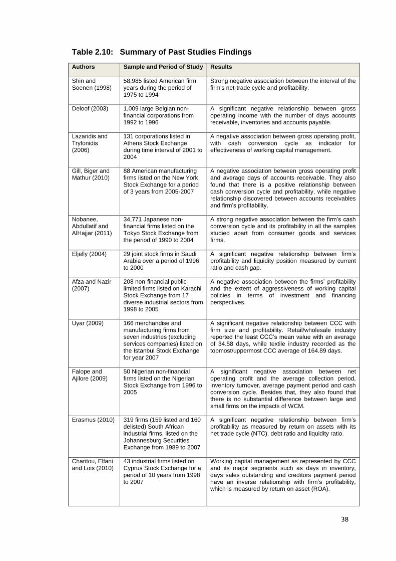
2.10 Summary of Past Studies Findings

The summary of the past studies findings is indicated as per Table 2.10

below.

38

Table 2.10: Summary of Past Studies Findings

Authors Sample and Period of Study Results

Shin and Soenen (1998)

58,985 listed American firm years during the period of 1975 to 1994

Strong negative association between the interval of the firm's net-trade cycle and profitability.

Deloof (2003) 1,009 large Belgian non-financial corporations from 1992 to 1996

A significant negative relationship between gross operating income with the number of days accounts receivable, inventories and accounts payable.

Lazaridis and Tryfonidis (2006)

131 corporations listed in Athens Stock Exchange during time interval of 2001 to 2004

A negative association between gross operating profit, with cash conversion cycle as indicator for effectiveness of working capital management.

Gill, Biger and Mathur (2010)

88 American manufacturing firms listed on the New York Stock Exchange for a period of 3 years from 2005-2007

A negative association between gross operating profit and average days of accounts receivable. They also found that there is a positive relationship between cash conversion cycle and profitability, while negative relationship discovered between accounts receivables and firm’s profitability.

Nobanee, Abdullatif and AlHajjar (2011)

34,771 Japanese non-financial firms listed on the Tokyo Stock Exchange from the period of 1990 to 2004

A strong negative association between the firm’s cash conversion cycle and its profitability in all the samples studied apart from consumer goods and services firms.

Eljelly (2004) 29 joint stock firms in Saudi Arabia over a period of 1996 to 2000

A significant negative relationship between firm’s profitability and liquidity position measured by current ratio and cash gap.

Afza and Nazir (2007)

208 non-financial public limited firms listed on Karachi Stock Exchange from 17 diverse industrial sectors from 1998 to 2005

A negative association between the firms’ profitability and the extent of aggressiveness of working capital policies in terms of investment and financing perspectives.

Uyar (2009)

166 merchandise and manufacturing firms from seven industries (excluding services companies) listed on the Istanbul Stock Exchange for year 2007

A significant negative relationship between CCC with firm size and profitability. Retail/wholesale industry reported the least CCC’s mean value with an average of 34.58 days, while textile industry recorded as the topmost/uppermost CCC average of 164.89 days.

Falope and Ajilore (2009)

50 Nigerian non-financial firms listed on the Nigerian Stock Exchange from 1996 to 2005

A significant negative association between net operating profit and the average collection period, inventory turnover, average payment period and cash conversion cycle. Besides that, they also found that there is no substantial difference between large and small firms on the impacts of WCM.

Erasmus (2010) 319 firms (159 listed and 160 delisted) South African industrial firms, listed on the Johannesburg Securities Exchange from 1989 to 2007

A significant negative relationship between firm’s profitability as measured by return on assets with its net trade cycle (NTC), debt ratio and liquidity ratio.

Charitou, Elfani and Lois (2010)

43 industrial firms listed on Cyprus Stock Exchange for a period of 10 years from 1998 to 2007

Working capital management as represented by CCC and its major segments such as days in inventory, days sales outstanding and creditors payment period have an inverse relationship with firm’s profitability, which is measured by return on asset (ROA).

39

Karaduman, Akbas, Caliskan and Durer (2011)

127 listed corporations in the Istanbul Stock Exchange from year 2005 to 2009

They found that profitability (ROA) can be improved by reducing CCC.

Charitou, Lois and Halim (2012)

718 firms listed on the Indonesia stock exchange for 13 year period, 1998-2010.

CCC and net trade cycle (NTC) have positive relationship with the firm’s profitability, while debt ratio measuring firm’s riskiness was found to have negative relationship with firm’s profitability, which is determined by Return on Assets (ROA).

Zariyawati, Annuar and Abdul Rahim (2009)

1628 firms from six distinct economic segments listed in Bursa Malaysia during year 1996 to 2006.

A strong negative significant association between cash conversion cycle and profit achieved by the firms. Thus, based on their finding, firms are able to accomplish higher profitability by shortening their cash conversion phase.

Nor Edi and Noriza (2010)

172 listed firms in Main Board of Bursa Malaysia from year 2003 to 2007.

A significant negative relationships between working capital segment such as cash conversion cycles, current ratio, current asset to total asset ratio, current liabilities to total asset ratio and debt to asset ratio with firm’s performance in terms of firm’s value that is measured by Tobin Q and profitability measured via return on asset and return on invested capital.

Nasruddin (2006)

145 SME involved in manufacturing sector in Malaysia, from the period of 1999 to 2003

A moderate positive relationship between liquidity and profitability, which implied that profitable firms have higher liquidity positions.

40

CHAPTER 3 : RESEARCH METHODOLOGY

3.0 Introduction

This chapter discusses on the research methodology adopted in the study,

which include review of the research design, research framework, type and

source of data selected, sampling technique, data collection, application of

data analysis techniques to analyze the data obtained and formulation of the

research hypotheses.

3.1 Research Design

The research design for this study is based on secondary data collected from

firms listed in the Main Market of Bursa Malaysia under trading/services and

industrial products sectors from year 2006 to 2010. In this study, the focus is

on services and manufacturing sectors, which are represented by

trading/services and industrial products sector respectively as both the

sectors contributed 85.3% share of Malaysia’s GDP in 2010. The time frame

of five years data is selected for this study from year 2006 to 2010, which is in

conjunction to the emphasis placed by Malaysia’s government via Ninth

Malaysia Plan and Third Industrial Master Plan (IMP3).

In addition, this research is analyzed using panel data regression, which is a

combination of cross-sectional and time-series analysis, in order to make

comparison and determination of the effects of WCM towards firms’

profitability in the services and manufacturing sectors in Malaysia.

41

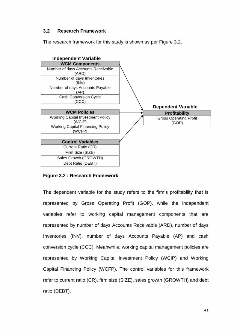
3.2 Research Framework

The research framework for this study is shown as per Figure 3.2.

Independent Variable

WCM Components

Number of days Accounts Receivable (ARD)

Number of days Inventories (INV)

Number of days Accounts Payable (AP)

Cash Conversion Cycle (CCC)

Dependent Variable WCM Policies

Working Capital Investment Policy (WCIP)

Working Capital Financing Policy (WCFP)

Control Variables

Current Ratio (CR)

Firm Size (SIZE)

Sales Growth (GROWTH)

Debt Ratio (DEBT)

Figure 3.2 : Research Framework

The dependent variable for the study refers to the firm’s profitability that is

represented by Gross Operating Profit (GOP), while the independent

variables refer to working capital management components that are

represented by number of days Accounts Receivable (ARD), number of days

Inventories (INV), number of days Accounts Payable (AP) and cash

conversion cycle (CCC). Meanwhile, working capital management policies are

represented by Working Capital Investment Policy (WCIP) and Working

Capital Financing Policy (WCFP). The control variables for this framework

refer to current ratio (CR), firm size (SIZE), sales growth (GROWTH) and debt

ratio (DEBT).

Profitability

Gross Operating Profit (GOP)

42

The variables are then analyzed to determine if there is any significant

relationship between the dependent and independent variables through

Pearson Correlation matrix with the purpose of identification of

multicollinearity. Thus, upon addressing the multicollinearity, there are five

regression models established in order to determine the effect of the WCM

components and WCM policy on the firm’s profitability for a sample of 75 firms

under trading/services and 143 industrial products firms listed in the Main

Market of Bursa Malaysia over a period of five years from year 2006 to 2010.

3.3 Selection of Measures

In this study, there are two types of variables measured; dependent and

independent variable, which the details are as follows:-

3.3.1 Dependent Variable : Gross Operating Profit (GOP)

Deloof (2003) had defined profitability as gross operating income that is

measured by sales less cash costs of goods sold, and divided by total assets

less financial assets, which financial assets refer to shares in other

corporations that formed as substantial segment of total assets. According to

Deloof (2003), return on assets is not included as profitability measurement in

view that for firm that has mostly financial assets on its balance sheet, there is

less influence of the firm’s operating activity towards the return on assets of

the firm. Hence, financial assets are excluded from total assets in the

computation of gross operating income.

43

Other researchers have also supported and applied gross operating profit as

measurement of profitability, which is computed as sales less cost of goods

sold, divided by total assets less financial assets (Lazaridis and Tryfonidis,

2006; Gill, Biger and Mathur, 2010; Dong and Su, 2010; and Napompech,

2012).

Furthermore, according to Gill, Biger and Mathur (2010), earnings before

interest tax depreciation amortization (EBITDA) or pretax profits or net profit

are not being used as profitability measurement as they are of the view that

financing activity need to be eliminated from operational activity that may have

impacts on firm’s profitability on the whole and this is also to enable

connection formed between the firm’s operational performance with operating

ratio and cash conversion cycle.

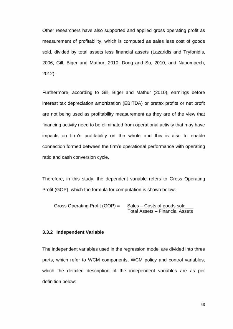
Therefore, in this study, the dependent variable refers to Gross Operating

Profit (GOP), which the formula for computation is shown below:-

Gross Operating Profit (GOP) = Sales – Costs of goods sold___ Total Assets – Financial Assets

3.3.2 Independent Variable

The independent variables used in the regression model are divided into three

parts, which refer to WCM components, WCM policy and control variables,

which the detailed description of the independent variables are as per

definition below:-

44

3.3.2.1 Working Capital Management (WCM) Components

Generally, WCM components consist of number of days account receivables

(ARD), number of days of inventories (INV), number of days accounts payable

(AP) and cash conversion cycle (CCC) as part of inclusive measurement of

WCM. Thus, in order to investigate the effect of WCM towards the profitability

of a firm in services and manufacturing sectors, WCM measurement such as

ARD, INV, AP and CCC have been applied in the panel data regression

model, which the descriptions of the WCM components are as per discussion

below.

3.3.2.1a Number of days Accounts Receivable (ARD)

Accounts receivable (ARD) generally refers to average number of days it

takes for a corporation to obtain collection of payments from its clients, with

the purpose of managing its debtors by reducing the interval of time between

sales and collection of payment from clients (Falope and Ajilore, 2009).

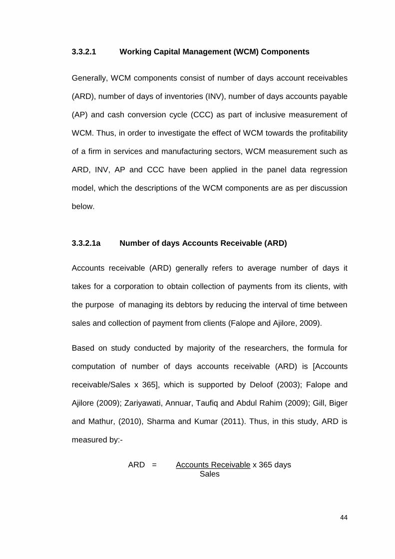
Based on study conducted by majority of the researchers, the formula for

computation of number of days accounts receivable (ARD) is [Accounts

receivable/Sales x 365], which is supported by Deloof (2003); Falope and

Ajilore (2009); Zariyawati, Annuar, Taufiq and Abdul Rahim (2009); Gill, Biger

and Mathur, (2010), Sharma and Kumar (2011). Thus, in this study, ARD is

measured by:-

ARD = Accounts Receivable x 365 days Sales

45

According to Falope and Ajilore (2009), receivables are related to the firm’s

credit collection policy, which also reflects the frequency of conversion of

receivables into cash that is an important part of the WCM. Thus, by granting

trade credit, sales level can be encouraged as it enable ample time for

assessment of products by clients before payment (Long, Malitz and Ravid,

1993; and Deloof and Jegers, 1996). However, by granting liberal credit policy

to clients, although there is an increase in profitability, but liquidity position of

the firm is surrendered (Falope and Ajilore, 2009).

Meanwhile, past literature reviews had reported that there is a significant

negative relationship between profitability and ARD (Deloof, 2003; Lazaridis

and Tryfonidis, 2006; Falope and Ajilore, 2009; Gill, Biger and Mathur, 2010;

Dong and Su, 2010). Furthermore, Deloof (2003) had provided suggestion

that shareholders value can be enhanced further by lessening the number of

days of accounts receivable to an acceptable minimum level, while Lazaridis

and Tryfonidis (2006) indicated that the profitability of the firms can be

improved by lowering the credit interval given to their clients.

3.3.2.1b Number of days Inventories (INV)

Another component of WCM consists of inventories, which is also known as

stock that refers to raw materials, work in progress or finished goods that are

pending manufacturing stage or sales, which the INV is computed as

(Inventories/Purchases) x 365 (Falope and Ajilore, 2009; Sharma and Kumar,

2011). INV also refers to average number of days the stock is kept by the

corporation, which longer INV reflects higher investment in inventory level

46

(Falope and Ajilore, 2009) that is able to minimize the risk of insufficiency of

stock level and lead to greater sales generation (Deloof, 2003). However, on

the other hand, higher investment in INV also infers slow turnover in inventory

which may impact the firm’s profitability.

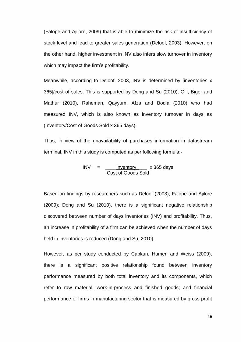
Meanwhile, according to Deloof, 2003, INV is determined by [inventories x

365]/cost of sales. This is supported by Dong and Su (2010); Gill, Biger and

Mathur (2010), Raheman, Qayyum, Afza and Bodla (2010) who had

measured INV, which is also known as inventory turnover in days as

(Inventory/Cost of Goods Sold x 365 days).

Thus, in view of the unavailability of purchases information in datastream

terminal, INV in this study is computed as per following formula:-

INV = ____Inventory ___ x 365 days Cost of Goods Sold

Based on findings by researchers such as Deloof (2003); Falope and Ajilore

(2009); Dong and Su (2010), there is a significant negative relationship

discovered between number of days inventories (INV) and profitability. Thus,

an increase in profitability of a firm can be achieved when the number of days

held in inventories is reduced (Dong and Su, 2010).

However, as per study conducted by Capkun, Hameri and Weiss (2009),

there is a significant positive relationship found between inventory

performance measured by both total inventory and its components, which

refer to raw material, work-in-process and finished goods; and financial

performance of firms in manufacturing sector that is measured by gross profit

47

and earnings before interests and taxes (EBIT). Hence, based on the

researchers finding, there are two possible indications of relationship, either

positive or negative relationship observed between INV and profitability of

firm.

3.3.2.1c Number of days Accounts Payable (AP)

Generally, accounts payable refers to suppliers who had supplied goods or

services that have not been paid by clients, which is also known as amount

owing to creditors that is deemed as free credit and computed as (Accounts

payable/purchases) x 365 (Falope and Ajilore, 2009). This formula is also

supported by Deloof (2003) and Raheman, Qayyum, Afza and Bodla (2010),

which the number of days accounts payable is also known as average

payment period that is assessed as [accounts payable/purchases x 365].

Meanwhile, Lazaridis and Tryfonidis (2006); Dong and Su (2010) and Gill,

Biger and Mathur (2010) have computed AP as (accounts payable/cost of

goods sold) x 365 days.

Thus, in view of as information on purchases is not available as per

datastream terminal, INV in this study is computed as per following formula:-

AP = Accounts Payable_ x 365 days

Cost of Goods Sold

According to past literature reviews, there is a significant negative relationship

established between AP and profitability as reported by Deloof (2003); Falope

and Ajilore (2009), which means that less profitable firms delay payment to

suppliers in order for firms to make evaluation of the feature or quality of

48

products, which are also deemed as an economical and adaptable source of

finance for firms (Deloof, 2003). However, on the other hand, firms incur high

implicit cost via financing granted by suppliers should there be a discount

given by suppliers for prompt payment (Falope and Ajilore, 2009). Thus, the

higher the investment in current assets, the lesser the risk incurred which also

reflects lesser firm’s profitability (Falope and Ajilore, 2009).

Nevertheless, there are also researchers who found a significant positive

association between AP and firms’ profitability, such as Dong and Su (2010),

which means that there is a delay in payment by firms with higher profitability.

Thus, based on the findings by the researchers, there are two possible

indications, either positive or negative relationship found between AP and

profitability of firms.

3.3.2.1d Cash Conversion Cycle (CCC)

Richards and Laughlin (1980) had long established the principle of working

capital management by initiating the idea of CCC as a strong performance

indicator for organizing the firm’s working capital. Short cash conversion cycle

denote that the collection of receivables is prompt and the suppliers being

paid at a slower pace, which reflects improvement on the effectiveness of its

in-house procedures that further translates to greater profitability, greater net

present value of cash flow and greater market valuation of an organization

(Gentry, Vaidyanathan and Lee, 1990). Meanwhile, Besley and Brigham

(2005) define a cash conversion cycle as average period of time taken from

49

acquisition of raw materials being paid to receivables related with sale being

collected.

Cash conversion cycle is deemed as the most dominant and prevalent

measurement for efficiency of working capital management (Gill, Biger and

Mathur, 2010; and Nobanee, Abdullatif and AlHajjar, 2011). In addition, CCC

has also been adopted by other researchers as one of the measurements of

WCM in their study such as Moss and Stine (1993); Eljelly (2004); Lazaridis

and Tryfonidis (2006); Uyar (2009); Zariyawati, Annuar, Taufiq and Abdul

Rahim (2009); Nor Edi Azhar and Noriza (2010); Charitou, Elfani and Lois

(2010); Karaduman, Akbas, Caliskan and Durer (2011); and Charitou, Lois

and Halim (2012).

According to Deloof (2003); Zariyawati, Annuar, Taufiq and Abdul Rahim

(2009); Gill, Biger and Mathur, (2010), for a comprehensive determination of

WCM, CCC is applied that is computed based on [number of days accounts

receivable (ARD) + number of days inventory (INV) – number of days

accounts payable (AP)]. The formula for CCC computation is also supported

by Nobanee, Abdullatif and AlHajjar, (2011), which measured CCC as

[Receivables collection period + Inventory conversion period – Payable

deferral period], meanwhile Raheman, Qayyum and Afza (2011) measured

CCC as [Receivable turnover in days + Inventory turnover in days – Payables

turnover in days).

50

Thus, in this study, CCC is measured by:-

CCC = Number of days Accounts Receivable + Number of days Inventory –

Number of days Accounts Payable

= ARD + INV – AP

A lengthy CCC level may linked to an increase in sales and subsequently

higher profitability gained, but, at the other hand, an extended CCC position

may reflects a lower firms’ profitability in the event the costs of investing in

working capital has escalated beyond the advantages of retaining higher

inventory level and providing higher trade of credit to clients (Akinlo, 2012).

Most of the researchers found a significant negative relationship between

CCC and profitability (Lazaridis and Tryfonidis, 2006; Falope and Ajilore,

2009; Uyar, 2009, Zariyawati, Annuar, Taufiq and Abdul Rahim, 2009; Nor Edi

and Noriza, 2010; Nobanee, Abdullatif and AlHajjar, 2011) which indicates

that profitability can be increased by reducing the CCC level.

However, Deloof (2003) had found an insignificant negative relationship

between CCC and gross operating income under fixed effects estimation

model, in view that gross operating income had decreases with an increase in

number of days accounts receivable, inventories as well as number of days

accounts payable (AP), which have negative relationship with profitability; and

AP had been deducted in computation of CCC. The findings by Deloof (2003)

is also supported by Akinlo (2012), who found an insignificant negative

relationship between CCC and profitability measured by return on assets

(ROA) in fixed effects estimation model, which is due to profitability decreases

51

as a result of an increase in the number of days accounts receivables,

inventories and number of days accounts payable that has been deducted in

CCC calculation.

Meanwhile, Padachi (2006) had found a positive association between CCC

and profitability for Mauritian small manufacturing firms, which the positive

relation is further supported by Gill, Biger and Mathur (2010); Charitou, Lois

and Halim (2012). Thus, based on the researchers’ findings, there is a mixture

of positive and negative relationship observed between CCC and firm’s

profitability.

3.3.2.2 Working Capital Management (WCM) Policy

Working capital management (WCM) plays a vital role as it has impact on the

profitability, risk and value of the firm (Smith, 1980). Thus, there is an

extensive discussion on the tradeoff between risk and return for diverse

working capital policies adopted (Pinches, 1991; Brigham and Ehrhardt, 2004;

Gitman, 2005 and Moyer, McGuigan and Kretlow, 2005). Generally, a firm

opted for aggressive working capital policies enjoyed greater return or

profitability and higher risk level, as compared to a conservative working

capital policies which are linked to lesser risk and profitability (Gardner, Mills

and Pope, 1986; Weinraub and Visscher, 1998).

WCM policy is divided into Working Capital Investment Policy (WCIP) and

Working Capital Financing Policy (WCFP), which the detail of the descriptions

are as discussed below.

52

3.3.2.2a Working Capital Investment Policy (WCIP)

According to Afza and Nazir (2007) and Nazir and Afza (2009), aggressive

investment policy refers to minimum amount being invested in current assets

as compared to fixed assets. Meanwhile, on the other hand, a conservative

investment policy emphasized on higher share of investment in current assets

at the expense of incurring lower profitability (Nazir and Afza, 2009). Thus, an

increase in the firm’s current assets proportionately to total assets reflects a

conservative management style in administering the current assets (Nazir and

Afza, 2009). In contrast, as highlighted by Afza and Nazir (2007) and Nazir

and Afza (2009), lower working capital investment policy (WCIP) ratio in

current assets to its total assets reflects a comparatively aggressive

investment policy.

Furthermore, an extreme concentration in current assets has a negative

impact on the profitability of firm, while a lower current assets position reflects

lower liquidity position and need to deal with the risk of inadequate stock level,

which resulted complexity in sustaining business operations efficiently (Van

Horne and Wachowicz, 2004).

Afza and Nazir (2007) and Nazir and Afza (2009) had computed the extent of

the aggressiveness of working capital investment policy (WCIP) by applying

ratio of aggressive investment policy (AIP) formula as total current assets over

total assets as applied by Weinraub and Visscher (1998). However, in this

study, AIP is also referred to as WCIP, which is represented by the formula

below:-

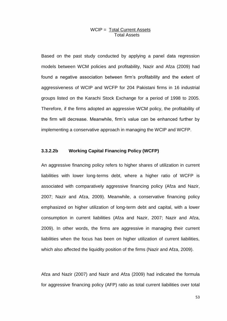
53

WCIP = Total Current Assets Total Assets

Based on the past study conducted by applying a panel data regression

models between WCM policies and profitability, Nazir and Afza (2009) had

found a negative association between firm’s profitability and the extent of

aggressiveness of WCIP and WCFP for 204 Pakistani firms in 16 industrial

groups listed on the Karachi Stock Exchange for a period of 1998 to 2005.

Therefore, if the firms adopted an aggressive WCM policy, the profitability of

the firm will decrease. Meanwhile, firm’s value can be enhanced further by

implementing a conservative approach in managing the WCIP and WCFP.

3.3.2.2b Working Capital Financing Policy (WCFP)

An aggressive financing policy refers to higher shares of utilization in current

liabilities with lower long-terms debt, where a higher ratio of WCFP is

associated with comparatively aggressive financing policy (Afza and Nazir,

2007; Nazir and Afza, 2009). Meanwhile, a conservative financing policy

emphasized on higher utilization of long-term debt and capital, with a lower

consumption in current liabilities (Afza and Nazir, 2007; Nazir and Afza,

2009). In other words, the firms are aggressive in managing their current

liabilities when the focus has been on higher utilization of current liabilities,

which also affected the liquidity position of the firms (Nazir and Afza, 2009).

Afza and Nazir (2007) and Nazir and Afza (2009) had indicated the formula

for aggressive financing policy (AFP) ratio as total current liabilities over total

54

assets. However, in this study, AFP ratio is also referred as WCFP, which is

represented by the formula below :-

WCFP = Total Current Liabilities

Total Assets

3.3.3 Control Variables

The current ratio, firm size, sales growth and debt ratio variables are included

in the regression analysis for control purpose. The control variables are

employed to measure the significance of association between variables and to

determine the extent of the independent variables influence towards the

dependent variables.

3.3.3.1 Current Ratio (CR)

Based on past study conducted by Sharma and Kumar (2011), current ratio

has been included in the model as control variable and is computed as current

assets divided by current liabilities. Other researchers that had also included

current ratio as part of the control variables in the regression model (Charitou,

Lois and Halim, 2012). Current ratio has been included in the model

regression partly due to its role as measuring liquidity position of the firm

traditionally (Zariyawati, Annuar, Taufiq and Abdul Rahim, 2009), as

compared to CCC as a dynamic measurements for liquidity management

(Jose, Lancaster and Stevens, 1996).

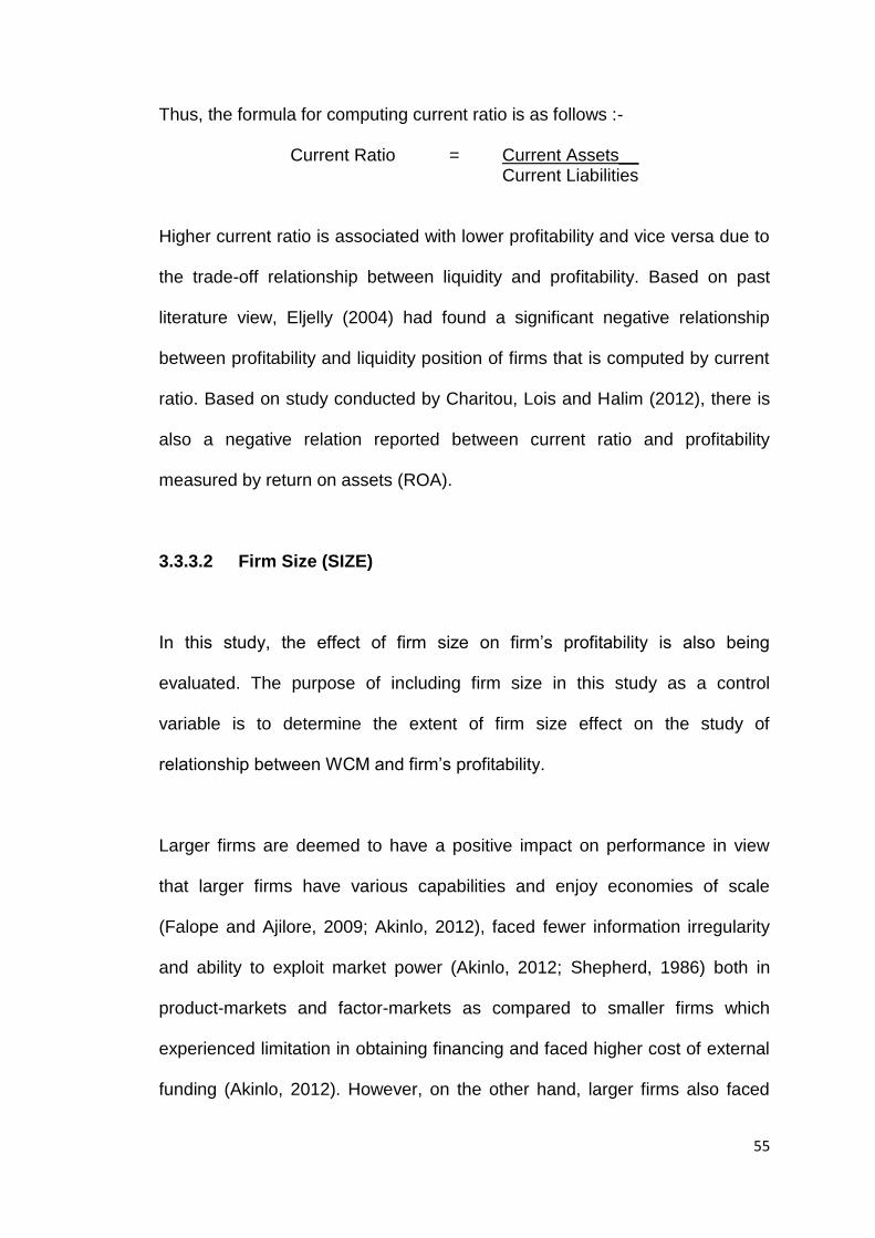
55

Thus, the formula for computing current ratio is as follows :-

Current Ratio = Current Assets__ Current Liabilities

Higher current ratio is associated with lower profitability and vice versa due to

the trade-off relationship between liquidity and profitability. Based on past

literature view, Eljelly (2004) had found a significant negative relationship

between profitability and liquidity position of firms that is computed by current

ratio. Based on study conducted by Charitou, Lois and Halim (2012), there is

also a negative relation reported between current ratio and profitability

measured by return on assets (ROA).

3.3.3.2 Firm Size (SIZE)

In this study, the effect of firm size on firm’s profitability is also being

evaluated. The purpose of including firm size in this study as a control

variable is to determine the extent of firm size effect on the study of

relationship between WCM and firm’s profitability.

Larger firms are deemed to have a positive impact on performance in view

that larger firms have various capabilities and enjoy economies of scale

(Falope and Ajilore, 2009; Akinlo, 2012), faced fewer information irregularity

and ability to exploit market power (Akinlo, 2012; Shepherd, 1986) both in

product-markets and factor-markets as compared to smaller firms which

experienced limitation in obtaining financing and faced higher cost of external

funding (Akinlo, 2012). However, on the other hand, larger firms also faced

56

coordination problems which can negatively influence performance, unlike

smaller firms which are simple to monitor and organized (Falope and Ajilore,

2009).

In the past study, there are several forms of definition being adopted in

measuring firm size. Based on the past study conducted, the most commonly

used measurements for firm size is natural logarithm of sales (Deloof, 2003;

Lazaridis and Tryfonidis, 2006; Gill, Biger and Mathur, 2010; Raheman, Afza,

Qayyum and Bodla, 2010) and natural logarithm of total assets (Falope and

Ajilore, 2009; Nazir and Afza, 2009; Sharma and Kumar, 2011).

In this study, firm size is measured based on natural logarithm of sales, as it is

one of the most commonly used proxies for firm size. Furthermore, according

to Raheman, Afza, Qayyum and Bodla (2010), the natural logarithm of sales

has been applied in computation of size of firms, in view that it is able to

lessen the heteroskedasticity and lower the effect of outliers in the regression

model.

Firm Size = ln (Sales)

Based on past literature review, Deloof (2003); Lazaridis and Tryfonidis, 2006;

Raheman, Afza, Qayyum and Bodla (2010); Akinlo (2012); Charitou, Lois and

Halim (2012) had found a positive relationship between firms size with the

profitability of the firms, which indicates that the larger the size of the firms,

the higher the firms’ profitability in view of the economies of scales enjoyed

that has transformed firms to higher profitability. However, on the other hand,

according to Evanoff and Fortier (1988) and Michael (1985), there is a

57

negative effect of firm size on profitability in view that the positive impact on

firms’ profitability as a result of economies of scale might be partly offset via

diversification of assets by firms, which resulted in a lesser risk and lesser

return as per the portfolio theory. Therefore, based on past literature review,

the expected result on the relationship between firm size and profitability may

be positive or negative relationship.

3.3.3.3 Sales Growth (GROWTH)

One of the control variables that is used in the regression by Zariyawati,

Annuar, Taufiq and Abdul Rahim (2009) is (Sales1 – Sales0)/Sales0 while

Deloof (2003) computed sales growth as [(this year’s sales – previous year’s

sales)/previous year’s sales]. Other researchers which have also included

sales growth as part of the control variables in their studies are Falope and

Ajilore (2009) and Nazir and Afza (2009).

Thus, in this study, sales growth is measured by the following formula:

Sales Growth = Sales1 – Sales0 Sales0

According to Akinlo (2012), sales growth is anticipated to have a positive

relation with profitability in view that higher achievement in sales growth is

derived as a result of better quality of product or services, lesser time required

to evaluate the quality of the products, which leads to lower accounts

receivables days and positive impact on profitability. The positive association

between sales growth and profitability is also supported by other researchers

(Deloof, 2003; Zariyawati, Annuar, Taufiq and Abdul Rahim, 2009; Raheman,

Afza, Qayyum and Bodla, 2010).

58

3.3.3.4 Debt ratio (DEBT)

Deloof (2003) had also used financial debt ratio as control variable, which is

measured by using financial debt divided by total assets, while Gill, Biger and

Mathur (2010) defined financial debt ratio as short-term loans plus long-term

loans divided by total assets. Furthermore, other researchers that have also

included DEBT as control variables had measured debt ratio as total debt

over total assets (Zariyawati, Annuar, Taufiq and Abdul Rahim, 2009; Nor Edi

Azhar, and Noriza, 2010; Sharma and Kumar, 2011). Hence, in this study,

debt ratio is computed using following formula :-

Debt ratio = Total Debt Total Asset

According to Charitou, Lois and Halim (2012); they found a significant

negative relationship between debt ratio and profitability of the firms, as an

increase in debt level raises the interest expense and the possibility of firms

defaulting, which profitability is negatively affected. This finding is supported

by other studies who also found an inverse significant relationship between

debt ratio and profitability (Deloof, 2003; Zariyawati, Annuar, Taufiq and Abdul

Rahim, 2009).

3.4 Summary of proxy variables for WCM Measurements

Table 3.4 shows the summary of the selected working capital management

variables that has impacts on the profitability of firm. The expected sign of the

relationship between the WCM variables and the profitability is also

presented.

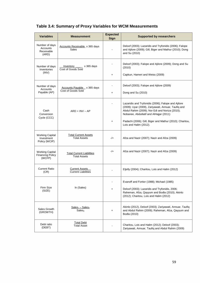
59

Table 3.4: Summary of Proxy Variables for WCM Measurements

Variables Measurement Expected

Sign Supported by researchers

Number of days Accounts

Receivable (ARD)

Accounts Receivable x 365 days Sales

-

Deloof (2003); Lazaridis and Tryfonidis (2006); Falope

and Ajilore (2009); Gill, Biger and Mathur (2010); Dong

and Su (2010)

Number of days Inventories

(INV)

Inventory ___ x 365 days Cost of Goods Sold

-

+

Deloof (2003); Falope and Ajilore (2009); Dong and Su

(2010)

Capkun, Hameri and Weiss (2009)

Number of days Accounts

Payable (AP)

Accounts Payable x 365 days Cost of Goods Sold

-

+

Deloof (2003); Falope and Ajilore (2009)

Dong and Su (2010)

Cash

Conversion

Cycle (CCC)

ARD + INV – AP

-

+

Lazaridis and Tryfonidis (2006); Falope and Ajilore

(2009); Uyar (2009), Zariyawati, Annuar, Taufiq and

Abdul Rahim (2009); Nor Edi and Noriza (2010);

Nobanee, Abdullatif and AlHajjar (2011)

Padachi (2006); Gill, Biger and Mathur (2010); Charitou,

Lois and Halim (2012).

Working Capital

Investment Policy (WCIP)

Total Current Assets Total Assets

-/+ Afza and Nazir (2007); Nazir and Afza (2009)

Working Capital Financing Policy

(WCFP)

Total Current Liabilities Total Assets

-/+

Afza and Nazir (2007); Nazir and Afza (2009)

Current Ratio

(CR)

Current Assets__ Current Liabilities

-

Eljelly (2004); Charitou, Lois and Halim (2012)

Firm Size (SIZE)

ln (Sales)

-

+

Evanoff and Fortier (1988); Michael (1985)

Deloof (2003); Lazaridis and Tryfonidis, 2006;

Raheman, Afza, Qayyum and Bodla (2010); Akinlo

(2012); Charitou, Lois and Halim (2012)

Sales Growth (GROWTH)

Sales1 – Sales0 Sales0

+

Akinlo (2012), Deloof (2003); Zariyawati, Annuar, Taufiq

and Abdul Rahim (2009); Raheman, Afza, Qayyum and

Bodla (2010)

Debt ratio (DEBT)

Total Debt Total Asset

-

Charitou, Lois and Halim (2012); Deloof (2003);

Zariyawati, Annuar, Taufiq and Abdul Rahim (2009)

60

3.5 Development of Hypotheses

Based on the research question and research objectives developed in chapter

1, there are seven hypotheses constructed in this study to investigate on the

three key areas which are (i) the effect of WCM components, (ii) the effect of

WCM policies towards profitability of firms and (iii) the differences between

mean profitability of firms under services and manufacturing sector in

Malaysia during the period of 2006 to 2010.

3.5.1 The Effect of WCM components on Profitability of firms

The hypotheses formed to investigate on the effect of WCM components on

profitability of firms can be summarized based on following four hypotheses

constructed to examine on the effect of number of days Accounts Receivable

(ARD), number of days Inventories (INV), number of days Accounts Payable

(AP) and Cash Conversion Cycle (CCC) towards profitability of firms under

services and manufacturing sector during the period of 2006 to 2010.

The four hypotheses constructed to investigate on the effect of WCM

components on firm’s profitability, which the null and alternative hypotheses

are summarized as follows:-

H1o: There is no significant relationship between Number of days Accounts

Receivable (ARD) and Gross Operating Profit (GOP) of the firms.

H1a: There is a significant relationship between Number of days Accounts

Receivable (ARD) and Gross Operating Profit (GOP) of the firms.

61

H2o : There is no significant relationship between Number of days

Inventories (INV) and Gross Operating Profit (GOP) of the firms.

H2a : There is a significant relationship between Number of days Inventories

(INV) and Gross Operating Profit (GOP) of the firms.

H3o : There is no significant relationship between Number of days Accounts

Payable (AP) and Gross Operating Profit (GOP) of the firms.

H3a : There is a significant relationship between Number of days Accounts

Payable (AP) and Gross Operating Profit (GOP) of the firms.

H4o : There is no significant relationship between Cash Conversion Cycle

(CCC) and Gross Operating Profit (GOP) of the firms.

H4a : There is a significant relationship between Cash Conversion Cycle

(CCC) and Gross Operating Profit (GOP) of the firms.

3.5.2 The Effect of WCM policy on Profitability of firms

The null and alternative hypotheses to investigate on the effect of WCM policy

that are divided into WCIP and WCFP towards the profitability of the firms are

summarized as follows:-

H5o : There is no significant relationship between working capital investment

policy (WCIP) and Gross Operating Profit (GOP) of the firms.

H5a : There is a significant relationship between working capital investment

policy (WCIP) and Gross Operating Profit (GOP) of the firms.

62

H6o : There is no significant relationship between the working capital

financing policy (WCFP) and Gross Operating Profit (GOP) of the firms.

H6a : There is a significant relationship between the working capital financing

policy (WCFP) and Gross Operating Profit (GOP) of the firms.

3.5.3 The differences between mean profitability of firms under

Services and Manufacturing sector in Malaysia

The null and alternative hypotheses to investigate on the differences between

mean profitability of firms under services and manufacturing sector in

Malaysia are summarized as follows:-

H70: There is no significant difference between the mean profitability of

services sector and manufacturing sector.

H7a: There is a significant difference between the mean profitability of

services sector and manufacturing sector.

3.6 Sampling Technique / Design

In this study to investigate on the effect of WCM components and WCM policy

towards the profitability of firms, non-probability sampling technique has been

adopted in view that the selection of the elements in the population as sample

have unknown probability and no pre-arranged opportunity of being selected,

which one of the non-probability designs refers to purposive sampling

(Sekaran and Bougie, 2010). Purposive sampling refers to a non-probability

sample that corresponds to specific criterion stipulated, whereby one of the

63

types is known as judgment sampling (Cooper and Schindler, 2006; Sekaran

and Bougie, 2010).

Therefore, in this study, judgment sampling has been applied due to the

sample is selected based on certain criteria that had been identified as per the

section on data collection method, such as the sample of companies selected

must be continuously listed in the Bursa Malaysia between the periods of

2006 to 2010 and firms with missing data are omitted from the sample of

study. This is further supported by study conducted by Falope and Ajilore

(2009), who had also selected purposive sampling in their study as they had

excluded firms with missing data and newly listed firms when investigating on

the effect of WCM on profitability for a panel of a sample of 50 Nigerian firms

listed on the Nigerian Stock Exchange during 1996 to 2005.

As of 6th October 2012, based on datastream terminal and Bursa Malaysia

website, there are 182 firms listed in the Main Market of Bursa Malaysia under

trading/services sector, meanwhile there are 248 firms listed under industrial

products sector, which represents the population of firms in the services and

manufacturing sectors respectively. Thus, after taken into consideration

removal of firms with missing or incomplete data from the population, the

sample of the study consists of 75 firms listed under trading/services sector,

which represents services sector, while 143 firms listed under industrial

products sector representing manufacturing sector. Data is later analyzed by

using Eview software version 7.0.

64

3.7 Types and Sources of Data

The sample of this study is obtained from secondary data source of firms

listed in the Main Market of Bursa Malaysia under trading/services and

industrial products sectors. The period of study selected is for five years

period, from year 2006 to 2010, which is in tandem Ninth Malaysia Plan,

2006-2010 and the Third Industrial Master Plan (IMP3).

The source for this secondary data is derived from the following sources:-

1. Subscribed datastream terminal 5.1 in University Malaya library

2. The Bursa Malaysia website

3. The Bank Negara Malaysia website

4. The Economic Report of Malaysia website

3.8 Data Collection Method

The sample of firms selected for analysis is based on the following criteria:-

1. The firm is a listed company on the Main Market of Bursa Malaysia

under trading/services or industrial products sectors and has both

complete financial statements and annual reports that allow analysis on

the financial data being conducted during the period of 2006 to 2010.

2. Based on annual report and financial statements of trading/services

and industrial products firms, financial data required are retrieved from

Datastream terminal 5.1, such as annual revenue, accounts receivable

period, inventory turnover period, accounts payable period, current

ratio and debt ratio for the period of 2006 to 2010.

65

3. The shares of the firms are frequently traded in the market which will

reduce the thin trading effect and biasness in the analysis.

4. The sample of companies selected must be continuously listed in the

Main Market of Bursa Malaysia between the period of 2006 to 2010.

Firms with missing data are omitted from the sample of study, which

leaves us with a sample of 75 trading/services firms and 143 industrial

products firms, which represents services and manufacturing sector

respectively.

3.9 Data Analysis Techniques

In this study, panel data regression analysis has been adopted due to it

assumptions that firms are heterogenous, fewer multicolinearity problems

between variables and higher degree of freedom, which resulted in higher

efficiency of the estimator (Baltagi, 2001).

Balanced panel data has been used in this study in view of the characteristic

of data used, which involves both cross sections and time series. According to

Hsiao, Mountain and Ho-Illman (1995), one of the main advantages of using

panel data sets is improvement in the efficiency of econometric estimates, in

view that panel data has higher degrees of freedom and various sample

flexibility than cross-sectional data that may be observed as a panel with T=1,

or time series data with a panel of N=1.

Panel data models are estimated upon determining the correlation between

unobservable heterogeneity ηi of each firm and the explanatory variables,

which the fixed or random effects selection is by applying Hausman (1978)

66

test under null hypothesis E(ηi/Xi,t) = 0 (Falope and Ajilore, 2009). Thus, fixed

effects method is selected as compared to the random effects estimation in

view that based on Hausman test result, as reflected by the Chi-Square

statistic revealed mostly significant at 0.01 levels in all the models. In all the

regression models, the standard errors are computed by applying White’s

correction for heteroscedasticity, as adopted in the study by Deloof (2003)

and Padachi (2006).

Based on the past literature review, there are researchers who had adopted

the panel data methodology in their researches (Deloof, 2003; Falope and

Ajilore, 2009; Zariyawati, Annuar, Taufiq and Abdul Rahim, 2009).

3.10 Panel Data Regression Model

There are five panel data regression models developed in order to test on the

hypotheses developed on the effect of WCM components and WCM policy

towards firm’s profitability measured by GOP. In this study, the regression

models are derived based on model developed by Sharma and Kumar (2011).

However, the model is slightly modified and expanded by incorporating the

effects of WCM policy towards the profitability of firms in services and

manufacturing sectors in Malaysia, by adding in WCIP and WCFP variables in

the model, which are derived as per study carried out by Afza and Nazir

(2007).

The model is further supported by researchers which have analyzed the effect

of individual WCM components separately towards the profitability of firms,

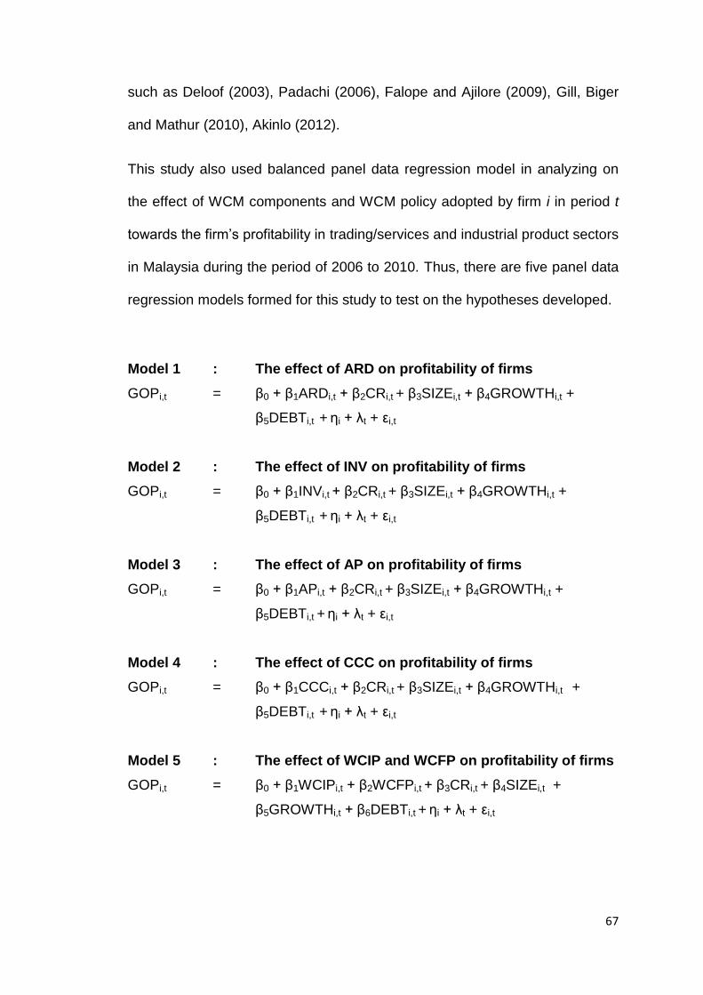
67

such as Deloof (2003), Padachi (2006), Falope and Ajilore (2009), Gill, Biger

and Mathur (2010), Akinlo (2012).

This study also used balanced panel data regression model in analyzing on

the effect of WCM components and WCM policy adopted by firm i in period t

towards the firm’s profitability in trading/services and industrial product sectors

in Malaysia during the period of 2006 to 2010. Thus, there are five panel data

regression models formed for this study to test on the hypotheses developed.

Model 1 : The effect of ARD on profitability of firms

GOPi,t = β0 + β1ARDi,t + β2CRi,t + β3SIZEi,t + β4GROWTHi,t +

β5DEBTi,t + ηi + λt + εi,t

Model 2 : The effect of INV on profitability of firms

GOPi,t = β0 + β1INVi,t + β2CRi,t + β3SIZEi,t + β4GROWTHi,t +

β5DEBTi,t + ηi + λt + εi,t

Model 3 : The effect of AP on profitability of firms

GOPi,t = β0 + β1APi,t + β2CRi,t + β3SIZEi,t + β4GROWTHi,t +

β5DEBTi,t + ηi + λt + εi,t

Model 4 : The effect of CCC on profitability of firms

GOPi,t = β0 + β1CCCi,t + β2CRi,t + β3SIZEi,t + β4GROWTHi,t +

β5DEBTi,t + ηi + λt + εi,t

Model 5 : The effect of WCIP and WCFP on profitability of firms

GOPi,t = β0 + β1WCIPi,t + β2WCFPi,t + β3CRi,t + β4SIZEi,t +

β5GROWTHi,t + β6DEBTi,t + ηi + λt + εi,t

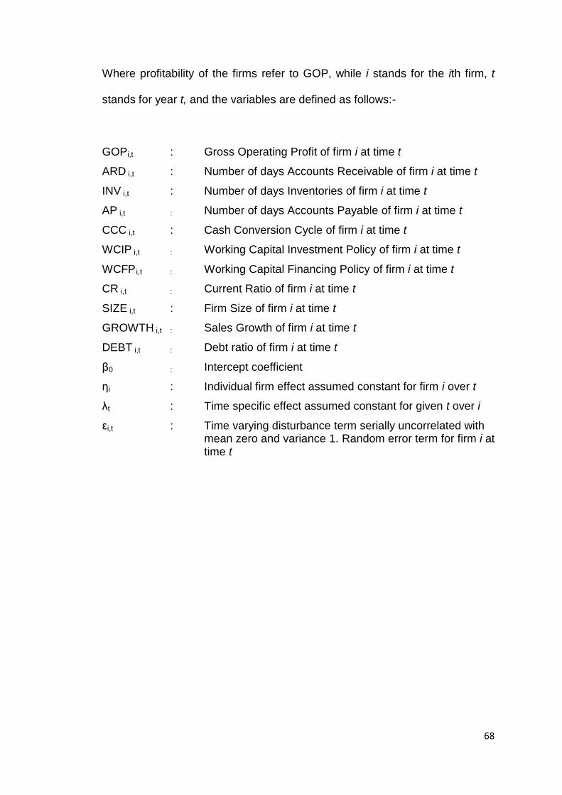
68

Where profitability of the firms refer to GOP, while i stands for the ith firm, t

stands for year t, and the variables are defined as follows:-

GOPi,t : Gross Operating Profit of firm i at time t

ARD i,t : Number of days Accounts Receivable of firm i at time t

INV i,t : Number of days Inventories of firm i at time t

AP i,t : Number of days Accounts Payable of firm i at time t

CCC i,t : Cash Conversion Cycle of firm i at time t

WCIP i,t : Working Capital Investment Policy of firm i at time t

WCFP i,t : Working Capital Financing Policy of firm i at time t

CR i,t : Current Ratio of firm i at time t

SIZE i,t : Firm Size of firm i at time t

GROWTH i,t : Sales Growth of firm i at time t

DEBT i,t : Debt ratio of firm i at time t

β0 : Intercept coefficient

ηi : Individual firm effect assumed constant for firm i over t

λt : Time specific effect assumed constant for given t over i

εi,t : Time varying disturbance term serially uncorrelated with mean zero and variance 1. Random error term for firm i at time t

69

CHAPTER 4 : RESEARCH RESULTS AND ANALYSIS

4.0 Introduction

This chapter discussed on the results obtained from the panel data regression

analysis based on fixed effects estimation. Discussions on the results started

with descriptive statistic, Pearson’s correlation analysis and followed by the

balanced panel data regression analysis using the fixed effects estimation for

the services and manufacturing firms. An analysis of the results obtained with

comparison of the findings gathered from other previous literature review is

also being carried out.

Panel (or longitudinal) data are used in this study as it includes both time-

series and cross-sectional data, which similar variables are observed from

similar cross-sectional sample from various duration of time (Studenmund,

2011). Fixed effects estimation is selected in the analysis in view that one of

the benefits is that it prevents the biasness of variables that has been

excluded which has fixed period of time or also known as “unobserved

heterogeneity or a fixed effect” (Studenmund, 2011).

The data used in this study are obtained from a sample of 75 companies

listed under the Main Market of trading/services sector and a sample of 143

companies listed under the Main Market of industrial products sector for the

period of 2006 to 2010, which represents the services and manufacturing

sector respectively. The analysis of the sample of firms listed under

70

trading/services and industrial products sector are examined by applying the

statistical package of EViews version 7.0.

Subsequently, the effect of WCM components and WCM policies on the

profitability of firms; and the differences in mean profitability of firms in the

services sector and manufacturing sector are investigated by testing on the

hypotheses developed earlier in Chapter 3. There are nine Appendices for

this study as listed in the Appendices section for reference.

4.1 Services Sector

The detailed list of firms under trading/services (services) sector is indicated

as per Appendix 1. There are 75 companies included in the sample of

analysis, out of a total of 182 firms listed under trading/services sector in the

Main Market of Bursa Malaysia as of 6th October 2012, based on datastream

terminal and Bursa Malaysia websites.

4.1.1 Descriptive Statistics

The detailed descriptive statistics for services sector which refers to firms

under trading/services is presented under Appendix 2, whilst the summary of

the key descriptive statistics for the dependent and independent variables are

summarized in Table 4.1.1 below, which presents descriptive statistics for 75

trading/services firms for a period of five years from 2006 to 2010, which has

a total of 375 firm-year observations.

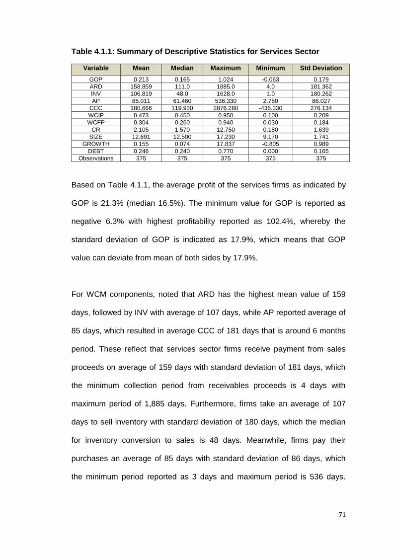
71

Table 4.1.1: Summary of Descriptive Statistics for Services Sector

Variable Mean Median Maximum Minimum Std Deviation

GOP 0.213 0.165 1.024 -0.063 0.179

ARD 158.859 111.0 1885.0 4.0 181.362

INV 106.819 48.0 1628.0 1.0 180.262

AP 85.011 61.460 536.330 2.780 86.027

CCC 180.666 119.930 2876.280 -436.330 276.134

WCIP 0.473 0.450 0.950 0.100 0.209

WCFP 0.304 0.260 0.940 0.030 0.184

CR 2.105 1.570 12.750 0.180 1.639

SIZE 12.691 12.500 17.230 9.170 1.741

GROWTH 0.155 0.074 17.837 -0.805 0.989

DEBT 0.246 0.240 0.770 0.000 0.165

Observations 375 375 375 375 375

Based on Table 4.1.1, the average profit of the services firms as indicated by

GOP is 21.3% (median 16.5%). The minimum value for GOP is reported as

negative 6.3% with highest profitability reported as 102.4%, whereby the

standard deviation of GOP is indicated as 17.9%, which means that GOP

value can deviate from mean of both sides by 17.9%.

For WCM components, noted that ARD has the highest mean value of 159

days, followed by INV with average of 107 days, while AP reported average of

85 days, which resulted in average CCC of 181 days that is around 6 months

period. These reflect that services sector firms receive payment from sales

proceeds on average of 159 days with standard deviation of 181 days, which

the minimum collection period from receivables proceeds is 4 days with

maximum period of 1,885 days. Furthermore, firms take an average of 107

days to sell inventory with standard deviation of 180 days, which the median

for inventory conversion to sales is 48 days. Meanwhile, firms pay their

purchases an average of 85 days with standard deviation of 86 days, which

the minimum period reported as 3 days and maximum period is 536 days.

72

Reportedly, CCC as a measure of efficiency in working capital management

has an average of 181 days with median of 120 days.

In terms of WCM policy, the average value of WCIP is reported as 47.3% of

total assets, while WCFP recorded an average of 30.4% of total assets. The

average current ratio of services firms is reported as 2.1, while the mean size

of the company is 12.7. Meanwhile, the average sales growth and debt ratio

are reported as 15.5% and 24.6% respectively.

4.1.2 Pearson’s Correlation Analysis

Pearson’s Correlation analysis is also being conducted in order to determine

on the relationship between the independent and dependent variables such

as the WCM components, WCM policy and control variables towards the

profitability of the firms that is measured by GOP. Furthermore, based on the

Pearson’s correlation matrix, it also allows detection of any problem of

multicollinearity (Falope and Ajilore, 2009). Multicollinearity can be identified if

there is high (not perfect) correlation between two or more independent

variables (Wooldridge, 2003). The detailed results of Pearson’s correlation

matrix for firms under services sector from year 2006 to 2010 is presented

under Appendix 3 and summarized per Table 4.1.2.

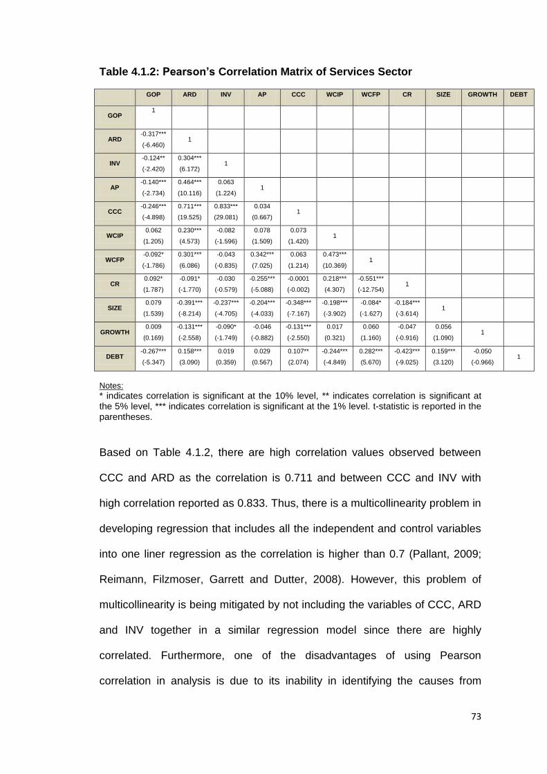
73

Table 4.1.2: Pearson’s Correlation Matrix of Services Sector

GOP ARD INV AP CCC WCIP WCFP CR SIZE GROWTH DEBT

GOP 1

ARD -0.317***

(-6.460) 1

INV -0.124**

(-2.420)

0.304***

(6.172) 1

AP -0.140***

(-2.734)

0.464***

(10.116)

0.063

(1.224) 1

CCC -0.246***

(-4.898)

0.711***

(19.525)

0.833***

(29.081)

0.034

(0.667) 1

WCIP 0.062

(1.205)

0.230***

(4.573)

-0.082

(-1.596)

0.078

(1.509)

0.073

(1.420) 1

WCFP -0.092*

(-1.786)

0.301***

(6.086)

-0.043

(-0.835)

0.342***

(7.025)

0.063

(1.214)

0.473***

(10.369) 1

CR 0.092*

(1.787)

-0.091*

(-1.770)

-0.030

(-0.579)

-0.255***

(-5.088)

-0.0001

(-0.002)

0.218***

(4.307)

-0.551***

(-12.754) 1

SIZE 0.079

(1.539)

-0.391***

(-8.214)

-0.237***

(-4.705)

-0.204***

(-4.033)

-0.348***

(-7.167)

-0.198***

(-3.902)

-0.084*

(-1.627)

-0.184***

(-3.614) 1

GROWTH 0.009

(0.169)

-0.131***

(-2.558)

-0.090*

(-1.749)

-0.046

(-0.882)

-0.131***

(-2.550)

0.017

(0.321)

0.060

(1.160)

-0.047

(-0.916)

0.056

(1.090) 1

DEBT -0.267***

(-5.347)

0.158***

(3.090)

0.019

(0.359)

0.029

(0.567)

0.107**

(2.074)

-0.244***

(-4.849)

0.282***

(5.670)

-0.423***

(-9.025)

0.159***

(3.120)

-0.050

(-0.966) 1

Notes:

* indicates correlation is significant at the 10% level, ** indicates correlation is significant at the 5% level, *** indicates correlation is significant at the 1% level. t-statistic is reported in the parentheses.

Based on Table 4.1.2, there are high correlation values observed between

CCC and ARD as the correlation is 0.711 and between CCC and INV with

high correlation reported as 0.833. Thus, there is a multicollinearity problem in

developing regression that includes all the independent and control variables

into one liner regression as the correlation is higher than 0.7 (Pallant, 2009;

Reimann, Filzmoser, Garrett and Dutter, 2008). However, this problem of

multicollinearity is being mitigated by not including the variables of CCC, ARD

and INV together in a similar regression model since there are highly

correlated. Furthermore, one of the disadvantages of using Pearson

correlation in analysis is due to its inability in identifying the causes from

74

consequences (Deloof, 2003). According to Akinlo (2012), Pearson correlation

also does not offered a consistent indication of the relationship as the

association of each variable with the other independent variables has not

been taken into consideration in the evaluation of the simple bivariate

correlations.

Thus, five panel data regression models have been developed to investigate

on the individual effect of WCM components (ARD, INV, AP, CCC) and WCM

policy (WCIP and WCFP) in services sector, which analysis have been

conducted separately towards the firms’ GOP as dependent variable.

4.1.3 Testing of Hypotheses

Based on the seven hypotheses and five panel data regression models

developed earlier in Chapter 3, the hypotheses are tested by examining on

the effect of WCM components such as ARD, INV, AP, CCC on profitability of

the firms as illustrated as per Model 1, 2, 3 and 4; while the effect of WCM

policy as indicated by WCIP and WCFP on profitability of the firms are

reflected as per Model 5 in Table 4.1.4.

4.1.4 The Effect of Working Capital Management (WCM) components on

Profitability of firms in Services sector

The results of the effect of WCM components on profitability of firms in the

services sector are reflected as per Eview output as per Appendix 4, while the

summary of the panel data regression analysis is presented under Table

4.1.4.

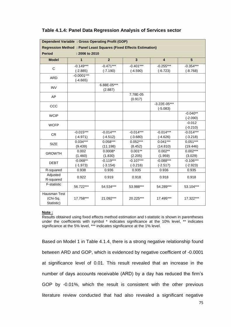
75

Table 4.1.4: Panel Data Regression Analysis of Services sector

Dependent Variable : Gross Operating Profit (GOP)

Regression Method : Panel Least Squares (Fixed Effects Estimation)

Period : 2006 to 2010

Model 1 2 3 4 5

C -0.149***

(-2.885) -0.471***

(-7.190) -0.401***

(-4.590) -0.255***

(-6.723) -0.354***

(-8.768)

ARD -0.0001***

(-4.665)

INV 6.88E-05***

(2.887)

AP 7.78E-05

(0.917)

CCC -3.22E-05***

(-5.083)

WCIP -0.040**

(-2.090)

WCFP -0.012

(-0.210)

CR -0.015***

(-4.971) -0.014***

(-4.512) -0.014***

(-3.680) -0.014***

(-4.626) -0.014***

(-3.218)

SIZE 0.034***

(9.439) 0.058***

(11.198) 0.052***

(8.452) 0.041***

(14.810) 0.051***

(19.446)

GROWTH 0.002

(1.460) 0.0008*

(1.830) 0.001**

(2.205) 0.002**

(1.959) 0.002***

(3.029)

DEBT -0.068**

(-1.973) -0.119***

(-3.154) -0.107***

(-3.216) -0.088***

(-2.517) -0.106***

(-2.923) R-squared 0.938 0.936 0.935 0.936 0.935 Adjusted

R-squared 0.922 0.919 0.918 0.918 0.918

F-statistic

56.722*** 54.534*** 53.988*** 54.289*** 53.104***

Hausman Test

(Chi-Sq.

Statistic)

17.758*** 21.092*** 20.225*** 17.495*** 17.322***

Note : Results obtained using fixed effects method estimation and t-statistic is shown in parentheses under the coefficients with symbol * indicates significance at the 10% level, ** indicates significance at the 5% level, *** indicates significance at the 1% level.

Based on Model 1 in Table 4.1.4, there is a strong negative relationship found

between ARD and GOP, which is evidenced by negative coefficient of -0.0001

at significance level of 0.01. This result revealed that an increase in the

number of days accounts receivable (ARD) by a day has reduced the firm’s

GOP by -0.01%, which the result is consistent with the other previous

literature review conducted that had also revealed a significant negative

76

relationship between profitability and ARD (Deloof, 2003; Lazaridis and

Tryfonidis, 2006; Falope and Ajilore, 2009; Gill, Biger and Mathur, 2010; Dong

and Su, 2010).

Based on the hypotheses developed to examine on the effect of ARD on

GOP:-

H1o: There is no significant relationship between Number of days Accounts

Receivable (ARD) and Gross Operating Profit (GOP) of the firms.

H1a: There is a significant relationship between Number of days Accounts

Receivable (ARD) and Gross Operating Profit (GOP) of the firms.

Thus, based on the result obtained in Model 1 above, the null hypothesis of

H1o is rejected. Therefore, there is a significant negative relationship between

ARD and GOP of firms under services sector, which is consistent with results

obtained by previous researchers.

According to Model 2 in Table 4.1.4, it is revealed that INV has a significant

positive relationship with GOP at 0.01 significant levels or 99% confidence

interval, which indicates that an increase of the number of days inventories

(INV) by a day has increased the GOP of the firms by 0.007%. The result

found is consistent with the study conducted by Capkun, Hameri and Weiss

(2009), which also revealed a significant positive relationship between

inventory performance measured by both total inventory and its components,

which refer to raw material, work-in-process and finished goods; and financial

performance of firms in manufacturing sector that is measured by gross profit

and earnings before interests and taxes (EBIT).

77

Based on the hypotheses developed to examine on the effect of INV on

GOP:-

H2o : There is no significant relationship between Number of days

Inventories (INV) and Gross Operating Profit (GOP) of the firms.

H2a : There is a significant relationship between Number of days Inventories

(INV) and Gross Operating Profit (GOP) of the firms.

Therefore, based on the result obtained in Model 2 above, the null hypothesis

of H2o is rejected. Hence, there is a significant positive relationship between

INV and GOP of firms in services sector during the period of 2006 to 2010.

Based on Model 3 in Table 4.1.4, AP reported an insignificant positive

relationship with GOP, which implies that GOP is increased by 0.008% by

lengthening a day of the accounts payable (AP). Although the result obtained

contradicts with some of the earlier studies that revealed a negative relation

between AP and profitability (Deloof, 2003; Falope and Ajilore, 2009),

however, the result is supported by study conducted by Dong and Su (2010),

who had found a significant positive association between AP and profitability,

which means that there is a delay in payment by firms with higher profitability.

The positive relationship between AP and GOP of the firms may also be due

to firms relied on the trade credit granted by suppliers, which by delaying the

payment has resulted in higher sales by selling the products or services and

thus, achieved higher profitability.

78

Based on the hypotheses developed to examine on the effect of AP on GOP:-

H3o : There is no significant relationship between Number of days Accounts

Payable (AP) and Gross Operating Profit (GOP) of the firms.

H3a : There is a significant relationship between Number of days Accounts

Payable (AP) and Gross Operating Profit (GOP) of the firms.

Thus, based on the result obtained in Model 3 above, the null hypothesis of

H3o is accepted. Therefore, there is a positive relationship but not significant

relationship between AP and GOP of firms under services sector.

Based on Model 4 in Table 4.1.4, CCC has a strong negative relationship with

GOP, which indicates that there is a decrease in GOP by 0.003% by

lengthening the cash conversion cycle (CCC) at 0.01 significant levels. This

means that by reducing the CCC resulted to increase in firm’s profitability.

Furthermore, the inverse relationship found between CCC and GOP is

consistent with the past studies conducted that revealed a highly significant

negative relationship between CCC and GOP, which is supported by Lazaridis

and Tryfonidis (2006); Falope and Ajilore (2009); Uyar (2009), Zariyawati,

Annuar, Taufiq and Abdul Rahim (2009); Nor Edi and Noriza (2010);

Nobanee, Abdullatif and AlHajjar (2011), that indicates that profitability can be

increased by reducing the CCC level.

79

Based on the hypotheses developed to examine on the effect of CCC on

GOP:-

H4o : There is no significant relationship between Cash Conversion Cycle

(CCC) and Gross Operating Profit (GOP) of the firms.

H4a : There is a significant relationship between Cash Conversion Cycle

(CCC) and Gross Operating Profit (GOP) of the firms.

Thus, based on the result obtained in Model 4 above, the null hypothesis of

H4o is rejected. Therefore, there is a significant negative relationship between

CCC and GOP of firms for the services sector during period of 2006 to 2010.

Hence, the firm’s profitability can be increased by reducing the CCC to an

optimum level.

Overall, based on the results derived from Model 1 to Model 4 in Table 4.1.4,

it is suggested that the firm’s finance manager can increase the profitability of

the firm by reducing the ARD and CCC; and increasing the INV level, which

results reveal that ARD, CCC and INV which are part of WCM components

have a significant relationship with profitability of the firms.

4.1.5 The Effect of Working Capital Management (WCM) policies on

Profitability of Firms in Services Sector

Based on Model 5 in Table 4.1.4, the working capital investment policy

(WCIP) of the firms in services sector reveals a statistically negative

relationship with GOP of the firms at 0.05 significant level. This result implies

that there is a positive relationship between WCIP and GOP of the firms,

80

which means that as the WCIP ratio as reflected by total current assets to

total assets decreases, there is an increase in the degree of aggressiveness

of WCIP, which resulted in an increase in the GOP of the firms. Hence, by

adopting an aggressive WCIP, it has resulted in an increase in profitability of

firms in the services sector. The negative coefficient of the WCIP result is

similar to the findings obtained from the study conducted by Hussain, Farooq

and Khan (2012).

Based on the hypotheses developed to examine on the effect of WCIP on

GOP of firms:-

H5o : There is no significant relationship between working capital investment

policy (WCIP) and Gross Operating Profit (GOP) of the firms.

H5a : There is a significant relationship between working capital investment

policy (WCIP) and Gross Operating Profit (GOP) of the firms.

Thus, based on the results reflected in Model 5 in Table 4.1.4, the null

hypothesis of H5o is rejected, in view that there is a significant negative

relationship found between WCIP and GOP of firms in services sector during

period of 2006 to 2010, which reflects an increase in profitability for firms

adopting an aggressive WCIP policy. The negative coefficient of WCIP also

denotes a positive association between the degree of aggressiveness of

investment policy and profitability. The result derived is consistent to the

findings obtained from the study conducted by Hussain, Farooq and Khan

(2012).

81

However, on the other hand, the working capital financing policy of the firms

as represented by WCFP reflects a statistically insignificant negative

relationship with GOP of the firms, which indicates that there is a drop in GOP

by 1.2% by adopting an aggressive WCFP. The negative coefficient of WCFP

also indicates the negative relation between the degree of aggressiveness of

working capital financing policy and profitability. This means that the higher

the WCFP ratio as reflected by total current liabilities to total assets ratio, the

more aggressive the WCFP that resulted in lower GOP for the firms.

Based on the hypotheses developed to examine on the effect of WCFP on

GOP of firms:-

H6o : There is no significant relationship between the working capital

financing policy (WCFP) and Gross Operating Profit (GOP) of the firms.

H6a : There is a significant relationship between the working capital financing

policy (WCFP) and Gross Operating Profit (GOP) of the firms.

Thus, based on the result obtained in Model 5 above, the null hypothesis of

H6o is accepted. Therefore, despite there is a negative relationship between

WCFP and GOP of firms in services sector, which indicates a decrease in the

profitability of the firms, but the effect is not significant for firms adopting an

aggressive policy. The result derived is similar to the findings obtained from

the study conducted by Hussain, Farooq and Khan (2012).

82

4.1.6 The Effect of Control variables on Profitability of Firms

There are four control variables used in the analysis of panel data regression

models, which are CR, SIZE, GROWTH and DEBT. Overall, current ratio (CR)

showed a significant negative relationship at 0.01 level of significant in all the

panel data regression models in Table 4.1.4, which indicates that an increase

in the current ratio as a proxy for liquidity level of the firms resulted in

reduction of firms’ profitability. The result obtained is consistent with the study

on trade-off between liquidity and profitability as highlighted by Eljelly (2004);

Charitou, Lois and Halim (2012).

Meanwhile, other control variable such as SIZE of the firms has reported a

statistically significant positive relationship with GOP at 0.01 significant levels

in all the panel data regression models from Model 1 to Model 5, which the

results are consistent with other previous studies conducted by Deloof (2003);

Lazaridis and Tryfonidis, 2006; Raheman, Afza, Qayyum and Bodla (2010);

Akinlo (2012); Charitou, Lois and Halim (2012). This indicates that the larger

the size of the firms, the higher the profitability achieved as the firms are able

to reap the benefit of economies of scales and obtain easier funding to

expand the business.

The sales growth (GROWTH) of the firms under services sector reported a

positive relationship with significance level of 0.10 in Model 2, 0.05

significance levels in Model 3 and 4; and 0.01 level of significant in Model 5.

The result is consistent with the findings by Akinlo (2012), Deloof (2003);

Zariyawati, Annuar, Taufiq and Abdul Rahim (2009); Raheman, Afza, Qayyum

83

and Bodla (2010) who had found a positive association between GROWTH

and profitability of firms.

The services sector firms had reported a strong inverse relationship between

DEBT and GOP with high significance level at 0.05 in Model 1 and 0.01

significant level in Model 2, 3, 4 and 5, which the results derived are

consistent with other previous literature reviews (Charitou, Lois and Halim,

2012; Deloof, 2003; Zariyawati, Annuar, Taufiq and Abdul Rahim, 2009).

Thus, the significant negative relationship indicates that an increase in debt

level raises the interest expense and the possibility of firms defaulting, which

profitability is negatively affected.

4.1.7 Overall Regression Analysis

Overall, the firms under services sector reported R-squared (R2) that ranges

between 93.5% and 93.8% as reflected in the five panel data regression

models, which indicate that the variation of the GOP has been explained by

the independent variables between 93.5% and 93.8% in the respective

regression models.

Meanwhile, there is a statistically high significant level of F-Statistic that varies

between 53.104 to 56.722 at significance of 0.01 level. This means that the

overall variations in GOP of the firms are explained between 53.10% and

56.72% of the independent variables in the respective regression models.

84

Panel data models are estimated upon determining the correlation between

unobservable heterogeneity ηi of each firm and the explanatory variables,

which the fixed or random effects selection is by applying Hausman (1978)

test under null hypothesis E(ηi/Xi,t) = 0 (Falope and Ajilore, 2009). Thus, fixed

effects method is selected as compared to the random effects estimation in

view that based on Hausman test result, as reflected by the Chi-Square

statistic revealed mostly significant at 0.01 levels in all the models. This

means that null hypothesis E(ηi/Xi,t) = 0 is rejected. Thus, fixed effects model

estimation on panel least square method is selected for the regression.

4.2 Manufacturing Sector

The detailed list of firms under industrial products sector (manufacturing)

sector is indicated as per Appendix 5. There are 143 companies included in

the sample of analysis, out of a total of 248 firms listed under industrial

products sector in Main Market of Bursa Malaysia as of 6th October 2012,

based on datastream terminal and Bursa Malaysia websites.

4.2.1 Descriptive Statistics

The detailed descriptive statistics for manufacturing sector, which also refers

to industrial products sector is presented under Appendix 6, whilst the

summary of the key descriptive statistics for the dependent and independent

variables are summarized in Table 4.2.1 below, which presents descriptive

statistics for 143 industrial products firms for a period of five years from 2006

to 2010, which has a total of 715 firm-year observations.

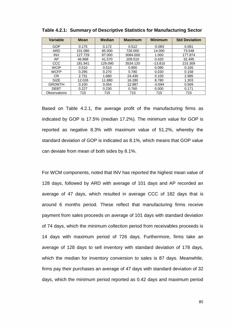
85

Table 4.2.1: Summary of Descriptive Statistics for Manufacturing Sector

Variable Mean Median Maximum Minimum Std Deviation

GOP 0.175 0.172 0.512 -0.083 0.081

ARD 101.080 85.000 726.000 14.000 73.548

INV 127.729 87.000 3084.000 1.000 177.874

AP 46.868 41.570 209.510 0.420 32.495

CCC 181.941 129.090 3534.120 -13.810 215.309

WCIP 0.510 0.510 0.900 0.080 0.165

WCFP 0.295 0.270 0.780 0.030 0.158

CR 2.731 1.680 24.430 0.100 2.985

SIZE 12.026 11.880 16.280 8.780 1.303

GROWTH 0.100 0.054 12.887 -0.694 0.569

DEBT 0.227 0.230 0.760 0.000 0.171

Observations 715 715 715 715 715

Based on Table 4.2.1, the average profit of the manufacturing firms as

indicated by GOP is 17.5% (median 17.2%). The minimum value for GOP is

reported as negative 8.3% with maximum value of 51.2%, whereby the

standard deviation of GOP is indicated as 8.1%, which means that GOP value

can deviate from mean of both sides by 8.1%.

For WCM components, noted that INV has reported the highest mean value of

128 days, followed by ARD with average of 101 days and AP recorded an

average of 47 days, which resulted in average CCC of 182 days that is

around 6 months period. These reflect that manufacturing firms receive

payment from sales proceeds on average of 101 days with standard deviation

of 74 days, which the minimum collection period from receivables proceeds is

14 days with maximum period of 726 days. Furthermore, firms take an

average of 128 days to sell inventory with standard deviation of 178 days,

which the median for inventory conversion to sales is 87 days. Meanwhile,

firms pay their purchases an average of 47 days with standard deviation of 32

days, which the minimum period reported as 0.42 days and maximum period

86

is 209 days. Reportedly, CCC as a measure of efficiency in working capital

management has an average of 182 days with median of 129 days.

In terms of WCM policy, the average value of WCIP is reported as 51% of

total assets, while WCFP recorded an average of 29.5% of total assets. The

average current ratio of manufacturing firms is reported as 2.73, while the

mean size of the firms is 12.03. Meanwhile, the average sales growth and

debt ratio are reported as 10% and 22.7% respectively.

4.2.2 Pearson’s Correlation Analysis

Pearson’s Correlation analysis, which is also known as bivariate correlations

has been performed in order to determine and identify if there is any

significant strong relationship between the independent and dependent

variables such as the WCM components, WCM policy and control variables

towards the profitability of firms measured by GOP under manufacturing

sectors. Furthermore, based on the Pearson’s correlation table, it also allows

detection of any potential of multicollinearity problem (Falope and Ajilore,

2009). The detailed of the overall Pearson’s correlation matrix is shown as per

Appendix 7 and the summary of the Pearson’s correlation matrix is presented

in Table 4.2.2 below.

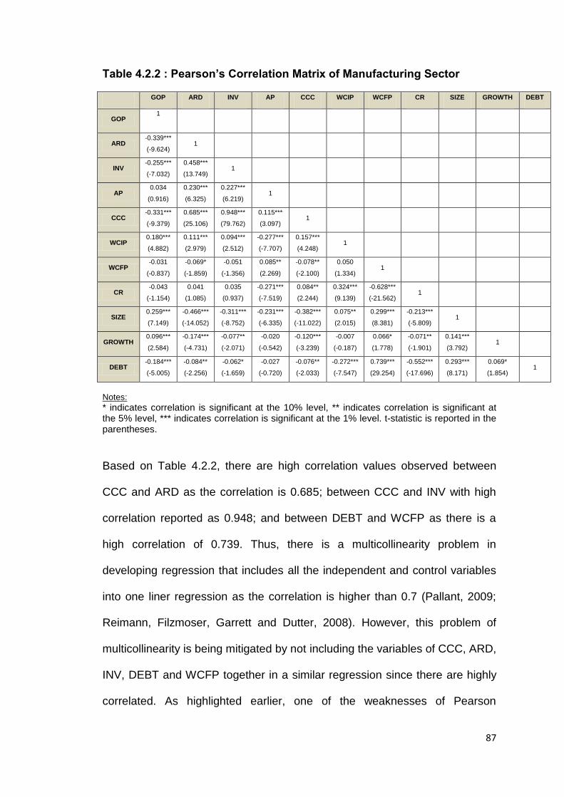
87

Table 4.2.2 : Pearson’s Correlation Matrix of Manufacturing Sector

GOP ARD INV AP CCC WCIP WCFP CR SIZE GROWTH DEBT

GOP 1

ARD -0.339***

(-9.624) 1

INV -0.255***

(-7.032)

0.458***

(13.749) 1

AP 0.034

(0.916)

0.230***

(6.325)

0.227***

(6.219) 1

CCC -0.331***

(-9.379)

0.685***

(25.106)

0.948***

(79.762)

0.115***

(3.097) 1

WCIP 0.180***

(4.882)

0.111***

(2.979)

0.094***

(2.512)

-0.277***

(-7.707)

0.157***

(4.248) 1

WCFP -0.031

(-0.837)

-0.069*

(-1.859)

-0.051

(-1.356)

0.085**

(2.269)

-0.078**

(-2.100)

0.050

(1.334) 1

CR -0.043

(-1.154)

0.041

(1.085)

0.035

(0.937)

-0.271***

(-7.519)

0.084**

(2.244)

0.324***

(9.139)

-0.628***

(-21.562) 1

SIZE 0.259***

(7.149)

-0.466***

(-14.052)

-0.311***

(-8.752)

-0.231***

(-6.335)

-0.382***

(-11.022)

0.075**

(2.015)

0.299***

(8.381)

-0.213***

(-5.809) 1

GROWTH 0.096***

(2.584)

-0.174***

(-4.731)

-0.077**

(-2.071)

-0.020

(-0.542)

-0.120***

(-3.239)

-0.007

(-0.187)

0.066*

(1.778)

-0.071**

(-1.901)

0.141***

(3.792) 1

DEBT -0.184***

(-5.005)

-0.084**

(-2.256)

-0.062*

(-1.659)

-0.027

(-0.720)

-0.076**

(-2.033)

-0.272***

(-7.547)

0.739***

(29.254)

-0.552***

(-17.696)

0.293***

(8.171)

0.069*

(1.854) 1

Notes:

* indicates correlation is significant at the 10% level, ** indicates correlation is significant at the 5% level, *** indicates correlation is significant at the 1% level. t-statistic is reported in the parentheses.

Based on Table 4.2.2, there are high correlation values observed between

CCC and ARD as the correlation is 0.685; between CCC and INV with high

correlation reported as 0.948; and between DEBT and WCFP as there is a

high correlation of 0.739. Thus, there is a multicollinearity problem in

developing regression that includes all the independent and control variables

into one liner regression as the correlation is higher than 0.7 (Pallant, 2009;

Reimann, Filzmoser, Garrett and Dutter, 2008). However, this problem of

multicollinearity is being mitigated by not including the variables of CCC, ARD,

INV, DEBT and WCFP together in a similar regression since there are highly

correlated. As highlighted earlier, one of the weaknesses of Pearson

88

correlation is it does not offered a consistent indication of the relationship as

the association of each variable with the other independent variables has not

been taken into consideration in the evaluation of the simple bivariate

correlations (Akinlo, 2012).

Thus, five panel data regression models have been developed to investigate

on the individual effect of WCM components (ARD, INV, AP, CCC) and WCM

policy (WCIP and WCFP) in manufacturing sector, which analysis have been

conducted separately towards the GOP of the firms as dependent variable.

4.2.3 Testing of Hypotheses

Based on the seven hypotheses and five panel data regression models

developed earlier in Chapter 3, the hypotheses are tested by examining on

the effect of WCM components such as ARD, INV, AP, CCC on profitability of

the firms as illustrated as per Model 1, 2, 3 and 4; while the effect of WCM

policy as indicated by WCIP and WCFP on profitability of the manufacturing

firms are reflected as per Model 5 in Table 4.2.4.

4.2.4 The Effect of Working Capital Management (WCM) components on

Profitability of firms in Manufacturing sector

The results of the effect of WCM components on profitability of firms in

manufacturing sector are reflected as per Eview output as per Appendix 8,

while the panel data regression analysis is summarized as per Table 4.2.4.

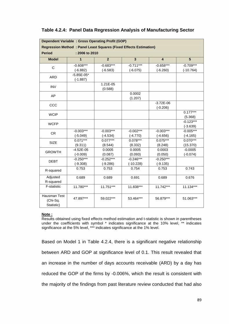
89

Table 4.2.4: Panel Data Regression Analysis of Manufacturing Sector

Dependent Variable : Gross Operating Profit (GOP)

Regression Method : Panel Least Squares (Fixed Effects Estimation)

Period : 2006 to 2010

Model 1 2 3 4 5

C -0.608***

(-6.882) -0.683***

(-6.583)

-0.711***

(-6.075)

-0.658***

(-6.260)

-0.709***

(-10.764)

ARD -5.85E-05*

(-1.887)

INV 1.21E-05

(0.588)

AP 0.0002

(1.207)

CCC -3.72E-06

(-0.206)

WCIP 0.177***

(5.368)

WCFP -0.123***

(-3.639)

CR -0.003***

(-5.049)

-0.003***

(-4.534)

-0.002***

(-4.770)

-0.003***

(-4.656)

-0.005***

(-4.165)

SIZE 0.071***

(9.311)

0.077***

(8.544)

0.078***

(8.332)

0.075***

(8.248)

0.070***

(15.370)

GROWTH -4.52E-05

(-0.009)

0.0005

(0.087)

0.0005

(0.093)

0.0003

(0.050)

-0.0005

(-0.074)

DEBT -0.250***

(-9.308)

-0.252***

(-9.286)

-0.246***

(-10.228)

-0.250***

(-9.135)

R-squared 0.753 0.753 0.754 0.753 0.743

Adjusted

R-squared

0.689 0.689 0.691 0.689 0.676

F-statistic

11.780*** 11.751*** 11.838*** 11.742*** 11.134***

Hausman Test

(Chi-Sq.

Statistic)

47.897*** 59.022*** 53.464*** 56.879*** 51.063***

Note : Results obtained using fixed effects method estimation and t-statistic is shown in parentheses under the coefficients with symbol * indicates significance at the 10% level, ** indicates significance at the 5% level, *** indicates significance at the 1% level.

Based on Model 1 in Table 4.2.4, there is a significant negative relationship

between ARD and GOP at significance level of 0.1. This result revealed that

an increase in the number of days accounts receivable (ARD) by a day has

reduced the GOP of the firms by -0.006%, which the result is consistent with

the majority of the findings from past literature review conducted that had also

90

revealed a significant negative relationship between profitability and ARD

(Deloof, 2003; Lazaridis and Tryfonidis, 2006; Falope and Ajilore, 2009; Gill,

Biger and Mathur, 2010; Dong and Su, 2010).

Based on the hypotheses developed to examine on the effect of ARD on

GOP:-

H1o: There is no significant relationship between Number of days Accounts

Receivable (ARD) and Gross Operating Profit (GOP) of the firms.

H1a: There is a significant relationship between Number of days Accounts

Receivable (ARD) and Gross Operating Profit (GOP) of the firms.

Thus, based on the result obtained in Model 1 above, the null hypothesis of

H1o is rejected. Therefore, there is a significant negative relationship between

ARD and GOP of firms under manufacturing sector, which is consistent with

the results obtained by previous researchers.

Based on Model 2 in Table 4.2.4 that analyze on the effect of INV towards the

firms’ GOP, it is revealed that INV has a positive relationship with GOP, but

the relationship is not significant. This indicates that an increase of the

number of days inventories (INV) by a day has increases the GOP of the firms

by 0.001%, but the result is not significant. The result obtained is found to be

contrary with previous literature review, which mostly revealed a negative

relationship (Deloof, 2003; Falope and Ajilore, 2009; Dong and Su, 2010).

However, the result found is consistent with the study conducted by Capkun,

Hameri and Weiss (2009), which revealed a significant positive relationship

between inventory performance measured by both total inventory and its

91

components, which refer to raw material, work-in-process and finished goods;

and financial performance of firms in manufacturing sector that is measured

by gross profit and earnings before interests and taxes (EBIT).

Based on the hypotheses developed to examine on the effect of INV on

GOP:-

H2o : There is no significant relationship between Number of days

Inventories (INV) and Gross Operating Profit (GOP) of the firms.

H2a : There is a significant relationship between Number of days Inventories

(INV) and Gross Operating Profit (GOP) of the firms.

Therefore, based on the result obtained in Model 2 above, the null hypothesis

of H2o is accepted in view that the positive relation between INV and GOP of

the firms in manufacturing sector is not significant during the period of 2006 to

2010. In Malaysia, one of the reasons an increase in INV will increase the

firm’s profitability is due to the effect of inflation rates in Malaysia which has

been on increasing trend from 0.6% in year 2009 to 1.7% in 2010 (Economic

Report). Hence, firms need to keep a high number of stocks which comprise

of raw materials and finished goods, in anticipation of the price increase that

will affect their bottom line and also in order to be competitive in the industry.

In Model 3 of Table 4.2.4, AP reported an insignificant positive relationship

with GOP, which implies that GOP has increased by 0.02% by lengthening a

day of the accounts payable (AP). Although the result obtained contradicts

with some of the earlier studies that revealed a negative relation between AP

92

and profitability (Deloof, 2003; Falope and Ajilore, 2009), however, the result

is supported by study conducted by Dong and Su (2010), who had found a

significant positive association between AP and profitability, which means that

there is a delay in payment by firms with higher profitability. Furthermore, the

increase in AP may increase the firm’s profitability partly due to well

established firms are given longer trade credit terms by their suppliers due to

their long business relationship and most of their purchases are in bulk

orders.

Based on the hypotheses developed to examine on the effect of AP on GOP:-

H3o : There is no significant relationship between Number of days Accounts

Payable (AP) and Gross Operating Profit (GOP) of the firms.

H3a : There is a significant relationship between Number of days Accounts

Payable (AP) and Gross Operating Profit (GOP) of the firms.

Thus, based on the result obtained in Model 3 above, the null hypothesis of

H3o is accepted due to despite that there is a positive relationship, however,

the relationship is not significant between AP and GOP of the firms under

manufacturing sector.

Based on Model 4 in Table 4.2.4, CCC reported a negative relationship with

GOP, which indicates that there is a decrease in GOP by 0.0004% by

lengthening the cash conversion cycle (CCC). However, the relationship is

found as not significant, which the findings obtained is consistent with the

results derived by Deloof (2003) and Akinlo (2012), who had found an

insignificant negative relationship between CCC and profitability under fixed

93

effects estimation model, in view that profitability decreases as a result of an

increase in the number of days accounts receivable, inventories as well as

number of days accounts payable (AP) that have negative relationship with

profitability; and AP had been deducted in computation of CCC.

Based on the hypotheses developed to examine on the effect of CCC on

GOP:-

H4o : There is no significant relationship between Cash Conversion Cycle

(CCC) and Gross Operating Profit (GOP) of the firms.

H4a : There is a significant relationship between Cash Conversion Cycle

(CCC) and Gross Operating Profit (GOP) of the firms.

Thus, based on the result obtained in Model 4 above, the null hypothesis of

H4o is accepted as there is no significant relationship observed between CCC

and GOP of the manufacturing firms during the period of 2006 to 2010.

Overall, based on the results derived from Model 1 to Model 4 in Table 4.2.4,

it is suggested that the firm’s finance manager can increase the profitability of

the firm in manufacturing sector by reducing the ARD, that represent part of

the WCM components that reveals a significant negative relationship with

profitability of the firms, which is measured by GOP.

94

4.2.5 The Effect of Working Capital Management (WCM) policies on

Profitability of Firms in Manufacturing Sector

Based on Model 5 in Table 4.2.4, the working capital investment policy

(WCIP) of the firms in manufacturing sector reveals a statistically strong

positive relationship with GOP at 0.01 significance level.

Based on the hypotheses developed to examine on the effect of WCIP on

GOP of firms:-

H5o : There is no significant relationship between working capital investment

policy (WCIP) and Gross Operating Profit (GOP) of the firms.

H5a : There is a significant relationship between working capital investment

policy (WCIP) and Gross Operating Profit (GOP) of the firms.

Thus, based on the results reflected in Model 5 in Table 4.2.4, the null

hypothesis of H5o is rejected, in view that there is a significant positive

relationship found between WCIP and GOP of firms in manufacturing sector

during period of 2006 to 2010, which also reflects that profitability can be

increased by adopting a conservative WCIP policy. The positive coefficient of

WCIP ratio also denotes a negative association between the degree of

aggressiveness of investment policy and profitability. This means that when

WCIP as reflected by total current assets to total assets ratio increases, there

is a decrease in the degree of aggressiveness, which resulted in an increase

of GOP of the firms. The result obtained is similar to the finding derived by

Nazir and Afza (2009), who found that there is a negative relationship

95

between the degree of aggressiveness of working capital management

policies and profitability measurement.

However, on the other hand, the firms’ working capital financing policy as

represented by WCFP reflects a statistically significant negative relationship

with GOP, which indicates that there is a drop in GOP by 12.3% by adopting

an aggressive WCFP. The negative coefficient of WCFP also indicates the

negative relation between the degree of aggressiveness of working capital

financing policy (WCFP) and profitability of firms that is measured by gross

operating profit (GOP). This means that the higher the WCFP ratio as

reflected by total current liabilities to total assets ratio, the more aggressive

the WCFP that resulted in lower GOP for the firms. The result obtained is

consistent to the finding derived by Nazir and Afza (2009).

Based on the hypotheses developed to examine on the effect of WCFP on

GOP of firms:-

H6o : There is no significant relationship between the working capital

financing policy (WCFP) and Gross Operating Profit (GOP) of the firms.

H6a : There is a significant relationship between the working capital financing

policy (WCFP) and Gross Operating Profit (GOP) of the firms.

Thus, based on the result obtained in Model 5 in Table 4.2.4, the null

hypothesis of H6o is rejected. Therefore, the manufacturing firms adopting an

aggressive WCFP resulted in a decrease in GOP for firms in manufacturing

96

sector during the implementation of the Ninth Malaysia Plan and Third

Industrial Master Plan (IMP3) from the period of 2006 to 2010.

4.2.6 The Effect of Control variables on Profitability of Firms

There are four control variables used in the analysis of panel data regression

models, which are CR, SIZE, GROWTH and DEBT. Overall, current ratio (CR)

showed a significant negative relationship with GOP at 0.01 level of significant

in all the panel data regression models in Table 4.2.4, which indicates that an

increase in the current ratio as a proxy for liquidity level of the firms resulted in

reduction of firms’ profitability. The result obtained is consistent with the study

on trade-off between liquidity and profitability as highlighted by Eljelly (2004);

Charitou, Lois and Halim (2012).

Meanwhile, other control variable such as SIZE of the firms has reported a

statistically high significant positive relationship with GOP at 0.01 significant

levels in all the panel data regression models from Model 1 to Model 5, which

the results are consistent with other previous studies conducted by Deloof

(2003); Lazaridis and Tryfonidis, 2006; Raheman, Afza, Qayyum and Bodla

(2010); Akinlo (2012); Charitou, Lois and Halim (2012). This indicates that the

larger the size of the firms, the higher the profitability achieved as the firms

are able to reap the benefit of economies of scales and obtain easier funding

to expand the business.

The sales growth (GROWTH) of the firms under manufacturing sector

reported a positive relationship with GOP in Model 2, 3 and 4 of the panel

97

data regression models, but it is not a significant relationship. Meanwhile, an

insignificant negative relationship between sales growth and GOP reported in

Model 1 and Model 5, which the findings contradict with the previous literature

review that found a positive association between GROWTH and profitability of

firms (Akinlo, 2012; Deloof, 2003; Zariyawati, Annuar, Taufiq and Abdul

Rahim, 2009; Raheman, Afza, Qayyum and Bodla, 2010).

The manufacturing firms had reported a strong inverse relationship between

DEBT and GOP with high significance level at 0.01 in all the panel data

regression models, which the results derived are consistent with other

previous literature reviews (Charitou, Lois and Halim, 2012; Deloof, 2003;

Zariyawati, Annuar, Taufiq and Abdul Rahim, 2009). Thus, the significant

negative relationship indicates that an increase in debt level raises the interest

expense and the possibility of firms defaulting, which profitability is negatively

affected.

4.2.7 Overall Regression Analysis

Overall, the firms under manufacturing sector reported R-squared (R2) that

ranges between 74.3% and 75.4% as reflected in the five panel data

regression models, which indicate that the variation of the GOP has been

explained by the independent variables between 74.3% and 75.4% in the

respective regression models.

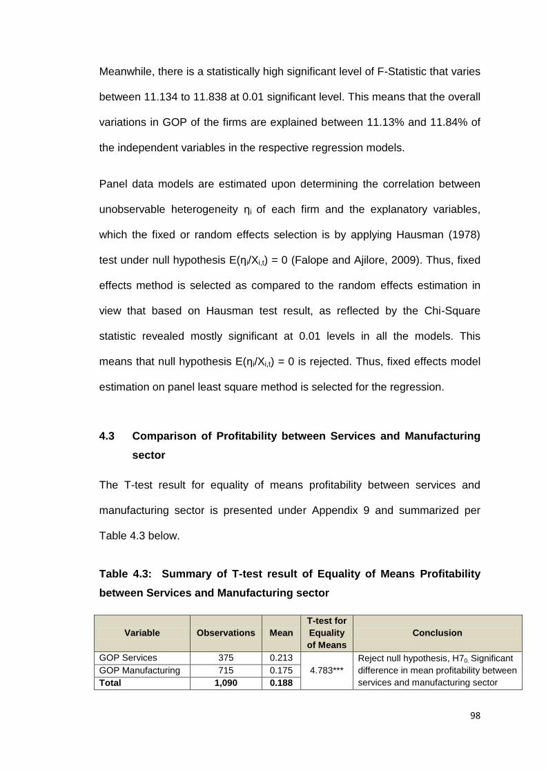
98

Meanwhile, there is a statistically high significant level of F-Statistic that varies

between 11.134 to 11.838 at 0.01 significant level. This means that the overall

variations in GOP of the firms are explained between 11.13% and 11.84% of

the independent variables in the respective regression models.

Panel data models are estimated upon determining the correlation between

unobservable heterogeneity ηi of each firm and the explanatory variables,

which the fixed or random effects selection is by applying Hausman (1978)

test under null hypothesis E(ηi/Xi,t) = 0 (Falope and Ajilore, 2009). Thus, fixed

effects method is selected as compared to the random effects estimation in

view that based on Hausman test result, as reflected by the Chi-Square

statistic revealed mostly significant at 0.01 levels in all the models. This

means that null hypothesis E(ηi/Xi,t) = 0 is rejected. Thus, fixed effects model

estimation on panel least square method is selected for the regression.

4.3 Comparison of Profitability between Services and Manufacturing

sector

The T-test result for equality of means profitability between services and

manufacturing sector is presented under Appendix 9 and summarized per

Table 4.3 below.

Table 4.3: Summary of T-test result of Equality of Means Profitability

between Services and Manufacturing sector

Variable Observations Mean

T-test for

Equality

of Means

Conclusion

GOP Services 375 0.213

4.783***

Reject null hypothesis, H70. Significant

difference in mean profitability between

services and manufacturing sector

GOP Manufacturing 715 0.175

Total 1,090 0.188

99

Based on Table 4.3, it can be concluded that there is a significant difference

in terms of mean of profitability achieved by services sector and

manufacturing sector, as evidenced by the highly significant difference

observed in the t-test for equality of means.

Based on the hypotheses developed to examine on the difference between

the mean profitability of services sector and manufacturing sector:-

H70: There is no significant difference between the mean profitability of

services sector and manufacturing sector.

H7a: There is a significant difference between the mean profitability of

services sector and manufacturing sector.

Hence, based on result in Table 4.3, the null hypothesis of H70 is rejected,

which indicates that there is a significant difference between the mean

profitability of services sector and manufacturing sector during the

implementation of the Ninth Malaysia Plan (9MP) and Third Industrial Master

Plan (IMP3) from period of 2006 to 2010. Furthermore, services sector

reported higher mean value for GOP of 21.3% as compared to mean of GOP

for manufacturing sector of 17.5%.

Thus, this also reflects on the effectiveness of the implementation of the 9MP

and IMP3 policy in promoting services sector and manufacturing sector, which

the result obtained is also in tandem with the Malaysia’s GDP indicators that

revealed a higher share of GDP contribution for services sector of 57.7% as

compared to manufacturing sector share of GDP of 27.6% in 2010.

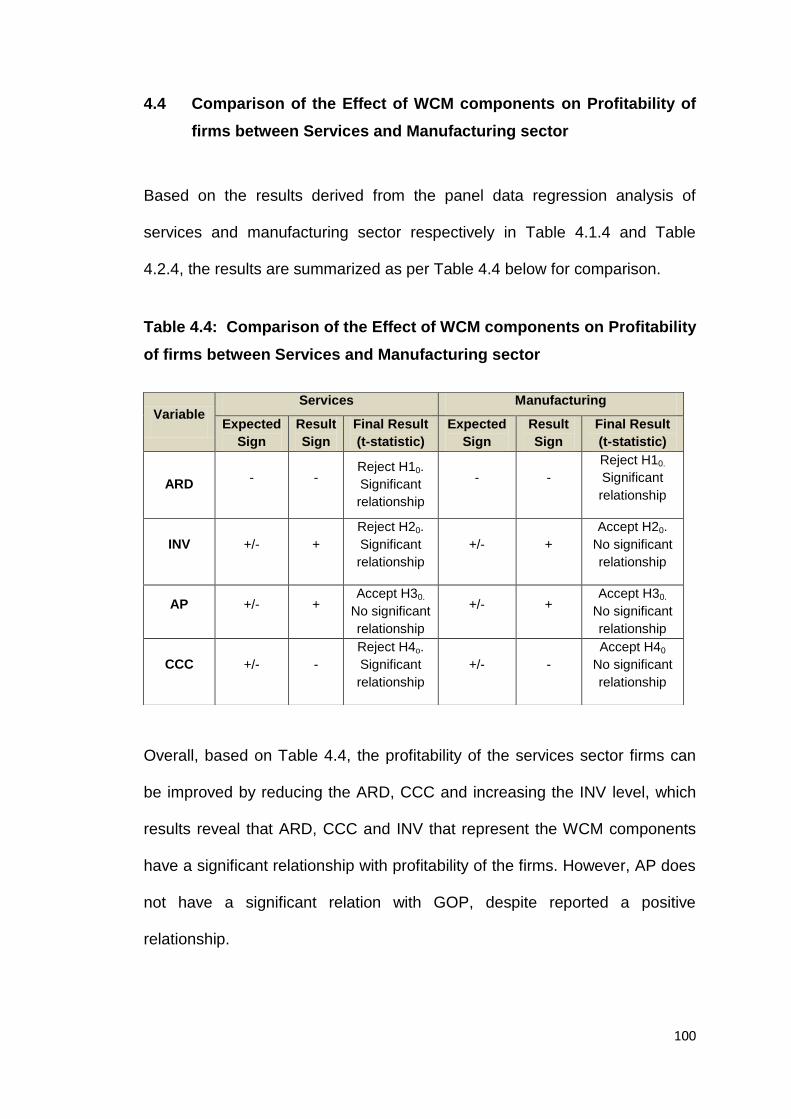
100

4.4 Comparison of the Effect of WCM components on Profitability of

firms between Services and Manufacturing sector

Based on the results derived from the panel data regression analysis of

services and manufacturing sector respectively in Table 4.1.4 and Table

4.2.4, the results are summarized as per Table 4.4 below for comparison.

Table 4.4: Comparison of the Effect of WCM components on Profitability

of firms between Services and Manufacturing sector

Overall, based on Table 4.4, the profitability of the services sector firms can

be improved by reducing the ARD, CCC and increasing the INV level, which

results reveal that ARD, CCC and INV that represent the WCM components

have a significant relationship with profitability of the firms. However, AP does

not have a significant relation with GOP, despite reported a positive

relationship.

Variable Services Manufacturing

Expected

Sign

Result

Sign

Final Result

(t-statistic)

Expected

Sign

Result

Sign

Final Result

(t-statistic)

ARD - -

Reject H10.

Significant

relationship

- -

Reject H10.

Significant

relationship

INV +/- +

Reject H20.

Significant

relationship

+/- +

Accept H20.

No significant

relationship

AP +/- + Accept H30.

No significant

relationship

+/- + Accept H30.

No significant

relationship

CCC +/- -

Reject H4o.

Significant

relationship

+/- -

Accept H40

No significant

relationship

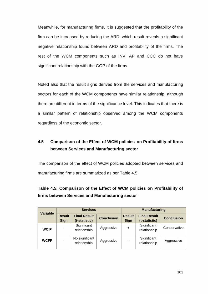
101

Meanwhile, for manufacturing firms, it is suggested that the profitability of the

firm can be increased by reducing the ARD, which result reveals a significant

negative relationship found between ARD and profitability of the firms. The

rest of the WCM components such as INV, AP and CCC do not have

significant relationship with the GOP of the firms.

Noted also that the result signs derived from the services and manufacturing

sectors for each of the WCM components have similar relationship, although

there are different in terms of the significance level. This indicates that there is

a similar pattern of relationship observed among the WCM components

regardless of the economic sector.

4.5 Comparison of the Effect of WCM policies on Profitability of firms

between Services and Manufacturing sector

The comparison of the effect of WCM policies adopted between services and

manufacturing firms are summarized as per Table 4.5.

Table 4.5: Comparison of the Effect of WCM policies on Profitability of

firms between Services and Manufacturing sector

Variable Services Manufacturing

Result

Sign

Final Result

(t-statistic) Conclusion

Result

Sign

Final Result

(t-statistic) Conclusion

WCIP -

Significant

relationship Aggressive +

Significant

relationship Conservative

WCFP - No significant

relationship Aggressive -

Significant

relationship Aggressive

102

Based on Table 4.5, in view that there is a significant negative relationship

reported between WCIP and GOP, it is concluded that the firms in services

sector has been adopting an aggressive WCIP, which had resulted in an

increase in profitability of the firms. Meanwhile, there is no significant

relationship found between WCFP and profitability of firms in the services

sector.

For the manufacturing firms, there is a significant positive relationship

reported between WCIP and GOP during the period of 2006 to 2010, which

also reflects that profitability can be increased by adopting a conservative

WCIP policy. Meanwhile, there is a significant negative relationship found

between WCFP and GOP of the firms, which indicates that there is a

decrease in GOP of the firms by adopting an aggressive WCFP.

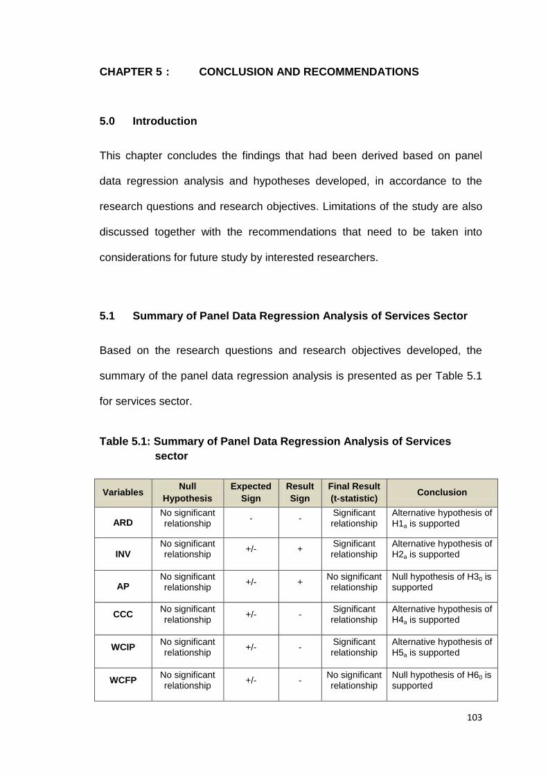
103

CHAPTER 5 : CONCLUSION AND RECOMMENDATIONS

5.0 Introduction

This chapter concludes the findings that had been derived based on panel

data regression analysis and hypotheses developed, in accordance to the

research questions and research objectives. Limitations of the study are also

discussed together with the recommendations that need to be taken into

considerations for future study by interested researchers.

5.1 Summary of Panel Data Regression Analysis of Services Sector

Based on the research questions and research objectives developed, the

summary of the panel data regression analysis is presented as per Table 5.1

for services sector.

Table 5.1: Summary of Panel Data Regression Analysis of Services

sector

Variables Null

Hypothesis

Expected

Sign

Result

Sign

Final Result

(t-statistic) Conclusion

ARD No significant relationship

- - Significant relationship

Alternative hypothesis of H1a is supported

INV No significant relationship

+/-

+

Significant relationship

Alternative hypothesis of H2a is supported

AP No significant relationship

+/- + No significant relationship

Null hypothesis of H30 is supported

CCC No significant relationship

+/- - Significant relationship

Alternative hypothesis of H4a is supported

WCIP No significant relationship

+/- - Significant relationship

Alternative hypothesis of H5a is supported

WCFP No significant relationship

+/- - No significant relationship

Null hypothesis of H60 is supported

104

CR No significant relationship

- -

Significant negative relationship in all the models at 0.01 level of significance

SIZE No significant relationship

+/-

+

Significant positive relationship in all the models at 0.01 level of significance

GROWTH

No significant relationship

+ +

Significant positive relationship at 0.1 level of significant in Model 2, 0.05 level of significant in Model 3 and 4, and 0.01 level of significant in Model 3

DEBT

No significant relationship

-

-

Significant negative relationship found in Model 2 to 5 at 0.01 level of significance, and significant level of 0.05 in Model 1

Overall, based on Table 5.1, the profitability of the firms in services sector can

be improved by reducing the number of days Accounts Receivable (ARD) and

cash conversion cycle (CCC); while increasing the number of days Inventories

(INV) level, which ARD, CCC and INV that represent the WCM components

have a significant relationship with profitability of the firms. However, number

of days Accounts Payable (AP) does not have a significant relationship with

Gross Operating Profit (GOP), despite reported a positive relationship.

Meanwhile, control variable such as current ratio (CR) and debt ratio (DEBT)

reveals a significant negative relationship with profitability, while firm size

(SIZE) and sales growth (GROWTH) reflect a significant positive relationship

with GOP of the services firms.

For services sector, in view that there is a significant negative relationship

reported between working capital investment policy (WCIP) and gross

operating profit (GOP) of the firms, it is concluded that the firms in services

sector has been adopting an aggressive WCIP, which had resulted in an

increase in profitability of the firms. Meanwhile, there is no significant

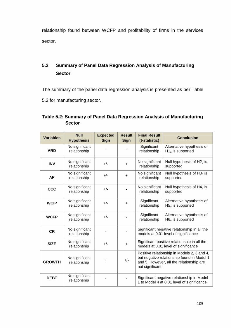
105

relationship found between WCFP and profitability of firms in the services

sector.

5.2 Summary of Panel Data Regression Analysis of Manufacturing

Sector

The summary of the panel data regression analysis is presented as per Table

5.2 for manufacturing sector.

Table 5.2: Summary of Panel Data Regression Analysis of Manufacturing

Sector

Variables Null

Hypothesis

Expected

Sign

Result

Sign

Final Result

(t-statistic) Conclusion

ARD No significant relationship

- - Significant relationship

Alternative hypothesis of H1a is supported

INV No significant relationship

+/- + No significant relationship

Null hypothesis of H20 is supported

AP No significant relationship

+/- + No significant relationship

Null hypothesis of H30 is supported

CCC No significant relationship

+/- - No significant relationship

Null hypothesis of H40 is supported

WCIP No significant relationship

+/- + Significant relationship

Alternative hypothesis of H5a is supported

WCFP No significant relationship

+/- - Significant relationship

Alternative hypothesis of H6a is supported

CR No significant relationship

- - Significant negative relationship in all the models at 0.01 level of significance

SIZE No significant relationship

+/- + Significant positive relationship in all the models at 0.01 level of significance

GROWTH No significant relationship

+ +/-

Positive relationship in Models 2, 3 and 4, but negative relationship found in Model 1 and 5. However, all the relationship are not significant

DEBT No significant relationship

- - Significant negative relationship in Model 1 to Model 4 at 0.01 level of significance

106

For manufacturing firms, it is suggested that the profitability of the firms can

be improved by reducing the number of days Accounts Receivable (ARD),

which reveals a significant negative relationship with profitability of the firms.

The rest of the WCM components such as number of days Inventories (INV),

number of days Accounts Payable (AP) and cash conversion cycle (CCC) do

not have significant relationship with the Gross Operating Profit (GOP) of the

firms. Meanwhile, control variable such as CR and DEBT reveals a significant

negative relationship with profitability, while firms’ SIZE reflects a significant

positive relationship with GOP in the manufacturing firms. However, the sales

growth, GROWTH of the firms revealed a mixture of result between positive

relationship with GOP in Model 2, 3 and 4; but a negative relationship with

GOP in Model 1 and 5. However, the firms’ GROWTH does not have a

significant relationship with GOP in all the models.

There is a significant positive relationship reported between WCIP and GOP

during the period of 2006 to 2010, which also reflects that profitability can be

increased by adopting a conservative WCIP policy. Meanwhile, there is a

significant negative relationship found between WCFP and GOP of the firms,

which indicates that there is a decrease in GOP of the firms by adopting an

aggressive WCFP.

In conclusion, both firms in services and manufacturing sectors indicate that

the profitability of the firms can be enhanced by reducing the number of days

Accounts Receivable (ARD). Hence, the finance managers need to prioritize

in managing its accounts receivable collection regularly by monitoring the

firms’ trade debtors ageing listing promptly. For services sector, besides ARD,

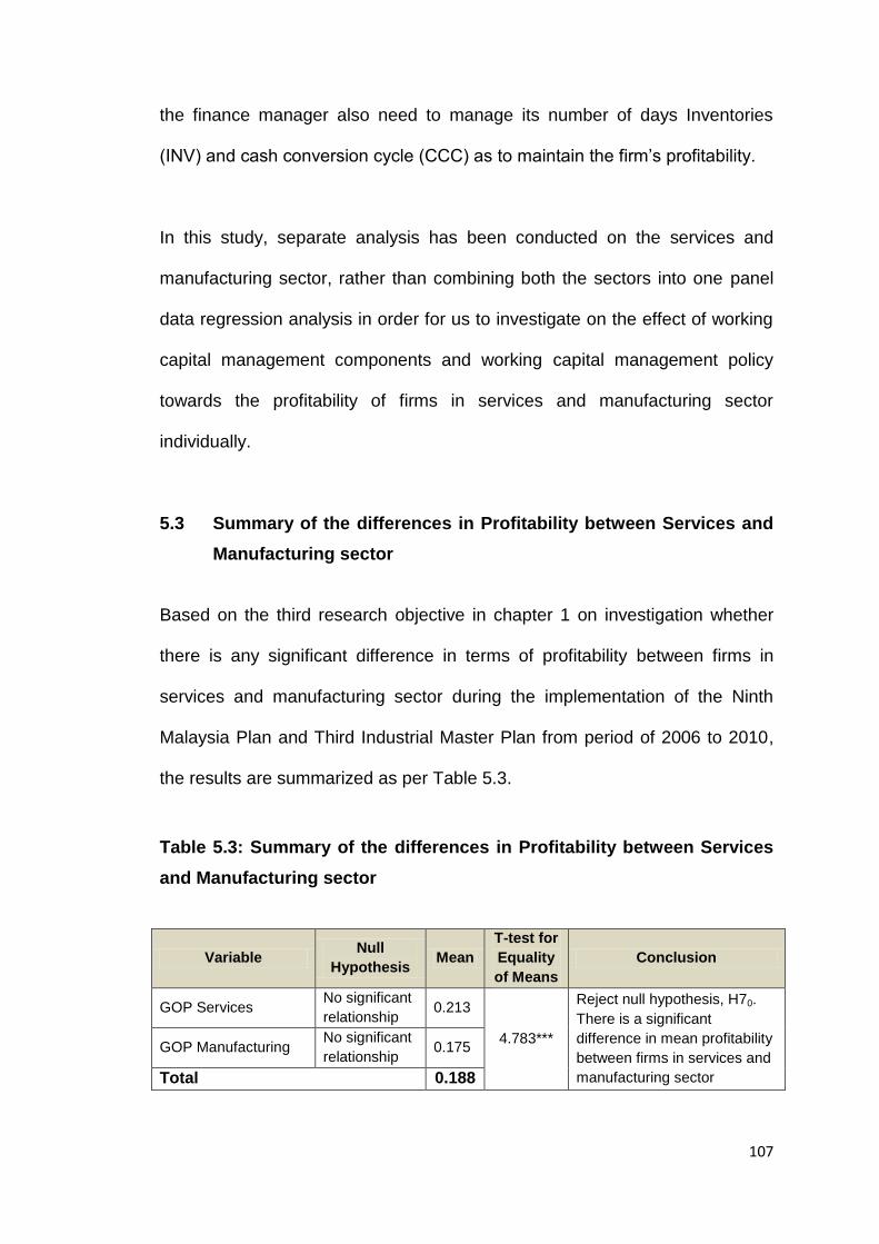
107

the finance manager also need to manage its number of days Inventories

(INV) and cash conversion cycle (CCC) as to maintain the firm’s profitability.

In this study, separate analysis has been conducted on the services and

manufacturing sector, rather than combining both the sectors into one panel

data regression analysis in order for us to investigate on the effect of working

capital management components and working capital management policy

towards the profitability of firms in services and manufacturing sector

individually.

5.3 Summary of the differences in Profitability between Services and

Manufacturing sector

Based on the third research objective in chapter 1 on investigation whether

there is any significant difference in terms of profitability between firms in

services and manufacturing sector during the implementation of the Ninth

Malaysia Plan and Third Industrial Master Plan from period of 2006 to 2010,

the results are summarized as per Table 5.3.

Table 5.3: Summary of the differences in Profitability between Services

and Manufacturing sector

Variable Null

Hypothesis Mean

T-test for

Equality

of Means

Conclusion

GOP Services No significant

relationship 0.213

4.783***

Reject null hypothesis, H70.

There is a significant

difference in mean profitability

between firms in services and

manufacturing sector

GOP Manufacturing No significant

relationship 0.175

Total 0.188

108

Based on Table 5.3, it can be concluded that there is a significant difference

in terms of mean of profitability achieved by firms in services sector and

manufacturing sector, as evidenced by the highly significant difference

observed in the t-test for equality of means of 4.783 at 0.01 significance level.

The result is further supported by higher share of GDP of 57.7% for services

sector as compared to 27.6% share of GDP contributed by manufacturing

sector in year 2010.

5.4 Limitations of the Study

Based on the study carried out in analyzing on the effect of working capital

management (WCM) on profitability of firms in services and manufacturing

sector, there are few limitations observed. One of the limitations is the study

period covers only five years, from year 2006 to 2010, which is deemed as

short duration and hence, unable to ascertain the effectiveness of the WCM

components and WCM policy adopted towards the profitability of firms in the

services sector and manufacturing sector that are represented by

trading/services and industrial products sector respectively during the

implementation of the Ninth Malaysia Plan and Third Industrial Master Plan.

Another limitation observed is the scope of study should be broadened to

include all economic sectors, instead of limiting it to services and

manufacturing sectors, in order to have overall view on the effect of WCM on

profitability of firms in various sectors in Malaysia. Further analysis on the

trading/services and industrial product sectors can be enhanced further by

109

analyzing on the composition of the respective sectors which had contributed

towards the firm’s profitability.

Besides that, profitability measurement such as GOP ratio is calculated based

on book value and there is no measurement of profitability conducted using

current market value. Thus, it does not reflect the current market situation of

the firms in the respective sector for comparison.

Based on the study conducted, there is no external or macroeconomic factor

being taken into consideration such as growth rate of Gross Domestic Product

(GDP) in the regression analysis to investigate on the effect of external or

macroeconomic factor towards the profitability of firms. Furthermore, noted

also that the service sector in this study is represented by trading/services

firms. Hence, the analysis on the effect of working capital management on

profitability of firms in services sector does not represent specifically on the

services sector in view that the trading firms are also formed as part of the

service sector in this study.

5.5 Recommendations for Future Research

Based on the limitations identified, future research should focus and consider

the following recommendations:-

i) The study period can be lengthened by more than five years period in

order for comprehensive analysis and comparison on the effect of

working capital management components and working capital

110

management policy towards profitability of firms in the services and

manufacturing sector.

ii) Future researchers may also be interested to expand their horizon of

study by examining on the effectiveness of the working capital

management (WCM) policy in various economic sectors in Malaysia

and may expand the analysis further to other developing or Asean

countries for comparison on respective working capital management

(WCM) policy.

iii) Profitability measurements can be enhanced to include other

accounting profitability such as Return on Assets and Return on Equity

in the analysis; and can be expanded further to include Tobin’s Q in the

analysis.

iv) Further study may segregates the firms into various firm’s size in order

to determine on the effect of firm’s size towards the firm’s profitability.

v) The analysis of the study can be enhanced further by including

dynamic model in the analysis.

vi) The interested researchers in this study may take into consideration

the macroeconomic factor such as growth rate of Gross Domestic

Product (GDP) to be included in the regression analysis in order to

analyse on the effect of macroeconomic factor towards the profitability

of the firms.

vii) Future research should also separate the trading/services firms, which

was earlier categorised under services sector by analysing purely on

the firms in services sector specifically instead of combining the firms in

111

services with the trading firms in order to investigate on the effect of

working capital management on profitability of firms in services sector.

5.6 Implications of the Study

One of the implications of the study is that it allows finance managers,

management level, practitioner, policy maker and academician to broaden

their knowledge and learning curve on the importance of managing their

working capital efficiently due to its impact towards the firm’s profitability.

Furthermore, by conducting this study, it enables firm minimizing on its cost of

finance and conducts more prudent planning on the working capital

management components such as accounts receivable, inventory and

accounts payable in order to maximize the firm’s profitability and further

enhancement of the shareholders’ wealth. The firm manager may also be able

to determine on the appropriateness of the working capital management

policy selected for their organization and take necessary actions to maximize

on the profitability and shareholders’ wealth of the firms.

In addition, based on the results of this study on the effect of working capital

management components and working capital management policy, it assists

the finance managers in making important decision to achieve optimal

working capital structure for the firms that allows maximization of profit and

shareholders’ wealth.

112

REFERENCES

Afza, T. and Nazir, M.S. (2007), “Is it better to be aggressive or conservative

in managing working capital?”, Journal of Quality and Technology

Management, Vol. 3, No. 2, pp. 11-21.

Akinlo, O.O. (2012), “Effect of working capital on profitability of selected

quoted firms in Nigeria” Global Business Review, Vol. 13, No. 3, pp.

367-381.

Baltagi, B.H. (2001), Econometric Analysis of Panel Data, Second edition,

New York: Wiley.

Bank Negara Malaysia Annual Report from year 2006 to year 2010.

Besley, S. and Brigham, E. (2005), Essentials of Managerial Finance, 13th

Edition, Washington, D.C.: Thomson.

Boer, G. (1999), “Managing the cash gap,” Journal of Accountancy, pp.

27-32.

Brigham, E.F. and Ehrhardt, M.C. (2004), Financial Management: Theory and

Practice, 11th Edition, New York: South-Western College Publishers.

Capkun, V., Hameri, A.P. and Weiss, L.A. (2009), “On the relationship

between inventory and financial performance in manufacturing

companies,” International Journal of Operations & Production

Management, Vol. 29, No. 8, pp. 789-806.

Carpenter, M.D. and Johnson, K.H. (1983), “The association between working

capital policy and operating risk,” The Financial Review, Vol. 18, No. 3,

pp. 106-106.

Charitou, M.S., Elfani, M. and Lois, P. (2010). “The effect of working capital

management on firm’s profitability: Empirical evidence from an

emerging market,” Journal of Business & Economics Research, Vol. 8,

No. 12, pp. 63-68.

Charitou, M, Lois, P. and Halim, B.S. (2012), “The relationship between

working capital management and firm’s profitability: An empirical

investigation for an emerging Asian country,” International Business &

Economics Research Journal, Vol. 11, No. 8, pp. 839-848.

113

Cooper, D.R. and Schindler, P.S. (2006), Business Research Methods, Ninth

Edition, International Edition, New York: McGraw-Hill/Irwin.

Deloof, M. (2003), “Does working capital management affect profitability of

Belgian firms?” Journal of Business Finance & Accounting, Vol. 30,

Nos. 3 & 4, pp. 573-588.

Deloof, M. and Jeger, M. (1996), “Trade Credit, Product Quality and

Intragroup Trade: Some European Evidence,” Financial Management,

Vol. 25, No. 3, pp. 945-968.

Dong, H.P. and Su, J.T. (2010), “The relationship between working capital

management and profitability: A Vietnam case,” International Research

Journal of Finance and Economics, Issue No. 49, pp. 59-67.

Economic Report Malaysia, 2006/2007, 2007/2008, 2008/2009, 2009/2010,

2010/2011 and 2011/2012.

Eljelly, A.M. (2004), “Liquidity-profitability tradeoff: An Empirical Investigation

in an Emerging Market,” International Journal of Commerce and

Management, Vol. 14, No. 2, pp. 48-61.

Erasmus, P.D. (2010), “Working capital management and profitability: The

relationship between the net trade cycle and return on assets,”

Management Dynamics, Vol. 19, No. 1, pp. 2-10.

Evanoff, D.D. and Fortier, D.L. (1988), “Re-evaluation of the structure conduct

performance paradigm in banking,” Journal of Financial Services Res.,

Vol. 1, pp. 277-294.

Falope, O.I. and Ajilore, O.T. (2009), "Working capital management and

corporate profitability: Evidence from panel data analysis of selected

quoted companies in Nigeria," Research Journal of Business

Management, Vol. 3, No. 3, pp. 73-84.

Farris, T. and Hutchison, P. (2002), “Cash-to cash: The new supply chain

management metric”, International Journal of Physical Distribution &

Logistics Management, Vol. 32, No. 4, pp. 288-98.

Filbeck, G. and Krueger, T. (2005), “Industry related differences in working

capital management,” Mid-American Journal of Business, Vol. 20, No.

2, pp. 11-18.

114

Finnerty, J.E. (1993), “Planning cash flow”. American Management

Association.

Fraser, J.A. (1998), “The art of cash management,” Inc., pp. 124-125.

Gardner, M.J., Mills, D.L. and Pope, R.A. (1986), “Working capital policy and

operating risk: An empirical analysis,” Financial Review, Vol. 21, No. 3,

p. 31.

Gentry, J.A., Vaidyanathan, R., Lee, H.W. (1990), “A weighted cash

conversion cycle,” Financial Management, Vol. 19, No. 1, pp. 90-99.

Gill, A., Biger, N. and Mathur, N. (2010), “The Relationship between Working

Capital Management and Profitability: Evidence from the United

States,” Business and Economics Journal, Vol. 2010, pp. 1-9.

Gitman, L.J. (1974), “Estimated corporate liquidity requirements: A simplified

Approach,” The Financial Review, pp. 79-88.

Gitman, L.A. (2005), Principles of Managerial Finance, 11th Edition, New York:

Addison Wesley Publishers.

Hausman, J.A. (1978), Specification tests in econometrics, Econometrica, 46,

pp.1251-1271.

Hill, N.C. and Sartoris, W.L. (1995). Short-Term Financial Management: Text

and Cases, Third Edition, Englewood Cliffs NJ: Prentice-Hall Inc.

Hill, R.C., Griffiths, W., and Lim, G.C. (2008), Principles of Econometrics, 3rd

edition, USA: John Willey & Sons Inc.

Howorth, C. and Westhead, P. (2003), “The focus of working capital

management in UK small firms”, Management Accounting Research,

Vol. 14. No. 2, pp. 94-111.

Hsiao, C., Mountain, D.C. and Ho-Illman, K.F. (1995), “Bayesian integration of

end-use metering and conditional demand analysis,” Journal of

Business and Economic Statistics, No. 13, pp. 315-326.

Hussain, A., Farooq, S.U. and Khan, K.U. (2012), “Aggressiveness and

conservativeness of working capital: A case of Pakistani manufacturing

sector,” European Journal of Scientific Research, Vol. 73, No. 2, pp.

171-182.

115

Jose, M.L., Lancaster, C. and Stevens, J.L., (1996), “Corporate returns and

cash conversion cycles,” Journal of Economics and Finance, Vol. 20,

No. 1, pp. 33-46.

Karaduman, H.A., Akbas, H.E., Caliskan, A.O. and Durer, S. (2011). “The

relationship between working capital management and profitability:

Evidence from an emerging market,” International Research Journal of

Finance and Economics, Issue 62, pp. 61-67.

Lamberson, M. (1995). “Changes in working capital of small firms in relation to

changes in economic activity”, Mid-American Journal of Business, Vol.

10, No. 2, pp. 45-50.

Lancaster, C., Stevens, J. and Jennings, J. (1999), “Corporate liquidity and

the significance of earnings versus cash flow: an examination of

industry effects,” The Journal of Applied Business Research, Vol. 15,

No. 3, pp. 37-46.

Lazaridis, I. and Tryfonidis, D. (2006), “Relationship between working capital

management and profitability of listed companies in the Athens Stock

Exchange,” Journal of Financial Management & Analysis, Vol. 19, No.

1, pp. 26-35.

Leachman, C., Pegels, C.C. and Shin, S.K. (2005), “Manufacturing

performance: evaluation and determinants,” International Journal of

Operations & Production Management, Vol. 25, No.9, pp. 851-874.

Loeser, D. (1988), “Improving accounts receivable management,” Journal of

Accounting, Vol. 166, No. 5, pp. 116-117.

Long, M.S., Malitz, I.B. and Ravid, S.A. (1993), “Trade Credit, Quality

Guarantees and Product Marketability,” Financial Management, Vol.

22, No. 4, pp. 117-127.

McDonald, J.T. (1999), “The Determinants of Firm Profitability in Australian

Manufacturing,” The Economic Record, Vol. 75, No. 229. pp.115-126.

Michael, S., (1985), “Evidence on the (Non) relationship between

concentration and profit ability in banking,” Journal of Credit Banking,

Vol. 17, pp. 69-83.

Moss, J. and Stine, B. (1993), “Cash conversion cycle and firm size: A study

of retail firms,” Managerial Finance, Vol. 19, No. 8, pp. 25-35.

116

Moyer, R.C., McGuigan, J.R. and Kretlow, W.J. (2005), Contemporary

Financial Management, 10th Edition, New York: South-Western College

Publication.

Napompech, K. (2012), “Effects of working capital management on the

profitability of Thai listed firms,” Vol. 3, No. 3, pp. 227- 232.

Nasruddin, Z. (2006), “Liquidity-profitability trade off: Is it evident among

Malaysian SMEs?,” IJMS, Vol. 13, No. 2, pp. 107-118.

Nazir, M.S. and Afza, T. (2009), “Impact of aggressive working capital

management policy on firms’ profitability,” The IUP Journal of Applied

Finance, Vol. 15, No. 8, pp.19-30.

Ninth Malaysia Plan, 2006 – 2010 (2006). The Economic Planning Unit, Prime

Minister's Department, Putrajaya. Retrieved from

http://www.epu.gov.my/html/themes/epu/html/rm9/html/english.htm

(Accessed on 12 August 2012)

Niresh, J.A. (2012), “Trade-off between liquidity & profitability: A study of

selected manufacturing firms in Sri Lanka,” Journal of Arts, Science &

Commerce, Vol. 3, Issue 4 (2), pp. 34-40.

Nobanee, H., Abdullatif, M., AlHajjar, M. (2011), “Cash conversion cycle and

firm’s performance of Japanese firms,” Asian Review of Accounting,

Vol. 19, No. 2, pp. 147-156.

Nor Edi Azhar, M. and Noriza, M.S. (2010), “Working capital management:

The effect of market valuation and profitability in Malaysia,”

International Journal of Business and Management, Vol. 5, No. 11, pp.

140-147.

Padachi, K. (2006), “Trends in working capital management and its Impact on

firms’ performance: An analysis of Mauritian small manufacturing

firms,” International Review of Business Research Papers, Vol. 2, No.

2, pp. 45-58.

Pallant, J.F. (2009), SPSS Survival Manual, 3rd edition, Sydney: Ligare Book

Printer

Pinches, G.E. (1991), Essentials of Financial Management, 4th Edition, New

York: HarperCollins College Division.

117

Raheman, A and Nasr, M. (2007), “Working capital management and

profitability – Case of Pakistani firms,” International Review of Business

Research Papers, Vol. 3, No. 1, pp. 279-300.

Raheman, A., Afza, T., Qayyum, A. and Bodla, M.A. (2010), “Working capital

management and corporate performance of manufacturing sector in

Pakistan,” International Research Journal of Finance and Economics,

Issue 47, pp. 151-163.

Raheman, A., Qayyum, A. and Afza, T. (2011), “Sector-wise performance of

working capital management measures and profitability using ratio

analysis,” Interdisciplinary Journal of Contemporary Research in

Business, Vol. 3, No. 8, pp. 285-310.

Raheman, A., Qayyum, A., Afza, T. and Bodla, M.A. (2010). Sector-wise

analysis of working capital management and firm performance in

manufacturing sector of Pakistan. Interdisciplinary Journal of

Contemporary Research in Business, Vol. 2, No. 7, pp. 412-433.

Reimann, C., Filzmoser, P., Garrett, R. G. and Dutter, R. (2008). Statistical

Data Analysis Explained. Applied Environmental Statistics with R. John

Wiley & Sons Ltd.

Richards, V.D. and Laughlin, E.J. (1980), “A cash conversion cycle approach

to liquidity analysis,” Financial Management, Vol. 9, No. 1, pp. 32-38.

Ross, S.A., Westerfield, R.W. and Jordan, B.D. (2010). Fundamentals of

Corporate Finance, Ninth Edition (Alternate Edition).McGraw-Hill/Irwin.

Ross, S.A., Westerfield, R.W. and Jaffe, J. (2005). Corporate Finance. Fifth

Edition. McGraw Hill Irwin.

Securities Commission Annual Report from year 2006 to year 2010.

Sekaran, U. and Bougie, R. (2010), Research methods for business : A Skill

building approach, Fifth Edition, John Wiley & Sons Ltd.

Sharma, A.K. and Kumar, S. (2011), “Effect of working capital management

on firm profitability: Empirical evidence from India,” Global Business

Review, Vol, 12, No. 1, pp. 159-173.

118

Shepherd, W.G. (1986), On the core concepts of industrial organization. In

W.G. Shepherd and H.W. De Jong (Eds), Mainstreams in industrial

organization. Dordrecht: Martinus Nijhoff Publishers.

Shin, H. and Soenen, L. (1998), “Efficiency of working capital and corporate

Profitability,” Financial Practice and Education, Vol. 8, No.2, pp.37-45.

Smith, K. V. (1980). Profitability versus Liquidity Tradeoffs in Working Capital

Management. In K. V. Smith (Ed.), In Readings on the management of

Working Capital, New York, St. Paul MN: West Publishing Company,

pp. 549-562.

Smith, M.B. and Begemann, E. (1997). Measuring associations between

working capital and return on investment, South African Journal of

Business Management, Vol. 28, No. 1, pp. 1-5.

Studenmund, A.H. (2011), Using econometrics a practical guide, Sixth

Edition, International Edition, Boston: Pearson Education Inc.

Tenth Malaysia Plan, 2011-2015 (2010). The Economic Planning Unit, Prime

Minister’s Department, Putrajaya. Retrieved from

http://www.pmo.gov.my/dokumenattached/RMK/RMK10_Eds.pdf

(Accessed on 12 August 2012)

Third Industrial Master Plan (IMP3). Retrieved from

http://www.miti.gov.my/cms/content.jsp?id=com.tms.cms.section.Sectio

n_8ab58e8f-7f000010-72f772f7-dbf00272 (Accessed on 12 August

2012).

Third Industrial Master Plan (IMP3) 2006 – 2020 (2006). Ministry of

International Trade and Industry, Malaysia. Retrieved from

http://www.miti.gov.my/cms/content.jsp?id=com.tms.cms.article.Article_

8e595aba-7f000010-72f772f7-733da6e4 (Accessed on 12 August

2012).

Uyar, A. (2009), “The relationship of cash conversion cycle with firm size and

profitability: An empirical investigation in Turkey,” International

Research Journal of Finance and Economics, Issue 24, pp. 186-192.

Van Horne, J.C. and Wachowicz, J.M. (2004), Fundamentals of Financial

Management, 12th Edition, New York: Prentice Hall Publishers.

119

Weinraub, H.J. and Visscher, S. (1998), “Industry practice relating to

aggressive conservative working capital policies,” Journal of Financial

and Strategic Decisions, Vol. 11, No. 2, pp. 11-18.

Wooldridge, J.M. (2003), Introductory Econometrics: A modern approach, 2nd

edition, USA: Thomson, South-Western.

Zariyawati, M.A , Taufiq, H., Annuar, M.N. and Sazali, A. (2010),

“Determinants of Working Capital Management: Evidence from

Malaysia,” International Conference on Financial Theory and

Engineering, pp. 190-194.

Zariyawati, M.A., Annuar, M. N., Taufiq, H. and Abdul Rahim, A. S. (2009),

“Working capital management and corporate performance: Case of

Malaysia,” Journal of Modern Accounting and Auditing, Vol.5, No. 11,

pp. 47-54.

Zariyawati, M.A , Annuar, M.N. and Abdul Rahim A.S. (2009), “Effect of

working capital management on profitability of firms in Malaysia,” Paper

presented in International Symposium on Finance and Accounting

(ISFA), 6–8 July, Malaysia. Retrieved from http://bai-conference.org/

BAI2009/Pages/submissions/ isfa2009_submission_13.doc. (accessed

on 21 July 2012).

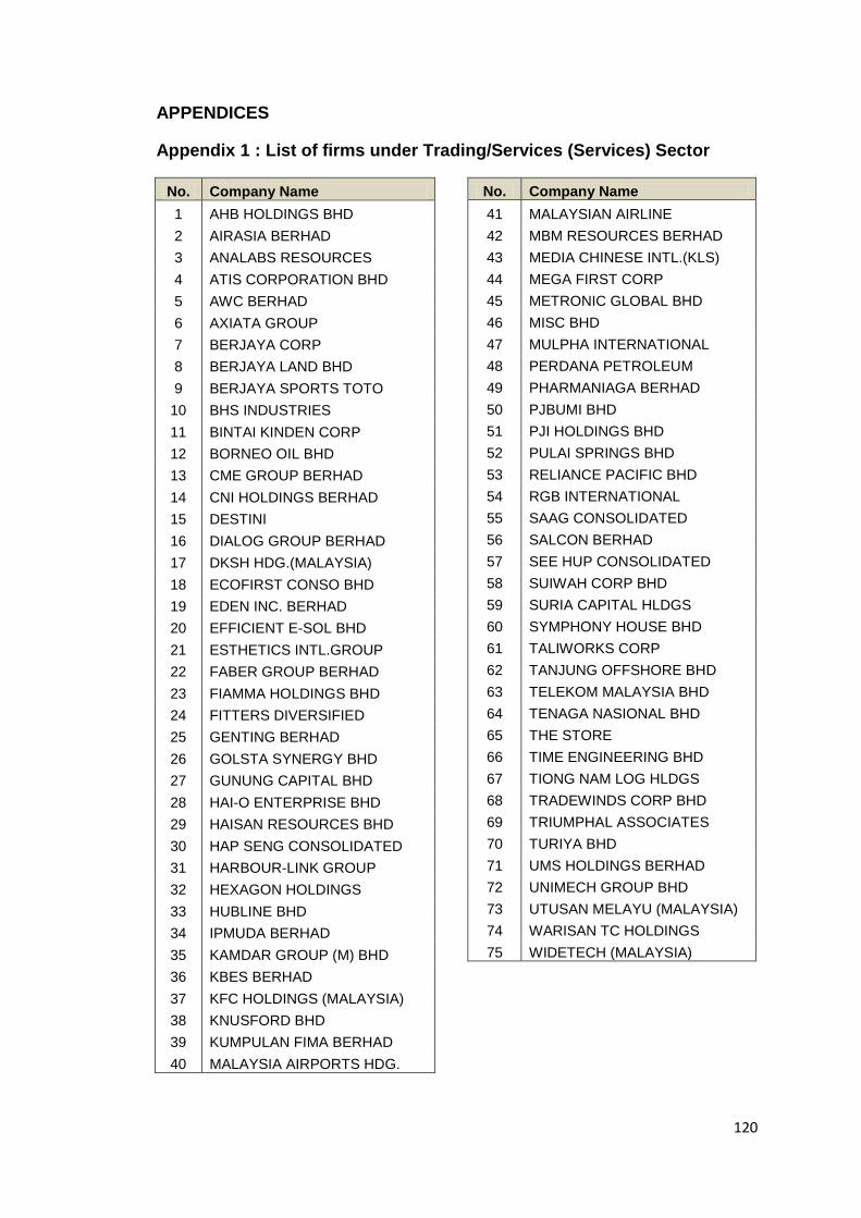
120

APPENDICES

Appendix 1 : List of firms under Trading/Services (Services) Sector

No. Company Name

1 AHB HOLDINGS BHD

2 AIRASIA BERHAD

3 ANALABS RESOURCES

4 ATIS CORPORATION BHD

5 AWC BERHAD

6 AXIATA GROUP

7 BERJAYA CORP

8 BERJAYA LAND BHD

9 BERJAYA SPORTS TOTO

10 BHS INDUSTRIES

11 BINTAI KINDEN CORP

12 BORNEO OIL BHD

13 CME GROUP BERHAD

14 CNI HOLDINGS BERHAD

15 DESTINI

16 DIALOG GROUP BERHAD

17 DKSH HDG.(MALAYSIA)

18 ECOFIRST CONSO BHD

19 EDEN INC. BERHAD

20 EFFICIENT E-SOL BHD

21 ESTHETICS INTL.GROUP

22 FABER GROUP BERHAD

23 FIAMMA HOLDINGS BHD

24 FITTERS DIVERSIFIED

25 GENTING BERHAD

26 GOLSTA SYNERGY BHD

27 GUNUNG CAPITAL BHD

28 HAI-O ENTERPRISE BHD

29 HAISAN RESOURCES BHD

30 HAP SENG CONSOLIDATED

31 HARBOUR-LINK GROUP

32 HEXAGON HOLDINGS

33 HUBLINE BHD

34 IPMUDA BERHAD

35 KAMDAR GROUP (M) BHD

36 KBES BERHAD

37 KFC HOLDINGS (MALAYSIA)

38 KNUSFORD BHD

39 KUMPULAN FIMA BERHAD

40 MALAYSIA AIRPORTS HDG.

No. Company Name

41 MALAYSIAN AIRLINE

42 MBM RESOURCES BERHAD

43 MEDIA CHINESE INTL.(KLS)

44 MEGA FIRST CORP

45 METRONIC GLOBAL BHD

46 MISC BHD

47 MULPHA INTERNATIONAL

48 PERDANA PETROLEUM

49 PHARMANIAGA BERHAD

50 PJBUMI BHD

51 PJI HOLDINGS BHD

52 PULAI SPRINGS BHD

53 RELIANCE PACIFIC BHD

54 RGB INTERNATIONAL

55 SAAG CONSOLIDATED

56 SALCON BERHAD

57 SEE HUP CONSOLIDATED

58 SUIWAH CORP BHD

59 SURIA CAPITAL HLDGS

60 SYMPHONY HOUSE BHD

61 TALIWORKS CORP

62 TANJUNG OFFSHORE BHD

63 TELEKOM MALAYSIA BHD

64 TENAGA NASIONAL BHD

65 THE STORE

66 TIME ENGINEERING BHD

67 TIONG NAM LOG HLDGS

68 TRADEWINDS CORP BHD

69 TRIUMPHAL ASSOCIATES

70 TURIYA BHD

71 UMS HOLDINGS BERHAD

72 UNIMECH GROUP BHD

73 UTUSAN MELAYU (MALAYSIA)

74 WARISAN TC HOLDINGS

75 WIDETECH (MALAYSIA)

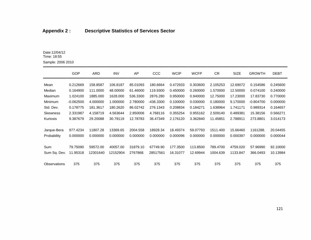
121

Appendix 2 : Descriptive Statistics of Services Sector

Date:12/04/12 Time: 18:55

Sample: 2006 2010 GOP ARD INV AP CCC WCIP WCFP CR SIZE GROWTH DEBT

Mean 0.212669 158.8587 106.8187 85.01093 180.6664 0.472933 0.303600 2.105253 12.69072 0.154586 0.245600

Median 0.164900 111.0000 48.00000 61.46000 119.9300 0.450000 0.260000 1.570000 12.50000 0.074100 0.240000

Maximum 1.024100 1885.000 1628.000 536.3300 2876.280 0.950000 0.940000 12.75000 17.23000 17.83730 0.770000

Minimum -0.062500 4.000000 1.000000 2.780000 -436.3300 0.100000 0.030000 0.180000 9.170000 -0.804700 0.000000

Std. Dev. 0.178775 181.3617 180.2620 86.02742 276.1343 0.208834 0.184271 1.638964 1.741171 0.989314 0.164657

Skewness 2.331987 4.158719 4.563644 2.850006 4.768116 0.355254 0.955162 2.509140 0.489381 15.38156 0.566271

Kurtosis 9.387679 29.20088 30.79119 12.78783 36.47349 2.176120 3.362840 11.45851 2.788911 273.8801 3.014173

Jarque-Bera 977.4234 11807.28 13369.65 2004.558 18928.34 18.49374 59.07793 1511.400 15.66460 1161288. 20.04455

Probability 0.000000 0.000000 0.000000 0.000000 0.000000 0.000096 0.000000 0.000000 0.000397 0.000000 0.000044

Sum 79.75090 59572.00 40057.00 31879.10 67749.90 177.3500 113.8500 789.4700 4759.020 57.96990 92.10000

Sum Sq. Dev. 11.95318 12301640 12152904 2767868. 28517561 16.31077 12.69944 1004.639 1133.847 366.0493 10.13984

Observations 375 375 375 375 375 375 375 375 375 375 375

122

Appendix 3 : Pearson’s Correlation Matrix of Services Sector

Covariance Analysis: Ordinary Date: 12/04/12 Time: 19:35 Sample: 2006 2010 Included observations: 375 Correlation t-Statistic Probability GOP ARD INV AP CCC WCIP WCFP CR SIZE GROWTH DEBT

GOP 1.000000 ----- -----

ARD -0.317197 1.000000 -6.459680 ----- 0.0000 -----

INV -0.124336 0.304401 1.000000 -2.420101 6.171847 ----- 0.0160 0.0000 -----

AP -0.140180 0.464009 0.063239 1.000000 -2.734325 10.11649 1.223797 ----- 0.0065 0.0000 0.2218 -----

CCC -0.245827 0.710944 0.833031 0.034496 1.000000 -4.898001 19.52457 29.08120 0.666631 ----- 0.0000 0.0000 0.0000 0.5054 -----

WCIP 0.062249 0.230428 -0.082341 0.077886 0.073325 1.000000 1.204573 4.573371 -1.595683 1.508809 1.419963 ----- 0.2291 0.0000 0.1114 0.1322 0.1565 -----

WCFP -0.092068 0.300564 -0.043199 0.341835 0.062711 0.473041 1.000000 -1.785719 6.086282 -0.835086 7.025114 1.213537 10.36949 ----- 0.0750 0.0000 0.4042 0.0000 0.2257 0.0000 -----

CR 0.092114 -0.091243 -0.029964 -0.254774 -0.000115 0.217679 -0.551054 1.000000 1.786606 -1.769582 -0.578966 -5.088425 -0.002230 4.307374 -12.75377 ----- 0.0748 0.0776 0.5630 0.0000 0.9982 0.0000 0.0000 -----

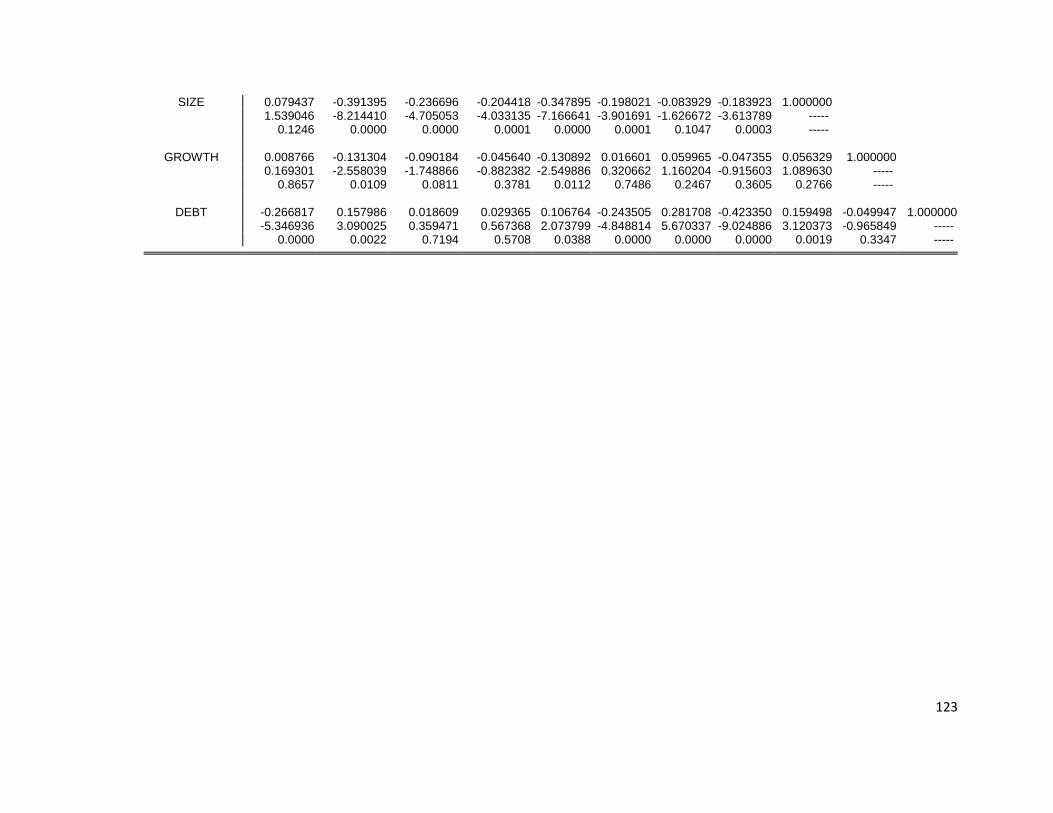
123

SIZE 0.079437 -0.391395 -0.236696 -0.204418 -0.347895 -0.198021 -0.083929 -0.183923 1.000000 1.539046 -8.214410 -4.705053 -4.033135 -7.166641 -3.901691 -1.626672 -3.613789 ----- 0.1246 0.0000 0.0000 0.0001 0.0000 0.0001 0.1047 0.0003 -----

GROWTH 0.008766 -0.131304 -0.090184 -0.045640 -0.130892 0.016601 0.059965 -0.047355 0.056329 1.000000 0.169301 -2.558039 -1.748866 -0.882382 -2.549886 0.320662 1.160204 -0.915603 1.089630 ----- 0.8657 0.0109 0.0811 0.3781 0.0112 0.7486 0.2467 0.3605 0.2766 -----

DEBT -0.266817 0.157986 0.018609 0.029365 0.106764 -0.243505 0.281708 -0.423350 0.159498 -0.049947 1.000000 -5.346936 3.090025 0.359471 0.567368 2.073799 -4.848814 5.670337 -9.024886 3.120373 -0.965849 ----- 0.0000 0.0022 0.7194 0.5708 0.0388 0.0000 0.0000 0.0000 0.0019 0.3347 -----

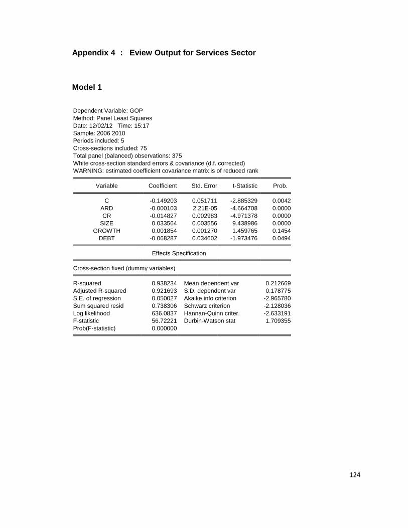
124

Appendix 4 : Eview Output for Services Sector

Model 1

Dependent Variable: GOP

Method: Panel Least Squares

Date: 12/02/12 Time: 15:17

Sample: 2006 2010

Periods included: 5

Cross-sections included: 75

Total panel (balanced) observations: 375

White cross-section standard errors & covariance (d.f. corrected)

WARNING: estimated coefficient covariance matrix is of reduced rank Variable Coefficient Std. Error t-Statistic Prob. C -0.149203 0.051711 -2.885329 0.0042

ARD -0.000103 2.21E-05 -4.664708 0.0000

CR -0.014827 0.002983 -4.971378 0.0000

SIZE 0.033564 0.003556 9.438986 0.0000

GROWTH 0.001854 0.001270 1.459765 0.1454

DEBT -0.068287 0.034602 -1.973476 0.0494 Effects Specification Cross-section fixed (dummy variables) R-squared 0.938234 Mean dependent var 0.212669

Adjusted R-squared 0.921693 S.D. dependent var 0.178775

S.E. of regression 0.050027 Akaike info criterion -2.965780

Sum squared resid 0.738306 Schwarz criterion -2.128036

Log likelihood 636.0837 Hannan-Quinn criter. -2.633191

F-statistic 56.72221 Durbin-Watson stat 1.709355

Prob(F-statistic) 0.000000

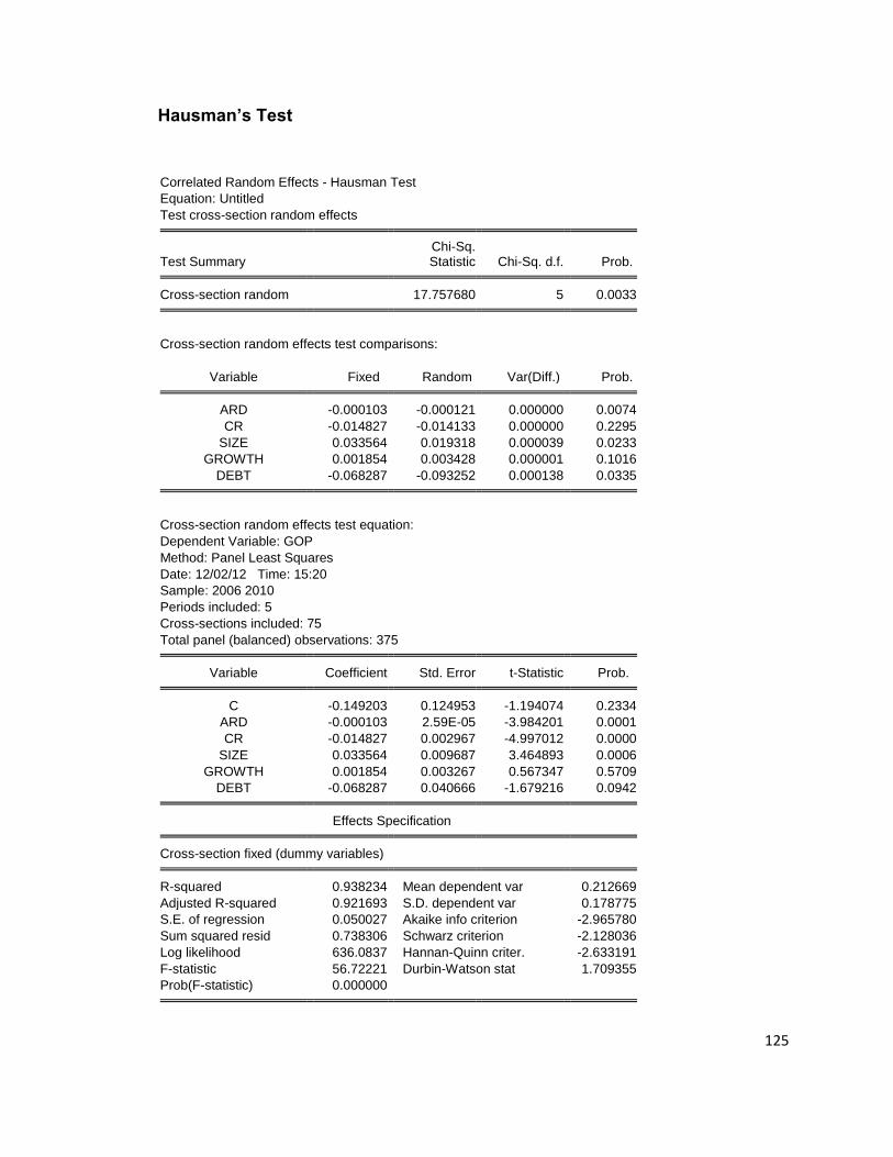
125

Hausman’s Test

Correlated Random Effects - Hausman Test

Equation: Untitled

Test cross-section random effects

Test Summary Chi-Sq. Statistic Chi-Sq. d.f. Prob.

Cross-section random 17.757680 5 0.0033

Cross-section random effects test comparisons:

Variable Fixed Random Var(Diff.) Prob. ARD -0.000103 -0.000121 0.000000 0.0074

CR -0.014827 -0.014133 0.000000 0.2295

SIZE 0.033564 0.019318 0.000039 0.0233

GROWTH 0.001854 0.003428 0.000001 0.1016

DEBT -0.068287 -0.093252 0.000138 0.0335

Cross-section random effects test equation:

Dependent Variable: GOP

Method: Panel Least Squares

Date: 12/02/12 Time: 15:20

Sample: 2006 2010

Periods included: 5

Cross-sections included: 75

Total panel (balanced) observations: 375 Variable Coefficient Std. Error t-Statistic Prob. C -0.149203 0.124953 -1.194074 0.2334

ARD -0.000103 2.59E-05 -3.984201 0.0001

CR -0.014827 0.002967 -4.997012 0.0000

SIZE 0.033564 0.009687 3.464893 0.0006

GROWTH 0.001854 0.003267 0.567347 0.5709

DEBT -0.068287 0.040666 -1.679216 0.0942 Effects Specification Cross-section fixed (dummy variables) R-squared 0.938234 Mean dependent var 0.212669

Adjusted R-squared 0.921693 S.D. dependent var 0.178775

S.E. of regression 0.050027 Akaike info criterion -2.965780

Sum squared resid 0.738306 Schwarz criterion -2.128036

Log likelihood 636.0837 Hannan-Quinn criter. -2.633191

F-statistic 56.72221 Durbin-Watson stat 1.709355

Prob(F-statistic) 0.000000

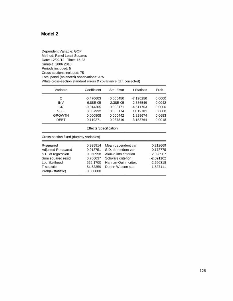
126

Model 2

Dependent Variable: GOP

Method: Panel Least Squares

Date: 12/02/12 Time: 15:23

Sample: 2006 2010

Periods included: 5

Cross-sections included: 75

Total panel (balanced) observations: 375

White cross-section standard errors & covariance (d.f. corrected) Variable Coefficient Std. Error t-Statistic Prob. C -0.470603 0.065450 -7.190250 0.0000

INV 6.88E-05 2.38E-05 2.886549 0.0042

CR -0.014305 0.003171 -4.511763 0.0000

SIZE 0.057932 0.005174 11.19781 0.0000

GROWTH 0.000808 0.000442 1.829674 0.0683

DEBT -0.119271 0.037819 -3.153764 0.0018 Effects Specification Cross-section fixed (dummy variables) R-squared 0.935914 Mean dependent var 0.212669

Adjusted R-squared 0.918751 S.D. dependent var 0.178775

S.E. of regression 0.050958 Akaike info criterion -2.928907

Sum squared resid 0.766037 Schwarz criterion -2.091162

Log likelihood 629.1700 Hannan-Quinn criter. -2.596318

F-statistic 54.53359 Durbin-Watson stat 1.637111

Prob(F-statistic) 0.000000

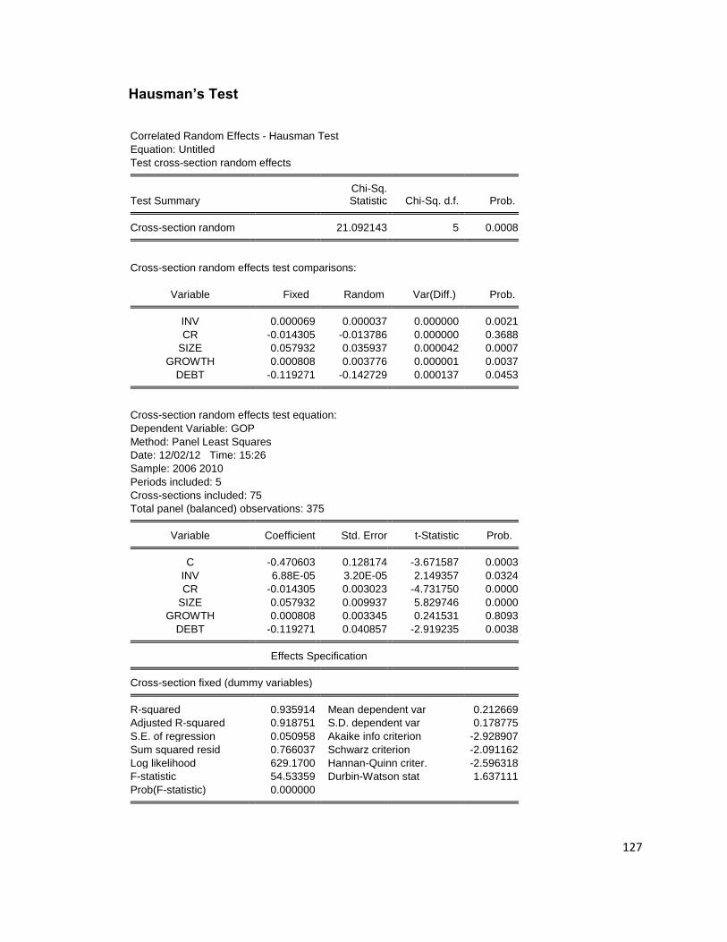
127

Hausman’s Test

Correlated Random Effects - Hausman Test

Equation: Untitled

Test cross-section random effects

Test Summary Chi-Sq. Statistic Chi-Sq. d.f. Prob.

Cross-section random 21.092143 5 0.0008

Cross-section random effects test comparisons:

Variable Fixed Random Var(Diff.) Prob. INV 0.000069 0.000037 0.000000 0.0021

CR -0.014305 -0.013786 0.000000 0.3688

SIZE 0.057932 0.035937 0.000042 0.0007

GROWTH 0.000808 0.003776 0.000001 0.0037

DEBT -0.119271 -0.142729 0.000137 0.0453

Cross-section random effects test equation:

Dependent Variable: GOP

Method: Panel Least Squares

Date: 12/02/12 Time: 15:26

Sample: 2006 2010

Periods included: 5

Cross-sections included: 75

Total panel (balanced) observations: 375 Variable Coefficient Std. Error t-Statistic Prob. C -0.470603 0.128174 -3.671587 0.0003

INV 6.88E-05 3.20E-05 2.149357 0.0324

CR -0.014305 0.003023 -4.731750 0.0000

SIZE 0.057932 0.009937 5.829746 0.0000

GROWTH 0.000808 0.003345 0.241531 0.8093

DEBT -0.119271 0.040857 -2.919235 0.0038 Effects Specification Cross-section fixed (dummy variables) R-squared 0.935914 Mean dependent var 0.212669

Adjusted R-squared 0.918751 S.D. dependent var 0.178775

S.E. of regression 0.050958 Akaike info criterion -2.928907

Sum squared resid 0.766037 Schwarz criterion -2.091162

Log likelihood 629.1700 Hannan-Quinn criter. -2.596318

F-statistic 54.53359 Durbin-Watson stat 1.637111

Prob(F-statistic) 0.000000

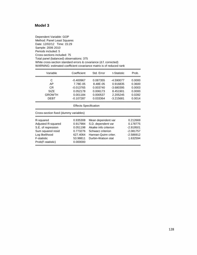
128

Model 3

Dependent Variable: GOP

Method: Panel Least Squares

Date: 12/02/12 Time: 15:29

Sample: 2006 2010

Periods included: 5

Cross-sections included: 75

Total panel (balanced) observations: 375

White cross-section standard errors & covariance (d.f. corrected)

WARNING: estimated coefficient covariance matrix is of reduced rank Variable Coefficient Std. Error t-Statistic Prob. C -0.400967 0.087355 -4.590077 0.0000

AP 7.78E-05 8.48E-05 0.916835 0.3600

CR -0.013765 0.003740 -3.680395 0.0003

SIZE 0.052178 0.006173 8.451901 0.0000

GROWTH 0.001184 0.000537 2.205245 0.0282

DEBT -0.107287 0.033364 -3.215681 0.0014 Effects Specification Cross-section fixed (dummy variables) R-squared 0.935308 Mean dependent var 0.212669

Adjusted R-squared 0.917984 S.D. dependent var 0.178775

S.E. of regression 0.051198 Akaike info criterion -2.919501

Sum squared resid 0.773276 Schwarz criterion -2.081757

Log likelihood 627.4064 Hannan-Quinn criter. -2.586912

F-statistic 53.98811 Durbin-Watson stat 1.632594

Prob(F-statistic) 0.000000

129

Hausman’s Test

Correlated Random Effects - Hausman Test

Equation: Untitled

Test cross-section random effects

Test Summary Chi-Sq. Statistic Chi-Sq. d.f. Prob.

Cross-section random 20.225446 5 0.0011

Cross-section random effects test comparisons:

Variable Fixed Random Var(Diff.) Prob. AP 0.000078 0.000040 0.000000 0.0039

CR -0.013765 -0.013462 0.000000 0.6062

SIZE 0.052178 0.033644 0.000035 0.0018

GROWTH 0.001184 0.003830 0.000001 0.0086

DEBT -0.107287 -0.136920 0.000136 0.0110

Cross-section random effects test equation:

Dependent Variable: GOP

Method: Panel Least Squares

Date: 12/02/12 Time: 15:32

Sample: 2006 2010

Periods included: 5

Cross-sections included: 75

Total panel (balanced) observations: 375 Variable Coefficient Std. Error t-Statistic Prob. C -0.400967 0.121774 -3.292722 0.0011

AP 7.78E-05 5.77E-05 1.347152 0.1790

CR -0.013765 0.003089 -4.456875 0.0000

SIZE 0.052178 0.009372 5.567336 0.0000

GROWTH 0.001184 0.003354 0.353069 0.7243

DEBT -0.107287 0.040550 -2.645795 0.0086 Effects Specification Cross-section fixed (dummy variables) R-squared 0.935308 Mean dependent var 0.212669

Adjusted R-squared 0.917984 S.D. dependent var 0.178775

S.E. of regression 0.051198 Akaike info criterion -2.919501

Sum squared resid 0.773276 Schwarz criterion -2.081757

Log likelihood 627.4064 Hannan-Quinn criter. -2.586912

F-statistic 53.98811 Durbin-Watson stat 1.632594

Prob(F-statistic) 0.000000

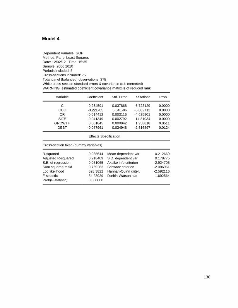
130

Model 4

Dependent Variable: GOP

Method: Panel Least Squares

Date: 12/02/12 Time: 15:35

Sample: 2006 2010

Periods included: 5

Cross-sections included: 75

Total panel (balanced) observations: 375

White cross-section standard errors & covariance (d.f. corrected)

WARNING: estimated coefficient covariance matrix is of reduced rank Variable Coefficient Std. Error t-Statistic Prob. C -0.254591 0.037868 -6.723129 0.0000

CCC -3.22E-05 6.34E-06 -5.082712 0.0000

CR -0.014412 0.003116 -4.625901 0.0000

SIZE 0.041349 0.002792 14.81034 0.0000

GROWTH 0.001845 0.000942 1.958818 0.0511

DEBT -0.087961 0.034948 -2.516897 0.0124 Effects Specification Cross-section fixed (dummy variables) R-squared 0.935644 Mean dependent var 0.212669

Adjusted R-squared 0.918409 S.D. dependent var 0.178775

S.E. of regression 0.051065 Akaike info criterion -2.924705

Sum squared resid 0.769263 Schwarz criterion -2.086961

Log likelihood 628.3822 Hannan-Quinn criter. -2.592116

F-statistic 54.28929 Durbin-Watson stat 1.692564

Prob(F-statistic) 0.000000

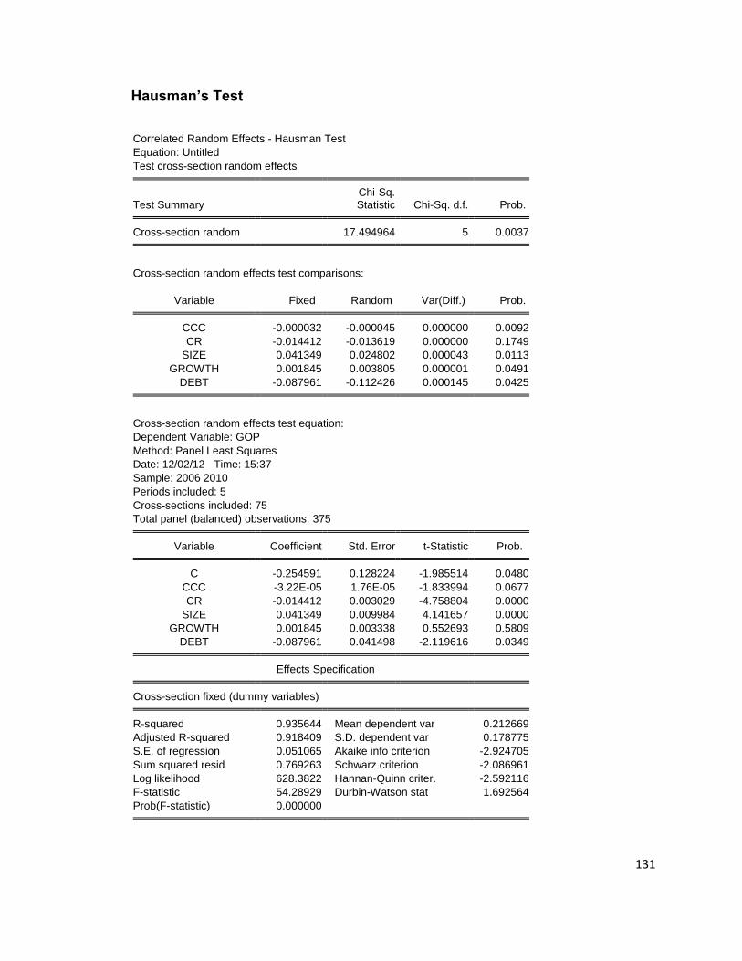
131

Hausman’s Test

Correlated Random Effects - Hausman Test

Equation: Untitled

Test cross-section random effects

Test Summary Chi-Sq. Statistic Chi-Sq. d.f. Prob.

Cross-section random 17.494964 5 0.0037

Cross-section random effects test comparisons:

Variable Fixed Random Var(Diff.) Prob. CCC -0.000032 -0.000045 0.000000 0.0092

CR -0.014412 -0.013619 0.000000 0.1749

SIZE 0.041349 0.024802 0.000043 0.0113

GROWTH 0.001845 0.003805 0.000001 0.0491

DEBT -0.087961 -0.112426 0.000145 0.0425

Cross-section random effects test equation:

Dependent Variable: GOP

Method: Panel Least Squares

Date: 12/02/12 Time: 15:37

Sample: 2006 2010

Periods included: 5

Cross-sections included: 75

Total panel (balanced) observations: 375 Variable Coefficient Std. Error t-Statistic Prob. C -0.254591 0.128224 -1.985514 0.0480

CCC -3.22E-05 1.76E-05 -1.833994 0.0677

CR -0.014412 0.003029 -4.758804 0.0000

SIZE 0.041349 0.009984 4.141657 0.0000

GROWTH 0.001845 0.003338 0.552693 0.5809

DEBT -0.087961 0.041498 -2.119616 0.0349 Effects Specification Cross-section fixed (dummy variables) R-squared 0.935644 Mean dependent var 0.212669

Adjusted R-squared 0.918409 S.D. dependent var 0.178775

S.E. of regression 0.051065 Akaike info criterion -2.924705

Sum squared resid 0.769263 Schwarz criterion -2.086961

Log likelihood 628.3822 Hannan-Quinn criter. -2.592116

F-statistic 54.28929 Durbin-Watson stat 1.692564

Prob(F-statistic) 0.000000

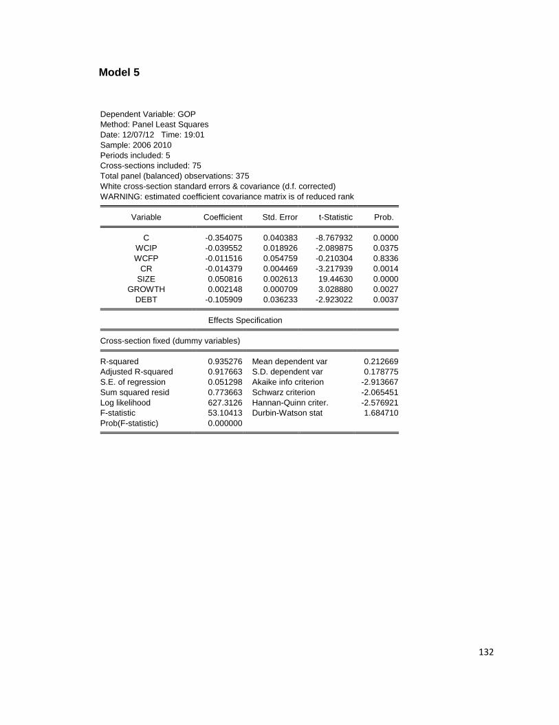
132

Model 5

Dependent Variable: GOP

Method: Panel Least Squares

Date: 12/07/12 Time: 19:01

Sample: 2006 2010

Periods included: 5

Cross-sections included: 75

Total panel (balanced) observations: 375

White cross-section standard errors & covariance (d.f. corrected)

WARNING: estimated coefficient covariance matrix is of reduced rank Variable Coefficient Std. Error t-Statistic Prob. C -0.354075 0.040383 -8.767932 0.0000

WCIP -0.039552 0.018926 -2.089875 0.0375

WCFP -0.011516 0.054759 -0.210304 0.8336

CR -0.014379 0.004469 -3.217939 0.0014

SIZE 0.050816 0.002613 19.44630 0.0000

GROWTH 0.002148 0.000709 3.028880 0.0027

DEBT -0.105909 0.036233 -2.923022 0.0037 Effects Specification Cross-section fixed (dummy variables) R-squared 0.935276 Mean dependent var 0.212669

Adjusted R-squared 0.917663 S.D. dependent var 0.178775

S.E. of regression 0.051298 Akaike info criterion -2.913667

Sum squared resid 0.773663 Schwarz criterion -2.065451

Log likelihood 627.3126 Hannan-Quinn criter. -2.576921

F-statistic 53.10413 Durbin-Watson stat 1.684710

Prob(F-statistic) 0.000000

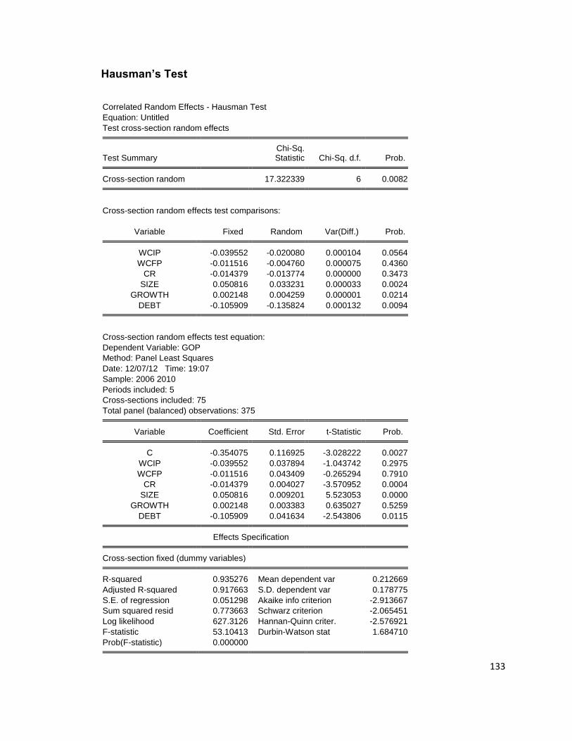
133

Hausman’s Test

Correlated Random Effects - Hausman Test

Equation: Untitled

Test cross-section random effects

Test Summary Chi-Sq. Statistic Chi-Sq. d.f. Prob.

Cross-section random 17.322339 6 0.0082

Cross-section random effects test comparisons:

Variable Fixed Random Var(Diff.) Prob. WCIP -0.039552 -0.020080 0.000104 0.0564

WCFP -0.011516 -0.004760 0.000075 0.4360

CR -0.014379 -0.013774 0.000000 0.3473

SIZE 0.050816 0.033231 0.000033 0.0024

GROWTH 0.002148 0.004259 0.000001 0.0214

DEBT -0.105909 -0.135824 0.000132 0.0094

Cross-section random effects test equation:

Dependent Variable: GOP

Method: Panel Least Squares

Date: 12/07/12 Time: 19:07

Sample: 2006 2010

Periods included: 5

Cross-sections included: 75

Total panel (balanced) observations: 375 Variable Coefficient Std. Error t-Statistic Prob. C -0.354075 0.116925 -3.028222 0.0027

WCIP -0.039552 0.037894 -1.043742 0.2975

WCFP -0.011516 0.043409 -0.265294 0.7910

CR -0.014379 0.004027 -3.570952 0.0004

SIZE 0.050816 0.009201 5.523053 0.0000

GROWTH 0.002148 0.003383 0.635027 0.5259

DEBT -0.105909 0.041634 -2.543806 0.0115 Effects Specification Cross-section fixed (dummy variables) R-squared 0.935276 Mean dependent var 0.212669

Adjusted R-squared 0.917663 S.D. dependent var 0.178775

S.E. of regression 0.051298 Akaike info criterion -2.913667

Sum squared resid 0.773663 Schwarz criterion -2.065451

Log likelihood 627.3126 Hannan-Quinn criter. -2.576921

F-statistic 53.10413 Durbin-Watson stat 1.684710

Prob(F-statistic) 0.000000

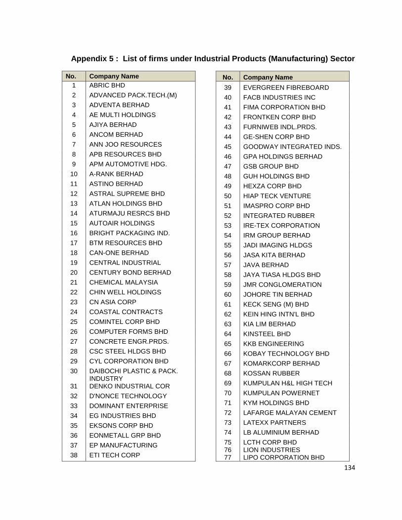
134

Appendix 5 : List of firms under Industrial Products (Manufacturing) Sector

No. Company Name

1 ABRIC BHD

2 ADVANCED PACK.TECH.(M)

3 ADVENTA BERHAD

4 AE MULTI HOLDINGS

5 AJIYA BERHAD

6 ANCOM BERHAD

7 ANN JOO RESOURCES

8 APB RESOURCES BHD

9 APM AUTOMOTIVE HDG.

10 A-RANK BERHAD

11 ASTINO BERHAD

12 ASTRAL SUPREME BHD

13 ATLAN HOLDINGS BHD

14 ATURMAJU RESRCS BHD

15 AUTOAIR HOLDINGS

16 BRIGHT PACKAGING IND.

17 BTM RESOURCES BHD

18 CAN-ONE BERHAD

19 CENTRAL INDUSTRIAL

20 CENTURY BOND BERHAD

21 CHEMICAL MALAYSIA

22 CHIN WELL HOLDINGS

23 CN ASIA CORP

24 COASTAL CONTRACTS

25 COMINTEL CORP BHD

26 COMPUTER FORMS BHD

27 CONCRETE ENGR.PRDS.

28 CSC STEEL HLDGS BHD

29 CYL CORPORATION BHD

30 DAIBOCHI PLASTIC & PACK. INDUSTRY

31 DENKO INDUSTRIAL COR

32 D'NONCE TECHNOLOGY

33 DOMINANT ENTERPRISE

34 EG INDUSTRIES BHD

35 EKSONS CORP BHD

36 EONMETALL GRP BHD

37 EP MANUFACTURING

38 ETI TECH CORP

No. Company Name

39 EVERGREEN FIBREBOARD

40 FACB INDUSTRIES INC

41 FIMA CORPORATION BHD

42 FRONTKEN CORP BHD

43 FURNIWEB INDL.PRDS.

44 GE-SHEN CORP BHD

45 GOODWAY INTEGRATED INDS.

46 GPA HOLDINGS BERHAD

47 GSB GROUP BHD

48 GUH HOLDINGS BHD

49 HEXZA CORP BHD

50 HIAP TECK VENTURE

51 IMASPRO CORP BHD

52 INTEGRATED RUBBER

53 IRE-TEX CORPORATION

54 IRM GROUP BERHAD

55 JADI IMAGING HLDGS

56 JASA KITA BERHAD

57 JAVA BERHAD

58 JAYA TIASA HLDGS BHD

59 JMR CONGLOMERATION

60 JOHORE TIN BERHAD

61 KECK SENG (M) BHD

62 KEIN HING INTN'L BHD

63 KIA LIM BERHAD

64 KINSTEEL BHD

65 KKB ENGINEERING

66 KOBAY TECHNOLOGY BHD

67 KOMARKCORP BERHAD

68 KOSSAN RUBBER

69 KUMPULAN H&L HIGH TECH

70 KUMPULAN POWERNET

71 KYM HOLDINGS BHD

72 LAFARGE MALAYAN CEMENT

73 LATEXX PARTNERS

74 LB ALUMINIUM BERHAD

75 LCTH CORP BHD 76 77

LION INDUSTRIES LIPO CORPORATION BHD

135

No. Company Name

78 MAJOR TEAM HOLDINGS

79 MALAYSIA AICA BERHAD

80 MALAYSIA PACKAGING IND.

81 MALAYSIA SMELTING

82 MALAYSIAN AE MODELS HDG.

83 MAXTRAL INDUSTRY BHD

84 MERCURY INDUSTRIES

85 METAL RECLAMATION

86 METROD HOLDINGS

87 MIECO CHIPBOARD

88 MUDA HOLDINGS BERHAD

89 MULTICODE ELTN.INDS.

90 NWP HOLDINGS BERHAD

91 NYLEX (MALAYSIA) BHD

92 OKA CORPORATION BHD

93 P.I.E. INDUSTRIAL

94 PELANGI PUBLISHING GP.

95 PENSONIC HOLDINGS

96 PERMAJU INDUSTRIES

97 PERSTIMA.MAL.(PERSTIMA)

98 PETRON MAL.REFN.& MKTG.

99 PNE PCB BERHAD

100 POLY GLASS FIBRE (M)

101 PREMIUM NALFIN

102 PRESS METAL BERHAD

103 PRICEWORTH INTERNATIONAL

104 QUALITY CONCRETE HDG.

105 SAPURA INDUSTRIAL

106 SARAWAK CONS.INDS.

107 SCIENTEX BERHAD

108 SEACERA GROUP

109 SIG GASES BERHAD

110 SKB SHUTTERS CORP

111 SKP RESOURCES BERHAD

112 SMIS CORPORATION BHD

No. Company Name

113 STONE MASTER CORPOR

114 SUBUR TIASA HOLDINGS

115 SUPER ENTERPRISE HDG.

116 SUPERMAX CORP BHD

117 TA WIN HOLDINGS

118 TASEK CORPORATION

119 TECK GUAN PERDANA

120 TECNIC GROUP BERHAD

121 TEKALA CORP BHD

122 TIEN WAH PRESS HOLDINGS

123 TIGER SYNERGY BERHAD

124 TIMBERWELL BERHAD

125 TOYO INK GROUP BHD

126 UAC BERHAD

127 UCHI TECHNOLOGIES

128 UMS-NEIKEN GROUP

129 UNITED BINTANG BHD

130 UNITED U-LI CORPOR

131 V.S. INDUSTRY BERHAD

132 VERSATILE CREATIVE

133 WAH SEONG CORP

134 WATTA HOLDINGS

135 WAWASAN TKH HOLDINGS

136 WEIDA (M) BERHAD

137 WONG ENGINEERING

138 WTK HOLDINGS BHD

139 YA HORNG ELECTRONIC (M)

140 YI-LAI BHD

141 YLI HOLDINGS BHD

142 YOKOHAMA INDUSTRIES

143 YUNG KONG GALVANISING INDS.

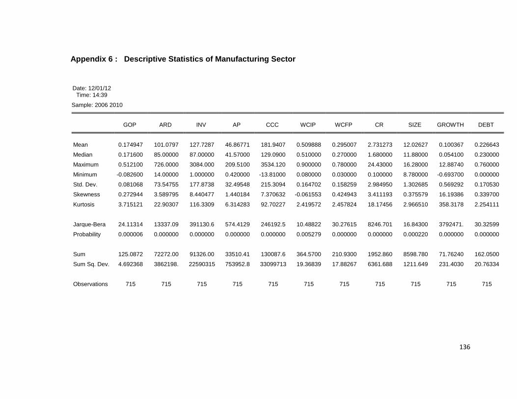
136

Appendix 6 : Descriptive Statistics of Manufacturing Sector

Date: 12/01/12

Time: 14:39

Sample: 2006 2010 GOP ARD INV AP CCC WCIP WCFP CR SIZE GROWTH DEBT

Mean 0.174947 101.0797 127.7287 46.86771 181.9407 0.509888 0.295007 2.731273 12.02627 0.100367 0.226643

Median 0.171600 85.00000 87.00000 41.57000 129.0900 0.510000 0.270000 1.680000 11.88000 0.054100 0.230000

Maximum 0.512100 726.0000 3084.000 209.5100 3534.120 0.900000 0.780000 24.43000 16.28000 12.88740 0.760000

Minimum -0.082600 14.00000 1.000000 0.420000 -13.81000 0.080000 0.030000 0.100000 8.780000 -0.693700 0.000000

Std. Dev. 0.081068 73.54755 177.8738 32.49548 215.3094 0.164702 0.158259 2.984950 1.302685 0.569292 0.170530

Skewness 0.272944 3.589795 8.440477 1.440184 7.370632 -0.061553 0.424943 3.411193 0.375579 16.19386 0.339700

Kurtosis 3.715121 22.90307 116.3309 6.314283 92.70227 2.419572 2.457824 18.17456 2.966510 358.3178 2.254111

Jarque-Bera 24.11314 13337.09 391130.6 574.4129 246192.5 10.48822 30.27615 8246.701 16.84300 3792471. 30.32599

Probability 0.000006 0.000000 0.000000 0.000000 0.000000 0.005279 0.000000 0.000000 0.000220 0.000000 0.000000

Sum 125.0872 72272.00 91326.00 33510.41 130087.6 364.5700 210.9300 1952.860 8598.780 71.76240 162.0500

Sum Sq. Dev. 4.692368 3862198. 22590315 753952.8 33099713 19.36839 17.88267 6361.688 1211.649 231.4030 20.76334

Observations 715 715 715 715 715 715 715 715 715 715 715

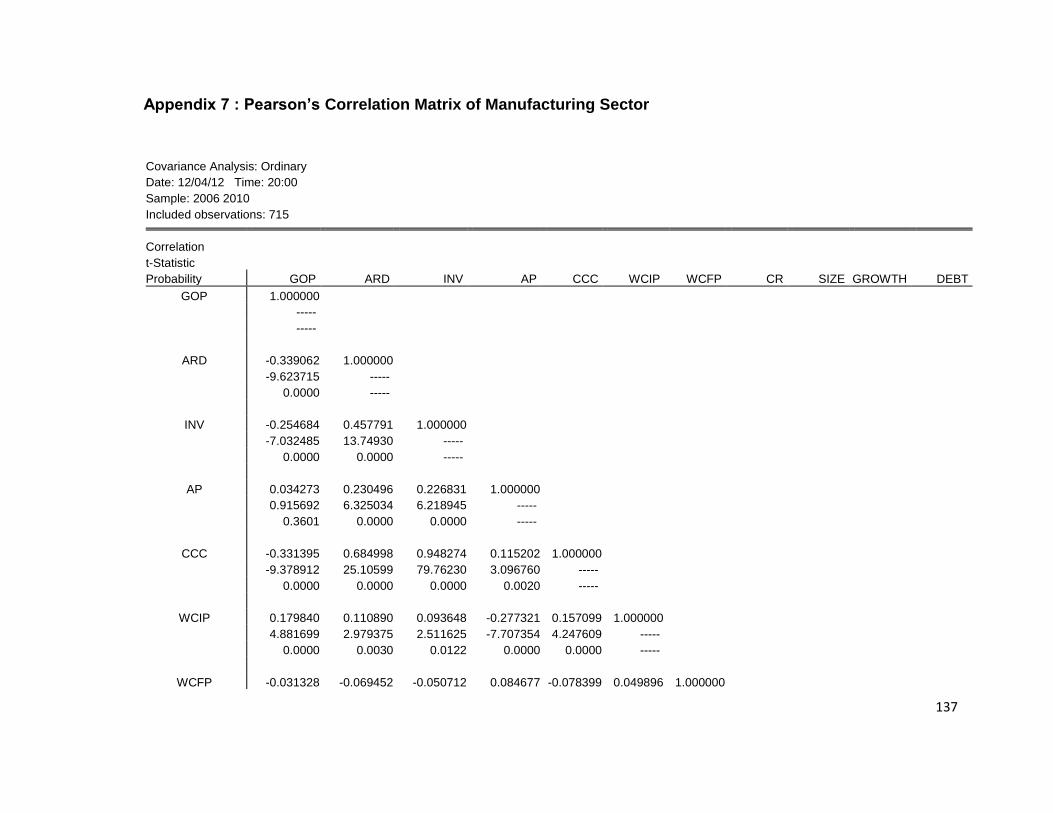
137

Appendix 7 : Pearson’s Correlation Matrix of Manufacturing Sector

Covariance Analysis: Ordinary

Date: 12/04/12 Time: 20:00

Sample: 2006 2010

Included observations: 715 Correlation

t-Statistic

Probability GOP ARD INV AP CCC WCIP WCFP CR SIZE GROWTH DEBT

GOP 1.000000

-----

-----

ARD -0.339062 1.000000

-9.623715 -----

0.0000 -----

INV -0.254684 0.457791 1.000000

-7.032485 13.74930 -----

0.0000 0.0000 -----

AP 0.034273 0.230496 0.226831 1.000000

0.915692 6.325034 6.218945 -----

0.3601 0.0000 0.0000 -----

CCC -0.331395 0.684998 0.948274 0.115202 1.000000

-9.378912 25.10599 79.76230 3.096760 -----

0.0000 0.0000 0.0000 0.0020 -----

WCIP 0.179840 0.110890 0.093648 -0.277321 0.157099 1.000000

4.881699 2.979375 2.511625 -7.707354 4.247609 -----

0.0000 0.0030 0.0122 0.0000 0.0000 -----

WCFP -0.031328 -0.069452 -0.050712 0.084677 -0.078399 0.049896 1.000000

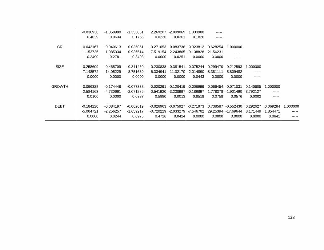
138

-0.836936 -1.858988 -1.355861 2.269207 -2.099869 1.333988 -----

0.4029 0.0634 0.1756 0.0236 0.0361 0.1826 -----

CR -0.043167 0.040613 0.035051 -0.271053 0.083738 0.323812 -0.628254 1.000000

-1.153726 1.085334 0.936514 -7.519154 2.243865 9.138828 -21.56231 -----

0.2490 0.2781 0.3493 0.0000 0.0251 0.0000 0.0000 -----

SIZE 0.258609 -0.465709 -0.311450 -0.230838 -0.381541 0.075244 0.299470 -0.212593 1.000000

7.148572 -14.05229 -8.751639 -6.334941 -11.02170 2.014890 8.381111 -5.809482 -----

0.0000 0.0000 0.0000 0.0000 0.0000 0.0443 0.0000 0.0000 -----

GROWTH 0.096328 -0.174448 -0.077338 -0.020291 -0.120419 -0.006999 0.066454 -0.071031 0.140605 1.000000

2.584163 -4.730661 -2.071289 -0.541920 -3.238997 -0.186897 1.778378 -1.901490 3.792127 -----

0.0100 0.0000 0.0387 0.5880 0.0013 0.8518 0.0758 0.0576 0.0002 -----

DEBT -0.184220 -0.084197 -0.062019 -0.026963 -0.075927 -0.271973 0.738587 -0.552430 0.292627 0.069284 1.000000

-5.004721 -2.256257 -1.659217 -0.720229 -2.033279 -7.546702 29.25394 -17.69644 8.171449 1.854471 -----

0.0000 0.0244 0.0975 0.4716 0.0424 0.0000 0.0000 0.0000 0.0000 0.0641 -----

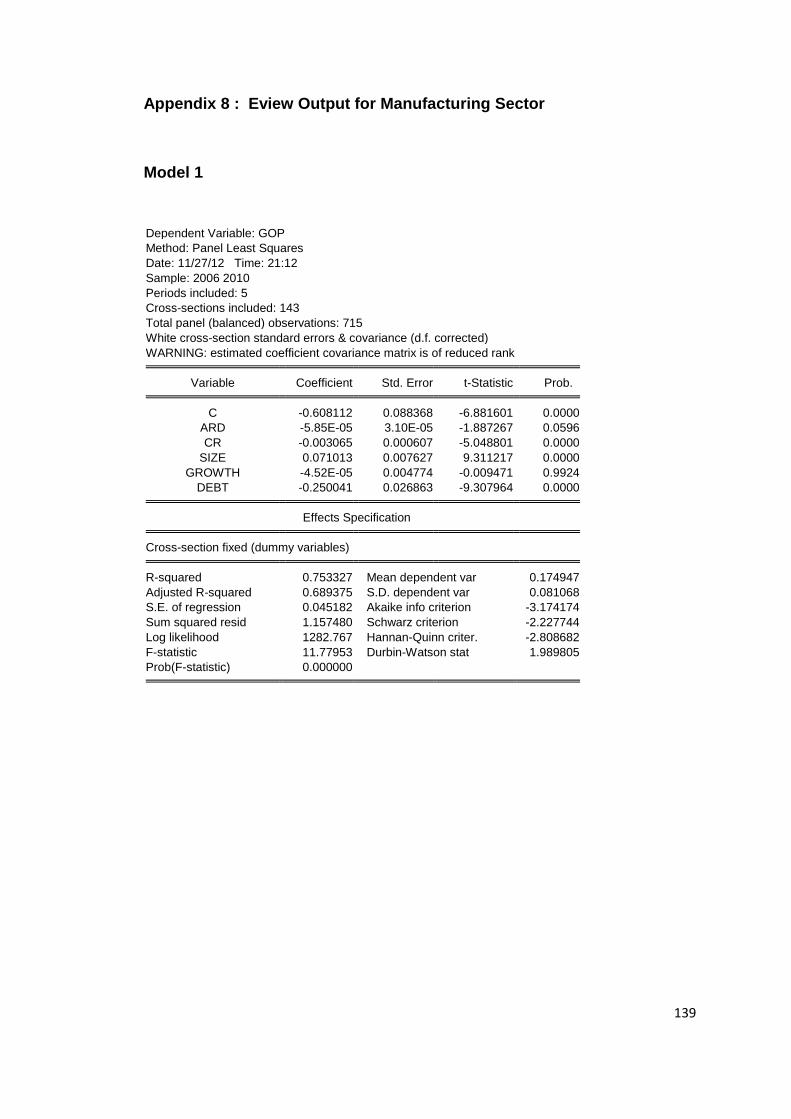
139

Appendix 8 : Eview Output for Manufacturing Sector

Model 1

Dependent Variable: GOP

Method: Panel Least Squares

Date: 11/27/12 Time: 21:12

Sample: 2006 2010

Periods included: 5

Cross-sections included: 143

Total panel (balanced) observations: 715

White cross-section standard errors & covariance (d.f. corrected)

WARNING: estimated coefficient covariance matrix is of reduced rank Variable Coefficient Std. Error t-Statistic Prob. C -0.608112 0.088368 -6.881601 0.0000

ARD -5.85E-05 3.10E-05 -1.887267 0.0596

CR -0.003065 0.000607 -5.048801 0.0000

SIZE 0.071013 0.007627 9.311217 0.0000

GROWTH -4.52E-05 0.004774 -0.009471 0.9924

DEBT -0.250041 0.026863 -9.307964 0.0000 Effects Specification Cross-section fixed (dummy variables) R-squared 0.753327 Mean dependent var 0.174947

Adjusted R-squared 0.689375 S.D. dependent var 0.081068

S.E. of regression 0.045182 Akaike info criterion -3.174174

Sum squared resid 1.157480 Schwarz criterion -2.227744

Log likelihood 1282.767 Hannan-Quinn criter. -2.808682

F-statistic 11.77953 Durbin-Watson stat 1.989805

Prob(F-statistic) 0.000000

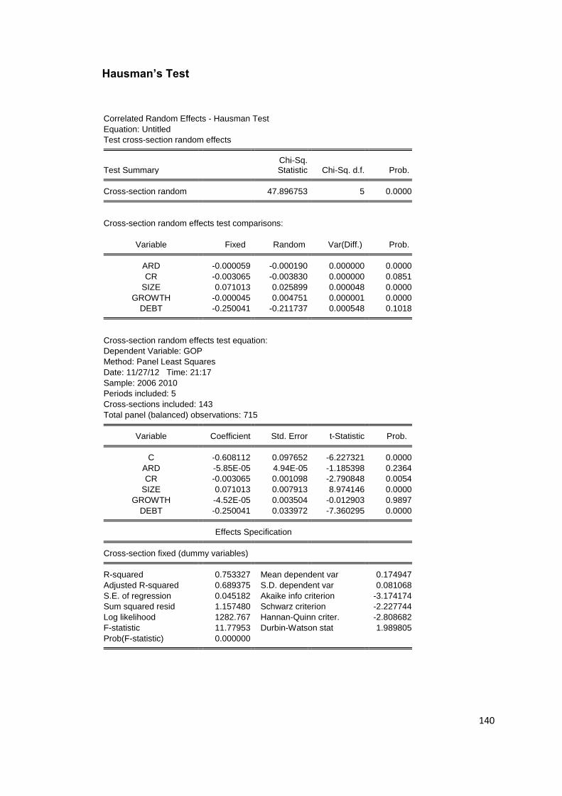
140

Hausman’s Test

Correlated Random Effects - Hausman Test

Equation: Untitled

Test cross-section random effects

Test Summary Chi-Sq. Statistic Chi-Sq. d.f. Prob.

Cross-section random 47.896753 5 0.0000

Cross-section random effects test comparisons:

Variable Fixed Random Var(Diff.) Prob. ARD -0.000059 -0.000190 0.000000 0.0000

CR -0.003065 -0.003830 0.000000 0.0851

SIZE 0.071013 0.025899 0.000048 0.0000

GROWTH -0.000045 0.004751 0.000001 0.0000

DEBT -0.250041 -0.211737 0.000548 0.1018

Cross-section random effects test equation:

Dependent Variable: GOP

Method: Panel Least Squares

Date: 11/27/12 Time: 21:17

Sample: 2006 2010

Periods included: 5

Cross-sections included: 143

Total panel (balanced) observations: 715 Variable Coefficient Std. Error t-Statistic Prob. C -0.608112 0.097652 -6.227321 0.0000

ARD -5.85E-05 4.94E-05 -1.185398 0.2364

CR -0.003065 0.001098 -2.790848 0.0054

SIZE 0.071013 0.007913 8.974146 0.0000

GROWTH -4.52E-05 0.003504 -0.012903 0.9897

DEBT -0.250041 0.033972 -7.360295 0.0000 Effects Specification Cross-section fixed (dummy variables) R-squared 0.753327 Mean dependent var 0.174947

Adjusted R-squared 0.689375 S.D. dependent var 0.081068

S.E. of regression 0.045182 Akaike info criterion -3.174174

Sum squared resid 1.157480 Schwarz criterion -2.227744

Log likelihood 1282.767 Hannan-Quinn criter. -2.808682

F-statistic 11.77953 Durbin-Watson stat 1.989805

Prob(F-statistic) 0.000000

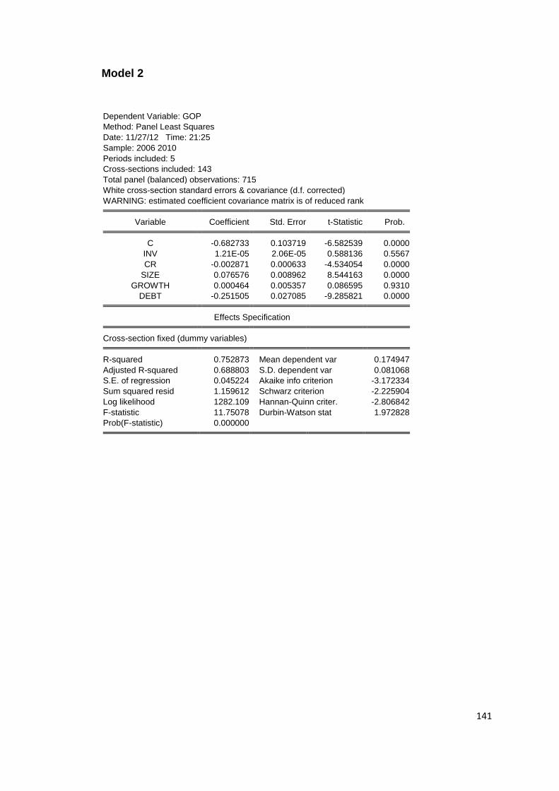
141

Model 2

Dependent Variable: GOP

Method: Panel Least Squares

Date: 11/27/12 Time: 21:25

Sample: 2006 2010

Periods included: 5

Cross-sections included: 143

Total panel (balanced) observations: 715

White cross-section standard errors & covariance (d.f. corrected)

WARNING: estimated coefficient covariance matrix is of reduced rank Variable Coefficient Std. Error t-Statistic Prob. C -0.682733 0.103719 -6.582539 0.0000

INV 1.21E-05 2.06E-05 0.588136 0.5567

CR -0.002871 0.000633 -4.534054 0.0000

SIZE 0.076576 0.008962 8.544163 0.0000

GROWTH 0.000464 0.005357 0.086595 0.9310

DEBT -0.251505 0.027085 -9.285821 0.0000 Effects Specification Cross-section fixed (dummy variables) R-squared 0.752873 Mean dependent var 0.174947

Adjusted R-squared 0.688803 S.D. dependent var 0.081068

S.E. of regression 0.045224 Akaike info criterion -3.172334

Sum squared resid 1.159612 Schwarz criterion -2.225904

Log likelihood 1282.109 Hannan-Quinn criter. -2.806842

F-statistic 11.75078 Durbin-Watson stat 1.972828

Prob(F-statistic) 0.000000

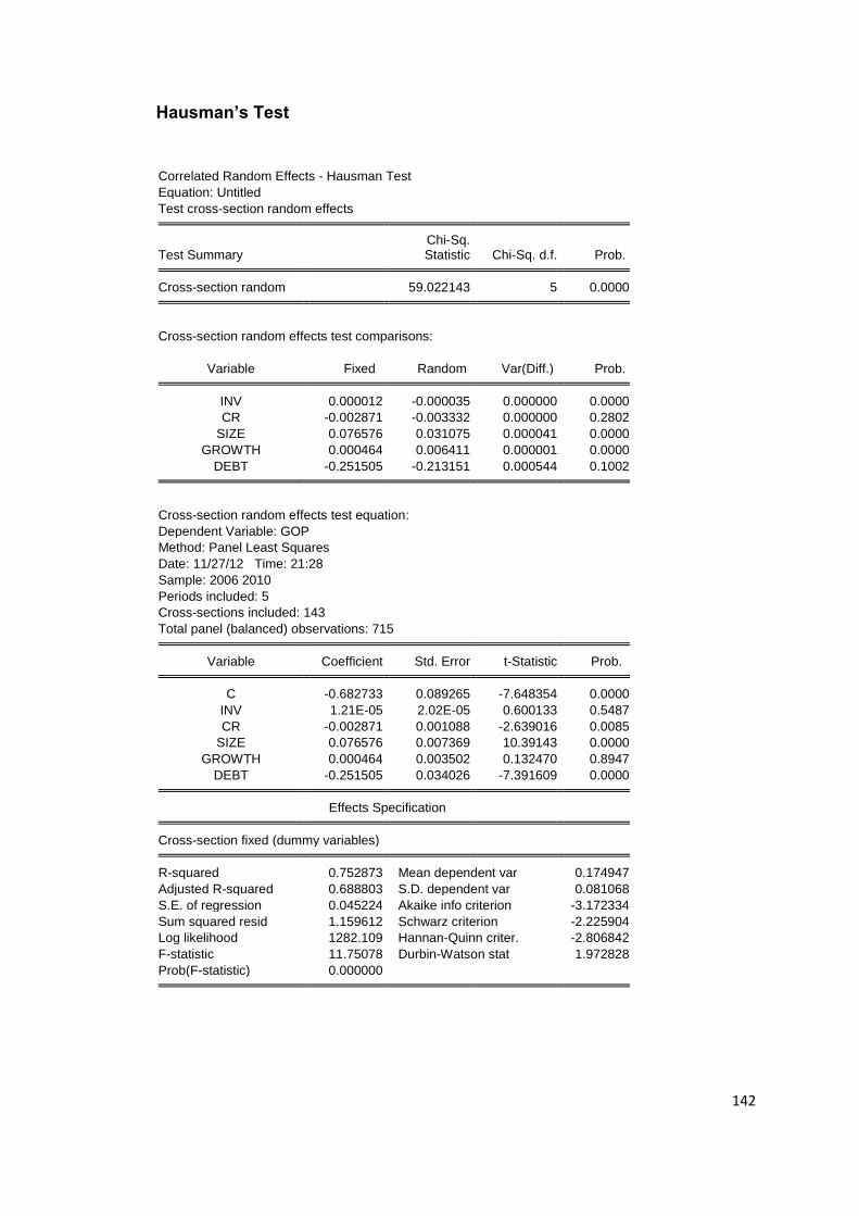
142

Hausman’s Test

Correlated Random Effects - Hausman Test

Equation: Untitled

Test cross-section random effects

Test Summary Chi-Sq. Statistic Chi-Sq. d.f. Prob.

Cross-section random 59.022143 5 0.0000

Cross-section random effects test comparisons:

Variable Fixed Random Var(Diff.) Prob. INV 0.000012 -0.000035 0.000000 0.0000

CR -0.002871 -0.003332 0.000000 0.2802

SIZE 0.076576 0.031075 0.000041 0.0000

GROWTH 0.000464 0.006411 0.000001 0.0000

DEBT -0.251505 -0.213151 0.000544 0.1002

Cross-section random effects test equation:

Dependent Variable: GOP

Method: Panel Least Squares

Date: 11/27/12 Time: 21:28

Sample: 2006 2010

Periods included: 5

Cross-sections included: 143

Total panel (balanced) observations: 715 Variable Coefficient Std. Error t-Statistic Prob. C -0.682733 0.089265 -7.648354 0.0000

INV 1.21E-05 2.02E-05 0.600133 0.5487

CR -0.002871 0.001088 -2.639016 0.0085

SIZE 0.076576 0.007369 10.39143 0.0000

GROWTH 0.000464 0.003502 0.132470 0.8947

DEBT -0.251505 0.034026 -7.391609 0.0000 Effects Specification Cross-section fixed (dummy variables) R-squared 0.752873 Mean dependent var 0.174947

Adjusted R-squared 0.688803 S.D. dependent var 0.081068

S.E. of regression 0.045224 Akaike info criterion -3.172334

Sum squared resid 1.159612 Schwarz criterion -2.225904

Log likelihood 1282.109 Hannan-Quinn criter. -2.806842

F-statistic 11.75078 Durbin-Watson stat 1.972828

Prob(F-statistic) 0.000000

143

Model 3

Dependent Variable: GOP

Method: Panel Least Squares

Date: 11/27/12 Time: 21:31

Sample: 2006 2010

Periods included: 5

Cross-sections included: 143

Total panel (balanced) observations: 715

White cross-section standard errors & covariance (d.f. corrected)

WARNING: estimated coefficient covariance matrix is of reduced rank Variable Coefficient Std. Error t-Statistic Prob. C -0.710946 0.117026 -6.075135 0.0000

AP 0.000190 0.000157 1.206945 0.2280

CR -0.002491 0.000522 -4.769546 0.0000

SIZE 0.078126 0.009377 8.331737 0.0000

GROWTH 0.000458 0.004899 0.093429 0.9256

DEBT -0.246248 0.024076 -10.22791 0.0000 Effects Specification Cross-section fixed (dummy variables) R-squared 0.754238 Mean dependent var 0.174947

Adjusted R-squared 0.690522 S.D. dependent var 0.081068

S.E. of regression 0.045098 Akaike info criterion -3.177875

Sum squared resid 1.153204 Schwarz criterion -2.231445

Log likelihood 1284.090 Hannan-Quinn criter. -2.812383

F-statistic 11.83750 Durbin-Watson stat 1.970876

Prob(F-statistic) 0.000000

144

Hausman’s Test

Correlated Random Effects - Hausman Test

Equation: Untitled

Test cross-section random effects

Test Summary Chi-Sq. Statistic Chi-Sq. d.f. Prob.

Cross-section random 53.464356 5 0.0000

Cross-section random effects test comparisons:

Variable Fixed Random Var(Diff.) Prob. AP 0.000190 0.000135 0.000000 0.2292

CR -0.002491 -0.002917 0.000000 0.2798

SIZE 0.078126 0.034990 0.000038 0.0000

GROWTH 0.000458 0.007155 0.000001 0.0000

DEBT -0.246248 -0.213945 0.000522 0.1574

Cross-section random effects test equation:

Dependent Variable: GOP

Method: Panel Least Squares

Date: 11/27/12 Time: 21:34

Sample: 2006 2010

Periods included: 5

Cross-sections included: 143

Total panel (balanced) observations: 715 Variable Coefficient Std. Error t-Statistic Prob. C -0.710946 0.087841 -8.093525 0.0000

AP 0.000190 0.000101 1.874189 0.0614

CR -0.002491 0.001104 -2.256040 0.0244

SIZE 0.078126 0.007191 10.86378 0.0000

GROWTH 0.000458 0.003485 0.131331 0.8956

DEBT -0.246248 0.033987 -7.245363 0.0000 Effects Specification Cross-section fixed (dummy variables) R-squared 0.754238 Mean dependent var 0.174947

Adjusted R-squared 0.690522 S.D. dependent var 0.081068

S.E. of regression 0.045098 Akaike info criterion -3.177875

Sum squared resid 1.153204 Schwarz criterion -2.231445

Log likelihood 1284.090 Hannan-Quinn criter. -2.812383

F-statistic 11.83750 Durbin-Watson stat 1.970876

Prob(F-statistic) 0.000000

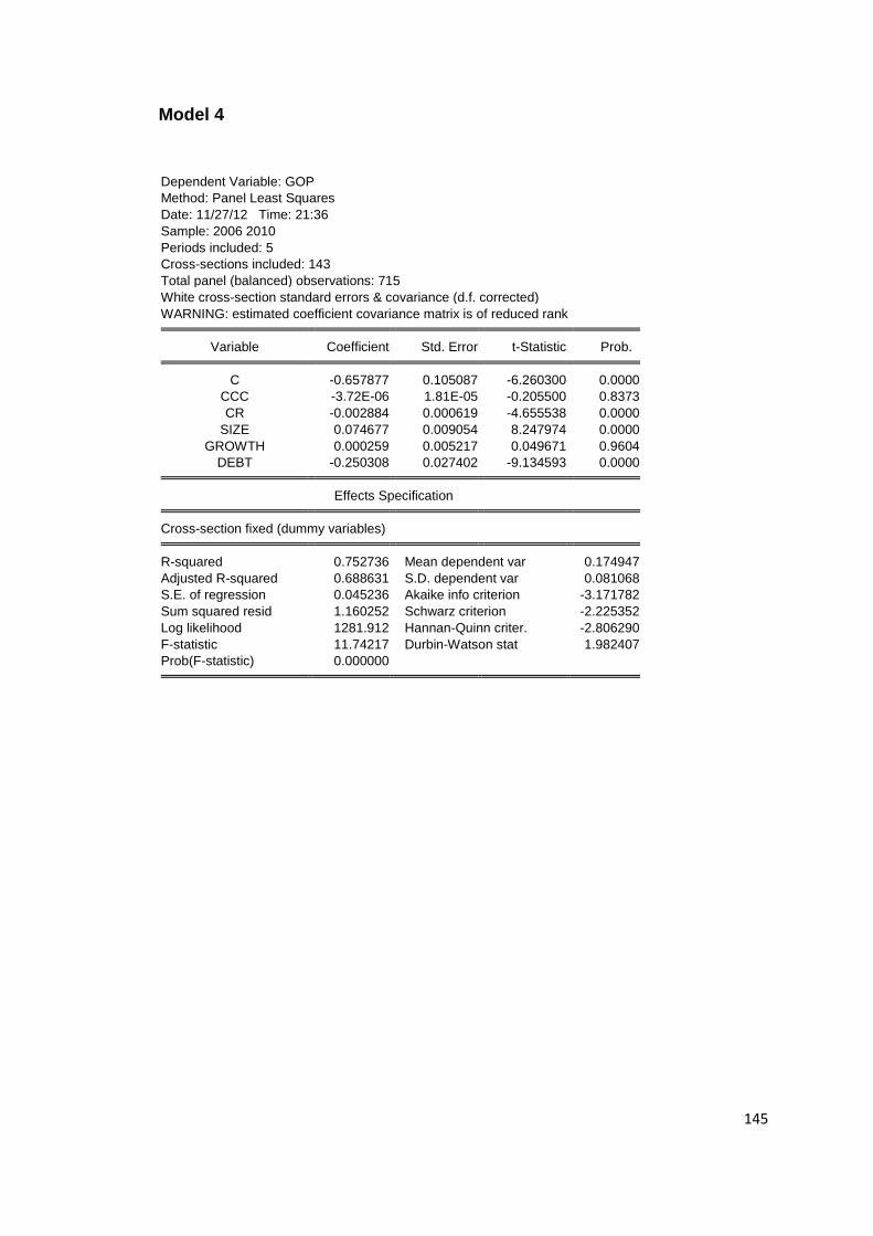
145

Model 4

Dependent Variable: GOP

Method: Panel Least Squares

Date: 11/27/12 Time: 21:36

Sample: 2006 2010

Periods included: 5

Cross-sections included: 143

Total panel (balanced) observations: 715

White cross-section standard errors & covariance (d.f. corrected)

WARNING: estimated coefficient covariance matrix is of reduced rank Variable Coefficient Std. Error t-Statistic Prob. C -0.657877 0.105087 -6.260300 0.0000

CCC -3.72E-06 1.81E-05 -0.205500 0.8373

CR -0.002884 0.000619 -4.655538 0.0000

SIZE 0.074677 0.009054 8.247974 0.0000

GROWTH 0.000259 0.005217 0.049671 0.9604

DEBT -0.250308 0.027402 -9.134593 0.0000 Effects Specification Cross-section fixed (dummy variables) R-squared 0.752736 Mean dependent var 0.174947

Adjusted R-squared 0.688631 S.D. dependent var 0.081068

S.E. of regression 0.045236 Akaike info criterion -3.171782

Sum squared resid 1.160252 Schwarz criterion -2.225352

Log likelihood 1281.912 Hannan-Quinn criter. -2.806290

F-statistic 11.74217 Durbin-Watson stat 1.982407

Prob(F-statistic) 0.000000

146

Hausman’s Test

Correlated Random Effects - Hausman Test

Equation: Untitled

Test cross-section random effects

Test Summary Chi-Sq. Statistic Chi-Sq. d.f. Prob.

Cross-section random 56.878507 5 0.0000

Cross-section random effects test comparisons:

Variable Fixed Random Var(Diff.) Prob. CCC -0.000004 -0.000052 0.000000 0.0000

CR -0.002884 -0.003363 0.000000 0.2709

SIZE 0.074677 0.028245 0.000044 0.0000

GROWTH 0.000259 0.005624 0.000001 0.0000

DEBT -0.250308 -0.209424 0.000556 0.0831

Cross-section random effects test equation:

Dependent Variable: GOP

Method: Panel Least Squares

Date: 11/27/12 Time: 21:39

Sample: 2006 2010

Periods included: 5

Cross-sections included: 143

Total panel (balanced) observations: 715 Variable Coefficient Std. Error t-Statistic Prob. C -0.657877 0.092354 -7.123418 0.0000

CCC -3.72E-06 1.71E-05 -0.217078 0.8282

CR -0.002884 0.001089 -2.649049 0.0083

SIZE 0.074677 0.007594 9.833775 0.0000

GROWTH 0.000259 0.003507 0.073889 0.9411

DEBT -0.250308 0.034053 -7.350594 0.0000 Effects Specification Cross-section fixed (dummy variables) R-squared 0.752736 Mean dependent var 0.174947

Adjusted R-squared 0.688631 S.D. dependent var 0.081068

S.E. of regression 0.045236 Akaike info criterion -3.171782

Sum squared resid 1.160252 Schwarz criterion -2.225352

Log likelihood 1281.912 Hannan-Quinn criter. -2.806290

F-statistic 11.74217 Durbin-Watson stat 1.982407

Prob(F-statistic) 0.000000

147

Model 5

Dependent Variable: GOP

Method: Panel Least Squares

Date: 12/07/12 Time: 17:48

Sample: 2006 2010

Periods included: 5

Cross-sections included: 143

Total panel (balanced) observations: 715

White cross-section standard errors & covariance (d.f. corrected)

WARNING: estimated coefficient covariance matrix is of reduced rank Variable Coefficient Std. Error t-Statistic Prob. C -0.709407 0.065907 -10.76378 0.0000

WCIP 0.177296 0.033028 5.367987 0.0000

WCFP -0.123432 0.033917 -3.639187 0.0003

CR -0.004897 0.001176 -4.165119 0.0000

SIZE 0.070162 0.004565 15.36978 0.0000

GROWTH -0.000457 0.006165 -0.074177 0.9409 Effects Specification Cross-section fixed (dummy variables) R-squared 0.742706 Mean dependent var 0.174947

Adjusted R-squared 0.676000 S.D. dependent var 0.081068

S.E. of regression 0.046144 Akaike info criterion -3.132016

Sum squared resid 1.207320 Schwarz criterion -2.185586

Log likelihood 1267.696 Hannan-Quinn criter. -2.766524

F-statistic 11.13402 Durbin-Watson stat 1.931575

Prob(F-statistic) 0.000000

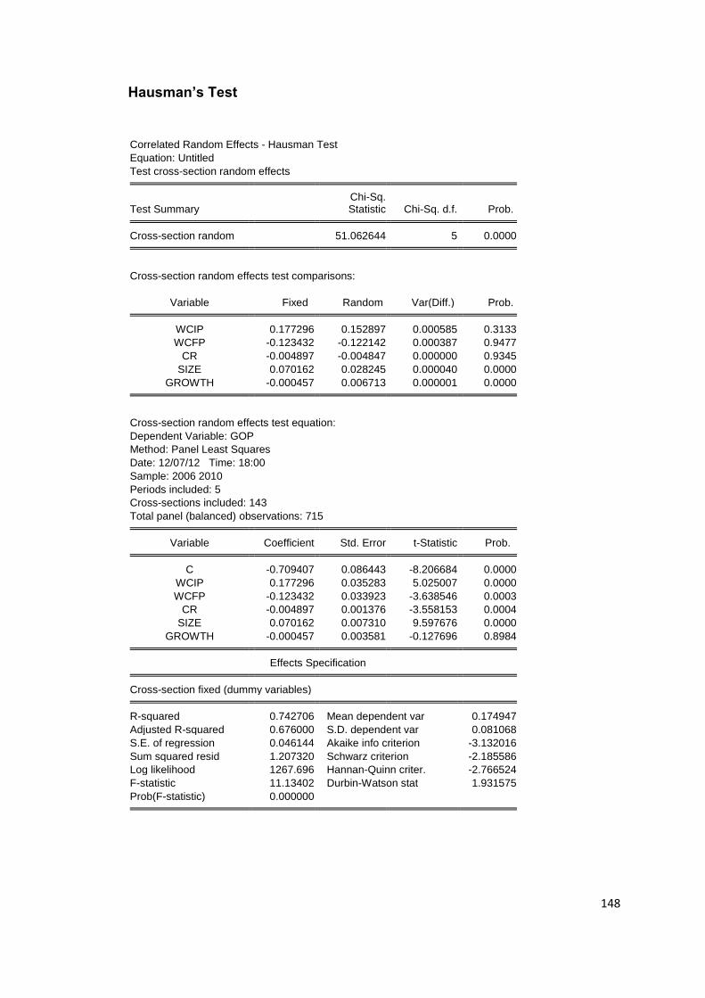
148

Hausman’s Test

Correlated Random Effects - Hausman Test

Equation: Untitled

Test cross-section random effects

Test Summary Chi-Sq. Statistic Chi-Sq. d.f. Prob.

Cross-section random 51.062644 5 0.0000

Cross-section random effects test comparisons:

Variable Fixed Random Var(Diff.) Prob. WCIP 0.177296 0.152897 0.000585 0.3133

WCFP -0.123432 -0.122142 0.000387 0.9477

CR -0.004897 -0.004847 0.000000 0.9345

SIZE 0.070162 0.028245 0.000040 0.0000

GROWTH -0.000457 0.006713 0.000001 0.0000

Cross-section random effects test equation:

Dependent Variable: GOP

Method: Panel Least Squares

Date: 12/07/12 Time: 18:00

Sample: 2006 2010

Periods included: 5

Cross-sections included: 143

Total panel (balanced) observations: 715 Variable Coefficient Std. Error t-Statistic Prob. C -0.709407 0.086443 -8.206684 0.0000

WCIP 0.177296 0.035283 5.025007 0.0000

WCFP -0.123432 0.033923 -3.638546 0.0003

CR -0.004897 0.001376 -3.558153 0.0004

SIZE 0.070162 0.007310 9.597676 0.0000

GROWTH -0.000457 0.003581 -0.127696 0.8984 Effects Specification Cross-section fixed (dummy variables) R-squared 0.742706 Mean dependent var 0.174947

Adjusted R-squared 0.676000 S.D. dependent var 0.081068

S.E. of regression 0.046144 Akaike info criterion -3.132016

Sum squared resid 1.207320 Schwarz criterion -2.185586

Log likelihood 1267.696 Hannan-Quinn criter. -2.766524

F-statistic 11.13402 Durbin-Watson stat 1.931575

Prob(F-statistic) 0.000000

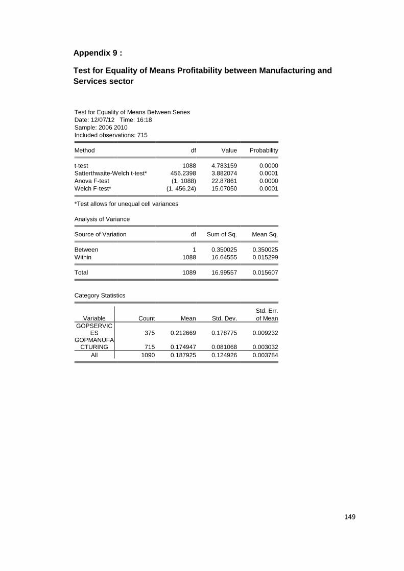
149

Appendix 9 :

Test for Equality of Means Profitability between Manufacturing and

Services sector

Test for Equality of Means Between Series

Date: 12/07/12 Time: 16:18

Sample: 2006 2010

Included observations: 715 Method df Value Probability t-test 1088 4.783159 0.0000

Satterthwaite-Welch t-test* 456.2398 3.882074 0.0001

Anova F-test (1, 1088) 22.87861 0.0000

Welch F-test* (1, 456.24) 15.07050 0.0001 *Test allows for unequal cell variances

Analysis of Variance Source of Variation df Sum of Sq. Mean Sq. Between 1 0.350025 0.350025

Within 1088 16.64555 0.015299 Total 1089 16.99557 0.015607

Category Statistics Std. Err.

Variable Count Mean Std. Dev. of Mean

GOPSERVICES 375 0.212669 0.178775 0.009232

GOPMANUFACTURING 715 0.174947 0.081068 0.003032

All 1090 0.187925 0.124926 0.003784