THE FRISCO CITY SANDSTONE, NORTH FRISCO CITY (PARAMOUNT)

FIELD, MONROE COUNTY, ALABAMA: A CASE STUDY OF NET PAY AND

PERMEABILITY ANISOTROPY EVALUATION RELATED TO GEOLOGY

A Thesis

by

JANICE YVONNE MENKE

Submitted to the Office of Graduate Studies of Texas A&M University

in partial fulfillment of the requirements for the degree of

MASTER OF SCIENCE

May 2002

Major Subject: Petroleum Engineering

THE FRISCO CITY SANDSTONE, NORTH FRISCO CITY (PARAMOUNT)

FIELD, MONROE COUNTY, ALABAMA: A CASE STUDY OF NET PAY AND

PERMEABILITY ANISOTROPY EVALUATION RELATED TO GEOLOGY

A Thesis

by

JANICE YVONNE MENKE

Submitted to the Office of Graduate Studies of Texas A&M University

in partial fulfillment of the requirements for the degree of

MASTER OF SCIENCE

Approved as to style and content by:

Thomas A. Blasingame (Co-Chair of Committee)

Robert R. Berg (Member)

Ronald J. Robinson (Head of Department)

Jerry L. Jensen (Co-Chair of Committee)

Julian E. Gaspar (Member)

May 2002

Major Subject: Petroleum Engineering

ABSTRACT

The Frisco City Sandstone, North Frisco City (Paramount) Field, Monroe County, Alabama:

A Case Study of Net Pay and Permeability Anisotropy Evaluation Related to Geology.

(May 2002)

Janice Yvonne Menke, B.S., Anton de Kom University of Suriname

Co-Chairs of Advisory Committee: Dr. Thomas Blasingame Dr. Jerry Jensen

Net pay and permeability anisotropy are important parameters when making hydrocarbon

reserves estimates. This research focused on the exploration of methods for estimating the net

pay and permeability anisotropy of a heterogeneous hydrocarbon reservoir. I measured the

permeability of two cored intervals of the McCall 25-9 well, located in the North Frisco City

sandstone, Paramount field, Monroe County, Alabama, with a probe permeameter. To compare

and contrast net-pay and permeability-anisotropy evaluations, and to assess the effect of

measurement type and sampling strategy on the results, I used probe, core-plug, and log data.

The permeability anisotropy of a hydrocarbon reservoir should be considered during the dynamic

net-pay estimation. The ratio of vertical to horizontal permeability in a heterogeneous reservoir

is very important since thin, low-permeability layers, which can form a barrier to vertical flow,

may be present. The production forecast may be too optimistic if these layers are not taken into

consideration. The net-pay variation depends on the measurement type. The probe measurements

used here represent the heterogeneity of the reservoir better than core-plug and log

measurements. A reduction in the sampling size did not really affect the probe, core-plug, or log

measurements.

For the net-pay and permeability-anisotropy evaluation of a hydrocarbon reservoir, the probe

permeameter can be an inexpensive, useful device. Measurements can be taken without

destruction of the core samples in a timely and cost-effective manner. In addition, this research

indicated that the probe permeameter can detect thin, low-permeability intervals that usually

cannot be detected during routine analysis of core plugs or log data.

ii

ACKNOWLEDGEMENTS

I wish to express my sincere gratitude and appreciation to the following people:

Dr. Jerry Jensen, co-chair of the advisory committee, for devoting his time to guide me through

my research and correcting my thesis.

Dr. Thomas Blasingame, co-chair of the advisory committee, for always being there whenever I

needed advice or somebody to speak to.

Dr. Robert Berg and Dr. Julian Gaspar for serving as advisory committee members.

Dr. Walter Ayers, for providing me with background information on my research topic.

Patricia Jasse, for being a wonderful and loyal friend.

All my other friends from all over the world for making my study here at Texas A&M

University an unforgettable experience.

Robert Menke, for his never-ending support in every possible way.

And last but not least, my parents, Dorothy & Nizaar, for their support, motivation and trust all

these years.

iii

TABLE OF CONTENTS

Page

ABSTRACT .......................................................................................................................i

ACKNOWLEDGEMENTS.............................................................................................ii

TABLE OF CONTENTS............................................................................................... iii

LIST OF FIGURES ........................................................................................................vi

LIST OF TABLES ..........................................................................................................ix

CHAPTER I .....................................................................................1INTRODUCTION

1.1 Study Objective and Procedures .......................................................................................... 1 1.2 Net Pay................................................................................................................................. 1

1.2.1 Net-Pay Definitions ...................................................................................................... 1 1.2.2 Uses of Net Pay............................................................................................................. 3 1.2.3 Net-Pay Evaluation ....................................................................................................... 4 1.2.4 Problems in Net-Pay Evaluation................................................................................... 7 1.3.1 Permeability Anisotropy Definitions .......................................................................... 10 1.3.2 Uses of Permeability Anisotropy ................................................................................ 10 1.3.3 Permeability Anisotropy Evaluation........................................................................... 12

1.4 The Relationship Between Net Pay and Permeability Anisotropy..................................... 16 1.5 This Study .......................................................................................................................... 17

CHAPTER II GEOLOGICAL SETTING...................................................................18

2.1 Depositional Environment and Reservoir Facies ............................................................... 18 2.2 Reservoir Characterization................................................................................................. 19 2.3 Available Data.................................................................................................................... 21

CHAPTER III DATA COLLECTION ........................................................................24

3.1 Probe Permeameter ............................................................................................................ 24 3.1.1 Probe Measurement Procedure ................................................................................... 25

iv

3.1.1.1 Sampling.............................................................................................................. 25 Page

3.1.1.2 Sample preparation.............................................................................................. 26 3.1.2 Probe Data Acquisition ............................................................................................... 26 3.1.3 Problems and Limitations of Probe Permeametry ...................................................... 26 3.1.4 Probe Measurements on McCall 25-9 Core................................................................ 27

3.2 Core Plugs .......................................................................................................................... 27 3.2.1 Measurement Procedure ............................................................................................. 28

3.2.1.1 Sampling.............................................................................................................. 28 3.2.2 Data Acquisition ......................................................................................................... 28 3.2.3 Problems and Limitations of Core Plugs .................................................................... 29 3.2.4 Plug Data for McCall 25-9.......................................................................................... 30

3.3 Core Plugs versus Probe Permeametry .............................................................................. 30 3.4 Log Data............................................................................................................................. 31

3.4.1 Measurement Procedure ............................................................................................. 31 3.4.2 Data Acquisition ......................................................................................................... 32 3.4.3 Problems and Limitations of Well Logs ..................................................................... 32 3.4.4 Log Data for McCall 25-9 .......................................................................................... 32

3.5 Core-Plug versus Log Data ................................................................................................ 33

CHAPTER IV DATA ANALYSIS ...............................................................................34

4.1 Investigation of the Frisco City Sandstone ........................................................................ 34 4.2 Lithological Assessment of the Core ................................................................................. 34 4.3 Data Comparison................................................................................................................ 36

4.3.1 Analysis of the Effect of Different Probe Seal Sizes and the Lithology..................... 36 4.3.2 Comparison of Probe, Core-Plug, and Log Data ........................................................ 40

4.4 Net Pay Analysis ................................................................................................................ 44 4.4.1 Analysis of Probe Data ............................................................................................... 44

4.4.1.1 Using All Measurements ..................................................................................... 44 4.4.1.2 The Effect of Sample Numbers ........................................................................... 45

4.4.2 Analysis of Core-Plug Data ........................................................................................ 49 4.4.2.1 Using All Measurements ..................................................................................... 49 4.4.2.2 The Effect of Sample Numbers ........................................................................... 50

4.4.3 Analysis of Log Data .................................................................................................. 53 4.4.3.1 Using All Measurements ..................................................................................... 53 4.4.3.2 The Effect of Sample Numbers ........................................................................... 53

4.4.4 Comparison of Probe, Core-Plug and Log Net Pay Estimates ................................... 56 4.4.5 Comparison of Core-Plug and Log Data for the Entire Interval................................. 60 4.4.6 Estimated N/G Ratio for the Frisco City Sandstone ................................................... 61

4.5 Further Analysis of Probe and Core-Plug Data.................................................................. 62 4.5.1 Probe Permeability Averages...................................................................................... 62 4.5.2 Probe Permeability Variabilities ................................................................................. 64 4.5.3 Core-Plug Averages.................................................................................................... 65 4.5.4 Comparison of Probe and Core-Plug Statistics........................................................... 66 4.5.5 Correlation .................................................................................................................. 66

v

4.5.5.1 Linear Correlation ............................................................................................... 66 Page

4.5.5.2 Log-Transformed Permeability Correlation ........................................................ 69 4.5.6 Lorenz curves.............................................................................................................. 70

4.6 Results and Implications for Other Reservoirs .................................................................. 72

CHAPTER V SUMMARY ............................................................................................74

5.1 Conclusions ........................................................................................................................ 74 5.1.1 Conclusions Resulting from Literature Survey........................................................... 74

5.1.2 Conclusions Specific to the Frisco City Sandstone......................................................... 75 5.2 General Observations ......................................................................................................... 76 5.3 Suggestions for Further Work ............................................................................................ 77

NOMENCLATURE .......................................................................................................78

REFERENCES ...............................................................................................................79

APPENDIX A EQUATIONS ........................................................................................83

APPENDIX B GEOLOGICAL DESCRIPTION OF CORED INTERVALS..........85

VITA................................................................................................................................87

vi

LIST OF FIGURES

................................................................................................................................... Page

Fig. 1.1 - Differences in net pay depend on its usage..................................................................... 4 Fig. 1.2 - Coregraph method .......................................................................................................... 6 Fig. 1.3 - Two sand layers in a hydrocarbon reservoir seem to have the same thickness but have different net pays. ................................................................................................... 8 Fig. 1.4 - Net pay differs among wells within the same sand body................................................ 9 Fig. 1.5 - Thin shale barriers reduce net pay in hydrocarbon reservoirs. ..................................... 11 Fig. 1.6 - Unfavorable permeability distribution reduces the effect of waterflooding. ................ 11 Fig. 1.7 - Favorable permeability distribution leads to successful waterflooding........................ 12 Fig. 1.8 - Horizontal and vertical core-plug sampling ................................................................. 13 Fig. 1.9 - Three main sandstone reservoir types . ......................................................................... 16 Fig. 2.1 - Frisco City sandstone ................................................................................................... 19 Fig. 2.2 - Areas of the Frisco City sandstone development, southern Alabama .......................... 20 Fig. 2.3 - Composite core description for the Frisco City sandstone, Monroe County, Alabama, showing facies types, lithology, and sedimentary structures ....................... 22 Fig. 2.4 - Dataset 1 core-plug permeability and porosity.. ........................................................... 23 Fig. 2.5 - Dataset 2 core-plug permeability and porosity ............................................................. 23 Fig. 3.1 - Schematic representation of a probe permeameter. ...................................................... 25 Fig. 3.2 - A Hassler sleeve used to measure core-plug permeability............................................ 29 Fig. 3.3 - Difference in values between probe and core-plug permeability at the same depth .... 31 Fig. 4.1 - Assessment of the lithological behavior of Dataset 1 with depth. ................................ 35 Fig. 4.2 - Assessment of the lithological behavior of Dataset 2 with depth. ................................ 35 Fig. 4.3 - Assessment of the effect of different tip sizes and their relation to the lithology......... 36

vii

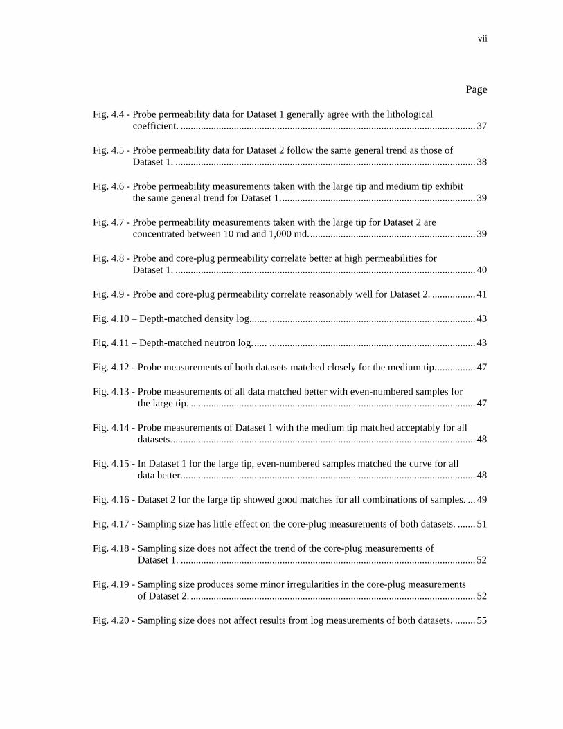
Page Fig. 4.4 - Probe permeability data for Dataset 1 generally agree with the lithological coefficient. .................................................................................................................... 37 Fig. 4.5 - Probe permeability data for Dataset 2 follow the same general trend as those of Dataset 1. ...................................................................................................................... 38 Fig. 4.6 - Probe permeability measurements taken with the large tip and medium tip exhibit the same general trend for Dataset 1............................................................................. 39 Fig. 4.7 - Probe permeability measurements taken with the large tip for Dataset 2 are concentrated between 10 md and 1,000 md.................................................................. 39 Fig. 4.8 - Probe and core-plug permeability correlate better at high permeabilities for Dataset 1. ...................................................................................................................... 40 Fig. 4.9 - Probe and core-plug permeability correlate reasonably well for Dataset 2. ................. 41 Fig. 4.10 – Depth-matched density log....... ................................................................................. 43 Fig. 4.11 – Depth-matched neutron log...... ................................................................................. 43 Fig. 4.12 - Probe measurements of both datasets matched closely for the medium tip................ 47 Fig. 4.13 - Probe measurements of all data matched better with even-numbered samples for the large tip. ................................................................................................................ 47 Fig. 4.14 - Probe measurements of Dataset 1 with the medium tip matched acceptably for all datasets........................................................................................................................ 48 Fig. 4.15 - In Dataset 1 for the large tip, even-numbered samples matched the curve for all data better.................................................................................................................... 48 Fig. 4.16 - Dataset 2 for the large tip showed good matches for all combinations of samples. ... 49 Fig. 4.17 - Sampling size has little effect on the core-plug measurements of both datasets. ....... 51 Fig. 4.18 - Sampling size does not affect the trend of the core-plug measurements of Dataset 1. .................................................................................................................... 52 Fig. 4.19 - Sampling size produces some minor irregularities in the core-plug measurements of Dataset 2. ................................................................................................................ 52 Fig. 4.20 - Sampling size does not affect results from log measurements of both datasets. ........ 55

viii

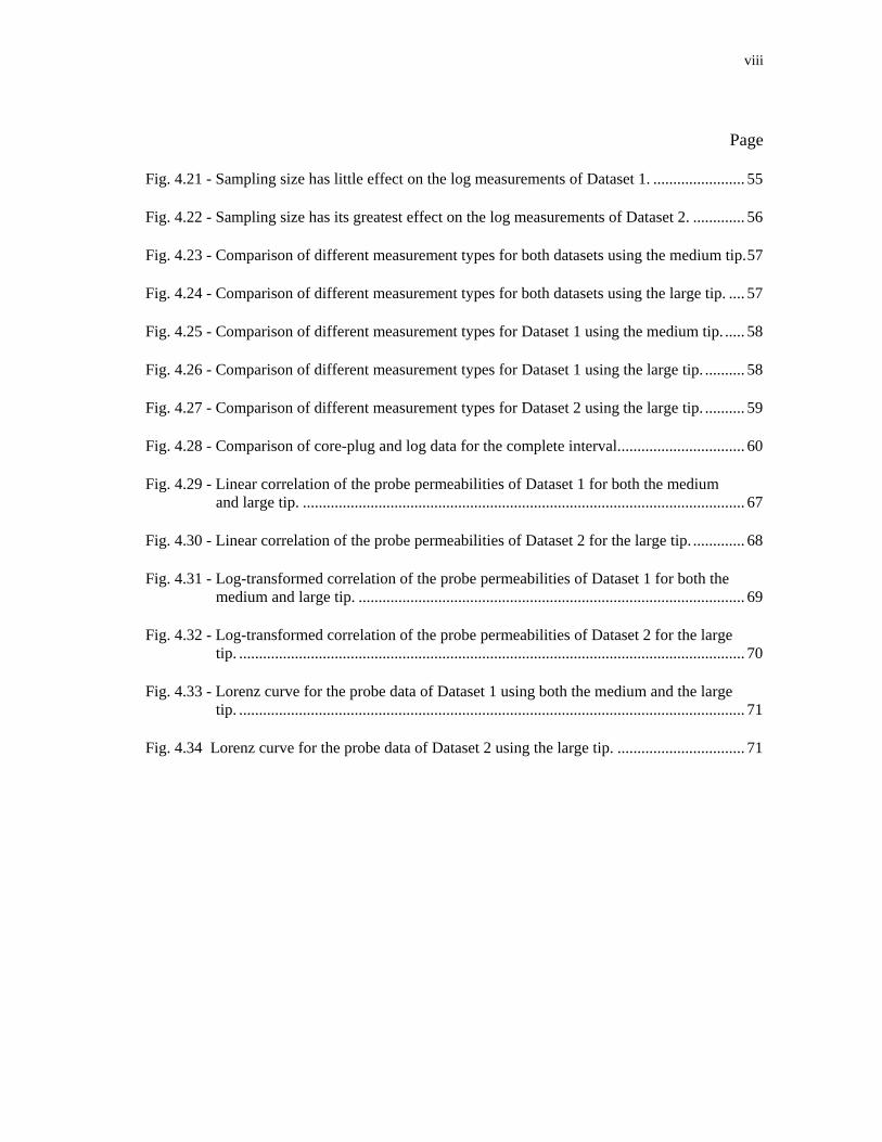
Page Fig. 4.21 - Sampling size has little effect on the log measurements of Dataset 1. ....................... 55 Fig. 4.22 - Sampling size has its greatest effect on the log measurements of Dataset 2. ............. 56 Fig. 4.23 - Comparison of different measurement types for both datasets using the medium tip.57 Fig. 4.24 - Comparison of different measurement types for both datasets using the large tip. .... 57 Fig. 4.25 - Comparison of different measurement types for Dataset 1 using the medium tip. ..... 58 Fig. 4.26 - Comparison of different measurement types for Dataset 1 using the large tip. .......... 58 Fig. 4.27 - Comparison of different measurement types for Dataset 2 using the large tip. .......... 59 Fig. 4.28 - Comparison of core-plug and log data for the complete interval................................ 60 Fig. 4.29 - Linear correlation of the probe permeabilities of Dataset 1 for both the medium and large tip. ............................................................................................................... 67 Fig. 4.30 - Linear correlation of the probe permeabilities of Dataset 2 for the large tip. ............. 68 Fig. 4.31 - Log-transformed correlation of the probe permeabilities of Dataset 1 for both the medium and large tip. ................................................................................................. 69 Fig. 4.32 - Log-transformed correlation of the probe permeabilities of Dataset 2 for the large tip. ............................................................................................................................... 70 Fig. 4.33 - Lorenz curve for the probe data of Dataset 1 using both the medium and the large tip. ............................................................................................................................... 71 Fig. 4.34 Lorenz curve for the probe data of Dataset 2 using the large tip. ................................ 71

ix

LIST OF TABLES

Page

TABLE 4.1 RESULTS OF THE NET PAY ANALYSIS USING ALL PROBE MEASUREMENTS... 44

TABLE 4.2 RESULTS OF THE NET PAY ANALYSIS USING THE UNEVEN NUMBER OF PROBE SAMPLES. ............................................................................................................. 45 TABLE 4.3 RESULTS OF THE NET PAY ANALYSIS USING THE EVEN NUMBER OF PROBE SAMPLES. .......................................................................................................................... 46

TABLE 4.4 RESULTS OF THE NET PAY ANALYSIS USING ALL CORE-PLUG MEASUREMENTS............................................................................................................. 50

TABLE 4.5 RESULTS OF THE NET PAY ANALYSIS USING UNEVEN CORE-PLUG MEASUREMENTS............................................................................................................. 50

TABLE 4.6 RESULTS OF THE NET PAY ANALYSIS USING EVEN CORE-PLUG MEASUREMENTS............................................................................................................. 50

TABLE 4.7 RESULTS OF THE NET PAY ANALYSIS USING LOG MEASUREMENTS................ 53

TABLE 4.8 RESULTS OF THE NET PAY ANALYSIS USING UNEVEN LOG MEASUREMENTS............................................................................................................. 54

TABLE 4.9 RESULTS OF THE NET PAY ANALYSIS USING EVEN CORE-PLUG MEASUREMENTS............................................................................................................. 54

TABLE 4.10 N/G RATIOS FOR THE DIFFERENT MEASUREMENT TYPES FOR A PERMEABILITY CUTOFF OF 1 MD. ............................................................................... 61

TABLE 4.11 AVERAGES FOR DATASET 1 USING THE LARGE AND MEDIUM TIP.................... 63

TABLE 4.12 AVERAGES FOR DATASET 2 USING THE LARGE TIP. .............................................. 63

TABLE 4.13 AVERAGES FOR BOTH DATASETS OF THE CORE-PLUG DATA............................. 66

1

CHAPTER I

INTRODUCTION

1.1 Study Objective and Procedures

This research project explores methods for estimating the net pay and the permeability

anisotropy of a heterogeneous hydrocarbon reservoir. To achieve this objective, I performed the

following studies:

• Evaluated several methods of estimating net pay and permeability anisotropy.

• Compared and contrasted these evaluations in the Frisco City sandstone formation.

• Assessed the effect of the sampling strategy on the results.

• Assessed the effect of the measurement type on the results.

• Evaluated the response of the different measurement types to geological variation.

1.2 Net Pay

To forecast the performance of hydrocarbon reservoirs, an accurate estimation of net pay is often

necessary. Producible net pay is that part of the formation consisting of reservoir quality rock.1 It

is an important parameter for several reservoir evaluation procedures, including the estimation of

the volumetric hydrocarbons in place (reserve estimate), well-test interpretations, and reservoir

productivity.2

1.2.1 Net-Pay Definitions

Although net pay would appear to be a straightforward reservoir characteristic, its definition and

evaluation have a number of subtleties. Despite many years of use of these concepts, no distinct,

This thesis follows the style of the SPE Reservoir Evaluation and Engineering.

2

unambiguous definition has been established and therefore each case has to be treated

individually. Several authors, such as Cobb and Marek2, Calhoun3,Pirson4, and Snyder5, have

discussed net-pay definitions. Indeed, SPE recently (August 2000) convened a meeting to

discuss the definition of net pay.

Net-pay definitions may be classified as either static or dynamic. Starting with the static

definitions, which do not involve fluid flow in the reservoir, Cobb and Marek2 defined net pay as

“that part of the reservoir containing hydrocarbons that can be recovered economically.”

Calhoun3 defines it as “that portion of the reservoir believed to be commercially productive.”

Both definitions take the economic aspect into account. However, these definitions do not

include porosity and permeability, which are very important parameters used to calculate the

recoverable reserves. Calhoun’s definition does not mention hydrocarbons at all, and could as

well be used for water production.

The dynamic definitions of net pay involve the ability of the reservoir to permit fluid flow.

Pirson4 defines net pay in his textbook as “that part of the reservoir thickness, which contributes

to oil recovery and is defined by lower limits of porosity and permeability and upper limits of

water saturation.” Snyder5 states that net pay is that part of the reservoir that contains

hydrocarbons and is both porous and permeable. Both definitions take the porosity and

permeability into account, but Snyder’s definition does not include the water saturation.

We usually express net pay in terms of thickness, a one-dimensional feature. This is based on the

simpler (static) view, where fluids are not required to move. The dynamic form of net pay may

involve connectivity and, therefore, could have a three-dimensional aspect. This would make net

pay more difficult to define and apply.

Net pay consists only of the net effective zone. This is in contrast to gross pay, which also

includes the non reservoir-quality rocks such as shales.6 For static net pay, the presence of shales

simply subtracts from the gross-pay thickness, because the flow of fluids is not involved in this

definition. However, when defining dynamic net pay, the effects of shales can be much more

complex because even thin shales can be significant barriers to fluid flow.

3

Gaynor and Sneider7 suggest the use of capillary analysis (mercury injection) to determine net

pay. It is possible to predict the rock/fluid system behavior because the hydrocarbon

displacement depends on the pore-throat geometry, fluid saturations, and the fluid properties of

immiscible wetting and non wetting phases. After the identification of reservoir quality rock, net

pay can be determined by applying the appropriate cutoff values.

1.2.2 Uses of Net Pay

Net pay can be determined and used for several purposes. Some of the uses involve static

aspects, while others use dynamic aspects of the reservoir. The uses that require static net pay

include:

• Determining Hydrocarbon Content

This quantitative determination uses net pay for the calculation of the amount of

hydrocarbons present in a reservoir. This may include both movable and non-

movable hydrocarbons.5

• Net-Pay Isopach Maps

Net-pay isopach maps can be used as a guide for development drilling and design

and installation of secondary recovery projects.1 This method is a more

qualitative application.

Dynamic net pay is used for:

• Areal Sweep

For the evaluation of waterflood project economics, the net pay has to be

calculated to determine the area of the reservoir with relative permeability

favorable to fluid injection. Areal sweep is optimal when the direction of

maximum permeability is parallel to the line connecting injection wells in the

vicinity.8

• Well Testing

The major purpose of well testing is to determine the ability of a formation to

produce reservoir fluids. Reservoir boundaries must be defined and therefore the

net effective flowing interval has to be determined.9

4

• Well Placement

It is important to place wells in areas with the largest net pay to be assured of

high productivity and optimum hydrocarbon production.

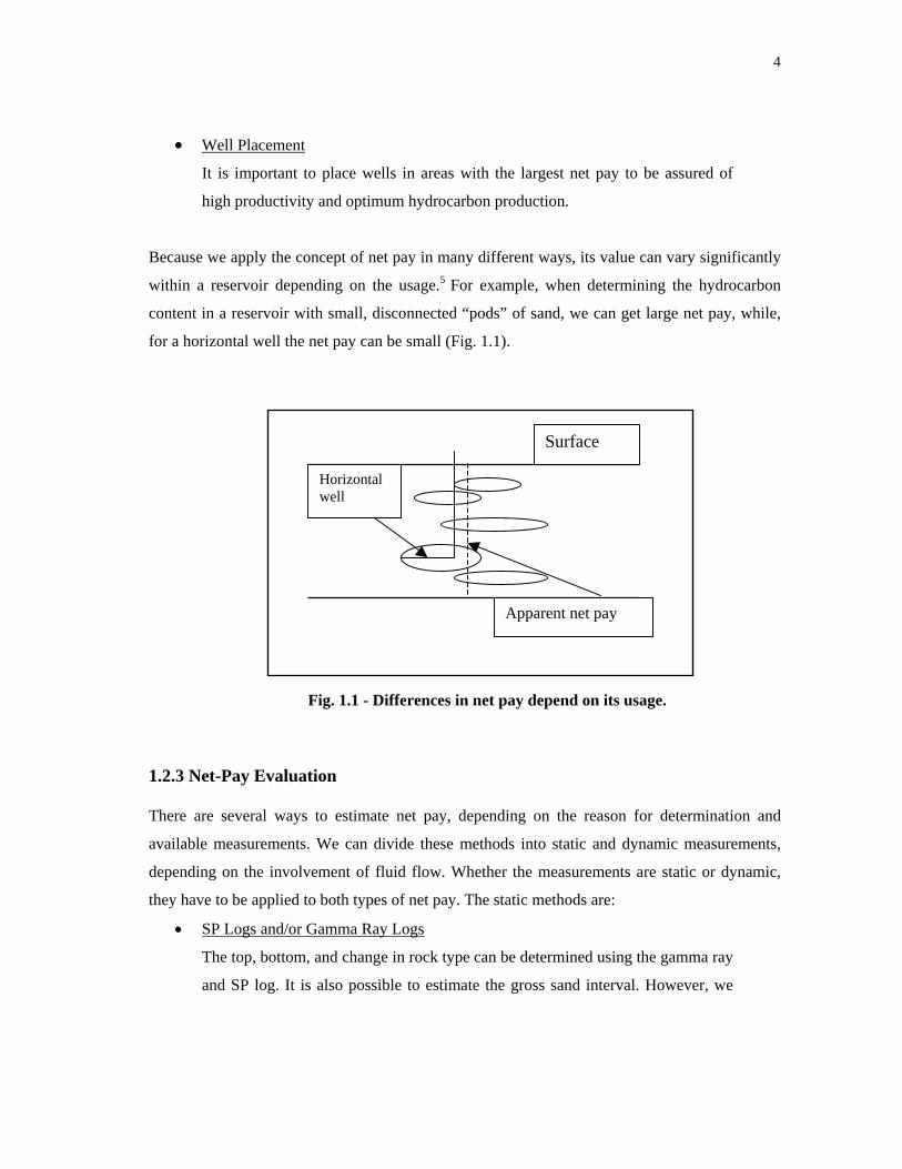
Because we apply the concept of net pay in many different ways, its value can vary significantly

within a reservoir depending on the usage.5 For example, when determining the hydrocarbon

content in a reservoir with small, disconnected “pods” of sand, we can get large net pay, while,

for a horizontal well the net pay can be small (Fig. 1.1).

Apparent net pay

Surface

Horizontal well

Fig. 1.1 - Differences in net pay depend on its usage. 1.2.3 Net-Pay Evaluation

There are several ways to estimate net pay, depending on the reason for determination and

available measurements. We can divide these methods into static and dynamic measurements,

depending on the involvement of fluid flow. Whether the measurements are static or dynamic,

they have to be applied to both types of net pay. The static methods are:

• SP Logs and/or Gamma Ray Logs

The top, bottom, and change in rock type can be determined using the gamma ray

and SP log. It is also possible to estimate the gross sand interval. However, we

5

only apply this method if alternating clean, permeable, and porous sandstone and

shale form the stratigraphic sequence.

• Porosity Logs Combined With SP and Gamma Ray Logs

After defining the gross sand thickness, we can determine the porous interval

using a lower limit or porosity cutoff by combining porosity logs with SP and

gamma ray logs. This method has the same limitations as the previous one.

• Isopach or Isochore Maps

Isopach and isochore maps represent either the true stratigraphic thickness or the

total aggregate vertical thickness of porous reservoir quality rock in a 3D view.1

• Micrologs

The methods mentioned above may not detect thin, impermeable beds such as

shales, resulting in an overestimation of net pay. Conversely, thin, permeable

intervals can be missed, causing an underestimation of net pay. The microlog is a

crude but high-resolution resistivity measurement that responds to the presence

of the mud cake and may identify permeable intervals.10

Any of the methods above might not discriminate between hydrocarbon-bearing intervals and

water-bearing intervals.

The dynamic methods that involve fluid flow also include permeability. To define the net pay, a

permeability cut off is often used that depends on the fluid viscosity, permeability distribution,

reservoir-pressure differentials, and reservoir-drive mechanism.2

• Core Analysis and Core Description With Porosity, Resistivity, SP and Gamma

Ray Logs

In core analysis and description, we use permeability and oil-saturation data to

estimate net pay. The oil saturation is determined from resistivity logs. Core

analysis and core description are used to estimate the oil saturation in reservoirs

with long transition zones. The total gross sand interval is determined using SP

and gamma ray logs. The porosity logs are used to determine the formation

porosity. After permeability cutoff values are defined, they are correlated with

porosity cutoff values. In addition, we determine the oil/water contact to estimate

the total oil content of the reservoir.5

6

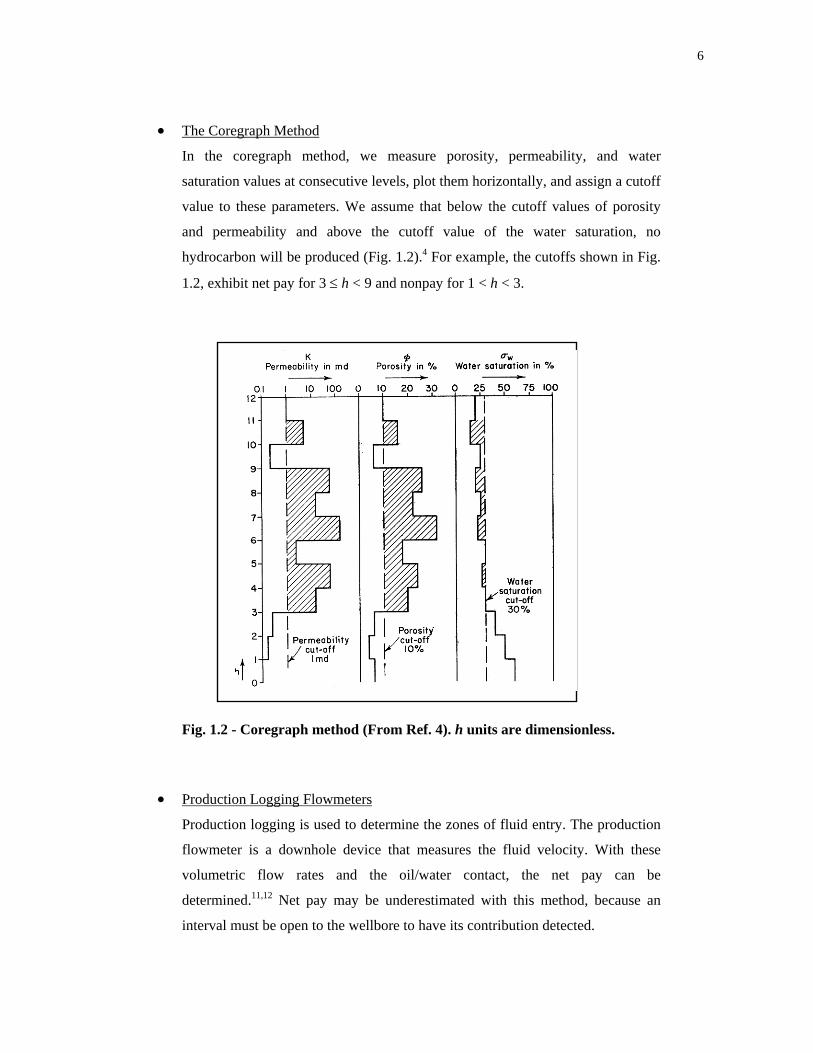
• The Coregraph Method

In the coregraph method, we measure porosity, permeability, and water

saturation values at consecutive levels, plot them horizontally, and assign a cutoff

value to these parameters. We assume that below the cutoff values of porosity

and permeability and above the cutoff value of the water saturation, no

hydrocarbon will be produced (Fig. 1.2).4 For example, the cutoffs shown in Fig.

1.2, exhibit net pay for 3 ≤ h < 9 and nonpay for 1 < h < 3.

Fig. 1.2 - Coregraph method (From Ref. 4). h units are dimensionless.

• Production Logging Flowmeters

Production logging is used to determine the zones of fluid entry. The production

flowmeter is a downhole device that measures the fluid velocity. With these

volumetric flow rates and the oil/water contact, the net pay can be

determined.11,12 Net pay may be underestimated with this method, because an

interval must be open to the wellbore to have its contribution detected.

7

• Formation Testers

During the operation of a wireline formation test device, reservoir fluids flow

into the tool. We can determine net pay with the amount of fluid present in the

tool and the drawdown and buildup pressures.13

1.2.4 Problems in Net-Pay Evaluation

A variety of issues complicate net-pay evaluation. Some issues are relatively straightforward,

caused by measurement error or sampling. These include:

• The difference between the air permeability of the reservoir rock and its

permeability to water and oil.5

Usually the air permeability is higher because it assumes only one phase, the

Klinkenberg effect, and the absence of the overlying rock pressure. Therefore,

the estimation of the net-pay thickness will be optimistic.

• From core plugs, only information for cored and sampled intervals can be

derived, since plugs are taken every foot.

The estimation of net pay can be either optimistic or pessimistic, depending on

the core-plug value of a particular reservoir property. Core plugs do not

necessarily represent the entire reservoir since they are small samples and are

taken only at the wellbore. In contrast, well logs provide information over a

larger volume and cover the entire logged interval.

The wellbore evaluation of net pay, which may be a 3D property, is not always representative of

the surrounding formation. For example, if a well is drilled in a reservoir with a pay zone

thickness of 20 ft, this layer does not necessarily need to have the same thickness at a lateral

distance 100 ft away from the wellbore. Here, the units of net pay are expressed in terms of

length, but taking into consideration that net pay can be a 3D property, the actual units should be

volumetric.

Nonpay is that part of the reservoir that cannot be produced economically. Often, nonpay is

overlooked because companies are usually only interested in that part of the reservoir that

appears to contribute to economic production. However, nonpay may play an important role in

8

determining net pay. Nonpay may be particularly important for controlling the connectivity

within the sands, affecting the reservoir’s 3D net-pay value and the permeability anisotropy

(vertical-to-horizontal permeability).

A

surface

Well B sand

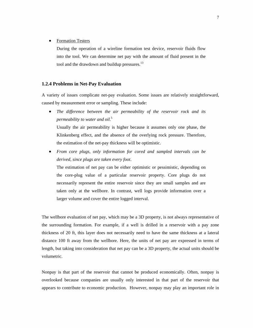
Fig. 1.3 - Two but have differ

In Fig. 1.3 the two s

even though there is

because the sand bod

The hydrocarbon pr

among wells. Discon

in sedimentary rocks

For example, a sand

Usually sands becom

and therefore the net

Wells B and C can b

the fault is present.

Well

sand layers in a hydrocarbon reservoir seem to have the same thickness ent net pays.

and bodies seem to have the same thickness when measured at the wells,

no continuity between the layers. However, their net pays are not the same

y in Well A is larger than the sand body in Well B.

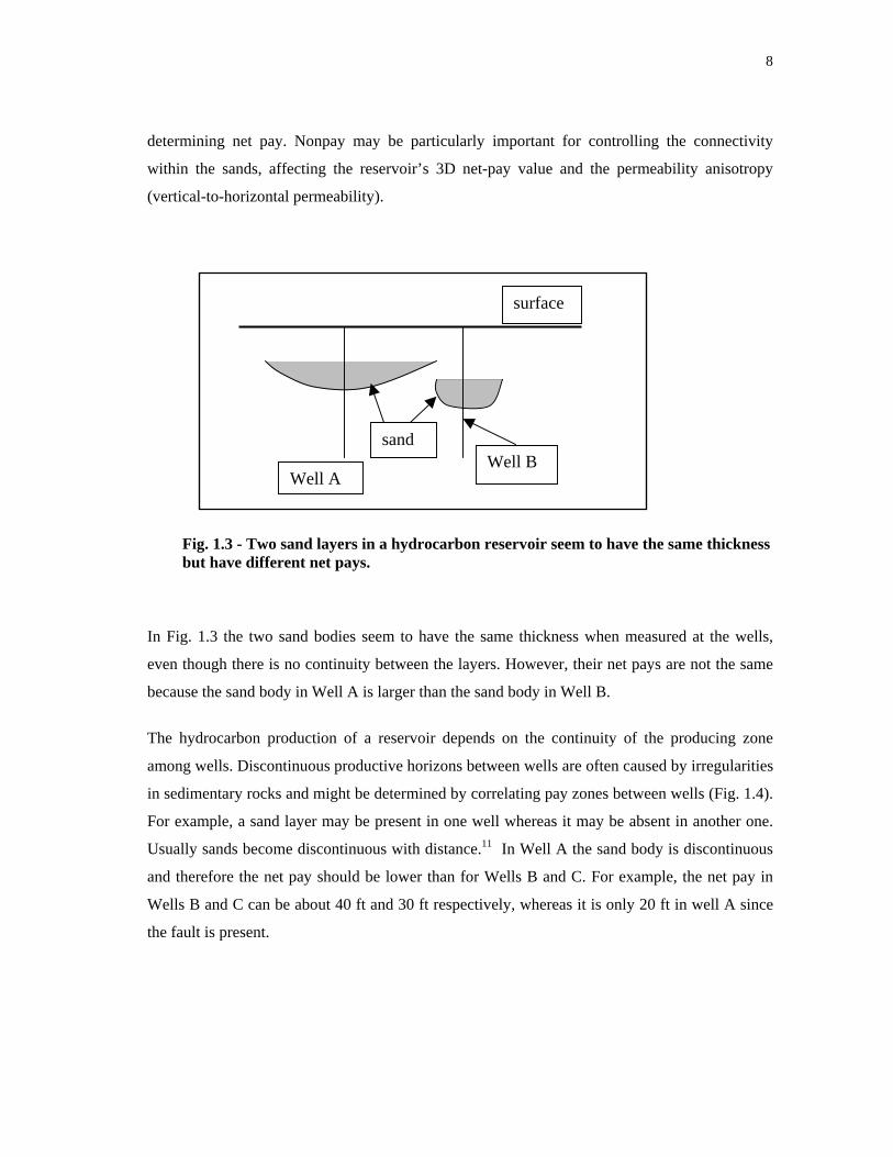
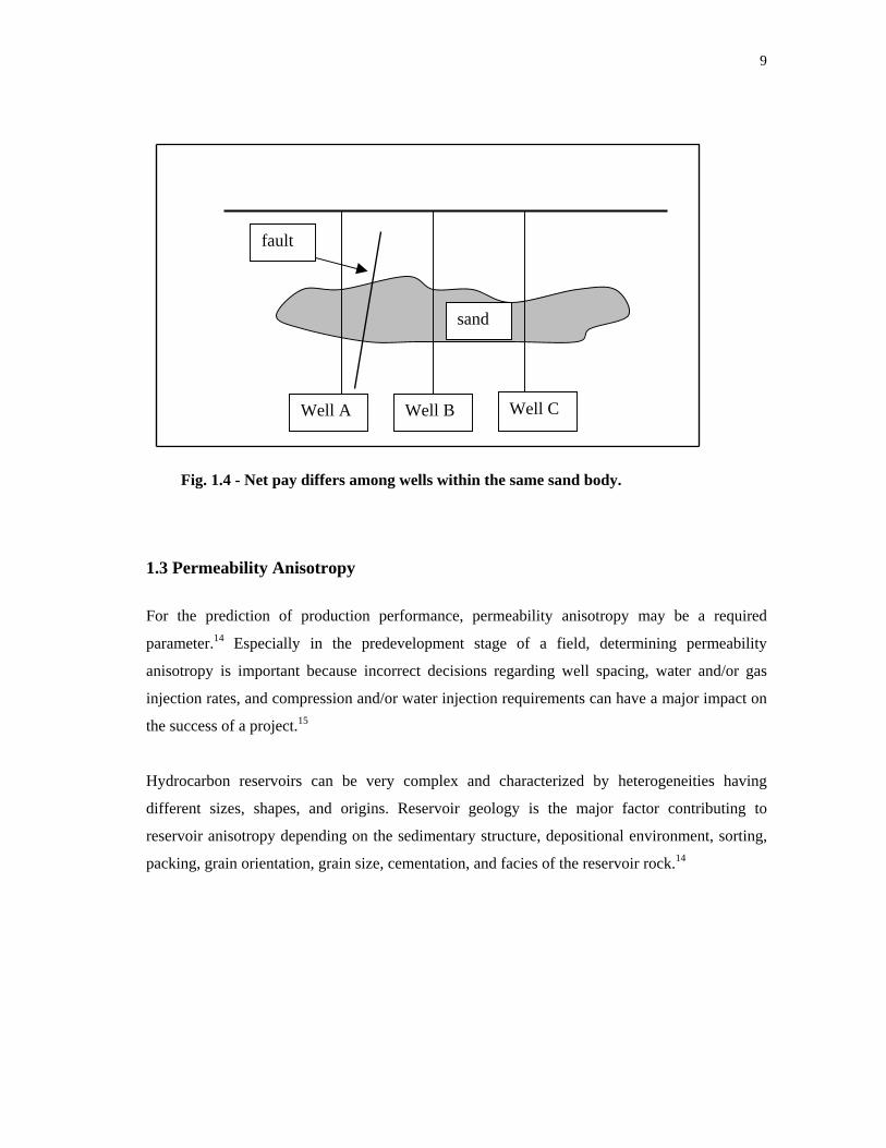
oduction of a reservoir depends on the continuity of the producing zone

tinuous productive horizons between wells are often caused by irregularities

and might be determined by correlating pay zones between wells (Fig. 1.4).

layer may be present in one well whereas it may be absent in another one.

e discontinuous with distance.11 In Well A the sand body is discontinuous

pay should be lower than for Wells B and C. For example, the net pay in

e about 40 ft and 30 ft respectively, whereas it is only 20 ft in well A since

9

sand

Well A Well B Well C

fault

Fig. 1.4 - Net pay differs among wells within the same sand body.

1.3 Permeability Anisotropy

For the prediction of production performance, permeability anisotropy may be a required

parameter.14 Especially in the predevelopment stage of a field, determining permeability

anisotropy is important because incorrect decisions regarding well spacing, water and/or gas

injection rates, and compression and/or water injection requirements can have a major impact on

the success of a project.15

Hydrocarbon reservoirs can be very complex and characterized by heterogeneities having

different sizes, shapes, and origins. Reservoir geology is the major factor contributing to

reservoir anisotropy depending on the sedimentary structure, depositional environment, sorting,

packing, grain orientation, grain size, cementation, and facies of the reservoir rock.14

10

1.3.1 Permeability Anisotropy Definitions

Permeability anisotropy is caused by the difference between the horizontal (kh) and vertical (kv)

permeability. In turn, permeability anisotropy, or the directional dependence of petrophysical

transport properties, causes fluids to flow at different rates and in different directions for a

particular flow potential.14

Schlumberger et al.16 suggested that two types of anisotropy can be distinguished: microscopic

anisotropy, owing to preferred orientation of the rock fabric, and macroscopic anisotropy, caused

by the different properties of sequential, parallel, homogeneous rock layers. However, these

anisotropies do not include heterogeneous rock layers. For example, with crossbedding,

involving the alternate layering of sands with different properties at an angle with the

depositional features, these two categories do not apply.17

1.3.2 Uses of Permeability Anisotropy

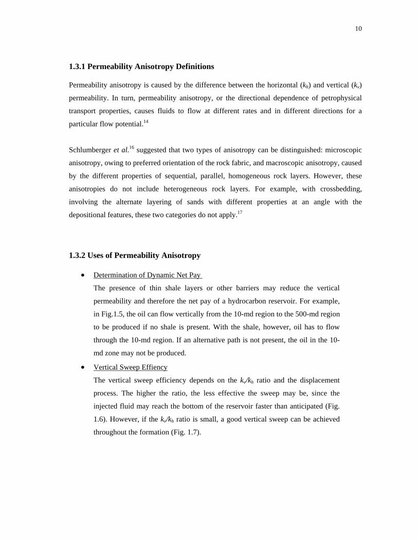
• Determination of Dynamic Net Pay

The presence of thin shale layers or other barriers may reduce the vertical

permeability and therefore the net pay of a hydrocarbon reservoir. For example,

in Fig.1.5, the oil can flow vertically from the 10-md region to the 500-md region

to be produced if no shale is present. With the shale, however, oil has to flow

through the 10-md region. If an alternative path is not present, the oil in the 10-

md zone may not be produced.

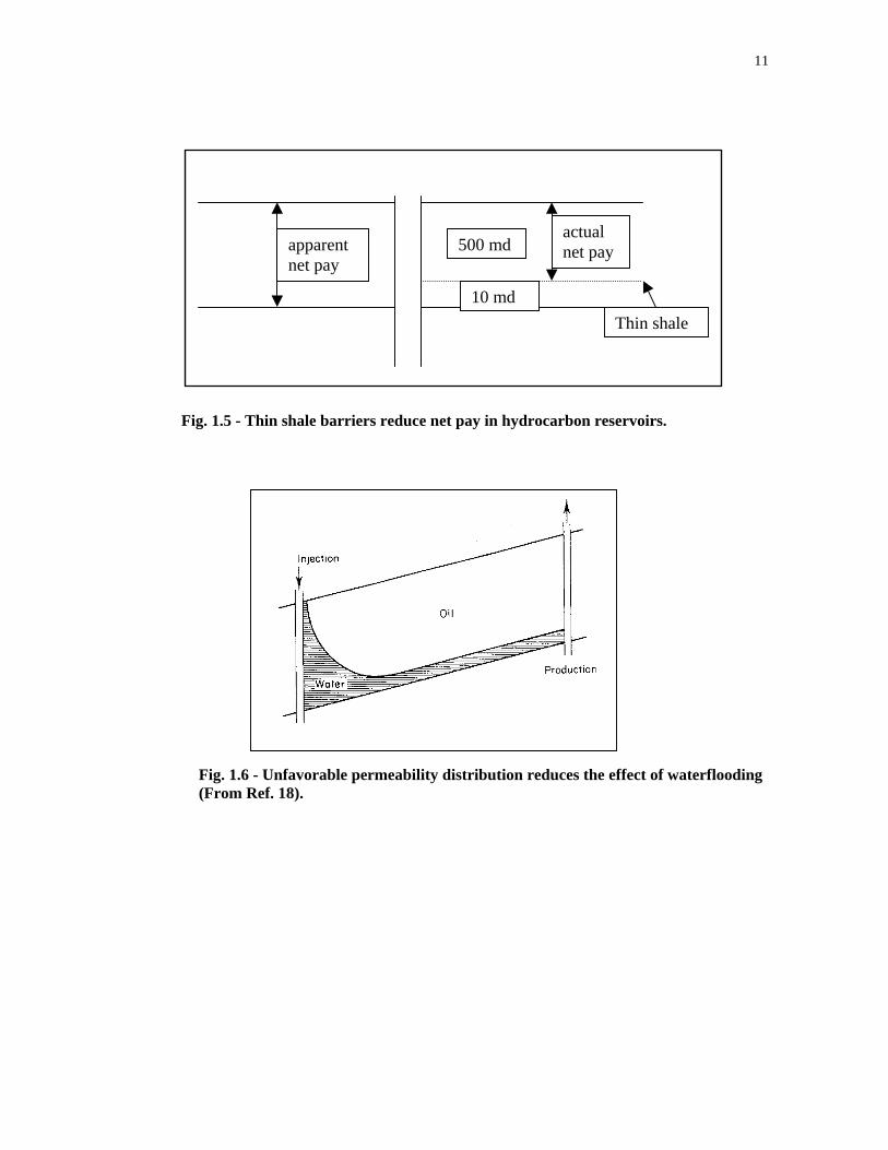
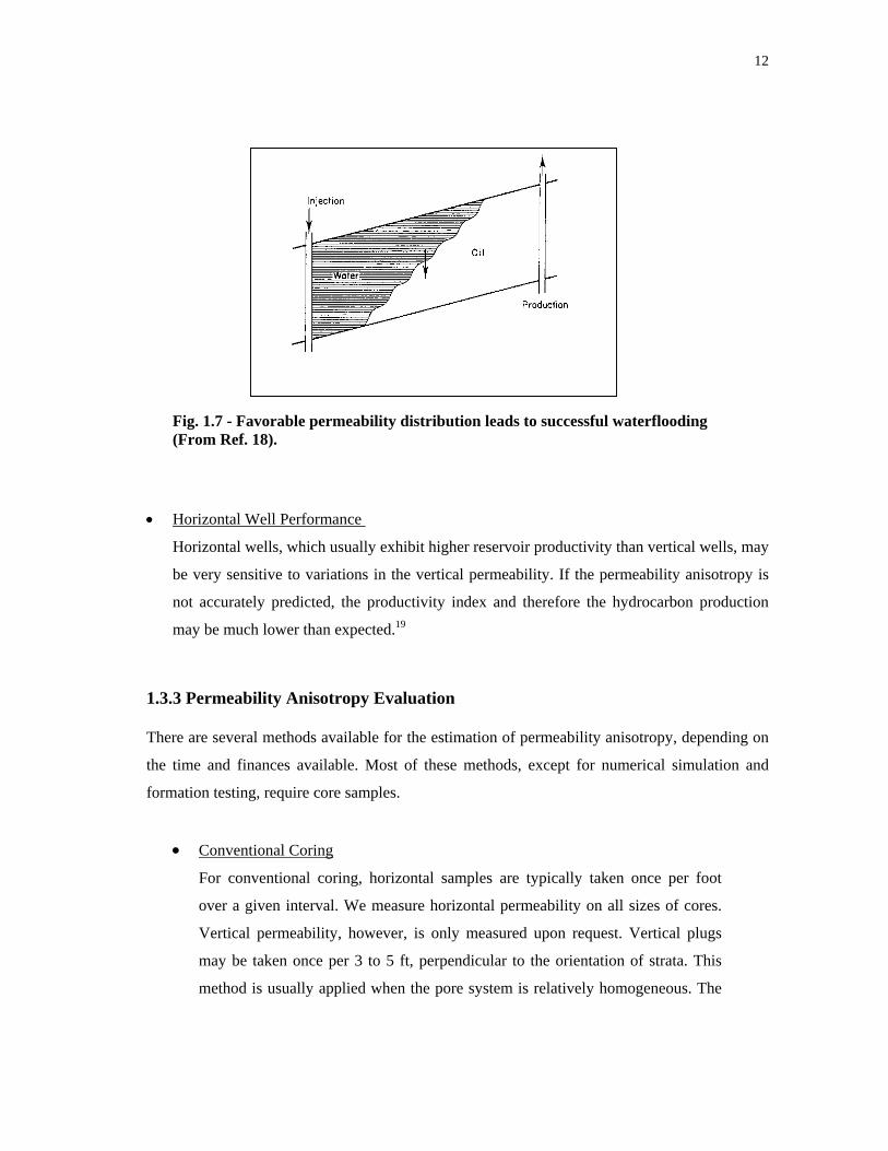
• Vertical Sweep Effiency

The vertical sweep efficiency depends on the kv/kh ratio and the displacement

process. The higher the ratio, the less effective the sweep may be, since the

injected fluid may reach the bottom of the reservoir faster than anticipated (Fig.

1.6). However, if the kv/kh ratio is small, a good vertical sweep can be achieved

throughout the formation (Fig. 1.7).

11

Fig. 1.5 - Thin shale barriers reduce net

Fig. 1.6 - Unfavorable permeability d(From Ref. 18).

actual net payapparent

net pay

500 md

p

ist

10 md

ay in hydrocarbon re

ribution reduces the

Thin shale

servoirs.

effect of waterflooding

12

Fig. 1.7 - Favorable permeability distribution leads to successful waterflooding (From Ref. 18).

• Horizontal Well Performance

Horizontal wells, which usually exhibit higher reservoir productivity than vertical wells, may

be very sensitive to variations in the vertical permeability. If the permeability anisotropy is

not accurately predicted, the productivity index and therefore the hydrocarbon production

may be much lower than expected.19

1.3.3 Permeability Anisotropy Evaluation

There are several methods available for the estimation of permeability anisotropy, depending on

the time and finances available. Most of these methods, except for numerical simulation and

formation testing, require core samples.

• Conventional Coring

For conventional coring, horizontal samples are typically taken once per foot

over a given interval. We measure horizontal permeability on all sizes of cores.

Vertical permeability, however, is only measured upon request. Vertical plugs

may be taken once per 3 to 5 ft, perpendicular to the orientation of strata. This

method is usually applied when the pore system is relatively homogeneous. The

13

less homogeneous, the more sampling is required. Core-plug data are used for

permeability estimation, but thin, low-permeability reservoir intervals can be

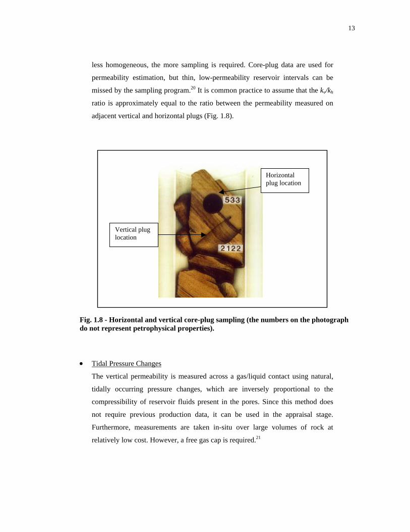
missed by the sampling program.20 It is common practice to assume that the kv/kh

ratio is approximately equal to the ratio between the permeability measured on

adjacent vertical and horizontal plugs (Fig. 1.8).

Vertical plug location

Horizontal plug location

Fig. 1.8 - Horizontal and vertical core-plug sampling (the numbers on the photograph do not represent petrophysical properties). • Tidal Pressure Changes

The vertical permeability is measured across a gas/liquid contact using natural,

tidally occurring pressure changes, which are inversely proportional to the

compressibility of reservoir fluids present in the pores. Since this method does

not require previous production data, it can be used in the appraisal stage.

Furthermore, measurements are taken in-situ over large volumes of rock at

relatively low cost. However, a free gas cap is required.21

14

• Wireline Formation Testers

Wireline formation testers are used to obtain pressure versus depth profiles of

reservoirs by performing a series of point pressure tests.22 The permeability is

calculated with Darcy’s Law.23 With a multiprobe wireline formation tester,

vertical and horizontal mobilities can be determined at specified depths to

provide a profile of permeability anisotropy versus depth. The recorded transient

pressures provide estimates for the horizontal and vertical permeability within the

radius of investigation.22

• Well Logs

There are three ways to determine permeability from wireline logs:

♦ Correlation of core-plug permeability and log measurements.

♦ Magnetic Resonance Imaging Log (MRIL) nuclear magnetic resonance

(NMR) - derived permeabilities.

The NMR signal measures porosity. The pore space’s surface-to-volume

ratio is measured by the rate of decay of the echo amplitudes. The

permeability can be calculated with either the Coates equation23 or the SDR

model24 (Appendix A). The Coates equation uses the ratio of moveable-to-

bound fluid saturation and the porosity, while the SDR model uses the

geometrical mean of the relaxation spectra.

♦ Multiple Array Acoustic (MAC) Stonely wave permeabilities.

The permeability is estimated from the decay or attenuation of the low-

frequency acoustic Stonely waves, which are propagated along the borehole

interface. We use a parameter combination, which controls the permeability-

related Stonely wave attenuation and dispersion.23

The permeability anisotropy is estimated by taking the harmonic average for

the vertical permeability (kv) and the arithmetic average for the horizontal

permeability (kh) and calculating the ratio (kv/kh) of log-derived values.25

However, the log values are not measured in a particular direction and this

may represent a problem when trying to determine the permeability

anisotropy.

15

• Numerical Methods

There are several numerical methods to predict anisotropy.

♦ History Matching Against Field Production

When production data from wells are available, we can use the flow

simulator to predict the kv/kh ratio. However, the predicted value may not be

accurate because of the nonuniqueness of the model.

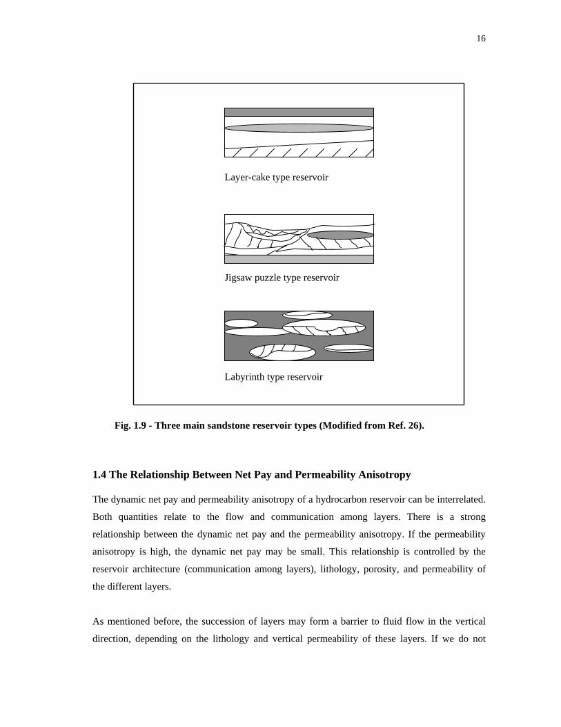
♦ Averages for Layered Systems

Weber and Van Geuns26 distinguished three main sandstone reservoir types

(Fig. 1.9):

Layer-cake reservoirs

Layer-cake reservoirs consist of layers stacked on one another without

major discontinuities in horizontal permeability.

Jigsaw-puzzle reservoirs

Low or nonpermeable layers occasionally interbed jigsaw-puzzle

reservoirs.

Labyrinth reservoirs

Heterogeneous labyrinth reservoirs do not necessarily have to be

discontinuous. In addition, low or nonpermeable layers interbed them,

and the succession of layers is very complex.

If the flow within strata is lateral (layer-cake reservoir), we use the arithmetic average. If

we want to include the vertical flow, especially for jigsaw-structured reservoirs, we use

the harmonic average. We can approach the behavior of a heterogeneous (labyrinth)

reservoir by using the geometric average of the permeabilities of a homogeneous

system.26

16

Layer-cake type reservoir

Jigsaw puzzle type reservoir

Labyrinth type reservoir

Fig. 1.9 - Three main sandstone reservoir types (Modified from Ref. 26).

1.4 The Relationship Between Net Pay and Permeability Anisotropy

The dynamic net pay and permeability anisotropy of a hydrocarbon reservoir can be interrelated.

Both quantities relate to the flow and communication among layers. There is a strong

relationship between the dynamic net pay and the permeability anisotropy. If the permeability

anisotropy is high, the dynamic net pay may be small. This relationship is controlled by the

reservoir architecture (communication among layers), lithology, porosity, and permeability of

the different layers.

As mentioned before, the succession of layers may form a barrier to fluid flow in the vertical

direction, depending on the lithology and vertical permeability of these layers. If we do not

17

determine the permeability anisotropy, we may overestimate the production performance of the

reservoir.

For layer-cake type reservoirs, the kv/kh ratio is fairly constant since there are no major changes

in horizontal and vertical permeability. Hence, the net pay will be fairly predictable. Major

changes in rock properties between sand bodies can occur in jigsaw-puzzle reservoirs. Therefore,

the variation in vertical permeability is not gradual and the kv/kh ratio will vary considerably.

This will result in a relatively smaller net pay for a high kv/kh ratio. Probabilistic modeling

techniques have to be used for labyrinth-type reservoirs since it is rarely possible to correlate

them in sufficient detail.26

1.5 This Study

Chap. II presents an overview of the geology and reservoir character of the Frisco City

sandstone. Furthermore, I will evaluate net pay and permeability anisotropy for a specific well in

the Frisco City sandstone formation. Chap. III covers the several methods of data collection

followed by analysis of these data in Chap. IV. Finally, I will present my conclusions in Chap.

V.

18

CHAPTER II

GEOLOGICAL SETTING

The Frisco City field, discovered in 1986, forms part of the Jurassic Haynesville formation in

Monroe County, southwestern Alabama. The oil has gravities ranging from 38.8 to 59.8°API and

is produced from depths ranging from 11,000 to about 13,000 ft. The initial flow rates of the

reservoirs range from 1,400 to 3,000 BOPD and the estimated reserves per well are 0.5 to 2.0

million bbl.27 As of September 2001, approximately 22 million bbl oil and 34 bcf gas have been

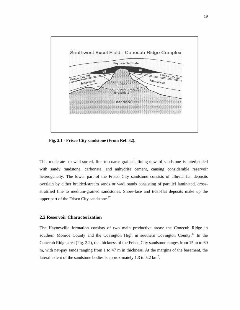
produced from 13 Frisco City fields.28 The Frisco City field contains a combined structural

stratigraphic trap. A basement anticline forms the structural part, while the stratigraphic

component is caused by pinching out of the porous sandstone against the basement paleo high

(Fig. 2.1).

2.1 Depositional Environment and Reservoir Facies

Since the discovery, several models have been proposed for the depositional environment of the

Late Jurassic Frisco City sand. Mann et al.29 interpreted the Frisco City sand to represent a

shallow marine, braid delta-front; Stephenson et al.30 suggested braided stream deposits

associated with alluvial fans, while Kugler and Mink31 interpreted this sand to represent strand

plain/beach deposits associated with braid deltas.32 Hill and Halvatzis33 even identified eight

depositional environments in their paper. Beside the depositional environments mentioned

earlier, they also suggest other environments that could include wadi deposits, aeolian deposits,

shoal-water braided-delta-front deposits, tidal channel and ebb, and braided-delta deposits, and

beach/shore face deposits. After conducting core analysis, Hill and Halvatzis suggest that the

Frisco City sand has a number of depositional environments, indicating that it may include all

eight depositional settings.

19

Fig. 2.1 - Frisco City sandstone (From Ref. 32).

This moderate- to well-sorted, fine to coarse-grained, fining-upward sandstone is interbedded

with sandy mudstone, carbonate, and anhydrite cement, causing considerable reservoir

heterogeneity. The lower part of the Frisco City sandstone consists of alluvial-fan deposits

overlain by either braided-stream sands or wadi sands consisting of parallel laminated, cross-

stratified fine to medium-grained sandstones. Shore-face and tidal-flat deposits make up the

upper part of the Frisco City sandstone.27

2.2 Reservoir Characterization

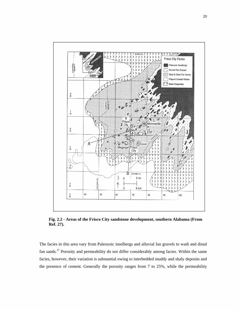
The Haynesville formation consists of two main productive areas: the Conecuh Ridge in

southern Monroe County and the Covington High in southern Covington County.33 In the

Conecuh Ridge area (Fig. 2.2), the thickness of the Frisco City sandstone ranges from 15 m to 60

m, with net-pay sands ranging from 1 to 47 m in thickness. At the margins of the basement, the

lateral extent of the sandstone bodies is approximately 1.3 to 5.2 km2.

20

Fig. 2.2 - Areas of the Frisco City sandstone development, southern Alabama (From Ref. 27).

The facies in this area vary from Paleozoic inselbergs and alluvial fan gravels to wadi and distal

fan sands.27 Porosity and permeability do not differ considerably among facies. Within the same

facies, however, their variation is substantial owing to interbedded muddy and shaly deposits and

the presence of cement. Generally the porosity ranges from 7 to 25%, while the permeability

21

ranges from 0.10 to 5,000 md. The average porosity is 21% and the average permeability is 250

md.29,32,33

2.3 Available Data

The Frisco City sand core samples used in this study are from the McCall 25-9 well, North

Frisco City (Paramount) field, Monroe County, Alabama. This well is located in the North Frisco

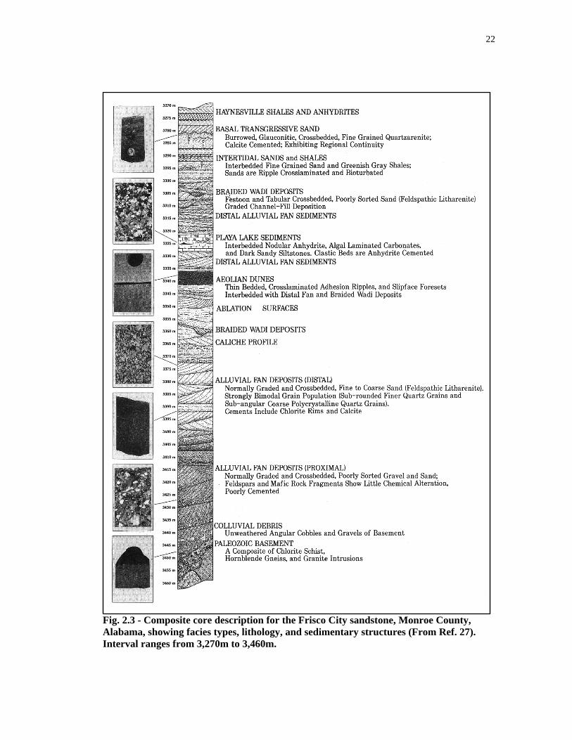
City sandstone (Fig. 2.2). Fig. 2.3 represents a core description of the Frisco City sandstone,

showing facies types, lithology, and sedimentary structures.

There are two sets of core with depths of 11,975 to 11,987 ft (Dataset 1) and 12,014 to 12,026 ft

(Dataset 2). The facies present in the cored intervals are stacked, braided, alluvial deposits. Core-

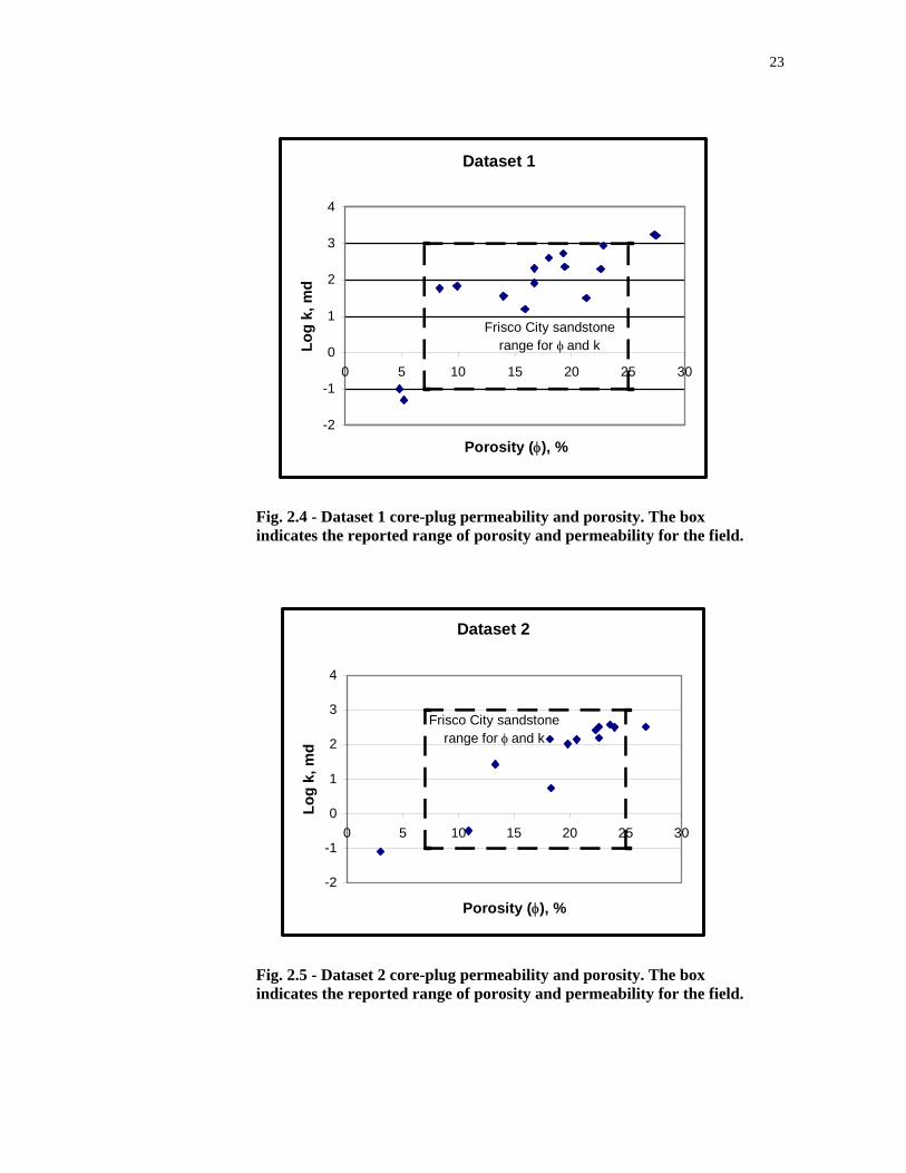
plug data (Figs. 2.4 and 2.5) indicate that the porosity and permeability are consistent with

values reported for the formation.

I described the two cored intervals geologically by visual inspection (Appendix B, Tables B-1

and B-2). Core-plug permeability data were available and I used a probe permeameter to

determine probe permeabilities of the two intervals. Furthermore, there are data available from

porosity, density, gamma ray, SP, caliper, resistivity and photo-electric logs. These data are

further described in Chap. III.

22

Fig. 2.3 - Composite core description for the Frisco City sandstone, Monroe County, Alabama, showing facies types, lithology, and sedimentary structures (From Ref. 27). Interval ranges from 3,270m to 3,460m.

23

Dataset 1

-2

-1

0

1

2

3

4

0 5 10 15 20 25 30

Porosity (φ), %

Log

k, m

dFrisco City sandstone

range for φ and k

Fig. 2.4 - Dataset 1 core-plug permeability and porosity. The box indicates the reported range of porosity and permeability for the field.

Dataset 2

-2

-1

0

1

2

3

4

0 5 10 15 20 25 30

Porosity (φ), %

Log

k, m

d

Frisco City sandstonerange for φ and k

Fig. 2.5 - Dataset 2 core-plug permeability and porosity. The box indicates the reported range of porosity and permeability for the field.

24

CHAPTER III

DATA COLLECTION

For this research, I analyzed and compared probe-, core-plug-, and log-derived permeabilities.

Therefore, I will give a brief overview of these methods of permeability determination.

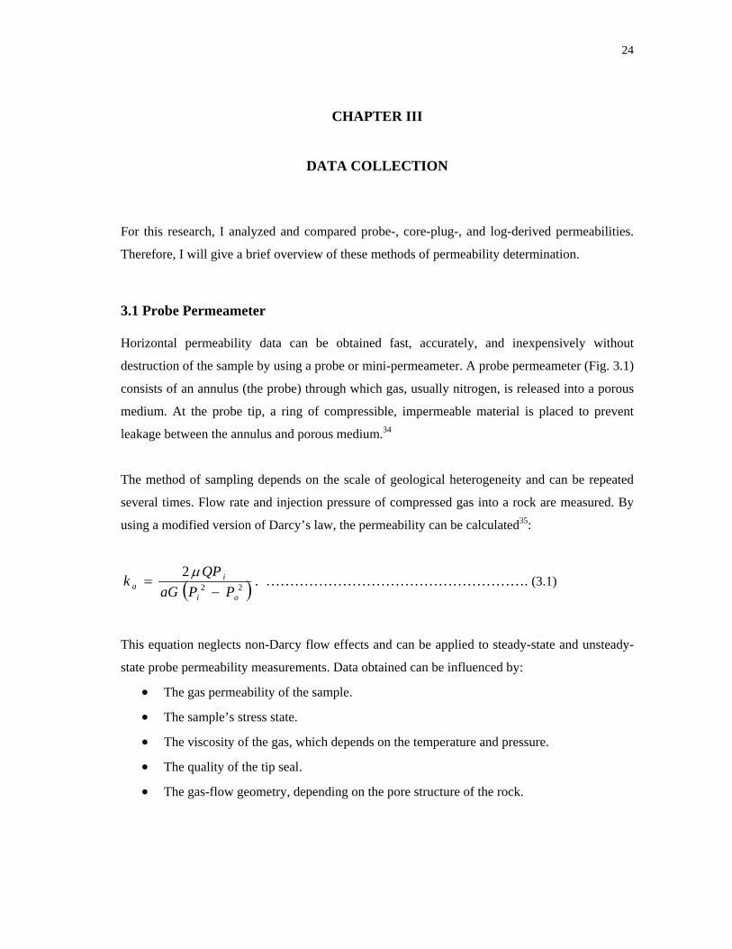
3.1 Probe Permeameter

Horizontal permeability data can be obtained fast, accurately, and inexpensively without

destruction of the sample by using a probe or mini-permeameter. A probe permeameter (Fig. 3.1)

consists of an annulus (the probe) through which gas, usually nitrogen, is released into a porous

medium. At the probe tip, a ring of compressible, impermeable material is placed to prevent

leakage between the annulus and porous medium.34

The method of sampling depends on the scale of geological heterogeneity and can be repeated

several times. Flow rate and injection pressure of compressed gas into a rock are measured. By

using a modified version of Darcy’s law, the permeability can be calculated35:

( )22

2

oi

ia PPaG

QPk−

=µ . ………………………………………………. (3.1)

This equation neglects non-Darcy flow effects and can be applied to steady-state and unsteady-

state probe permeability measurements. Data obtained can be influenced by:

• The gas permeability of the sample.

• The sample’s stress state.

• The viscosity of the gas, which depends on the temperature and pressure.

• The quality of the tip seal.

• The gas-flow geometry, depending on the pore structure of the rock.

25

Usually probe permeability measurements can be taken more frequently than core plugs, making

adjustment of core-plug to log depth more accurate.36 Especially for finely laminated rock

samples, the higher number of samples can detect the permeability variations caused by

heterogeneity, which would not have been detected with conventional core plugs.

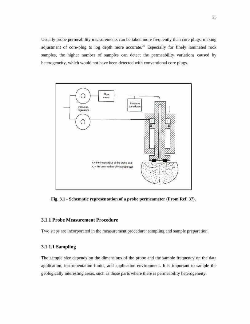
Fig. 3.1 - Schematic representation of a probe permeameter (From Ref. 37).

3.1.1 Probe Measurement Procedure

Two steps are incorporated in the measurement procedure: sampling and sample preparation.

3.1.1.1 Sampling

The sample size depends on the dimensions of the probe and the sample frequency on the data

application, instrumentation limits, and application environment. It is important to sample the

geologically interesting areas, such as those parts where there is permeability heterogeneity.

26

Hurst and Rosvoll38 suggested that the number of samples in clastic reservoirs can be calculated

with the following formula, commonly recognized as the “No rule of thumb” equation:

( 210 Vo CN = ) . ………………………….……………………. (3.2)

The coefficient of variation (CV) is the standard deviation divided by the mean. CV remains

relatively constant even if the data are from different sources, because both the mean and

standard deviation change. 25

3.1.1.2 Sample preparation

Ideally, samples should be dry and clean so we can completely saturate them with gas and apply

Darcy’s law. However, the sample preparation depends on the objectives of the experiment.39

For example, when the cores are not cleaned and dried, the effective permeability at unknown oil

and water saturation is measured.37

3.1.2 Probe Data Acquisition

• Preset sample spacing on an x-y grid.

• Check for visible areas, such as fractures or uneven surfaces, that might prevent

accurate sealing.

• Select an appropriate tip size [Two seals were available: a medium seal (23 mm

outer diameter) and a large seal (33 mm outer diameter).].

• Record the probe position on the rock sample.

• Control the force applied to the probe tip seal.

• Program the margin allowed for deviation from the constant gas-flow rate.

• Proceed to steady-state measurements and keep monitoring them.34

3.1.3 Problems and Limitations of Probe Permeametry

Even though probe permeametry has many advantages, it also has its limits. Some of the

limitations are:

27

• Uncleaned core samples obscure some pore spaces

Residual reservoir oil and salt contamination from the drilling mud present in the

core samples can influence probe measurements. The readings will be too low

since some of the pore space is occupied by the contamination.

• Measurements are taken on unstressed cores

Sandstones have lower permeabilities at in-situ conditions where they are subject

to confining pressures.40

• The effect of heterogeneity is not determined on macro scale

The heterogeneity is only determined at the wellbore.41

A detailed discussion of probe permeametry, advantages and limitations is presented in Ref. 37.

3.1.4 Probe Measurements on McCall 25-9 Core

I measured the probe permeabilities on Datasets 1 and 2 using the large seal. For the first dataset

I also used the medium seal to determine the effect of different seal sizes. Furthermore, I

determined the permeabilities at the same depths where core plugs had been taken and took some

additional measurements, too. The extra measurements were taken at geologically interesting

points, i.e. where there was a variation in lithology. I did not apply the No rule of thumb, since I

would need a large number of samples (see 4.3.1).

3.2 Core Plugs

Core plugs are usually taken to determine the lithology of the reservoir rock and establish

physical rock properties. With these data, we can divide the reservoir into zones and determine

the geometry, continuity, and characteristics of these zones.18

28

3.2.1 Measurement Procedure

3.2.1.1 Sampling

As mentioned in Sec. 1.3.3, horizontal plugs are taken about every foot from cores, while

vertical plugs are taken less frequently, perhaps once per 3 to 5 ft upon request. Core plugs are

approximately 4 cm long, but are cut to 2.5 cm to eliminate mud-invaded parts. Plug diameters

range from 2.5 to 3.8 cm. After cutting the plugs, the cores may be slabbed into three parts. The

first part is used for geological analysis, the second part is for curation, and the third part is

usually required by a licensing agency.

The main purpose of core analysis is to establish the porosity and permeability variation as a

function of position and depth in a well.40

Analysis of core plugs can include the determination of:

• Porosity.

• Horizontal air permeability.

• Vertical air permeability.

• Relative permeability.

• Grain density.

• Capillary pressure.

• Cementation and saturation exponents.42

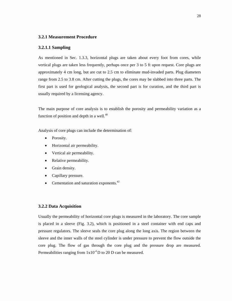
3.2.2 Data Acquisition

Usually the permeability of horizontal core plugs is measured in the laboratory. The core sample

is placed in a sleeve (Fig. 3.2), which is positioned in a steel container with end caps and

pressure regulators. The sleeve seals the core plug along the long axis. The region between the

sleeve and the inner walls of the steel cylinder is under pressure to prevent the flow outside the

core plug. The flow of gas through the core plug and the pressure drop are measured.

Permeabilities ranging from 1x10-4 D to 20 D can be measured.

29

Fig. 3.2 - A Hassler sleeve used to measure core-plug permeability (From Ref. 37).

3.2.3 Problems and Limitations of Core Plugs

The use of core plugs to determine permeabilities is subject to some limitations such as:

• The core plugs may not be representative of the surrounding reservoir rock.

The rock properties in the wellbore may be completely different from those

further away in the reservoir.41 Even at the wellbore, thin, impermeable layers

may not be detected because the core-plug spacing is relatively large.

• The effect of heterogeneity is only determined on a micro scale.

The effect of the macro-scale heterogeneity of the reservoir is not captured,

which in turn can affect the fluid flow.43 This problem applies to probe

measurements as well.

A detailed discussion of core-plug measurement procedures, advantages and limitations is

presented in Ref. 37.

30

3.2.4 Plug Data for McCall 25-9

The core-plug data available for the McCall 25-9 well, include measurements taken every foot

during routine core analysis for intervals of 11,956 to 11,996 ft and 12,014 to 12,041 ft. The core

plugs were not necessarily taken in the middle of the one-foot interval, but rather at geologically

interesting depths.

3.3 Core Plugs versus Probe Permeametry

Effective in-situ reservoir permeability can be estimated by using core-plug or probe

measurements. However, core plugs only measure the permeability approximately every foot (30

cm) and are therefore suitable for measuring permeability in relatively homogenous reservoirs.

Because of the relatively large sample spacing, thin, low-permeability layers may not be

detected. Core-plug measurements can be taken at reservoir stress to which the in-situ rock is

exposed.

The permeability can be measured more frequently with the probe permeameter, which measures

the absolute gas permeability of unstressed, uncleaned cores at a small volume scale. In

heterogeneous reservoirs I would recommend the use of the probe permeameter since local

heterogeneity in thin reservoir units can be determined more accurately than with core plugs

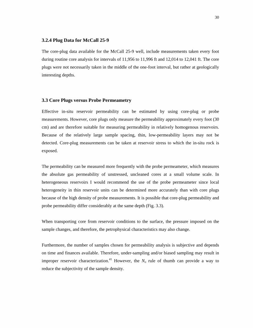
because of the high density of probe measurements. It is possible that core-plug permeability and

probe permeability differ considerably at the same depth (Fig. 3.3).

When transporting core from reservoir conditions to the surface, the pressure imposed on the

sample changes, and therefore, the petrophysical characteristics may also change.

Furthermore, the number of samples chosen for permeability analysis is subjective and depends

on time and finances available. Therefore, under-sampling and/or biased sampling may result in

improper reservoir characterization.41 However, the No rule of thumb can provide a way to

reduce the subjectivity of the sample density.

31

Core-plug permeability

Probe permeability (mD)

Fig. 3.3 - Difference in values between probe and core-plug permeability at the same depth (From Ref. 44). The core-plug value is very close to the arithmetic average of the permeability of the layers from which the plug comes.

3.4 Log Data

More accurate measures of reservoir zonation and volumetrics can be obtained by correlating log

data with either core-plug or probe data.45 For this research, I correlated core-plug data with the

wireline log data.

3.4.1 Measurement Procedure

There are several types of well logging such as measurement while drilling, mud logging, and

wireline logging. All these measurements are performed with the purpose of obtaining reservoir

properties.

32

3.4.2 Data Acquisition

There are a variety of well logging methods that can be applied, depending on the data we want

to acquire. Log measurements are taken every foot. However, the quality of the data can be

affected by borehole conditions and other factors.

3.4.3 Problems and Limitations of Well Logs

Several factors can influence the accuracy of well logs:

• Borehole Conditions

While drilling in permeable intervals, the drilling mud invades the formation and

forms a mudcake on the borehole wall. This happens when the pressure of the

mud column is larger than the formation pressure. A washout occurs when the

formation pressure is larger than the pressure of the mud column.

When excessive, these conditions can leads to equipment failure and abnormal

curve responses.

• Depth Shifts

Usually the logger’s depth and the driller’s depth are different. Therefore, it is

necessary to incorporate a depth shift when comparing log data to core data.46

Another limitation is the fact that logs may not be representative of the surrounding rock. Even

though they have a larger radius of investigation than core plugs, the macro heterogeneity of the

reservoir may not be captured.

3.4.4 Log Data for McCall 25-9

Several log measurements are available for the McCall 25-9 well. These include logs such as

density, neutron, gamma ray, spontaneous potential, photoelectric, and caliper. For this study I

used only the density and neutron logs. There seems to be a large depth shift present on these

logs.

33

3.5 Core-Plug versus Log Data

For a better petrophysical analysis, core-plug data and well log data have to be compared. For

the comparison with core-plug permeability, I used the density and neutron logs. Before

interpreting the logs, I did a quality check to determine the depth shift between the logger’s

depth and the driller’s depth.

Average reservoir properties are recorded at half- or whole-foot intervals on well logs at in-situ

conditions, whereas core-plug measurements only represent that part of the formation where the

core has been cut. Furthermore, core-plug measurements are taken at surface conditions and may

therefore not represent true reservoir properties.

Obviously, there is a difference in sample volume for log and core data. We can solve this

problem by using geostatistics:

• Log porosity should be computed as the volume-weighted arithmetic average

from core data.

• The average porosity value has a probable error, which is proportional to the

inverse square root of total volumes of cores analyzed.47

34

CHAPTER IV

DATA ANALYSIS

4.1 Investigation of the Frisco City Sandstone

I compared the probe permeameter permeability with the core-plug measurements and log

responses. These comparisons used various statistical averaging methods and correlations and

the geological description of the core.

These comparisons determine:

• How the different measurements are responding to geological variation.

• The effects of geology on net-pay evaluations.

• The effects of sampling and measurement type on net-pay and kv/kh estimates.

4.2 Lithological Assessment of the Core

As discussed in Chap. II, the two datasets are geologically similar. Both intervals consist of

sandstone interbedded with calcite cementing. Some thin shale layers are also present.

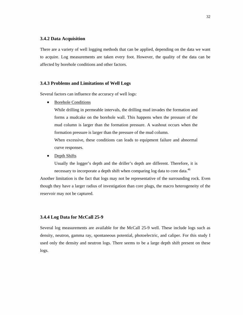
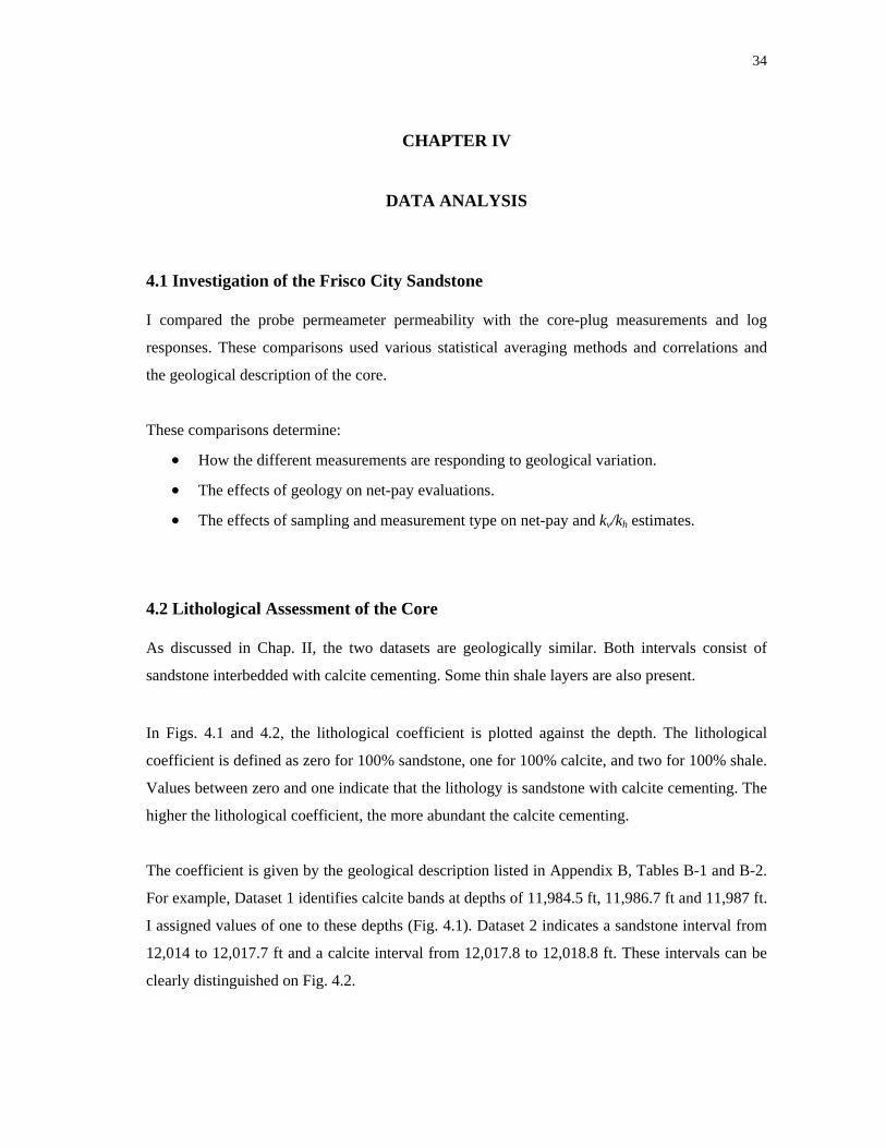
In Figs. 4.1 and 4.2, the lithological coefficient is plotted against the depth. The lithological

coefficient is defined as zero for 100% sandstone, one for 100% calcite, and two for 100% shale.

Values between zero and one indicate that the lithology is sandstone with calcite cementing. The

higher the lithological coefficient, the more abundant the calcite cementing.

The coefficient is given by the geological description listed in Appendix B, Tables B-1 and B-2.

For example, Dataset 1 identifies calcite bands at depths of 11,984.5 ft, 11,986.7 ft and 11,987 ft.

I assigned values of one to these depths (Fig. 4.1). Dataset 2 indicates a sandstone interval from

12,014 to 12,017.7 ft and a calcite interval from 12,017.8 to 12,018.8 ft. These intervals can be

clearly distinguished on Fig. 4.2.

35

Dataset 1

11974

11976

11978

11980

11982

11984

11986

0 0.5 1 1.5 2

Lithology coefficient

Dep

th (f

t)

sand

ston

e

shal

elimestone

Fig. 4.1 - Assessment of the lithological behavior of Dataset 1 with depth.

Dataset 2

12014

12016

12018

12020

12022

12024

12026

0 0.5 1 1.5 2

Lithology coefficient

Dep

th (f

t)

shal

e

sand

ston

e

limestone

Fig. 4.2 - Assessment of the lithological behavior of Dataset 2 with depth.

36

The determination of the lithological coefficient is somewhat arbitrary, since it is based on visual

inspection of the core. I did this twice to reduce the amount of human error. The results were

almost identical. The lithological coefficient was used in correlations described below.

4.3 Data Comparison

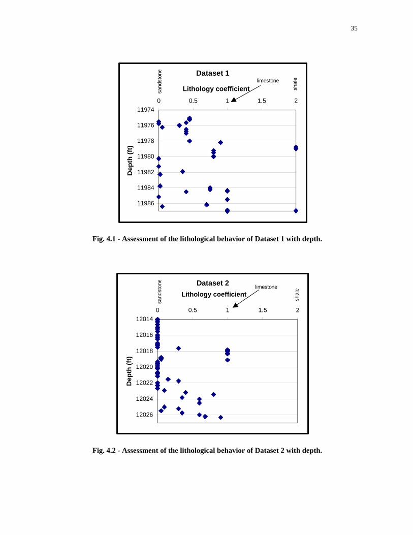
4.3.1 Analysis of the Effect of Different Probe Seal Sizes and the Lithology

As mentioned in Chap. III, I measured the probe permeability with a probe permeameter. For the

probe measurements of Dataset 1, I used a medium and a large tip. Fig. 4.3 shows the lithology

and probe permeabilities obtained with both tips.

Dataset 1

0.1

1

10

100

1000

10000

11974 11978 11982 11986

Depth (ft)

Prob

e pe

rmea

bilit

y ( k

), m

d

0

1

2

3

4

5

6

7

8

Lith

olog

y C

oeffi

cien

t

Medium Tip Large Tip Lithology Coefficient

Fig. 4.3 - Assessment of the effect of different tip sizes and their relation to the lithology.

The probe measurements seem to agree quite well, even though the large tip gives values that are

slightly pessimistic compared to the medium tip. This is because the large tip averages values

37

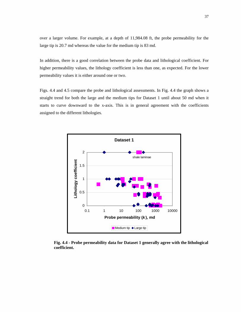
over a larger volume. For example, at a depth of 11,984.08 ft, the probe permeability for the

large tip is 20.7 md whereas the value for the medium tip is 83 md.

In addition, there is a good correlation between the probe data and lithological coefficient. For

higher permeability values, the lithology coefficient is less than one, as expected. For the lower

permeability values it is either around one or two.

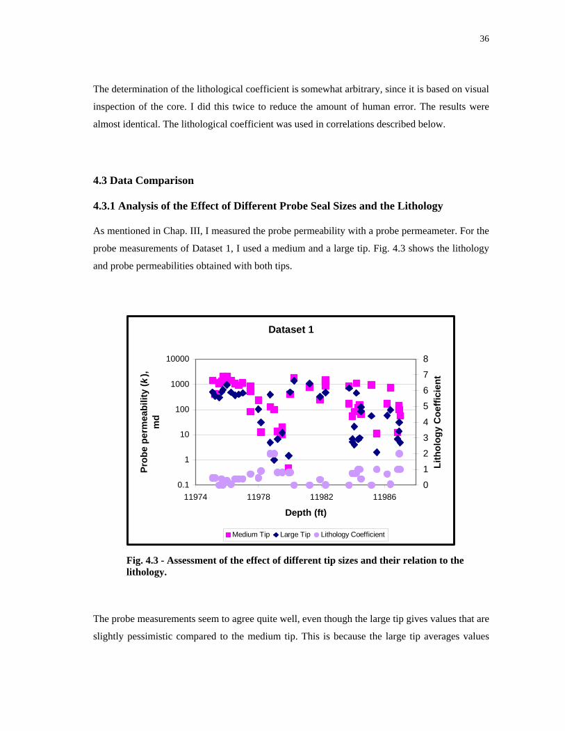
Figs. 4.4 and 4.5 compare the probe and lithological assessments. In Fig. 4.4 the graph shows a

straight trend for both the large and the medium tips for Dataset 1 until about 50 md when it

starts to curve downward to the x-axis. This is in general agreement with the coefficients

assigned to the different lithologies.

Dataset 1

0

0.5

1

1.5

2

0.1 1 10 100 1000 10000

Probe permeability (k ), md

Lith

olog

y co

effic

ient

Medium tip Large tip

shale laminae

Fig. 4.4 - Probe permeability data for Dataset 1 generally agree with the lithological coefficient.

38

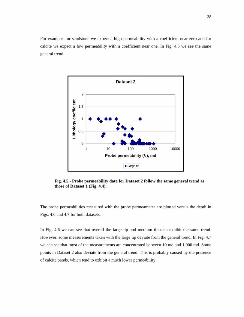
For example, for sandstone we expect a high permeability with a coefficient near zero and for

calcite we expect a low permeability with a coefficient near one. In Fig. 4.5 we see the same

general trend.

Dataset 2

0

0.5

1

1.5

2

1 10 100 1000 10000

Probe permeability (k ), md

Lith

olog

y co

effic

ient

Large tip

Fig. 4.5 - Probe permeability data for Dataset 2 follow the same general trend as those of Dataset 1 (Fig. 4.4).

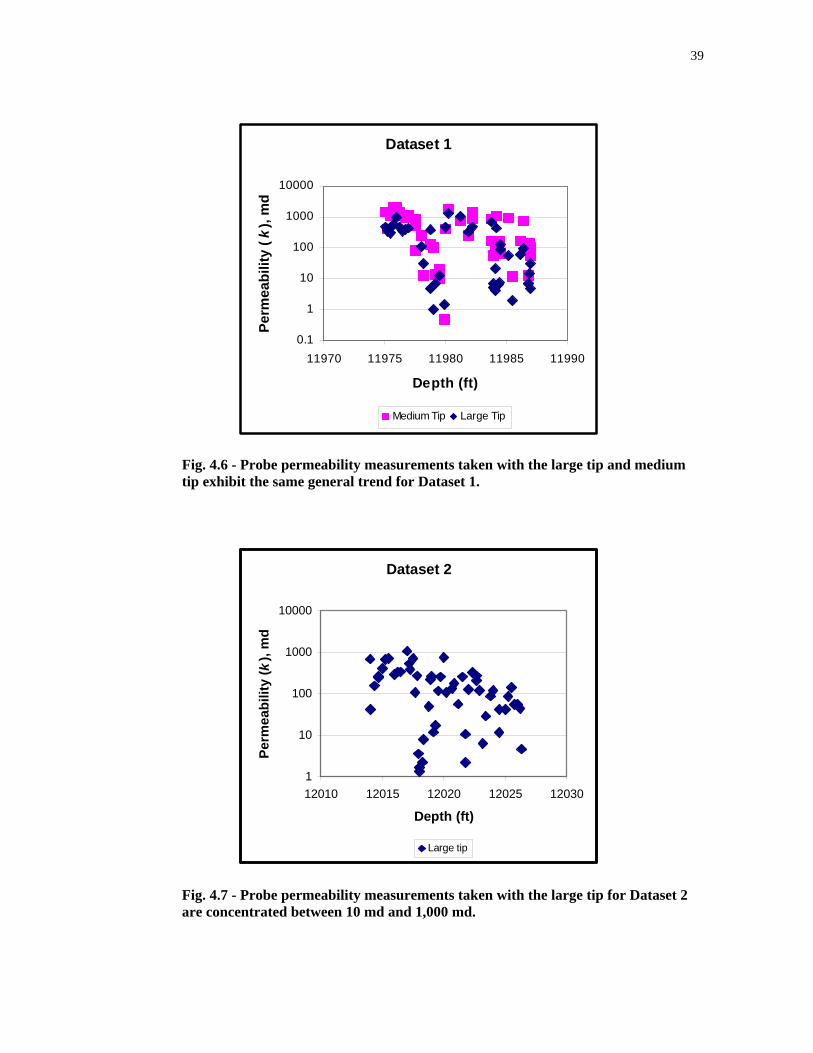
The probe permeabilities measured with the probe permeameter are plotted versus the depth in

Figs. 4.6 and 4.7 for both datasets.

In Fig. 4.6 we can see that overall the large tip and medium tip data exhibit the same trend.

However, some measurements taken with the large tip deviate from the general trend. In Fig. 4.7

we can see that most of the measurements are concentrated between 10 md and 1,000 md. Some

points in Dataset 2 also deviate from the general trend. This is probably caused by the presence

of calcite bands, which tend to exhibit a much lower permeability.

39

Dataset 1

0.1

1

10

100

1000

10000

11970 11975 11980 11985 11990

Depth (ft)

Perm

eabi

lity

(k),

md

Medium Tip Large Tip

Fig. 4.6 - Probe permeability measurements taken with the large tip and medium tip exhibit the same general trend for Dataset 1.

Dataset 2

1

10

100

1000

10000

12010 12015 12020 12025 12030

Depth (ft)

Perm

eabi

lity

( k),

md

Large tip

Fig. 4.7 - Probe permeability measurements taken with the large tip for Dataset 2 are concentrated between 10 md and 1,000 md.

40

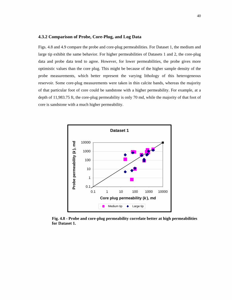
4.3.2 Comparison of Probe, Core-Plug, and Log Data

Figs. 4.8 and 4.9 compare the probe and core-plug permeabilities. For Dataset 1, the medium and

large tip exhibit the same behavior. For higher permeabilities of Datasets 1 and 2, the core-plug

data and probe data tend to agree. However, for lower permeabilities, the probe gives more

optimistic values than the core plug. This might be because of the higher sample density of the

probe measurements, which better represent the varying lithology of this heterogeneous

reservoir. Some core-plug measurements were taken in thin calcite bands, whereas the majority

of that particular foot of core could be sandstone with a higher permeability. For example, at a

depth of 11,983.75 ft, the core-plug permeability is only 70 md, while the majority of that foot of

core is sandstone with a much higher permeability.

Dataset 1

0.1

1

10

100

1000

10000

0.1 1 10 100 1000 10000

Core plug permeability (k ), md

Prob

e pe

rmea

bilit

y ( k

), m

d

Medium tip Large tip

Fig. 4.8 - Probe and core-plug permeability correlate better at high permeabilities for Dataset 1.

41

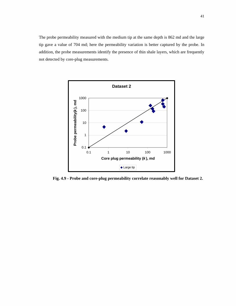
The probe permeability measured with the medium tip at the same depth is 862 md and the large

tip gave a value of 704 md; here the permeability variation is better captured by the probe. In

addition, the probe measurements identify the presence of thin shale layers, which are frequently

not detected by core-plug measurements.

Dataset 2

0.1

1

10

100

1000

0.1 1 10 100 1000

Core plug permeability (k ), md

Prob

e pe

rmea

bilit

y(k

), m

d

Large tip

Fig. 4.9 - Probe and core-plug permeability correlate reasonably well for Dataset 2.

42

I only used the large tip for Dataset 2 because the values obtained with the large tip for Dataset 1

seemed to match the core-plug values better than those obtained with the medium tip. However,

after analyzing the data, it seemed that the large tip values were slightly pessimistic since it

averages out over a larger volume. Therefore, for future probe analyses it is advisable to use the

medium tip.

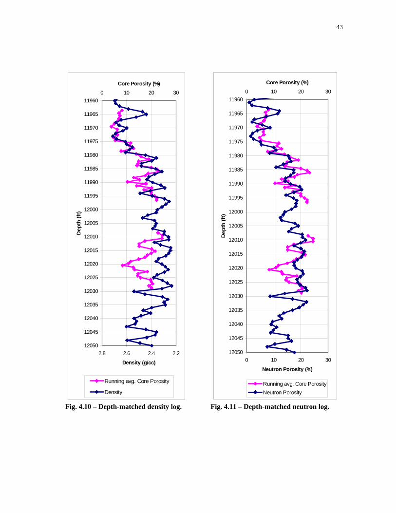
The log and core data were off depth. There is often a depth shift present because the logger’s

depth and the driller’s depth are different. To match the depth of these data, I used a three point

running average of the core-plug data. The core data are averaged since they are not taken at a

specific part within the foot they represent. The log data, on the other hand, are taken at a

specific part of the foot they represent and have a vertical resolution of about half a foot.

I shifted the core data 6 ft down for the first dataset and 6 ft up for the second dataset for both the

density and the neutron logs. Figs. 4.10 and 4.11, present the density and neutron logs after depth

matching.

It took several attempts to match the core-plug data with the log data. If the upper part matched

well, the lower part did not. I did not achieve a perfect match, but the log data agreed reasonably

well with the core-plug data after the final depth matching. Pay zones are easier to identify from

the log and core data together.

43

11960

11965

11970

11975

11980

11985

11990

11995

12000

12005

12010

12015

12020

12025

12030

12035

12040

12045

12050

0 10 20 30

Core Porosity (%)

Dep

th (f

t)

0 10 20 30

Neutron Porosity (%)

Running avg. Core PorosityNeutron Porosity

11960

11965

11970

11975

11980

11985

11990

11995

12000

12005

12010

12015

12020

12025

12030

12035

12040

12045

12050

0 10 20 30

Core Porosity (%)D

epth

(ft)

2.22.42.62.8

Density (g/cc)

Running avg. Core Porosity

Density

Fig. 4.10 – Depth-matched density log. Fig. 4.11 – Depth-matched neutron log.

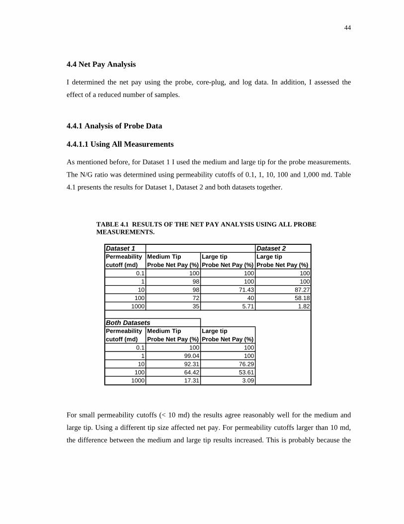
44

4.4 Net Pay Analysis

I determined the net pay using the probe, core-plug, and log data. In addition, I assessed the

effect of a reduced number of samples.

4.4.1 Analysis of Probe Data

4.4.1.1 Using All Measurements

As mentioned before, for Dataset 1 I used the medium and large tip for the probe measurements.

The N/G ratio was determined using permeability cutoffs of 0.1, 1, 10, 100 and 1,000 md. Table

4.1 presents the results for Dataset 1, Dataset 2 and both datasets together.

TABLE 4.1 RESULTS OF THE NET PAY ANALYSIS USING ALL PROBE MEASUREMENTS.

Dataset 1 Dataset 2Permeability Medium Tip Large tip Large tipcutoff (md) Probe Net Pay (%) Probe Net Pay (%) Probe Net Pay (%)

0.1 100 100 1001 98 100 100

10 98 71.43 87.27100 72 40 58.18

1000 35 5.71 1.82

Both DatasetsPermeability Medium Tip Large tipcutoff (md) Probe Net Pay (%) Probe Net Pay (%)

0.1 100 1001 99.04 100

10 92.31 76.29100 64.42 53.61

1000 17.31 3.09

For small permeability cutoffs (< 10 md) the results agree reasonably well for the medium and

large tip. Using a different tip size affected net pay. For permeability cutoffs larger than 10 md,

the difference between the medium and large tip results increased. This is probably because the

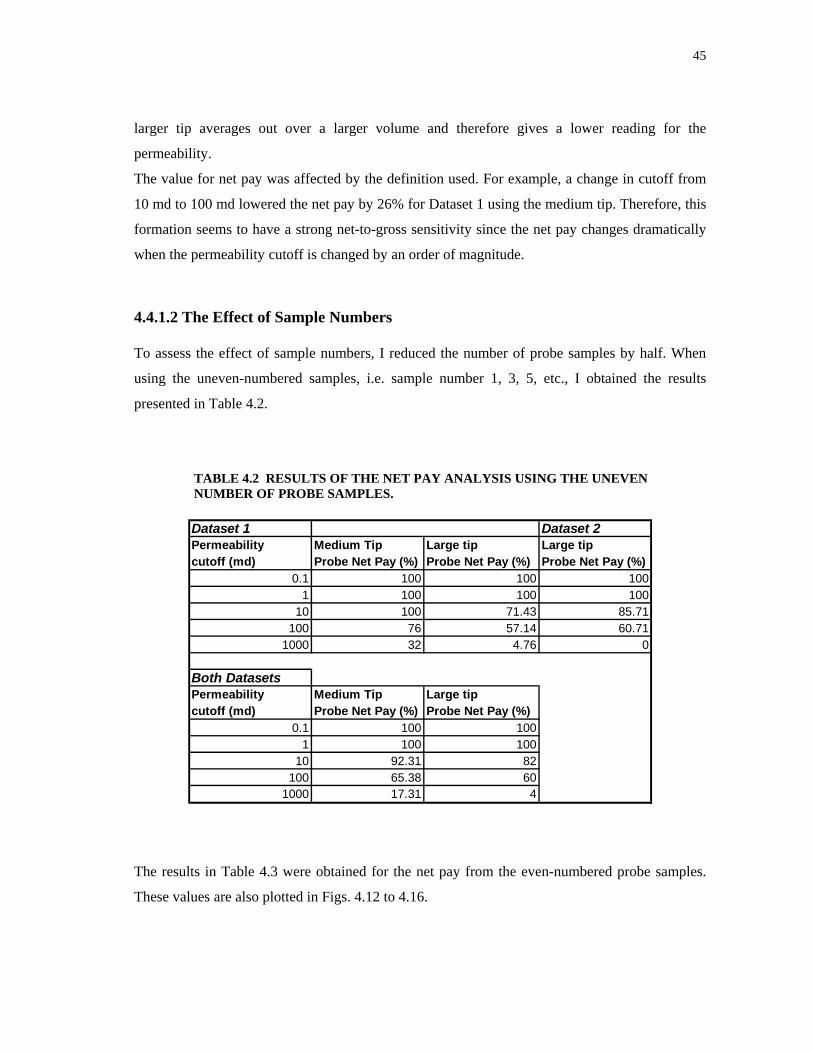
45

larger tip averages out over a larger volume and therefore gives a lower reading for the

permeability.

The value for net pay was affected by the definition used. For example, a change in cutoff from

10 md to 100 md lowered the net pay by 26% for Dataset 1 using the medium tip. Therefore, this

formation seems to have a strong net-to-gross sensitivity since the net pay changes dramatically

when the permeability cutoff is changed by an order of magnitude.

4.4.1.2 The Effect of Sample Numbers

To assess the effect of sample numbers, I reduced the number of probe samples by half. When

using the uneven-numbered samples, i.e. sample number 1, 3, 5, etc., I obtained the results

presented in Table 4.2.

TABLE 4.2 RESULTS OF THE NET PAY ANALYSIS USING THE UNEVEN NUMBER OF PROBE SAMPLES.

Dataset 1 Dataset 2Permeability Medium Tip Large tip Large tipcutoff (md) Probe Net Pay (%) Probe Net Pay (%) Probe Net Pay (%)

0.1 100 100 1001 100 100 100

10 100 71.43 85.71100 76 57.14 60.71

1000 32 4.76 0

Both DatasetsPermeability Medium Tip Large tipcutoff (md) Probe Net Pay (%) Probe Net Pay (%)

0.1 100 1001 100 100

10 92.31 82100 65.38 60

1000 17.31 4 The results in Table 4.3 were obtained for the net pay from the even-numbered probe samples.

These values are also plotted in Figs. 4.12 to 4.16.

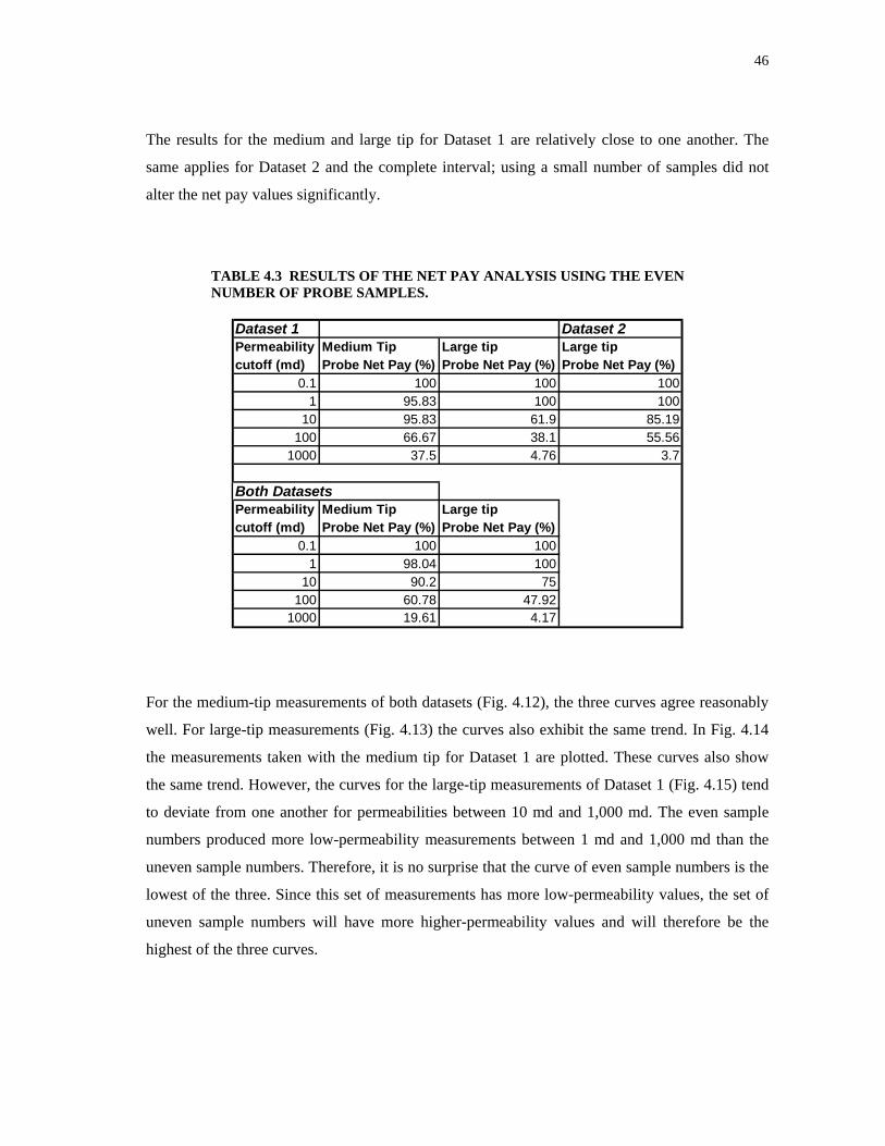
46

The results for the medium and large tip for Dataset 1 are relatively close to one another. The

same applies for Dataset 2 and the complete interval; using a small number of samples did not

alter the net pay values significantly.

TABLE 4.3 RESULTS OF THE NET PAY ANALYSIS USING THE EVEN NUMBER OF PROBE SAMPLES.

Dataset 1 Dataset 2Permeability Medium Tip Large tip Large tipcutoff (md) Probe Net Pay (%) Probe Net Pay (%) Probe Net Pay (%)

0.1 100 100 1001 95.83 100 100

10 95.83 61.9 85.19100 66.67 38.1 55.56

1000 37.5 4.76 3.7

Both DatasetsPermeability Medium Tip Large tipcutoff (md) Probe Net Pay (%) Probe Net Pay (%)

0.1 100 1001 98.04 100

10 90.2 75100 60.78 47.92

1000 19.61 4.17 For the medium-tip measurements of both datasets (Fig. 4.12), the three curves agree reasonably

well. For large-tip measurements (Fig. 4.13) the curves also exhibit the same trend. In Fig. 4.14

the measurements taken with the medium tip for Dataset 1 are plotted. These curves also show

the same trend. However, the curves for the large-tip measurements of Dataset 1 (Fig. 4.15) tend

to deviate from one another for permeabilities between 10 md and 1,000 md. The even sample

numbers produced more low-permeability measurements between 1 md and 1,000 md than the

uneven sample numbers. Therefore, it is no surprise that the curve of even sample numbers is the

lowest of the three. Since this set of measurements has more low-permeability values, the set of

uneven sample numbers will have more higher-permeability values and will therefore be the

highest of the three curves.

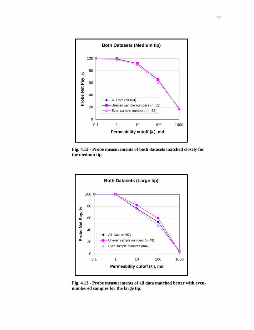
47

Both Datasets (Medium tip)

0

20

40

60

80

100

0.1 1 10 100 1000

Permeability cutoff (k ), md

Prob

e N

et P

ay, %

All Data (n=104)Uneven sample numbers (n=52)Even sample numbers (n=52)

Fig. 4.12 - Probe measurements of both datasets matched closely for the medium tip.

Both Datasets (Large tip)

0

20

40

60

80

100

0.1 1 10 100 1000

Permeability cutoff (k ), md

Prob

e N

et P

ay, %

All Data (n=97)

Uneven sample numbers (n=49)

Even sample numbers (n=48)

Fig. 4.13 - Probe measurements of all data matched better with even-numbered samples for the large tip.

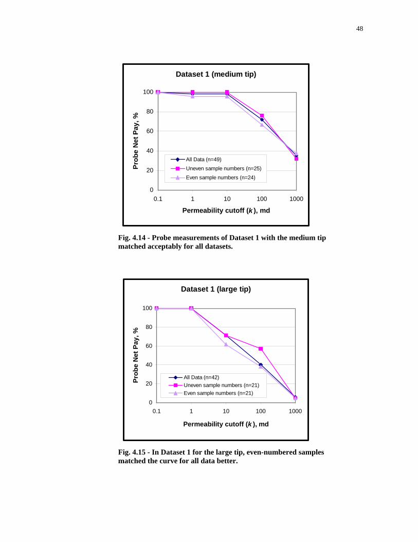
48

Dataset 1 (medium tip)

0

20

40

60

80

100

0.1 1 10 100 1000

Permeability cutoff (k ), md

Prob

e N

et P

ay, %

All Data (n=49)

Uneven sample numbers (n=25)

Even sample numbers (n=24)

Fig. 4.14 - Probe measurements of Dataset 1 with the medium tip matched acceptably for all datasets.

Dataset 1 (large tip)

0

20

40

60

80

100

0.1 1 10 100 1000

Permeability cutoff (k ), md

Prob

e N

et P

ay, %

All Data (n=42)Uneven sample numbers (n=21)Even sample numbers (n=21)

Fig. 4.15 - In Dataset 1 for the large tip, even-numbered samples matched the curve for all data better.

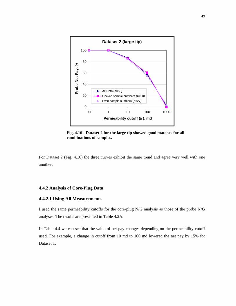
49

Dataset 2 (large tip)

0

20

40

60

80

100

0.1 1 10 100 1000

Permeability cutoff (k ), md

Prob

e N

et P

ay, %

All Data (n=55)Uneven sample numbers (n=28)Even sample numbers (n=27)

Fig. 4.16 - Dataset 2 for the large tip showed good matches for all combinations of samples.

For Dataset 2 (Fig. 4.16) the three curves exhibit the same trend and agree very well with one

another.

4.4.2 Analysis of Core-Plug Data

4.4.2.1 Using All Measurements

I used the same permeability cutoffs for the core-plug N/G analysis as those of the probe N/G

analyses. The results are presented in Table 4.2A.

In Table 4.4 we can see that the value of net pay changes depending on the permeability cutoff

used. For example, a change in cutoff from 10 md to 100 md lowered the net pay by 15% for

Dataset 1.

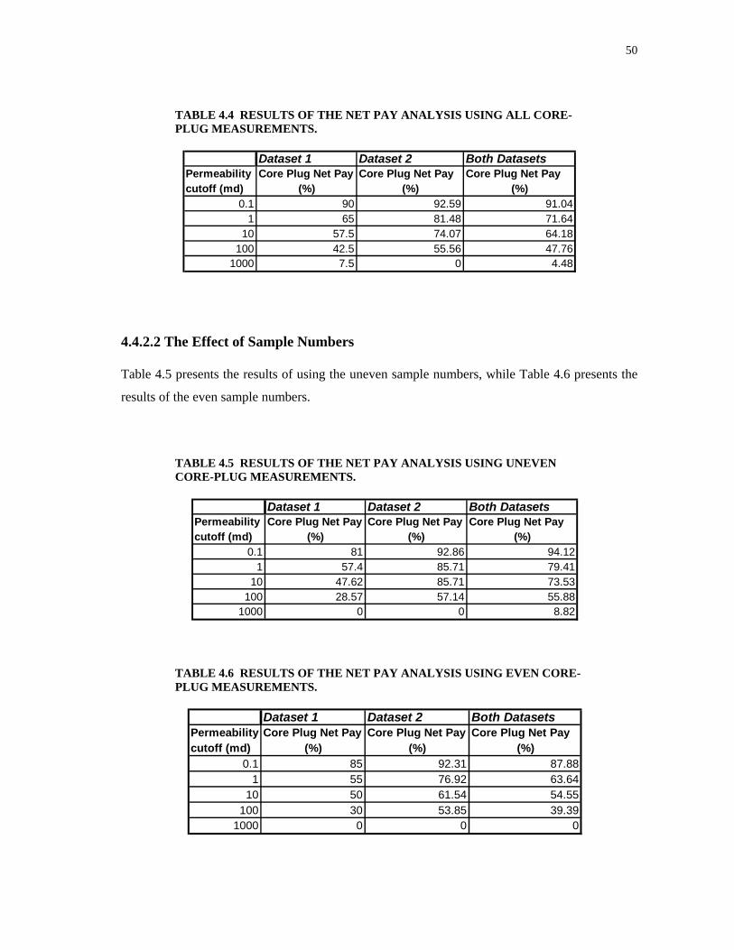
50

TABLE 4.4 RESULTS OF THE NET PAY ANALYSIS USING ALL CORE-PLUG MEASUREMENTS.

Dataset 1 Dataset 2 Both Datasets

Permeability Core Plug Net Pay Core Plug Net Pay Core Plug Net Pay cutoff (md) (%) (%) (%)

0.1 90 92.59 91.041 65 81.48 71.64

10 57.5 74.07 64.18100 42.5 55.56 47.76

1000 7.5 0 4.48

4.4.2.2 The Effect of Sample Numbers

Table 4.5 presents the results of using the uneven sample numbers, while Table 4.6 presents the

results of the even sample numbers.

TABLE 4.5 RESULTS OF THE NET PAY ANALYSIS USING UNEVEN CORE-PLUG MEASUREMENTS.

Dataset 1 Dataset 2 Both Datasets

Permeability Core Plug Net Pay Core Plug Net Pay Core Plug Net Pay cutoff (md) (%) (%) (%)

0.1 81 92.86 94.121 57.4 85.71 79.41

10 47.62 85.71 73.53100 28.57 57.14 55.88

1000 0 0 8.82

TABLE 4.6 RESULTS OF THE NET PAY ANALYSIS USING EVEN CORE-PLUG MEASUREMENTS.

Dataset 1 Dataset 2 Both Datasets

Permeability Core Plug Net Pay Core Plug Net Pay Core Plug Net Pay cutoff (md) (%) (%) (%)

0.1 85 92.31 87.881 55 76.92 63.64

10 50 61.54 54.55100 30 53.85 39.39

1000 0 0 0

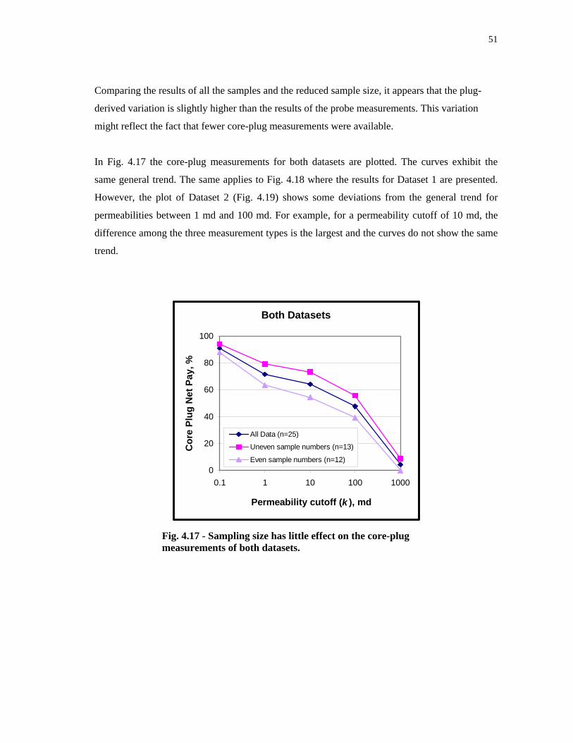
51

Comparing the results of all the samples and the reduced sample size, it appears that the plug-

derived variation is slightly higher than the results of the probe measurements. This variation

might reflect the fact that fewer core-plug measurements were available.

In Fig. 4.17 the core-plug measurements for both datasets are plotted. The curves exhibit the

same general trend. The same applies to Fig. 4.18 where the results for Dataset 1 are presented.

However, the plot of Dataset 2 (Fig. 4.19) shows some deviations from the general trend for

permeabilities between 1 md and 100 md. For example, for a permeability cutoff of 10 md, the

difference among the three measurement types is the largest and the curves do not show the same

trend.

Both Datasets

0

20

40

60

80

100

0.1 1 10 100 1000

Permeability cutoff (k ), md

Cor

e Pl

ug N

et P

ay, %

All Data (n=25)

Uneven sample numbers (n=13)

Even sample numbers (n=12)

Fig. 4.17 - Sampling size has little effect on the core-plug measurements of both datasets.

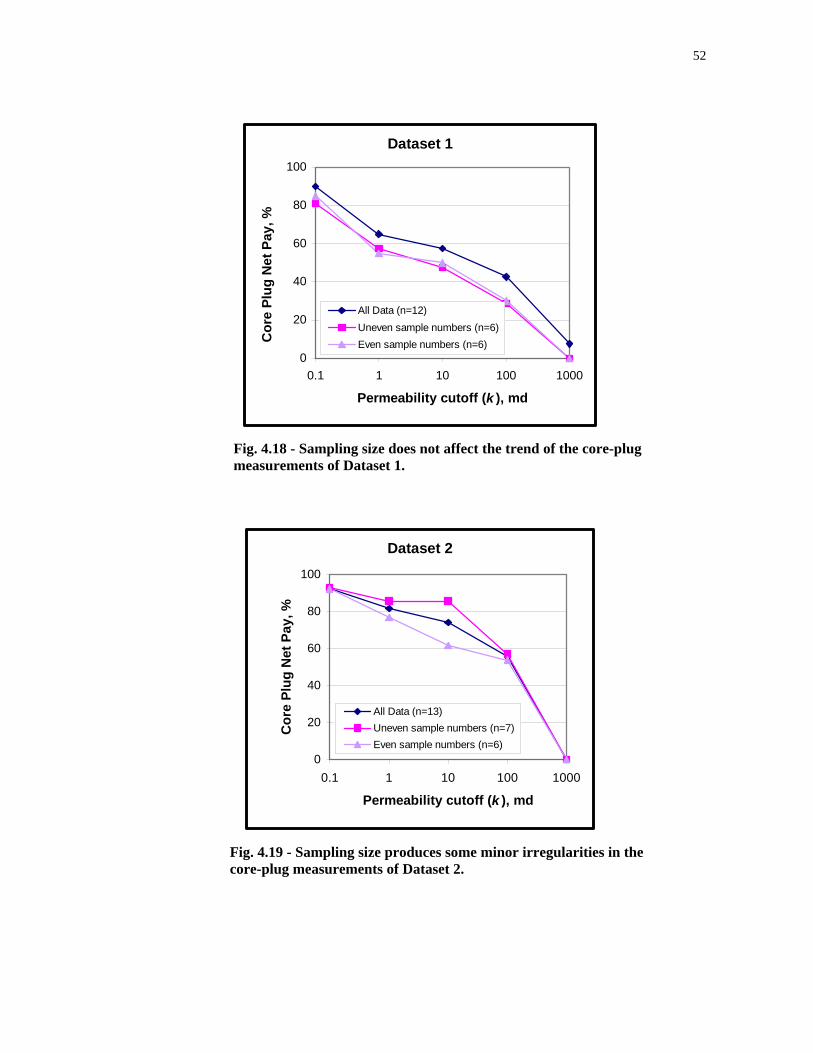
52

Dataset 1

0

20

40

60

80

100

0.1 1 10 100 1000

Permeability cutoff (k ), md

Cor

e Pl

ug N

et P

ay, %

All Data (n=12)Uneven sample numbers (n=6)Even sample numbers (n=6)

Fig. 4.18 - Sampling size does not affect the trend of the core-plug measurements of Dataset 1.

Dataset 2

0

20

40

60

80

100

0.1 1 10 100 1000

Permeability cutoff (k ), md

Cor

e Pl

ug N

et P

ay, %

All Data (n=13)Uneven sample numbers (n=7)Even sample numbers (n=6)

Fig. 4.19 - Sampling size produces some minor irregularities in the core-plug measurements of Dataset 2.

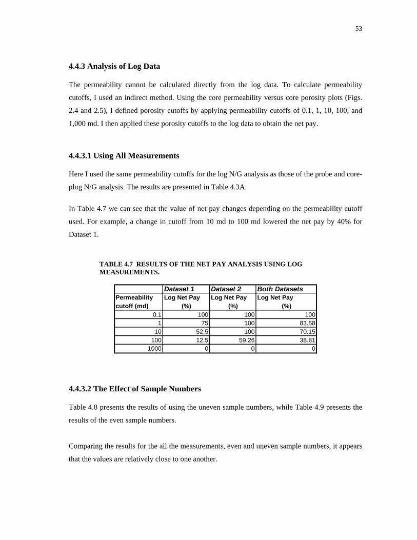
53

4.4.3 Analysis of Log Data

The permeability cannot be calculated directly from the log data. To calculate permeability

cutoffs, I used an indirect method. Using the core permeability versus core porosity plots (Figs.

2.4 and 2.5), I defined porosity cutoffs by applying permeability cutoffs of 0.1, 1, 10, 100, and

1,000 md. I then applied these porosity cutoffs to the log data to obtain the net pay.

4.4.3.1 Using All Measurements

Here I used the same permeability cutoffs for the log N/G analysis as those of the probe and core-

plug N/G analysis. The results are presented in Table 4.3A.

In Table 4.7 we can see that the value of net pay changes depending on the permeability cutoff

used. For example, a change in cutoff from 10 md to 100 md lowered the net pay by 40% for

Dataset 1.

TABLE 4.7 RESULTS OF THE NET PAY ANALYSIS USING LOG MEASUREMENTS.

Dataset 1 Dataset 2 Both Datasets

Permeability Log Net Pay Log Net Pay Log Net Paycutoff (md) (%) (%) (%)

0.1 100 100 1001 75 100 83.58

10 52.5 100 70.15100 12.5 59.26 38.81

1000 0 0 0 4.4.3.2 The Effect of Sample Numbers

Table 4.8 presents the results of using the uneven sample numbers, while Table 4.9 presents the

results of the even sample numbers.

Comparing the results for the all the measurements, even and uneven sample numbers, it appears

that the values are relatively close to one another.

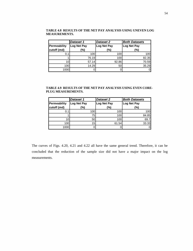
54

TABLE 4.8 RESULTS OF THE NET PAY ANALYSIS USING UNEVEN LOG MEASUREMENTS.

Dataset 1 Dataset 2 Both Datasets

Permeability Log Net Pay Log Net Pay Log Net Pay cutoff (md) (%) (%) (%)

0.1 100 100 1001 76.19 100 82.35

10 57.14 92.86 70.59100 14.29 50 35.29

1000 0 0 0

TABLE 4.9 RESULTS OF THE NET PAY ANALYSIS USING EVEN CORE-PLUG MEASUREMENTS.

Dataset 1 Dataset 2 Both Datasets

Permeability Log Net Pay Log Net Pay Log Net Pay cutoff (md) (%) (%) (%)

0.1 100 100 1001 75 100 84.85

10 50 100 69.7100 15 61.54 33.33

1000 0 0 0

The curves of Figs. 4.20, 4.21 and 4.22 all have the same general trend. Therefore, it can be

concluded that the reduction of the sample size did not have a major impact on the log

measurements.

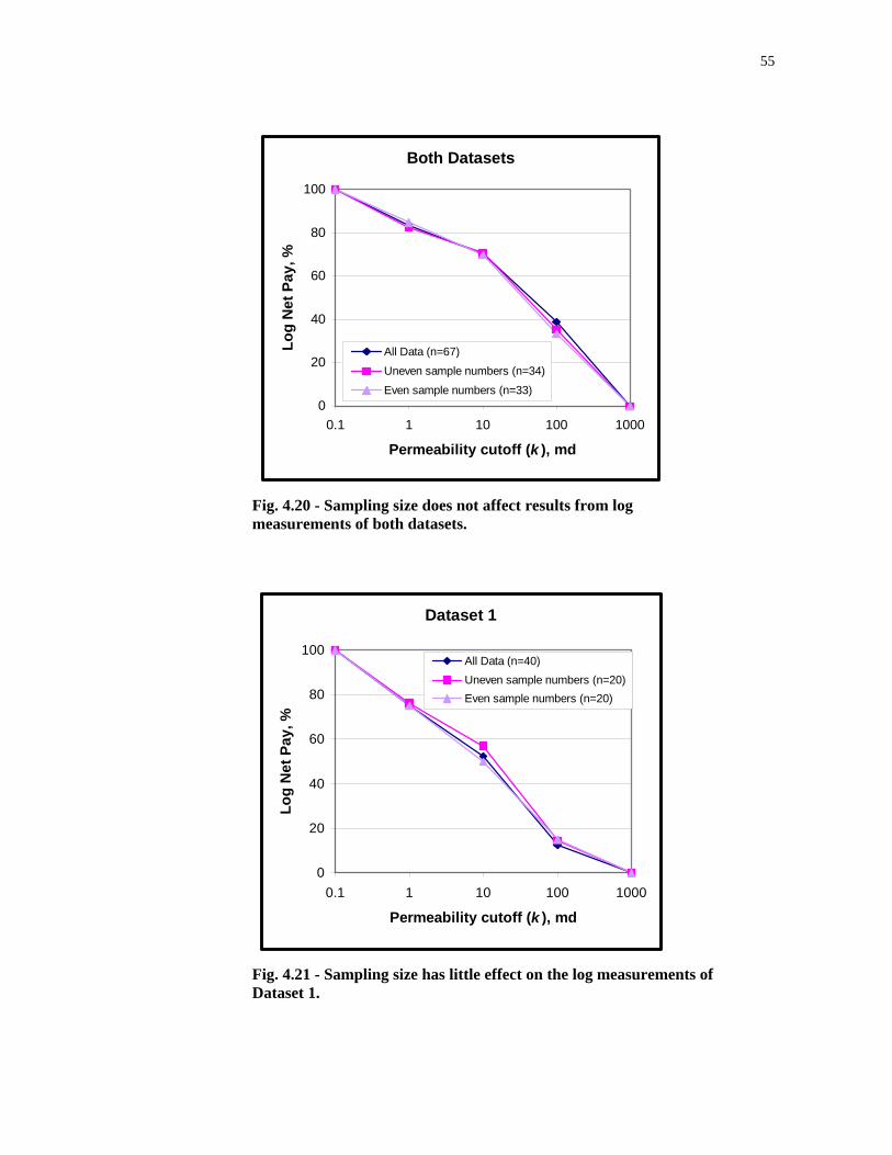
55

Both Datasets

0

20

40

60

80

100

0.1 1 10 100 1000

Permeability cutoff (k ), md

Log

Net

Pay

, %

All Data (n=67)

Uneven sample numbers (n=34)

Even sample numbers (n=33)

Fig. 4.20 - Sampling size does not affect results from log measurements of both datasets.

Dataset 1

0

20

40

60

80

100

0.1 1 10 100 1000

Permeability cutoff (k ), md

Log

Net

Pay

, %

All Data (n=40)Uneven sample numbers (n=20)Even sample numbers (n=20)

Fig. 4.21 - Sampling size has little effect on the log measurements of Dataset 1.

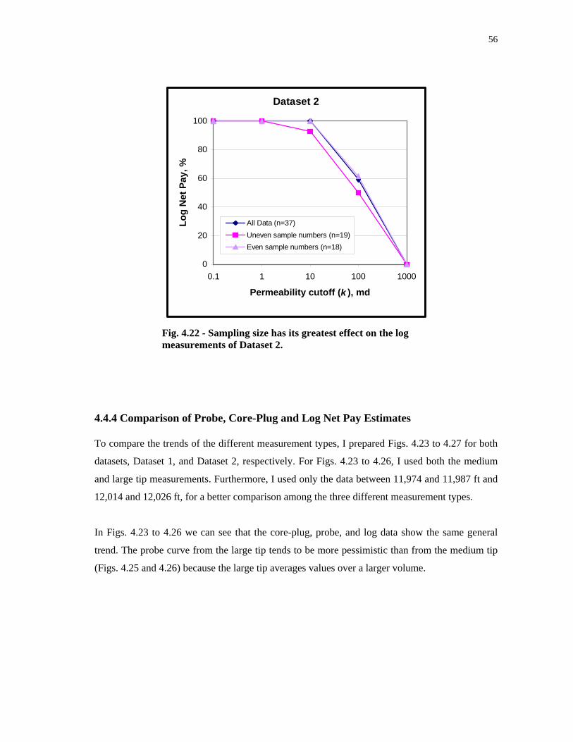
56

Dataset 2

0

20

40

60

80

100

0.1 1 10 100 1000

Permeability cutoff (k ), md

Log

Net

Pay

, %

All Data (n=37)Uneven sample numbers (n=19)Even sample numbers (n=18)

Fig. 4.22 - Sampling size has its greatest effect on the log measurements of Dataset 2.

4.4.4 Comparison of Probe, Core-Plug and Log Net Pay Estimates

To compare the trends of the different measurement types, I prepared Figs. 4.23 to 4.27 for both

datasets, Dataset 1, and Dataset 2, respectively. For Figs. 4.23 to 4.26, I used both the medium

and large tip measurements. Furthermore, I used only the data between 11,974 and 11,987 ft and

12,014 and 12,026 ft, for a better comparison among the three different measurement types.

In Figs. 4.23 to 4.26 we can see that the core-plug, probe, and log data show the same general

trend. The probe curve from the large tip tends to be more pessimistic than from the medium tip

(Figs. 4.25 and 4.26) because the large tip averages values over a larger volume.

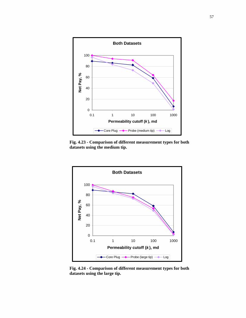
57

Both Datasets

0

20

40

60

80

100

0.1 1 10 100 1000

Permeability cutoff (k ), md

Net

Pay

, %

Core Plug Probe (medium tip) Log

Fig. 4.23 - Comparison of different measurement types for both datasets using the medium tip.

Both Datasets

0

20

40

60

80

100

0.1 1 10 100 1000

Permeability cutoff (k ), md

Net

Pay

, %

Core Plug Probe (large tip) Log

Fig. 4.24 - Comparison of different measurement types for both datasets using the large tip.

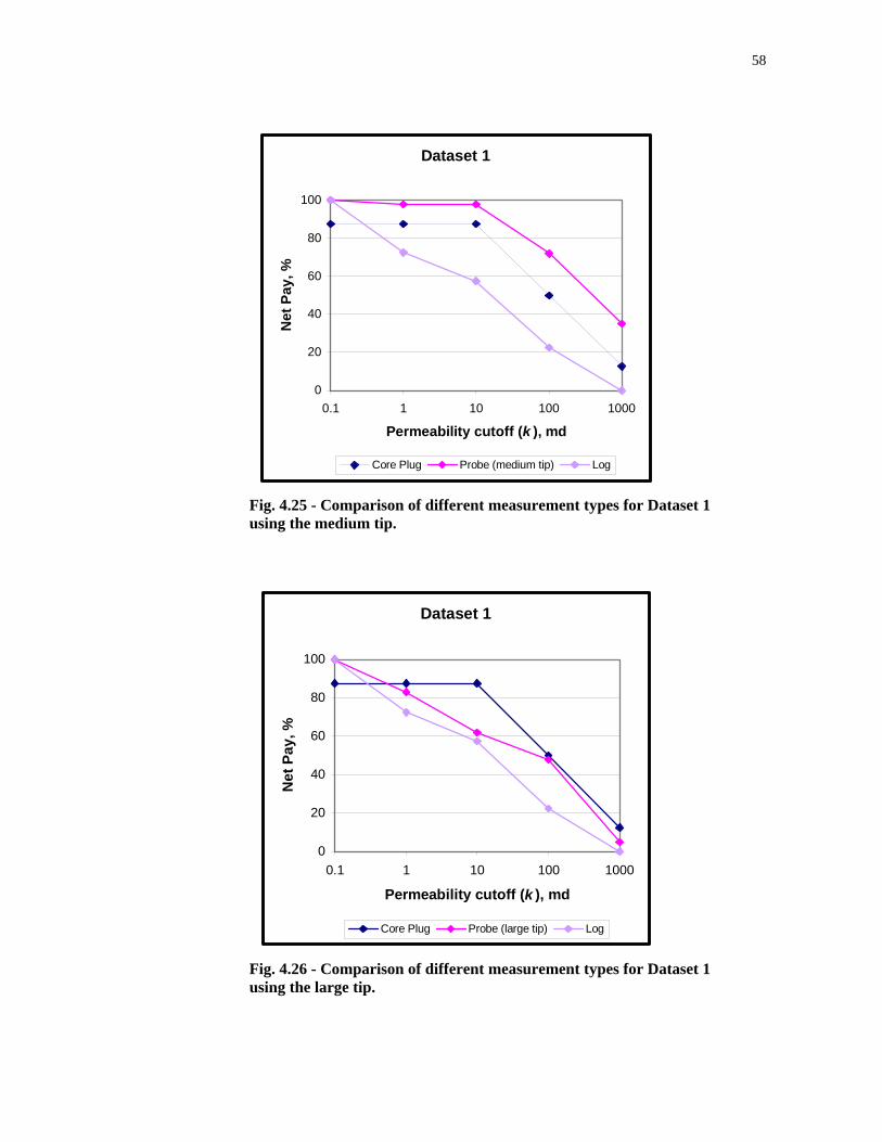
58

Dataset 1

0

20

40

60

80

100

0.1 1 10 100 1000

Permeability cutoff (k ), md

Net

Pay

, %

Core Plug Probe (medium tip) Log

Fig. 4.25 - Comparison of different measurement types for Dataset 1 using the medium tip.

Dataset 1

0

20

40

60

80

100

0.1 1 10 100 1000

Permeability cutoff (k ), md

Net

Pay

, %

Core Plug Probe (large tip) Log

Fig. 4.26 - Comparison of different measurement types for Dataset 1 using the large tip.

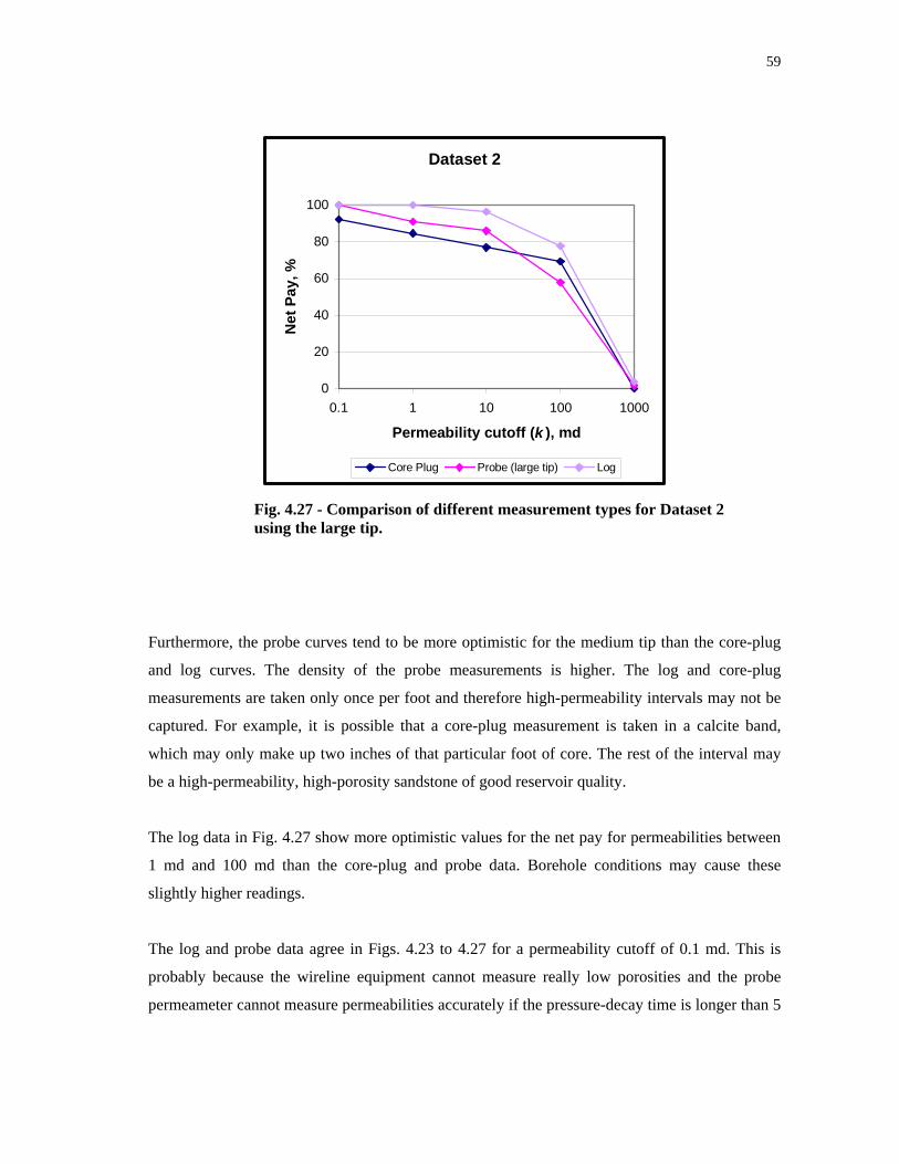
59

Dataset 2

0

20

40

60

80

100

0.1 1 10 100 1000

Permeability cutoff (k ), md

Net

Pay

, %

Core Plug Probe (large tip) Log

Fig. 4.27 - Comparison of different measurement types for Dataset 2 using the large tip.

Furthermore, the probe curves tend to be more optimistic for the medium tip than the core-plug

and log curves. The density of the probe measurements is higher. The log and core-plug

measurements are taken only once per foot and therefore high-permeability intervals may not be

captured. For example, it is possible that a core-plug measurement is taken in a calcite band,

which may only make up two inches of that particular foot of core. The rest of the interval may

be a high-permeability, high-porosity sandstone of good reservoir quality.

The log data in Fig. 4.27 show more optimistic values for the net pay for permeabilities between

1 md and 100 md than the core-plug and probe data. Borehole conditions may cause these

slightly higher readings.

The log and probe data agree in Figs. 4.23 to 4.27 for a permeability cutoff of 0.1 md. This is

probably because the wireline equipment cannot measure really low porosities and the probe

permeameter cannot measure permeabilities accurately if the pressure-decay time is longer than 5

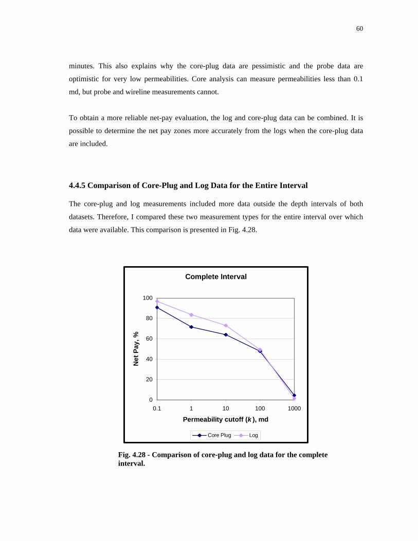
60

minutes. This also explains why the core-plug data are pessimistic and the probe data are

optimistic for very low permeabilities. Core analysis can measure permeabilities less than 0.1

md, but probe and wireline measurements cannot.

To obtain a more reliable net-pay evaluation, the log and core-plug data can be combined. It is

possible to determine the net pay zones more accurately from the logs when the core-plug data

are included.

4.4.5 Comparison of Core-Plug and Log Data for the Entire Interval

The core-plug and log measurements included more data outside the depth intervals of both

datasets. Therefore, I compared these two measurement types for the entire interval over which

data were available. This comparison is presented in Fig. 4.28.

Complete Interval

0

20

40

60

80

100

0.1 1 10 100 1000

Permeability cutoff (k ), md

Net

Pay

, %

Core Plug Log

Fig. 4.28 - Comparison of core-plug and log data for the complete interval.

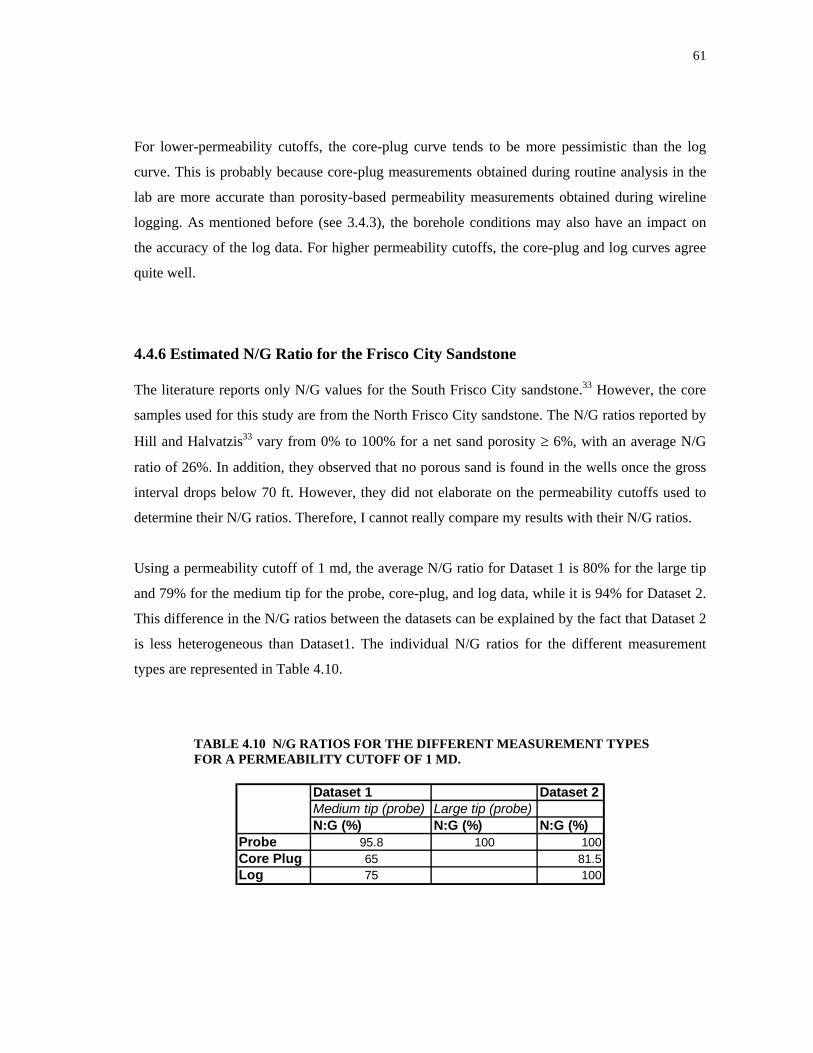
61

For lower-permeability cutoffs, the core-plug curve tends to be more pessimistic than the log

curve. This is probably because core-plug measurements obtained during routine analysis in the

lab are more accurate than porosity-based permeability measurements obtained during wireline

logging. As mentioned before (see 3.4.3), the borehole conditions may also have an impact on

the accuracy of the log data. For higher permeability cutoffs, the core-plug and log curves agree

quite well.

4.4.6 Estimated N/G Ratio for the Frisco City Sandstone

The literature reports only N/G values for the South Frisco City sandstone.33 However, the core

samples used for this study are from the North Frisco City sandstone. The N/G ratios reported by

Hill and Halvatzis33 vary from 0% to 100% for a net sand porosity ≥ 6%, with an average N/G

ratio of 26%. In addition, they observed that no porous sand is found in the wells once the gross

interval drops below 70 ft. However, they did not elaborate on the permeability cutoffs used to

determine their N/G ratios. Therefore, I cannot really compare my results with their N/G ratios.

Using a permeability cutoff of 1 md, the average N/G ratio for Dataset 1 is 80% for the large tip

and 79% for the medium tip for the probe, core-plug, and log data, while it is 94% for Dataset 2.

This difference in the N/G ratios between the datasets can be explained by the fact that Dataset 2

is less heterogeneous than Dataset1. The individual N/G ratios for the different measurement

types are represented in Table 4.10.

TABLE 4.10 N/G RATIOS FOR THE DIFFERENT MEASUREMENT TYPES FOR A PERMEABILITY CUTOFF OF 1 MD.

Dataset 1 Dataset 2Medium tip (probe) Large tip (probe)N:G (%) N:G (%) N:G (%)

Probe 95.8 100 100Core Plug 65 81.5Log 75 100

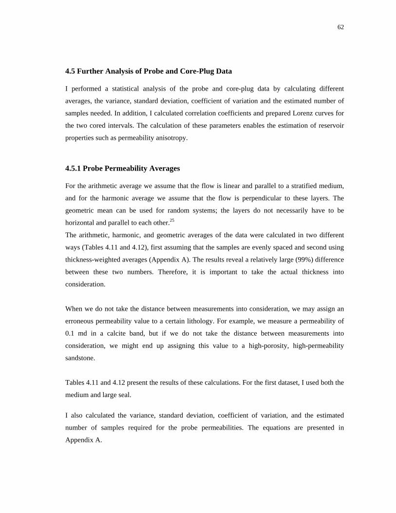
62

4.5 Further Analysis of Probe and Core-Plug Data

I performed a statistical analysis of the probe and core-plug data by calculating different

averages, the variance, standard deviation, coefficient of variation and the estimated number of

samples needed. In addition, I calculated correlation coefficients and prepared Lorenz curves for

the two cored intervals. The calculation of these parameters enables the estimation of reservoir

properties such as permeability anisotropy.

4.5.1 Probe Permeability Averages

For the arithmetic average we assume that the flow is linear and parallel to a stratified medium,

and for the harmonic average we assume that the flow is perpendicular to these layers. The

geometric mean can be used for random systems; the layers do not necessarily have to be

horizontal and parallel to each other.25

The arithmetic, harmonic, and geometric averages of the data were calculated in two different

ways (Tables 4.11 and 4.12), first assuming that the samples are evenly spaced and second using

thickness-weighted averages (Appendix A). The results reveal a relatively large (99%) difference

between these two numbers. Therefore, it is important to take the actual thickness into

consideration.

When we do not take the distance between measurements into consideration, we may assign an

erroneous permeability value to a certain lithology. For example, we measure a permeability of

0.1 md in a calcite band, but if we do not take the distance between measurements into

consideration, we might end up assigning this value to a high-porosity, high-permeability

sandstone.

Tables 4.11 and 4.12 present the results of these calculations. For the first dataset, I used both the

medium and large seal.

I also calculated the variance, standard deviation, coefficient of variation, and the estimated

number of samples required for the probe permeabilities. The equations are presented in

Appendix A.

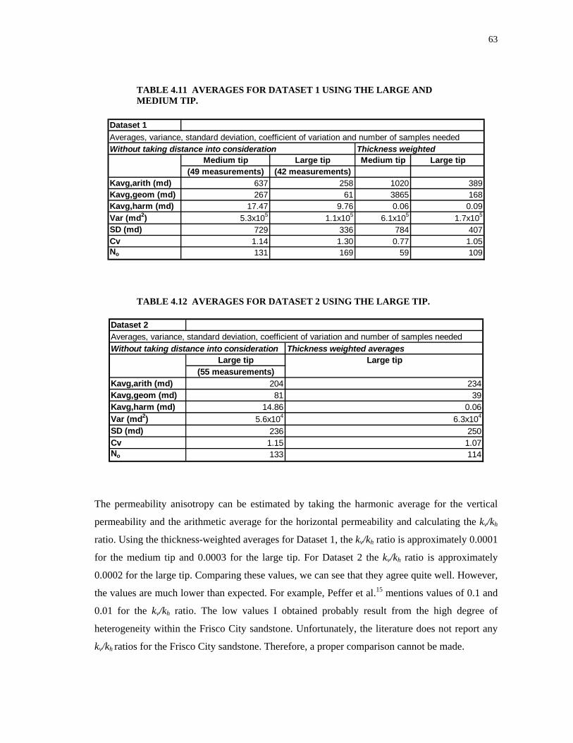
63

TABLE 4.11 AVERAGES FOR DATASET 1 USING THE LARGE AND MEDIUM TIP.

Dataset 1Averages, variance, standard deviation, coefficient of variation and number of samples neededWithout taking distance into consideration Thickness weighted

Medium tip Large tip Medium tip Large tip(49 measurements) (42 measurements)

Kavg,arith (md) 637 258 1020 389Kavg,geom (md) 267 61 3865 168Kavg,harm (md) 17.47 9.76 0.06 0.09Var (md2) 5.3x105 1.1x105 6.1x105 1.7x105

SD (md) 729 336 784 407Cv 1.14 1.30 0.77 1.05No 131 169 59 109

TABLE 4.12 AVERAGES FOR DATASET 2 USING THE LARGE TIP.

Dataset 2Averages, variance, standard deviation, coefficient of variation and number of samples neededWithout taking distance into consideration Thickness weighted averages

Large tip Large tip(55 measurements)

Kavg,arith (md) 204 234Kavg,geom (md) 81 39Kavg,harm (md) 14.86 0.06Var (md2) 5.6x104 6.3x104

SD (md) 236 250Cv 1.15 1.07No 133 114

The permeability anisotropy can be estimated by taking the harmonic average for the vertical

permeability and the arithmetic average for the horizontal permeability and calculating the kv/kh

ratio. Using the thickness-weighted averages for Dataset 1, the kv/kh ratio is approximately 0.0001

for the medium tip and 0.0003 for the large tip. For Dataset 2 the kv/kh ratio is approximately

0.0002 for the large tip. Comparing these values, we can see that they agree quite well. However,

the values are much lower than expected. For example, Peffer et al.15 mentions values of 0.1 and

0.01 for the kv/kh ratio. The low values I obtained probably result from the high degree of

heterogeneity within the Frisco City sandstone. Unfortunately, the literature does not report any

kv/kh ratios for the Frisco City sandstone. Therefore, a proper comparison cannot be made.

64

4.5.2 Probe Permeability Variabilities

As was the case with arithmetic and harmonic averages, the sample variance of the probe

permeabilities is sensitive to the appropriate vertical distances. The variance of Dataset 1 is

5.3x105 md2 for the medium tip and 1.1x105md2 for the large tip without taking the distance

between the samples into consideration. However, when I considered the thickness, the variance

changed to 6.1x105 md2 for the medium tip and 1.7x105 md2 for the large tip. For Dataset 2 the

variance is 5.6x104 md2 for the large tip without taking the distance between the samples into

consideration. The thickness-weighted variance for Dataset 2 is 6.3x104 md2. These numbers

indicate the dispersion or spread of the permeability about its mean.25 The variance of the

medium tip is slightly higher than the variance obtained with the large tip, probably because the

medium tip yielded higher permeabilities. Furthermore, the variance increased slightly when I

considered the distance between the samples. As mentioned before, when taking the distance

between the samples into consideration, one particular type of lithology can influence the

measurement more than another type.

The standard deviation or standard error, which is the positive square root of the variance, can be

used as a measure to judge how precise the estimate of the average permeability is.25 The

standard deviation for Dataset 1 is 729 md for the medium tip and 336 md for the large tip

without taking the distance between the samples into consideration. For Dataset 2 the standard

deviation is 236 md. The thickness-weighted standard deviations are 784 md, 407 md, and 250

md for the medium tip and large tip of Dataset 1 and the large tip of Dataset 2, respectively. The

thickness-weighted values are again slightly higher than the ones obtained without taking the

distance between the samples into consideration. The same reasoning is valid as for the variance.

Applying a 95% probability to these thickness-weighted standard deviations of the averages of

Dataset 1, the error in the arithmetic average can be ± 0.65 md for the medium tip, and ± 0.46 md

for the large tip. For Dataset 2 the error can be ± 0.17 md.

The coefficient of variation (Cv) describes the amount of variation in a population. In addition, it

can be used to compare and contrast variabilities of different facies.25 The coefficient of variation

without taking the distance between samples into consideration is 1.14 for the medium tip and

1.30 for the large tip for Dataset 1, and 1.15 for Dataset 2. The thickness-weighted coefficients of

variation are 0.77 and 1.05 respectively for the medium and large tip for Dataset 1, and 1.07 for

65

Dataset 2. According to Jensen et al.,25 a Cv of 0.77 to 1.30 can represent a heterogeneous

distributary/ tidal channel to a very heterogeneous fluvial, lateral-accretion sandstone. Indeed, the

Frisco City sandstone is very heterogeneous and fluvial and has a crossbedding structure.

The estimated number of samples needed (No) in a clastic reservoir can be calculated from the Cv

(see 3.1.1). The No without taking the distance between samples into consideration is 131 for the

medium tip and 169 for the large tip for Dataset 1, and 133 for Dataset 2. The thickness-weighted

Nos are 59 and 109 respectively for the medium and large tip for Dataset 1, and 114 for Dataset

2. The thickness-weighted No numbers are a little lower. As mentioned before, the lithology is

better represented when taking the sample spacing into consideration. This can explain the lower

number of samples required.

I took only 49 measurements with the medium tip and 42 with the large tip for Dataset 1. For

Dataset 2, I took 55 probe measurements. Only after the permeability data were analyzed could

the number of samples needed be estimated.

4.5.3 Core-Plug Averages

I also calculated the arithmetic, harmonic, and geometric averages, variance, standard deviation,

coefficient of variation, and the estimated number of samples needed for the core-plug data. The

calculations have been made without taking the distance into consideration and for the thickness-

weighted parameters. The results for both datasets are presented in Table 4.13, where we see that

only the geometric average changes considerably when taking the distance between samples into

consideration. Since the arithmetic average remains relatively constant, the variance, standard

deviation, coefficient of variation, and estimated number of samples needed do not change

dramatically. For example, the thickness-weighted Cv for Dataset 2 is 0.98, while it is 0.86 when

the sample spacing is not taken into consideration. The values remain relatively constant because

the sample density for the core plug is quite small and therefore the heterogeneity of the reservoir

is not really detected. The kv/kh ratios for the thickness-weighted core-plug data are 0.003 and

0.004 for Dataset 1 and Dataset 2 respectively.

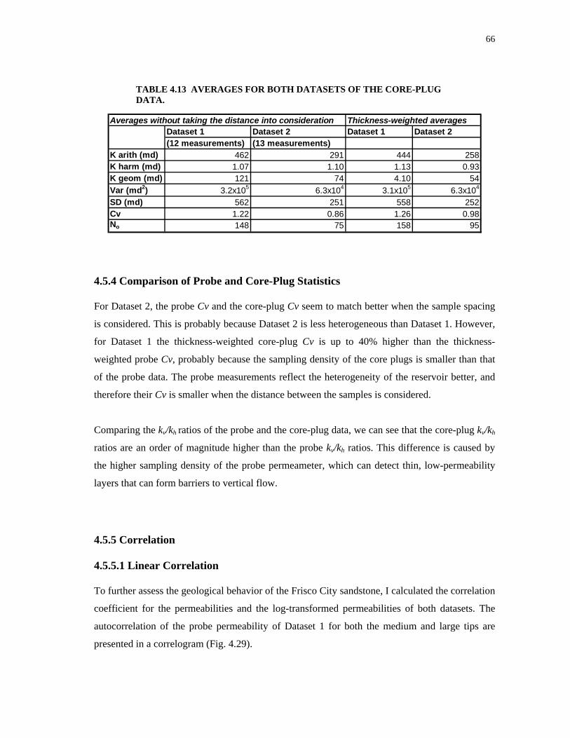
66

TABLE 4.13 AVERAGES FOR BOTH DATASETS OF THE CORE-PLUG DATA.

Averages without taking the distance into consideration Thickness-weighted averages

Dataset 1 Dataset 2 Dataset 1 Dataset 2(12 measurements) (13 measurements)

K arith (md) 462 291 444 258K harm (md) 1.07 1.10 1.13 0.93K geom (md) 121 74 4.10 54Var (md2) 3.2x105 6.3x104 3.1x105 6.3x104

SD (md) 562 251 558 252Cv 1.22 0.86 1.26 0.98No 148 75 158 95

4.5.4 Comparison of Probe and Core-Plug Statistics

For Dataset 2, the probe Cv and the core-plug Cv seem to match better when the sample spacing

is considered. This is probably because Dataset 2 is less heterogeneous than Dataset 1. However,

for Dataset 1 the thickness-weighted core-plug Cv is up to 40% higher than the thickness-

weighted probe Cv, probably because the sampling density of the core plugs is smaller than that

of the probe data. The probe measurements reflect the heterogeneity of the reservoir better, and

therefore their Cv is smaller when the distance between the samples is considered.

Comparing the kv/kh ratios of the probe and the core-plug data, we can see that the core-plug kv/kh

ratios are an order of magnitude higher than the probe kv/kh ratios. This difference is caused by

the higher sampling density of the probe permeameter, which can detect thin, low-permeability

layers that can form barriers to vertical flow.

4.5.5 Correlation

4.5.5.1 Linear Correlation

To further assess the geological behavior of the Frisco City sandstone, I calculated the correlation

coefficient for the permeabilities and the log-transformed permeabilities of both datasets. The

autocorrelation of the probe permeability of Dataset 1 for both the medium and large tips are

presented in a correlogram (Fig. 4.29).

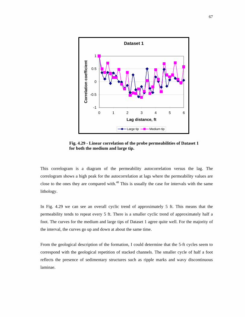
67

Dataset 1

-1

-0.5

0

0.5

1

0 1 2 3 4 5 6

Lag distance, ft

Cor

rela

tion

coef

ficie

nt

Large tip Medium tip

Fig. 4.29 - Linear correlation of the probe permeabilities of Dataset 1 for both the medium and large tip.

This correlogram is a diagram of the permeability autocorrelation versus the lag. The

correlogram shows a high peak for the autocorrelation at lags where the permeability values are

close to the ones they are compared with.48 This is usually the case for intervals with the same

lithology.

In Fig. 4.29 we can see an overall cyclic trend of approximately 5 ft. This means that the

permeability tends to repeat every 5 ft. There is a smaller cyclic trend of approximately half a

foot. The curves for the medium and large tips of Dataset 1 agree quite well. For the majority of

the interval, the curves go up and down at about the same time.

From the geological description of the formation, I could determine that the 5-ft cycles seem to

correspond with the geological repetition of stacked channels. The smaller cycle of half a foot

reflects the presence of sedimentary structures such as ripple marks and wavy discontinuous

laminae.

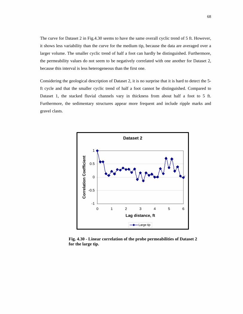
68

The curve for Dataset 2 in Fig.4.30 seems to have the same overall cyclic trend of 5 ft. However,

it shows less variability than the curve for the medium tip, because the data are averaged over a

larger volume. The smaller cyclic trend of half a foot can hardly be distinguished. Furthermore,

the permeability values do not seem to be negatively correlated with one another for Dataset 2,

because this interval is less heterogeneous than the first one.

Considering the geological description of Dataset 2, it is no surprise that it is hard to detect the 5-

ft cycle and that the smaller cyclic trend of half a foot cannot be distinguished. Compared to

Dataset 1, the stacked fluvial channels vary in thickness from about half a foot to 5 ft.

Furthermore, the sedimentary structures appear more frequent and include ripple marks and

gravel clasts.

Dataset 2

-1

-0.5

0

0.5

1

0 1 2 3 4 5 6

Lag distance, ft

Cor

rela

tion

Coe

ffici

ent

Large tip

Fig. 4.30 - Linear correlation of the probe permeabilities of Dataset 2 for the large tip.

69

4.5.5.2 Log-Transformed Permeability Correlation

The log-transformed permeability correlation curves in Figs. 4.31 and 4.32 exhibit the same trend

as those for the linear correlation. The overall cyclic trend is a little larger for Dataset 1 - about 6

ft. For Dataset 2 it seems to be slightly smaller - approximately 5 ft. Furthermore, Dataset 2

shows some negative associations for the log correlation. The smaller cyclic trend for Dataset 2

also varies in a range of about 3 in. to 1 ft.

Dataset 1 (Log k)

-1

-0.5

0

0.5

1

0 1 2 3 4 5 6

Lag distance, ft

Cor

rela

tion

coef

ficie

nt

Large tip Medium tip

Fig. 4.31 - Log-transformed correlation of the probe permeabilities of Dataset 1 for both the medium and large tip.

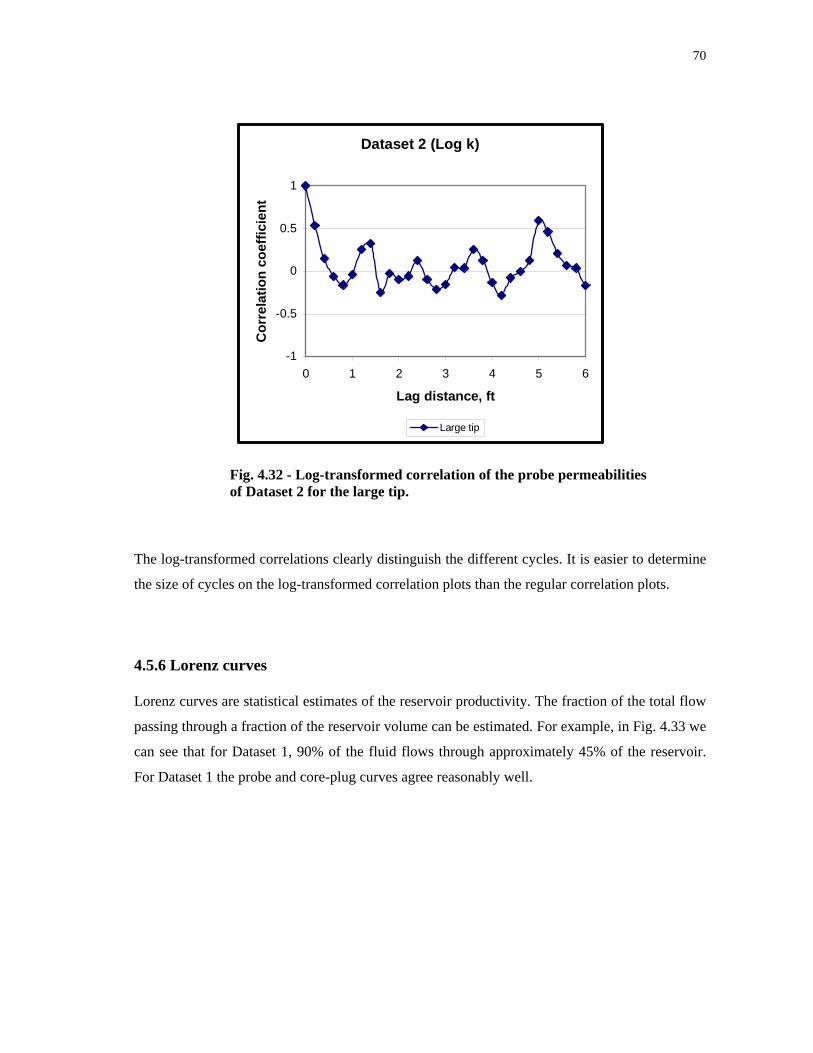
70

Dataset 2 (Log k)

-1

-0.5

0

0.5

1

0 1 2 3 4 5 6

Lag distance, ft

Cor

rela

tion

coef

ficie

nt

Large tip

Fig. 4.32 - Log-transformed correlation of the probe permeabilities of Dataset 2 for the large tip.

The log-transformed correlations clearly distinguish the different cycles. It is easier to determine

the size of cycles on the log-transformed correlation plots than the regular correlation plots.

4.5.6 Lorenz curves

Lorenz curves are statistical estimates of the reservoir productivity. The fraction of the total flow

passing through a fraction of the reservoir volume can be estimated. For example, in Fig. 4.33 we

can see that for Dataset 1, 90% of the fluid flows through approximately 45% of the reservoir.

For Dataset 1 the probe and core-plug curves agree reasonably well.

71

Dataset 1

0

0.2

0.4

0.6

0.8

1

0 0.2 0.4 0.6 0.8 1

Fraction of Total Storage Capacity (S)

Frac

tion

of T

otal

Flo

wC

apac

ity (F

)

Medium tip (probe) Large tip (probe) Core Plug

Fig. 4.33 - Lorenz curve for the probe data of Dataset 1 using both the medium and the large tip.

Dataset 2

0

0.2

0.4

0.6

0.8

1

0 0.2 0.4 0.6 0.8 1

Fraction of Total Storage Capacity (S)

Frac

tion

of T

otal

Flo

w

Cap

acity

(F)

Large tip (probe) Core Plug

Fig. 4.34 Lorenz curve for the probe data of Dataset 2 using the large tip.

72

In Fig. 4.34 we can see that for Dataset 2, 70% of the fluid flows through approximately 35% of

the reservoir. For Dataset 2, the probe curve tends to be more optimistic for higher permeability

values than the core-plug curve. As mentioned in 4.4.4, this may reflect higher sampling density

of the probe measurements. For the lower permeabilities, the probe and core-plug curves agree

better.

These values differ somewhat from the estimated N/G values obtained from the net pay analysis

for a permeability cutoff of 1 md. For example, the probe N/G ratio is 96 % for Dataset 1 and

80% for Dataset 2, whereas the Lorenz N/G ratio is 40% for both datasets. However, when we

determine the N/G ratio from the Lorenz curves, we do not apply a permeability cutoff. The

Lorenz N/G values compare better with the average N/G value of 26% for the South Frisco City

sandstone reported in the literature,33 although the authors did not indicate which permeability

cutoff value they applied to the N/G ratios.

4.6 Results and Implications for Other Reservoirs

For very heterogeneous reservoirs, it is advisable to determine the permeability anisotropy

because the presence of thin, low-permeability layers may form a barrier to vertical flow, and the

production forecast may be too optimistic if the kv/kh ratio is not considered.

Probe permeametry presents a cheap, efficient way to determine the net pay and permeability

anisotropy. Permeability measurements can be taken in a timely manner, without destruction of

the core samples. Furthermore, it is possible to cross check the geological model of the reservoir

by statistically analyzing the permeability data.

When log and core-plug data are available for a hydrocarbon reservoir, a comparison can be

made with the probe measurements. This leads to a more accurate petrophysical analysis. To

correct the depth shift of the log data, the core-plug data can be used since the core represents the

true depth. Another important issue is that the permeability cannot be determined from

conventional wireline logs. The probe and core-plug measurements can provide us with porosity

cutoffs to determine the log permeability cutoffs indirectly.

73

However, it is expensive to core every well. Therefore, when core plugs are not available, a

multiwell correlation can be made with the log data from other wells. When making this

correlation, it is important to take the reservoir geology into consideration. This method is not as

reliable and accurate as when core plugs are available, but it can be used to make an estimate of

the N/G ratio. For the Frisco City sandstone, there is a reasonably good agreement between the

log data and the probe and core-plug measurements. In very heterogeneous reservoirs, the log

data may be less accurate since measurements are only taken once per foot and thin, low-

permeability intervals may be missed.

In addition, acoustic logs can be used to indirectly determine the permeability from the porosity.

Another possibility is to obtain nuclear magnetic resonance logs from which the fluid

permeability can be calculated directly, instead of applying an indirect, porosity-based method.

For this heterogeneous reservoir the probe and core-plug Lorenz curves of Dataset 1 appear to

agree very well. Therefore, Lorenz curves may be useful for the N/G evaluation if data are

scarce, or when only log data are available.

74

CHAPTER V

SUMMARY

5.1 Conclusions

This study analyzed the different net pay definitions, evaluated net-pay estimation and the

permeability anisotropy in the Frisco City sandstone. Furthermore, the effect of different

measurements types such as probe, core-plug, and log measurements, and the effect of the

sampling strategy have also been explored. The following conclusions were drawn:

5.1.1 Conclusions Resulting from Literature Survey

1. There are several net-pay definitions. However, none of them is clear-cut and

unambiguous; they all contain a certain degree of uncertainty.

2. There are several ways to estimate the net pay, depending on the reason for

determination and available measurements. The static measurements do not

discriminate between hydrocarbon-bearing intervals and water-bearing intervals

and may therefore not be suitable for net-pay determination. The dynamic

measurements, which involve fluid flow and use a permeability cutoff, are better

suited for determining the net pay of a hydrocarbon reservoir.

3. For the production forecast of hydrocarbon reservoirs, it is important to determine

the producible net pay. With the estimated net pay, we can calculate the stock

tank oil in place (STOIP) and determine if the reservoir can be produced

economically.

4. The permeability anisotropy of a hydrocarbon reservoir should be considered

during the net-pay estimation. The kv/kh ratio of a heterogeneous reservoir is very

important since thin, low-permeability layers may be present. These layers can

form a barrier to vertical flow and the production forecast may be too optimistic if

these layers are not taken into consideration.

75

5. There are several ways to estimate permeability anisotropy depending on the time

and finances available. For example, a cost-effective, timely, and efficient way to

determine permeability anisotropy is to use the probe permeameter. The core

samples are not destroyed during analysis and as many measurements as

necessary can be taken.

5.1.2 Conclusions Specific to the Frisco City Sandstone

1. Geologically the two cored intervals are similar. Both consist of consolidated

sandstone interbedded with calcite cementing and thin shale layers.

2. The probe data and the lithological coefficient correlate well for the Frisco City

sandstone. The lithological coefficient is less than one for the higher-permeability

intervals and around either one or two for the lower-permeability values.

3. The net-pay variation depends on the measurement type. The probe

measurements represent the heterogeneity of the reservoir better than core-plug

measurements. With the probe we were able to identify the presence of thin shale

layers that were not detected by core-plug measurements.

4. A reduction in the sampling size did not really affect the probe, core-plug, or log

measurements. The net pay intervals did not change more than 17%.

5. The large tip gives more pessimistic values for the probe measurements than the

medium tip because the large tip averages values over a larger volume.

Therefore, it is advisable to use the medium tip for probe-permeameter

measurements.

6. The higher the permeability cutoff, the lower the net pay. The average probe net

pay for the Frisco City sandstone for a permeability cutoff of 1 md is 80% for

Dataset 1 and 94% for Dataset 2.

7. When comparing the probe, core-plug, and log curves for the net pay, the probe

curves tend to be more optimistic. This is caused by the higher sampling density

of the probe measurements. Log and core-plug measurements are taken only once

per foot and therefore high-permeability intervals may not be captured.

76

8. It is important to take the sample spacing into consideration when calculating

statistical parameters such as the average permeability for the Frisco City

sandstone. I detected a 99% difference in thickness-weighted averages and values

assuming an evenly spaced sample distribution. Furthermore, it is possible that

we assign an erroneous permeability value to a certain lithology if we assume

that the samples are evenly spaced.

9. The calculation of the coefficient of variation provided an indication of the

reservoir heterogeneity and geology. After comparing the thickness-weighted Cv

results to the visual description of the core and the geological description present

in the literature, I obtained the same geologic description of the two datasets.

10. The correlograms indicate that the geology in the Frisco City sandstone is

repeated about every 5 ft. These stacked fluvial channels contain sedimentary

structures such as ripple marks, which cause a smaller cycle for Dataset 1. Since

the sedimentary structures of Dataset 2 do not exhibit a regular trend, no smaller

cycle could be distinguished.

11. The Lorenz curves indicate that 90% of the fluid flows through 50% of the

reservoir for Dataset 1. For Dataset 2, 75% of the fluid flows through

approximately 40% of the reservoir.

12. The N/G data obtained from the net pay analysis and the Lorenz net pay agree

quite well for permeability cutoffs of 1 md and 10 md. Especially for the probe

net pay, the Lorenz values are relatively similar.

5.2 General Observations

In the petroleum industry, people have been trying to formulate net pay definitions for a long

time. However, today there is still no clear-cut definition that takes all the necessary parameters

into consideration. Therefore, it is time to adopt a general definition that can be adjusted

depending on the reservoir properties.

Determining the permeability anisotropy in heterogeneous reservoirs is very important. The

dynamic net pay depends on the permeability anisotropy of a reservoir and can be overestimated

77

if the barriers to flow in the vertical direction are not taken into consideration. If the permeability

anisotropy is high, the dynamic net pay may be small.

It is not surprising that the Frisco City sandstone exhibits a high degree of permeability

anisotropy. Both shales and crossbedding, two geologic features present in this formation, cause

heterogeneity on a scale that is usually smaller than the measuring device.

For the net pay and permeability anisotropy evaluation of a hydrocarbon reservoir, the probe

permeameter can be a cheap, useful device. Measurements can be taken without destruction of

the core samples in a timely and cost effective manner. Furthermore, it is possible to detect thin,

low-permeability intervals, which usually cannot be detected during routine core-plug analysis or

analysis of log data. Therefore, I would strongly recommend the performance of a probe analysis

on the reservoir intervals that have been determined as economically productive to reduce the

chances of a production forecast that is too optimistic.

5.3 Suggestions for Further Work

After finishing my research and data analysis several things remained that I would have liked to

perform. I suggest the following for further work:

• Measure the vertical permeability by taking vertical core plugs and compare the

results with the vertical permeability calculated from the harmonic average.

• Analyze data from nearby wells to determine the lateral extent of the lithology

and the permeability behavior.

• Create isopach maps for the net pay and determine the relationship between the

net pay, permeability anisotropy, and geology for the whole Frisco City field.

• Use log-based Lorenz curves as a permeability predictor and determine if there is

an agreement with the probe and core-plug Lorenz curves.

78

NOMENCLATURE

a = internal radius of the tip seal, cm

C = constant

Cv = coefficient of variation of a random variable

F = cumulative flow capacity

φ = porosity, %

G = geometrical factor

ka = air permeability, darcy

kavg = average permeability, md

kavg,arith = arithmetic average permeability, md

kavg,geom. = geometric average permeability, md

kavg,harm = harmonic average permeability, md

kv = vertical permeability, md

kh = horizontal permeability, md

MBVM = Magnetic Resonance Imaging Log bulk volume moveable

MBVI = Magnetic Resonance Imaging Log volume irreducible fluids

n = number of samples

No = estimated number of samples needed

Pi = measured flow pressure, atm

Po = atmospheric pressure, atm

Q = flow rate, cm3/sec

S = cumulative thickness, ft

SD = standard deviation or standard error, md

µ = air viscosity, cp

Var = variance, md2

79

REFERENCES

1. Tearpock, D.J. and Bischke, R.E.: Applied Subsurface Geological Mapping, first edition,

Prentice Hall PTR, Upper Saddle River, New Jersey (1991) 488-493.

2. Cobb, W.M. and Marek, F.J.: “Net Pay Determination for Primary and Waterflood

Depletion Mechanisms,” paper SPE 48952 presented at the 1998 SPE Annual Technical

Conference and Exhibition, New Orleans, 27-30 September.

3. Calhoun, J.C. Jr.: Fundamentals of Reservoir Engineering, revised edition, U. of

Oklahoma Press, Norman, Oklahoma (1960) 168-171.

4. Pirson, S.J.: Oil Reservoir Engineering, second edition, McGraw-Hill Book Co. Inc.,

New York (1958) 441-451.

5. Snyder, R.H.: “A Review of the Concepts and Methodology of Determining Net Pay”

paper SPE 3609 presented at the 1971 Annual Fall Meeting of the Society of Petroleum

Engineers of AIME, New Orleans, 3-6 October.

6. Petroleum Engineering Handbook, first edition, H.B. Bradley (ed.), SPE, Richardson,

Texas (1992).

7. Gaynor, G.C. and Sneider, R.M.: “Effective Pay Determination,” Development Geology

Reference Manual, D.M. Morton-Thompson and A.M. Woods (eds.), American

Association of Petroleum Geologists, Tulsa, Oklahoma, 286-288.

8. Craig, F.F.: The Reservoir Engineering Aspects of Waterflooding, first edition,

Monograph Series, SPE, Richardson, Texas (1993) 3, 48-57.

9. Lee, W.J.: Well Testing, first edition, SPE, New York (1982).

10. Doll, H.G.: “The Microlog – A New Electrical Logging Method for Detailed

Determination of Permeable Beds,” Petroleum Trans., AIME (1950) 189, 155-164.

11. Ball, L.D., Corbett, P.W.M., Jensen, J.L., and Lewis, J.J.M.: “The Role of Geology in the

Behavior and Choice of Permeability Predictors,” paper SPE 28447 presented at the

1994 SPE Annual Technical Conference and Exhibition, New Orleans, 25-28 September.

12. Petovello, B.G.: “Well Performance Evaluation by Production Logging,” Petr. Engr.

Intl. (1975) No. 8, 48.

13. Economides, M.J., Hill, A.D., and Ehlig-Economides, C.: Petroleum Production

Systems, first edition, Prentice Hall, Upper Saddle River, New Jersey (1994) 271-273.

80

14. Al-Harty, S.S., Jing, X.D., Marsden, J.R., and Dennis, J.W.: “Petrophysical Properties of

Sandstones Under True Triaxial Stresses I: Directional Transport Characteristics and

Pore Volume Change,” paper SPE 57287 presented at the 1999 SPE Asia Pacific

Improved Oil Recovery Conference, Kuala Lumpur, 25-26 October.

15. Peffer, J., O’Callaghan, A., and Pop, J.: “In-Situ Determination of Permeability

Anisotropy and its Vertical Distribution – A Case Study,” paper SPE 38942 presented at

the 1997 SPE Annual Technical Conference and Exhibition, San Antonio, Texas, 5-8

October.

16. Schlumberger, C., Schlumberger, M., and Leonardon, E.G.: “Some Observations

Concerning Electrical Measurements in Anisotropic Media and Their Interpretation,”

Petroleum Trans., AIME (1934) 110, 159-182.

17. Lake, L.W.: “The Origins of Anisotropy,” JPT (April 1998) 395.

18. Archer, J.S. and Wall, C.G.: Petroleum Engineering – Principles and Practice, first

edition, Graham and Trotman, Gaithersburg, Maryland (1986).

19. Economides, M.J., Watters, L.T., and Dunn-Norman, S.: Petroleum Well Construction,

first edition, John Wiley and Sons, Chichester, England (1998).

20. Thomas, S.D., Corbett, P.W.M., and Jensen, J.L.: “Upscaling Vertical Permeability

Within a Fluvio-Aeolian Reservoir,” paper presented at the Fourth International

Reservoir Characterization Technical Conference, Houston, 2-4 March 1997.

21. Wannell, M.J. and Morrison, S.J.: “Vertical Permeability Measurement in New

Reservoirs Using Tidal Pressure Changes,” paper SPE 20532 presented at the 1990 SPE

Annual Technical Conference and Exhibition, New Orleans, 23-25 September.

22. Head, E.L. and Pop, J.J.: “Reservoir Anisotropy Determination Using Multiple Probe

Pressures,” paper SPE 26048 presented at Western Regional Meeting, Anchorage, 26-28

May.

23. Georgi, D., Kasap, E., Tang, X., and Cheng, A.: “Permeability Profiles – Key to

Reservoir Management,” Petr. Engr. Intl. (1998) No. 6, 50.

24. Coates, G.R., Xiao, L., and Prammer, M.G.: NMR Logging, Principles and Applications,

first edition, Halliburton Energy Services, Houston (1999).

25. Jensen, J.L., Lake, L.W., Corbett, P.W.M., and Goggin, D.J.: Statistics for Petroleum

Engineers and Geoscientists, second edition, Elsevier, Amsterdam (2000).

81

26. Weber, K.J. and van Geuns, L.C.: “Framework for Constructing Clastic Reservoir

Simulation,” JPT (October 1990) 1248.

27. Montgomery, S.L., Baria, L.R., and Handford, C.R.: “Frisco City Sandstone: Upper

Jurassic Play in Southern Alabama,” AAPG Bull. (1997) 81, No. 10, 1595.

28. Baria, L.R. and Mink, R.M.: “ A Comparison of 2-D and 3-D Seismic Interpretation of

Monroeville Field, A Frisco City Sand Reservoir, Monroe County, Alabama,” GCAGS,

Special Publication (June 1998) 213.

29. Mann, S.D., Mink, R.M., Bearden, B.L., and Schneeflock Jr., R.D.: “ The Frisco City

Sand: A New Jurassic Reservoir in Southwest Alabama,” Trans., GCAGS (1989) 39,

195.

30. Stephenson, M.A., Cox, J.G., Harmount, M, and Bruno, L.: “A Subsurface Study of the

North Frisco City Field, Monroe County, Alabama,” Trans., GCAGS (1993) 43, 535.

31. Kugler, R.L. and Mink, R.M.: “Haynesville Sandstone Reservoirs in the Updip Jurassic

Trend of Alabama,” Trans., GCAGS (1994) 44, 764.

32. Mink, R.M. and Mancini, E.A.: “Upper Jurassic and Lower Cretaceous Oil Reservoirs of

the Updip Basement Structure Play: Southwest Alabama,” Trans., GCAGS (1995) 45,

441.

33. Hill, K.B. and Halvatzis, G.J.: “Sand Thickness Prediction from 3-D Seismic Data: A

Case Study of the Upper Jurassic Frisco City Sand of Southwest Alabama,” The Leading

Edge (September 2001) 950.

34. Hurst, A. and Goggin, D.: “Probe Permeametry: An Overview and Bibliography,” AAPG

Bull. (1995) 79, No. 3, 463.

35. Dreyer, T., Scheie, Å., and Walderhaug, O.: “Minipermeameter-Based Study of

Permeability Trends in Channel Sand Bodies,” AAPG Bull. (1990) 74, No. 4, 359.

36. Goggin, D.J.: “Probe Permeametry: Is it Worth the Effort?” Marine and Petroleum

Geology (1993) 10, No. 8, 299.

37. RP 40, Recommended Practices for Core Analysis, second edition, API, Washington, DC

(1998).

38. Hurst, A. and Rosvoll, K.: “Permeability Variations in Sandstones and Their

Relationship to Sedimentary Structures,” Reservoir Characterization II, Academic Press,

San Diego, California (1991) 166-196.

82

39. Sutherland, W.J., Halvorsen, C., Hurst, A., McPhee, C.A., Robertson, G. et al.:

“Recommended Practice for Probe Permeametry,” Marine and Petroleum Geology

(1993) 10, No. 8, 309.

40. Zheng, S., Corbett, P.W.M., and Stewart, G.: “Uncertainty in Well Test and Core

Permeability Analysis: A Case Study in Fluvial Channel Reservoirs, Northern North Sea,

Norway,” AAPG Bull. (2000) 84, No. 12, 1929.

41. Potocki, D.: “Resolving Differences Between Core and Welltest Permeability in Basal

Colorado Sandstones, Canada: The Role of Rock Heterogeneity, Relative Permeability

and Formation Damage,” paper SPE 71206 presented at the 2001 SPE Rocky Mountain

Petroleum Technology Conference, Keystone, Colorado, 21-23 May.

42. Jahn, F., Cook, M., and Graham, M.: Hydrocarbon Exploration and Production, first

edition,” Elsevier, Amsterdam (1998).

43. Mezghani, M., van Lingen, P., Cosentino, L., and Sengul, M.: “Conditioning

Geostatistical Models to Flow Meter Logs,” Paper SPE 65122 presented at the 2000 SPE

European Petroleum Conference, Paris, 24-25 October.

44. Weber, K.J.: “Computation of Initial Well Productivities in Aeolian Sandstone on the

Basis of a Geological Model, Leman Gas Field, U.K.,” Soc. of Economic Paleontologists

and Mineralogist Bull. (1987) 333-354.

45. Jensen, J.L.: “A Model for Small Scale Permeability Measurement with Applications to

Reservoir Description,” paper SPE 20265 presented at the 1990 SPE/DOE Symposium

on EOR, Tulsa, Oklahoma, 22-25 April.

46. Openhole Log Analysis and Formation Evaluation, EL1007, Halliburton, Houston

(1991).

47. Reservoir Characterization, Lake, L.W. and Carroll, H.B. Jr. (eds.), Academic Press

Inc., Orlando, Florida (1986).

48. Davis, J.C.: Statistics and Data Analysis in Geology, first edition, John Wiley & Sons,

New York (1973) 232-234.

83

APPENDIX A

EQUATIONS

1. Coates Equation:

⎥⎥⎦

⎤

⎢⎢⎣

⎡⎟⎠⎞

⎜⎝⎛•⎟

⎠⎞

⎜⎝⎛=

24

MBVIMBVM

Ck φ

2. SDR Model: 42

2 φgmaTk =

3. Averages of evenly spaced samples

Arithmetic average:

∑=

=n

iiavg k

nk

1

1

Harmonic average:

( ) ( )1

1

1 1 −

=

− ∑=n

iiavg k

nk

Geometric average:

( )nnavg kkkk ......21=

4. Thickness weighted averages

Arithmetic average:

∑∑

==i

n

iii

avg h

hk

nk 11

84

Harmonic average:

∑∑

==i

n

i i

i

avg hkh

nk 11

5. Variance of sample mean, kavg

( ) ⎟⎠

⎞⎜⎝

⎛= ∑

=

n

iiavg k

nVarkVar

1

1

6. Standard deviation of sample mean, kavg

( )avgkVarSD +=

7. Coefficient of variation of sample mean, kavg

arithavgV k

SDC,

=

8. Lorenz curves

∑

∑

=

== n

jj

i

jj

h

hS

1

1

∑

∑

=

== n

jjj

i

jjj

hk

hkF

1

1

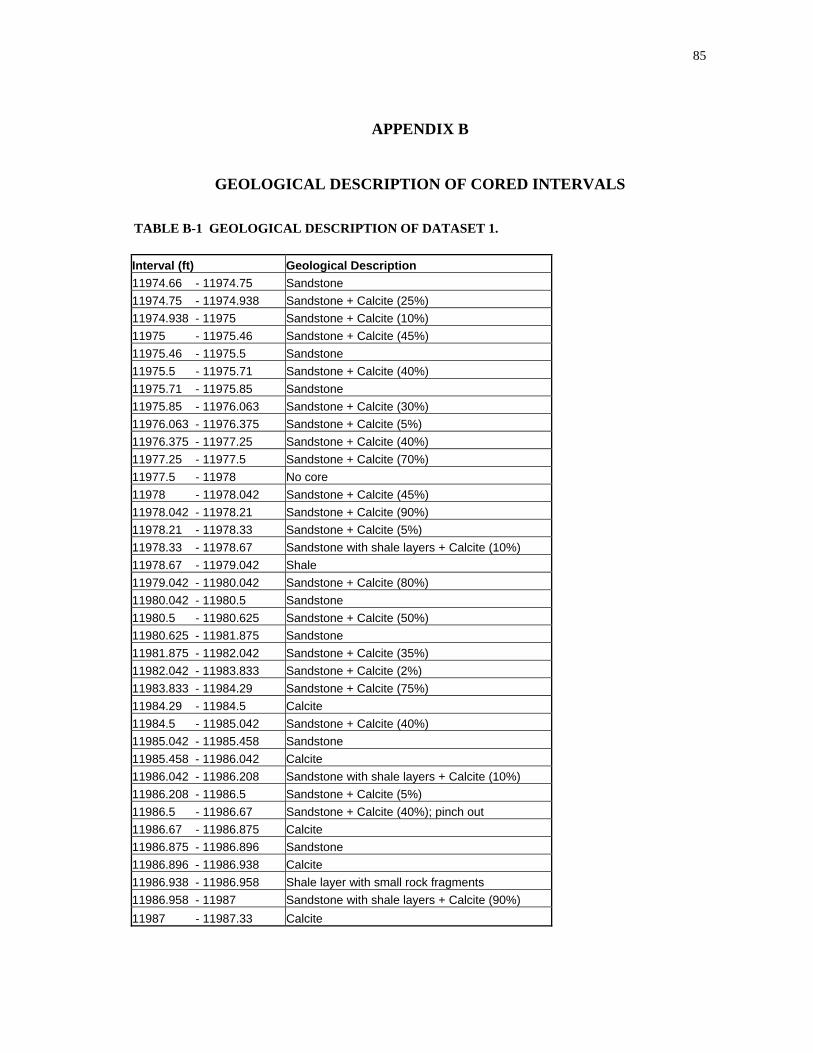
85

APPENDIX B

GEOLOGICAL DESCRIPTION OF CORED INTERVALS

TABLE B-1 GEOLOGICAL DESCRIPTION OF DATASET 1. Interval (ft) Geological Description 11974.66 - 11974.75 Sandstone 11974.75 - 11974.938 Sandstone + Calcite (25%) 11974.938 - 11975 Sandstone + Calcite (10%) 11975 - 11975.46 Sandstone + Calcite (45%) 11975.46 - 11975.5 Sandstone 11975.5 - 11975.71 Sandstone + Calcite (40%) 11975.71 - 11975.85 Sandstone 11975.85 - 11976.063 Sandstone + Calcite (30%) 11976.063 - 11976.375 Sandstone + Calcite (5%) 11976.375 - 11977.25 Sandstone + Calcite (40%) 11977.25 - 11977.5 Sandstone + Calcite (70%) 11977.5 - 11978 No core 11978 - 11978.042 Sandstone + Calcite (45%) 11978.042 - 11978.21 Sandstone + Calcite (90%) 11978.21 - 11978.33 Sandstone + Calcite (5%) 11978.33 - 11978.67 Sandstone with shale layers + Calcite (10%) 11978.67 - 11979.042 Shale 11979.042 - 11980.042 Sandstone + Calcite (80%) 11980.042 - 11980.5 Sandstone 11980.5 - 11980.625 Sandstone + Calcite (50%) 11980.625 - 11981.875 Sandstone 11981.875 - 11982.042 Sandstone + Calcite (35%) 11982.042 - 11983.833 Sandstone + Calcite (2%) 11983.833 - 11984.29 Sandstone + Calcite (75%) 11984.29 - 11984.5 Calcite 11984.5 - 11985.042 Sandstone + Calcite (40%) 11985.042 - 11985.458 Sandstone 11985.458 - 11986.042 Calcite 11986.042 - 11986.208 Sandstone with shale layers + Calcite (10%) 11986.208 - 11986.5 Sandstone + Calcite (5%) 11986.5 - 11986.67 Sandstone + Calcite (40%); pinch out 11986.67 - 11986.875 Calcite 11986.875 - 11986.896 Sandstone 11986.896 - 11986.938 Calcite 11986.938 - 11986.958 Shale layer with small rock fragments 11986.958 - 11987 Sandstone with shale layers + Calcite (90%) 11987 - 11987.33 Calcite

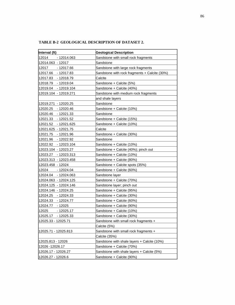
86

TABLE B-2 GEOLOGICAL DESCRIPTION OF DATASET 2.

Interval (ft) Geological Description 12014 - 12014.063 Sandstone with small rock fragments 12014.063 - 12017 Sandstone 12017 - 12017.66 Sandstone with large rock fragments 12017.66 - 12017.83 Sandstone with rock fragments + Calcite (30%) 12017.83 - 12018.79 Calcite 12018.79 - 12019.04 Sandstone + Calcite (5%) 12019.04 - 12019.104 Sandstone + Calcite (40%) 12019.104 - 12019.271 Sandstone with medium rock fragments and shale layers 12019.271 - 12020.25 Sandstone 12020.25 - 12020.46 Sandstone + Calcite (10%) 12020.46 - 12021.33 Sandstone 12021.33 - 12021.52 Sandstone + Calcite (15%) 12021.52 - 12021.625 Sandstone + Calcite (10%) 12021.625 - 12021.75 Calcite 12021.75 - 12021.96 Sandstone + Calcite (30%) 12021.96 - 12022.92 Sandstone 12022.92 - 12023.104 Sandstone + Calcite (10%) 12023.104 - 12023.27 Sandstone + Calcite (40%); pinch out 12023.27 - 12023.313 Sandstone + Calcite (10%) 12023.313 - 12023.458 Sandstone + Calcite (80%) 12023.458 - 12024 Sandstone + Calcite spots (35%) 12024 - 12024.04 Sandstone + Calcite (60%) 12024.04 - 12024.063 Sandstone layer 12024.063 - 12024.125 Sandstone + Calcite (70%) 12024.125 - 12024.146 Sandstone layer; pinch out 12024.146 - 12024.25 Sandstone + Calcite (95%) 12024.25 - 12024.33 Sandstone + Calcite (30%) 12024.33 - 12024.77 Sandstone + Calcite (60%) 12024.77 - 12025 Sandstone + Calcite (90%) 12025 - 12025.17 Sandstone + Calcite (10%) 12025.17 - 12025.33 Sandstone + Calcite (30%) 12025.33 - 12025.71 Sandstone with small rock fragments + Calcite (5%) 12025.71 - 12025.813 Sandstone with small rock fragments + Calcite (35%) 12025.813 - 12026 Sandstone with shale layers + Calcite (10%) 12026 -12026.17 Sandstone + Calcite (70%) 12026.17 - 12026.27 Sandstone with shale layers + Calcite (5%) 12026.27 - 12026.6 Sandstone + Calcite (90%)

87

VITA

Name: Janice Menke

Permanent Address: Balsemienstraat 4

Zorg & Hoop

Paramaribo

Suriname

Education: B.S., Geological Engineering

Anton de Kom University of Suriname

Paramaribo, Suriname

(November 1993 – December 1997)

M.S., Petroleum Engineering

(International Petroleum Management)

Texas A&M University

College Station, TX 77843-3116, U.S.A.

(August 1999 – May 2002)