Embed Size (px)
Citation preview
Chapter 1
GUSS:Solving Collections of Data RelatedModels within GAMS
Michael R. Bussieck, Michael C. Ferris, and Timo Lohmann
Abstract In many applications, optimization of a collection of problems isrequired where each problem is structurally the same, but in which some or allof the data defining the instance is updated. Such models are easily specifiedwithin modern modeling systems, but have often been slow to solve due tothe time needed to regenerate the instance, and the inability to use advancesolution information (such as basis factorizations) from previous solves as thecollection is processed. We describe a new language extension, GUSS, thatgathers data from different sources/symbols to define the collection of models(called scenarios), updates a base model instance with this scenario dataand solves the updated model instance and scatters the scenario results tosymbols in the GAMS database. We demonstrate the utility of this approachin three applications, namely data envelopment analysis, cross validation andstochastic dual dynamic programming. The language extensions are availablefor general use in all versions of GAMS starting with release 23.7.
1.1 Introduction
Algebraic modeling systems (such as GAMS, AMPL, AIMMS, etc) are a wellestablished methodology for solving broad classes of optimization problemsarising in a wide variety of application domains. These modeling systems takedata from a rich collection of sources including databases, spreadsheets, web
Michael R. BussieckGAMS Software GmbH, Cologne, e-mail: [email protected]
Michael C. Ferris
University of Wisconsin, Madison, Wisconsin e-mail: [email protected]
Timo LohmannGAMS Development Corp., Washington D.C., e-mail: [email protected]
1
2 Michael R. Bussieck, Michael C. Ferris, and Timo Lohmann
interfaces and simple text files and are able to process specific instantiationsof the often large and complex models using state of the art solution engines.
The purpose of this paper is to detail an extension of the GAMS modelingsystem that allows collections of models (parameterized exogenously by a setof samples or indices) to be described, instantiated and solved efficiently.
As a specific example, we consider the parametric optimization problemP(s) defined by:
minx∈X(s)
f(x; s) s.t. g(x; s) ≤ 0 (1.1)
where s ∈ S = {1, . . . ,K}. Note that each scenario s represents a differentproblem for which the optimization variable is x. The form of the constraintset as given above is simply for concreteness; equality constraints, range andbound constraints are trivial extensions of the above framework. Clearly theproblems P(s) are interlinked and we intend to show how such problems canbe easily specified within GAMS and detail one type of algorithmic extensionthat can exploit the nature of the linkage. Other extensions of GAMS allowsolves to be executed in parallel or using grid computing resources [6].
The paper is organized as follows. In Section 1.2 we outline the motiva-tion and design of the system for describing and solving P(s) and give someoverview of the available options. Section 1.3 gives three examples of the useof this methodology to the problems of data envelopment analysis (DEA - Sec-tion 1.3.1), cross validation for problems in machine learning (Section 1.3.2)and finally to stochastic dual dynamic programming (SDDP - Section 1.3.3).Note that in our description we will use the terms indexed, parameterized andscenario somewhat interchangeably. Furthermore we assume that the readerhas basic knowledge about the modeling language GAMS.
1.2 Design Methodology
One of the most important functions of GAMS is to build a model instancefrom the collection of equations (i.e. an optimization model defined by theGAMS keyword MODEL) and corresponding data (consisting of the content ofGAMS (sub)sets and parameters). Such a model instance is constructed orgenerated when the GAMS execution system executes a SOLVE statement.The generated model instance is passed to a solver which searches for a solu-tion of this model instance and returns status information, statistics, and a(primal and dual) solution of the model instance. After the solver terminates,GAMS brings back the solution into the GAMS database, i.e. it updates thelevel (.L) and marginal (.M) fields of variable and equation symbols used inthe model instance. Hence, the SOLVE statement can be interpreted as a com-plex operator against the GAMS database. The model instance generated bya SOLVE statement only lives during the execution of this one statement, andhence has no representation within the GAMS language. Moreover, its struc-
1 GUSS: Solving Collections of Data Related Models within GAMS 3
ture does fit the relational data model of GAMS. A model instance consistsof vectors of bounds and right hand sides, a sparse matrix representation ofthe Jacobian, a representation of the non-linear expressions that allow theefficient calculation of gradient vectors and Hessian matrices and so on.
This paper is concerned with solving collections of models that have similarstructure but modified data. As an example, consider a linear program of theform:
min cTx s.t. Ax ≥ b, ` ≤ x ≤ u.
The data in this problem is (A, b, c, `, u). Omitting some details, the followingcode could be used within GAMS to solve a collection of such linear programsin which each member of the collection has a different A matrix and lowerbound `:
1 Set i / ... /, j / ... /;
2 Parameter
3 A(i,j), b(i);
4 Variable
5 x(j), z, ...;
6 Equation
7 e(i), ...;
8 e(i).. sum(j, A(i,j)*x(j)) =g= b(i);
9 ...
10 model mymodel /all/;
11
12 Set s / s1*s10 /
13 Parameter
14 A_s(s,i,j) Scenario data
15 xlo_s(s,j) Scenario lower bound for variable x
16 xl_s(s,j) Scenario solution for x.l
17 em_s(s,i) Scenario solution for e.m;
18 Loop(s,
19 A(i,j) = A_s(s,i,j);
20 x.lo(j)= xlo_s(s,j);
21 solve mymodel min z using lp;
22 xl_s(s,j) = x.l(j);
23 em_s(s,i) = e.m(i);
24 );
Summarizing, we solve one particular model (mymodel) in a loop over s
with an unchanged model rim (i.e. the same individual variables and equa-tions) but with different model data and different bounds for the variables.The change in model data for a subsequent solve statement does not dependon the previous model solutions in the loop.
The purpose of this new Gather-Update-Solve-Scatter manager or shortGUSS is to provide syntax at the GAMS modeling level that makes an in-stance of a problem and allows the modeler limited access to treat that in-stance as an object, and to update portions of it iteratively. Specifically, weprovide syntax that gives a list of data changes to an instance, and allowsthese changes to be applied sequentially to the instance (which is then solved
4 Michael R. Bussieck, Michael C. Ferris, and Timo Lohmann
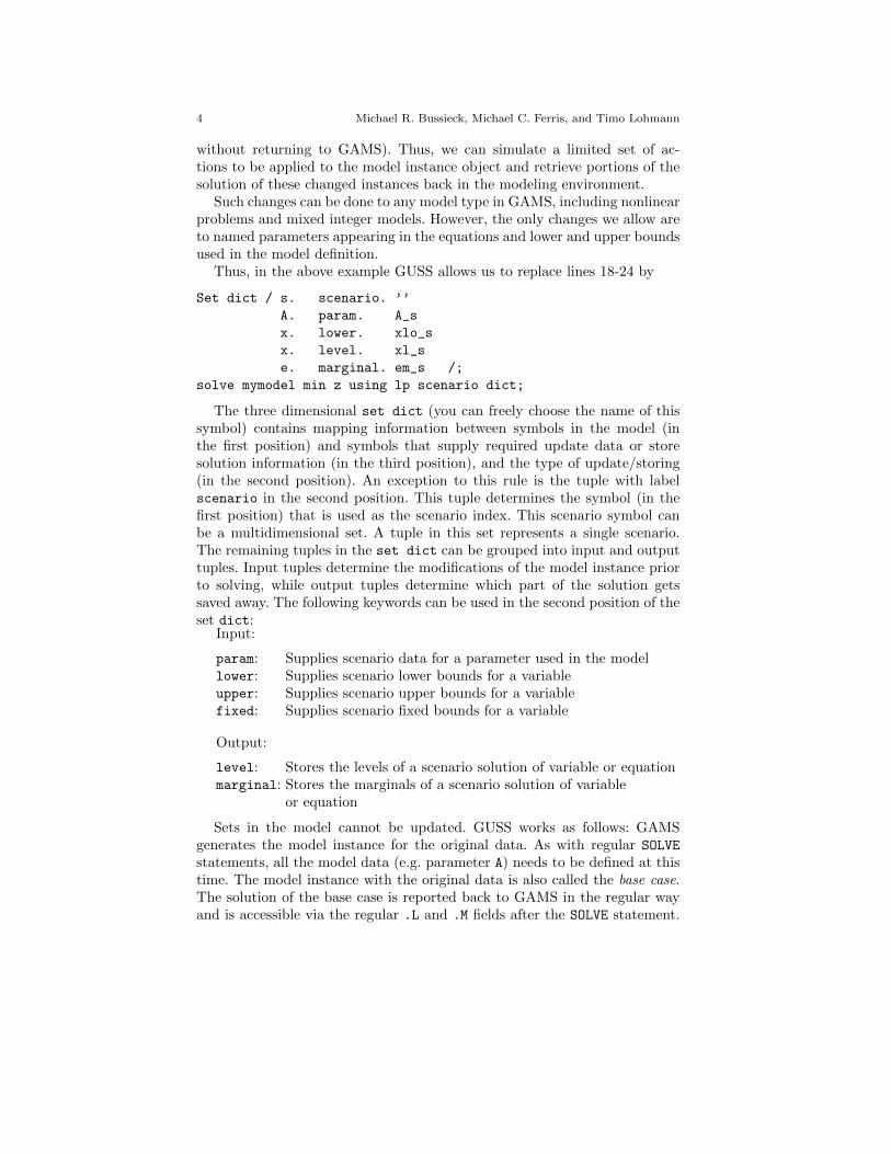
without returning to GAMS). Thus, we can simulate a limited set of ac-tions to be applied to the model instance object and retrieve portions of thesolution of these changed instances back in the modeling environment.
Such changes can be done to any model type in GAMS, including nonlinearproblems and mixed integer models. However, the only changes we allow areto named parameters appearing in the equations and lower and upper boundsused in the model definition.
Thus, in the above example GUSS allows us to replace lines 18-24 by
Set dict / s. scenario. ’’
A. param. A_s
x. lower. xlo_s
x. level. xl_s
e. marginal. em_s /;
solve mymodel min z using lp scenario dict;
The three dimensional set dict (you can freely choose the name of thissymbol) contains mapping information between symbols in the model (inthe first position) and symbols that supply required update data or storesolution information (in the third position), and the type of update/storing(in the second position). An exception to this rule is the tuple with labelscenario in the second position. This tuple determines the symbol (in thefirst position) that is used as the scenario index. This scenario symbol canbe a multidimensional set. A tuple in this set represents a single scenario.The remaining tuples in the set dict can be grouped into input and outputtuples. Input tuples determine the modifications of the model instance priorto solving, while output tuples determine which part of the solution getssaved away. The following keywords can be used in the second position of theset dict:
Input:
param: Supplies scenario data for a parameter used in the modellower: Supplies scenario lower bounds for a variableupper: Supplies scenario upper bounds for a variablefixed: Supplies scenario fixed bounds for a variable
Output:
level: Stores the levels of a scenario solution of variable or equationmarginal: Stores the marginals of a scenario solution of variable
or equation
Sets in the model cannot be updated. GUSS works as follows: GAMSgenerates the model instance for the original data. As with regular SOLVE
statements, all the model data (e.g. parameter A) needs to be defined at thistime. The model instance with the original data is also called the base case.The solution of the base case is reported back to GAMS in the regular wayand is accessible via the regular .L and .M fields after the SOLVE statement.
1 GUSS: Solving Collections of Data Related Models within GAMS 5
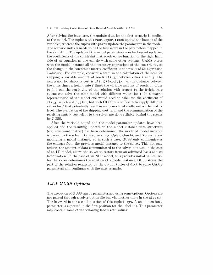
After solving the base case, the update data for the first scenario is appliedto the model. The tuples with lower, upper, fixed update the bounds of thevariables, whereas the tuples with param update the parameters in the model.The scenario index k needs to be the first index in the parameters mapped inthe set dict. The update of the model parameters goes far beyond updatingthe coefficients of the constraint matrix/objective function or the right handside of an equation as one can do with some other systems. GAMS storeswith the model instance all the necessary expressions of the constraints, sothe change in the constraint matrix coefficient is the result of an expressionevaluation. For example, consider a term in the calculation of the cost forshipping a variable amount of goods x(i,j) between cities i and j. Theexpression for shipping cost is d(i,j)*f*x(i,j), i.e. the distance betweenthe cities times a freight rate f times the variable amount of goods. In orderto find out the sensitivity of the solution with respect to the freight ratef, one can solve the same model with different values for f. In a matrixrepresentation of the model one would need to calculate the coefficient ofx(i,j) which is d(i,j)*f, but with GUSS it is sufficient to supply differentvalues for f that potentially result in many modified coefficient on the matrixlevel. The evaluation of the shipping cost term and the communication of theresulting matrix coefficient to the solver are done reliably behind the scenesby GUSS.
After the variable bound and the model parameter updates have beenapplied and the resulting updates to the model instance data structures(e.g. constraint matrix) has been determined, the modified model instanceis passed to the solver. Some solvers (e.g. Cplex, Gurobi, and Xpress) allowmodifying a model instance. So in such a case, GUSS only communicatesthe changes from the previous model instance to the solver. This not onlyreduces the amount of data communicated to the solver, but also, in the caseof an LP model, allows the solver to restart from an advanced basis and itsfactorization. In the case of an NLP model, this provides initial values. Af-ter the solver determines the solution of a model instance, GUSS stores thepart of the solution requested by the output tuples of dict to some GAMSparameters and continues with the next scenario.
1.2.1 GUSS Options
The execution of GUSS can be parameterized using some options. Options arenot passed through a solver option file but via another tuple in the dict set.The keyword in the second position of this tuple is opt. A one dimensionalparameter is expected in the first position (or the label ’’). This parametermay contain some of the following labels with values:
6 Michael R. Bussieck, Michael C. Ferris, and Timo Lohmann
OptfileInit: Option file number for the first solveOptfile: Option file number for subsequent solvesLogOption: Determines amount of log output:
0 - Moderate log (default)1 - Minimal log2 - Detailed log
SkipBaseCase: Switch for solving the base case (0 solves the base case)UpdateType: Scenario update mechanism:
0 - Set everything to zero and apply changes (default)1 - Reestablish base case and apply changes2 - Build on top of last scenario and apply changes
RestartType: Determines restart point for the scenarios0 - Restart from last solution (default)1 - Restart from solution of base case2 - Restart from input point
For the example model above the UpdateType setting would mean:
UpdateType=0: loop(s, A(i,j) = A_s(s,i,j))
UpdateType=1: loop(s, A(i,j) = A_base(i,j);
A(i,j) $= A_s(s,i,j))
UpdateType=2: loop(s, A(i,j) $= A_s(s,i,j))
The option SkipBaseCase=1 allows to skip the base case. This means onlythe scenarios are solved and there is no solution reported back to GAMSin the traditional way. The third position in the opt-tuple can contain aparameter for storing the scenario solution status information, e.g. modeland solve status, or needs to have the label ’’. The labels to store solutionstatus information must be known to GAMS, so one needs to declare a setwith such labels. The following solution status labels can be reported:
domusd iterusd objest nodusd modelstat numnopt
numinfes objval rescalc resderiv resin resout
resusd robj solvestat suminfes
The following example shows how to use some of the GUSS options andthe use of a parameter to store some solution status information:
Set h solution headers / modelstat, solvestat, objval /;
Parameter
o / SkipBaseCase 1, UpdateType 1, Optfile 1 /
r_s(s,h) Solution status report;
Set dict / s. scenario. ’’
o. opt. r_s
a. param. a_s
x. lower. xlo_s
x. level. xl_s
e. marginal. em_s /;
solve mymodel min z using lp scenario dict;
1 GUSS: Solving Collections of Data Related Models within GAMS 7
1.2.2 Implementation Details
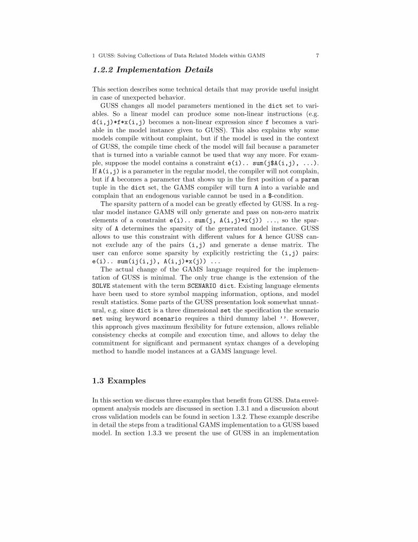
This section describes some technical details that may provide useful insightin case of unexpected behavior.
GUSS changes all model parameters mentioned in the dict set to vari-ables. So a linear model can produce some non-linear instructions (e.g.d(i,j)*f*x(i,j) becomes a non-linear expression since f becomes a vari-able in the model instance given to GUSS). This also explains why somemodels compile without complaint, but if the model is used in the contextof GUSS, the compile time check of the model will fail because a parameterthat is turned into a variable cannot be used that way any more. For exam-ple, suppose the model contains a constraint e(i).. sum(j$A(i,j), ...).If A(i,j) is a parameter in the regular model, the compiler will not complain,but if A becomes a parameter that shows up in the first position of a param
tuple in the dict set, the GAMS compiler will turn A into a variable andcomplain that an endogenous variable cannot be used in a $-condition.
The sparsity pattern of a model can be greatly effected by GUSS. In a reg-ular model instance GAMS will only generate and pass on non-zero matrixelements of a constraint e(i).. sum(j, A(i,j)*x(j)) ..., so the spar-sity of A determines the sparsity of the generated model instance. GUSSallows to use this constraint with different values for A hence GUSS can-not exclude any of the pairs (i,j) and generate a dense matrix. Theuser can enforce some sparsity by explicitly restricting the (i,j) pairs:e(i).. sum(ij(i,j), A(i,j)*x(j)) ...
The actual change of the GAMS language required for the implemen-tation of GUSS is minimal. The only true change is the extension of theSOLVE statement with the term SCENARIO dict. Existing language elementshave been used to store symbol mapping information, options, and modelresult statistics. Some parts of the GUSS presentation look somewhat unnat-ural, e.g. since dict is a three dimensional set the specification the scenarioset using keyword scenario requires a third dummy label ’’. However,this approach gives maximum flexibility for future extension, allows reliableconsistency checks at compile and execution time, and allows to delay thecommitment for significant and permanent syntax changes of a developingmethod to handle model instances at a GAMS language level.
1.3 Examples
In this section we discuss three examples that benefit from GUSS. Data envel-opment analysis models are discussed in section 1.3.1 and a discussion aboutcross validation models can be found in section 1.3.2. These example describein detail the steps from a traditional GAMS implementation to a GUSS basedmodel. In section 1.3.3 we present the use of GUSS in an implementation
8 Michael R. Bussieck, Michael C. Ferris, and Timo Lohmann
of the stochastic dual dynamic program. As many other decomposition al-gorithms SDDP requires the solution of many closely related mathematicaloptimization problems. We discuss in detail the savings in running time whenusing GUSS compared to a traditional GAMS implementation and even animplementation based on a native solver interface.
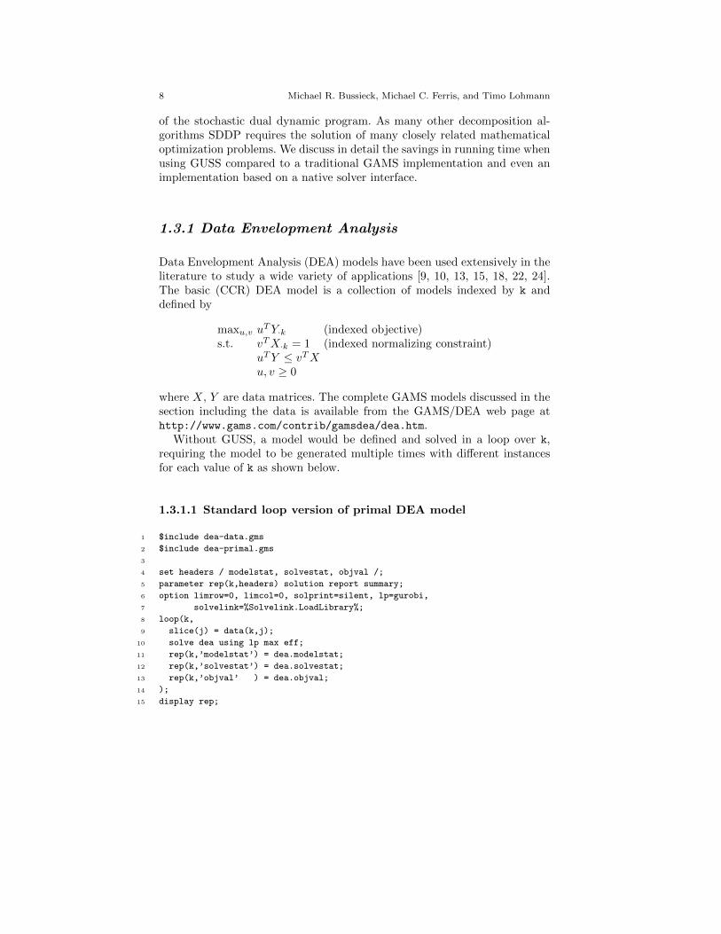
1.3.1 Data Envelopment Analysis
Data Envelopment Analysis (DEA) models have been used extensively in theliterature to study a wide variety of applications [9, 10, 13, 15, 18, 22, 24].The basic (CCR) DEA model is a collection of models indexed by k anddefined by
maxu,v uTY·k (indexed objective)
s.t. vTX·k = 1 (indexed normalizing constraint)uTY ≤ vTXu, v ≥ 0
where X, Y are data matrices. The complete GAMS models discussed in thesection including the data is available from the GAMS/DEA web page athttp://www.gams.com/contrib/gamsdea/dea.htm.
Without GUSS, a model would be defined and solved in a loop over k,requiring the model to be generated multiple times with different instancesfor each value of k as shown below.
1.3.1.1 Standard loop version of primal DEA model
1 $include dea-data.gms
2 $include dea-primal.gms
3
4 set headers / modelstat, solvestat, objval /;
5 parameter rep(k,headers) solution report summary;
6 option limrow=0, limcol=0, solprint=silent, lp=gurobi,
7 solvelink=%Solvelink.LoadLibrary%;
8 loop(k,
9 slice(j) = data(k,j);
10 solve dea using lp max eff;
11 rep(k,’modelstat’) = dea.modelstat;
12 rep(k,’solvestat’) = dea.solvestat;
13 rep(k,’objval’ ) = dea.objval;
14 );
15 display rep;
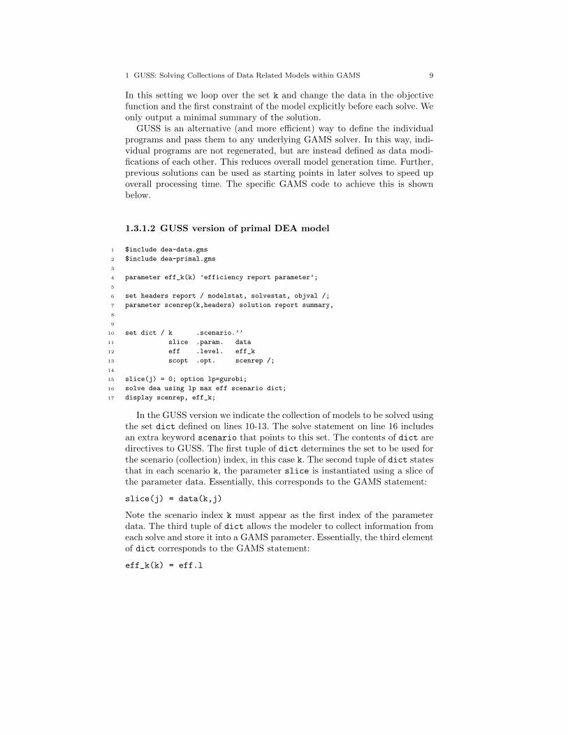
1 GUSS: Solving Collections of Data Related Models within GAMS 9
In this setting we loop over the set k and change the data in the objectivefunction and the first constraint of the model explicitly before each solve. Weonly output a minimal summary of the solution.
GUSS is an alternative (and more efficient) way to define the individualprograms and pass them to any underlying GAMS solver. In this way, indi-vidual programs are not regenerated, but are instead defined as data modi-fications of each other. This reduces overall model generation time. Further,previous solutions can be used as starting points in later solves to speed upoverall processing time. The specific GAMS code to achieve this is shownbelow.
1.3.1.2 GUSS version of primal DEA model
1 $include dea-data.gms
2 $include dea-primal.gms
3
4 parameter eff_k(k) ’efficiency report parameter’;
5
6 set headers report / modelstat, solvestat, objval /;
7 parameter scenrep(k,headers) solution report summary,
8
9
10 set dict / k .scenario.’’
11 slice .param. data
12 eff .level. eff_k
13 scopt .opt. scenrep /;
14
15 slice(j) = 0; option lp=gurobi;
16 solve dea using lp max eff scenario dict;
17 display scenrep, eff_k;
In the GUSS version we indicate the collection of models to be solved usingthe set dict defined on lines 10-13. The solve statement on line 16 includesan extra keyword scenario that points to this set. The contents of dict aredirectives to GUSS. The first tuple of dict determines the set to be used forthe scenario (collection) index, in this case k. The second tuple of dict statesthat in each scenario k, the parameter slice is instantiated using a slice ofthe parameter data. Essentially, this corresponds to the GAMS statement:
slice(j) = data(k,j)
Note the scenario index k must appear as the first index of the parameterdata. The third tuple of dict allows the modeler to collect information fromeach solve and store it into a GAMS parameter. Essentially, the third elementof dict corresponds to the GAMS statement:
eff_k(k) = eff.l
10 Michael R. Bussieck, Michael C. Ferris, and Timo Lohmann
that gets executed immediately after the solve of scenario k. GUSS options(scopt) and a parameter to store model statistics (scenrep) are given in thelast tuple of dict indicated by the keyword opt.
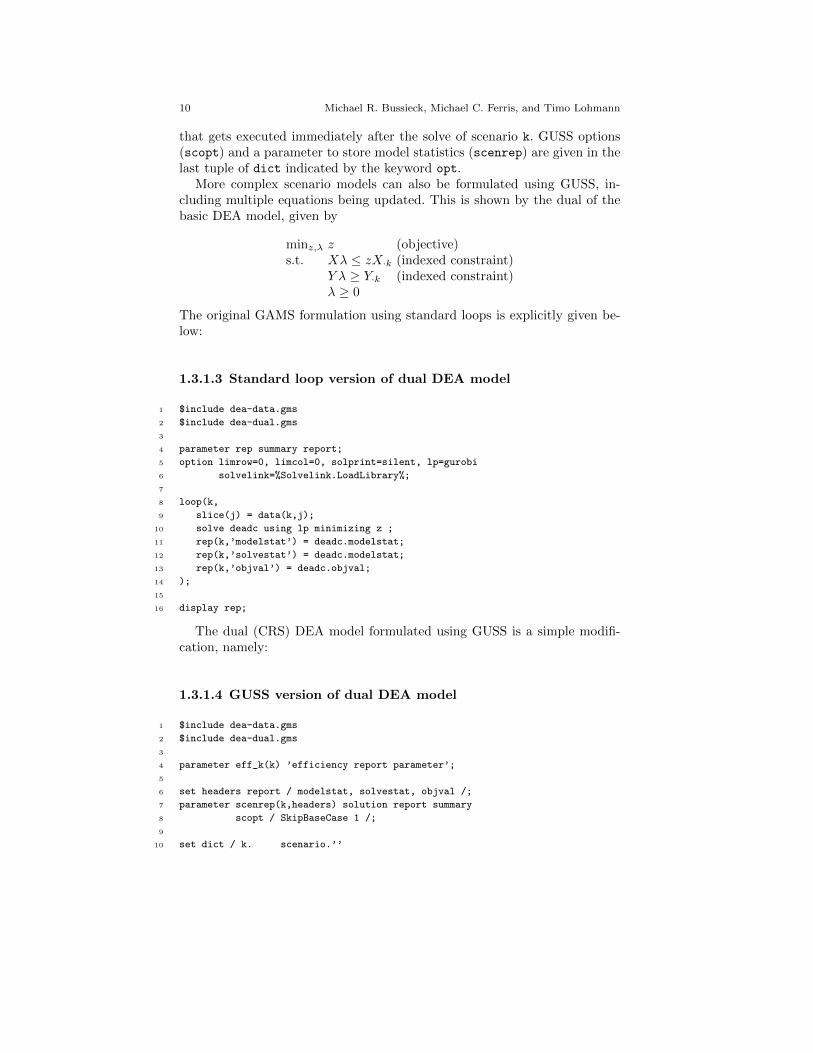
More complex scenario models can also be formulated using GUSS, in-cluding multiple equations being updated. This is shown by the dual of thebasic DEA model, given by
minz,λ z (objective)s.t. Xλ ≤ zX·k (indexed constraint)
Y λ ≥ Y·k (indexed constraint)λ ≥ 0
The original GAMS formulation using standard loops is explicitly given be-low:
1.3.1.3 Standard loop version of dual DEA model
1 $include dea-data.gms
2 $include dea-dual.gms
3
4 parameter rep summary report;
5 option limrow=0, limcol=0, solprint=silent, lp=gurobi
6 solvelink=%Solvelink.LoadLibrary%;
7
8 loop(k,
9 slice(j) = data(k,j);
10 solve deadc using lp minimizing z ;
11 rep(k,’modelstat’) = deadc.modelstat;
12 rep(k,’solvestat’) = deadc.modelstat;
13 rep(k,’objval’) = deadc.objval;
14 );
15
16 display rep;
The dual (CRS) DEA model formulated using GUSS is a simple modifi-cation, namely:
1.3.1.4 GUSS version of dual DEA model
1 $include dea-data.gms
2 $include dea-dual.gms
3
4 parameter eff_k(k) ’efficiency report parameter’;
5
6 set headers report / modelstat, solvestat, objval /;
7 parameter scenrep(k,headers) solution report summary
8 scopt / SkipBaseCase 1 /;
9
10 set dict / k. scenario.’’
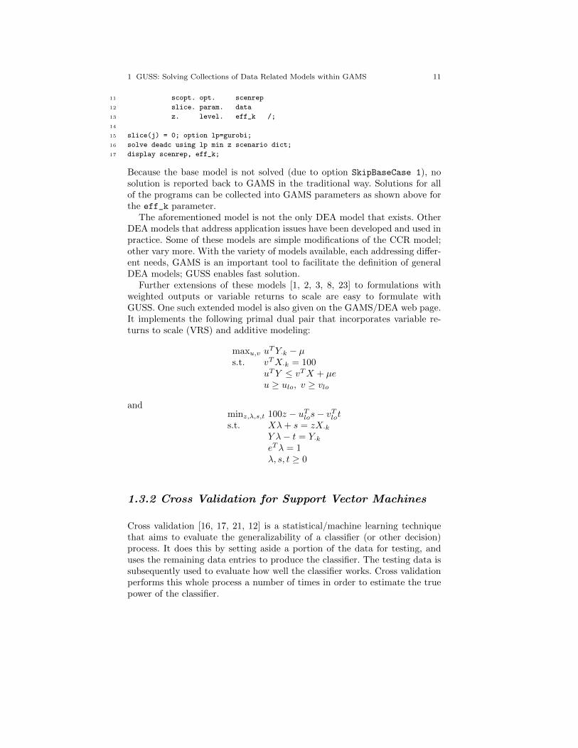
1 GUSS: Solving Collections of Data Related Models within GAMS 11
11 scopt. opt. scenrep
12 slice. param. data
13 z. level. eff_k /;
14
15 slice(j) = 0; option lp=gurobi;
16 solve deadc using lp min z scenario dict;
17 display scenrep, eff_k;
Because the base model is not solved (due to option SkipBaseCase 1), nosolution is reported back to GAMS in the traditional way. Solutions for allof the programs can be collected into GAMS parameters as shown above forthe eff_k parameter.
The aforementioned model is not the only DEA model that exists. OtherDEA models that address application issues have been developed and used inpractice. Some of these models are simple modifications of the CCR model;other vary more. With the variety of models available, each addressing differ-ent needs, GAMS is an important tool to facilitate the definition of generalDEA models; GUSS enables fast solution.
Further extensions of these models [1, 2, 3, 8, 23] to formulations withweighted outputs or variable returns to scale are easy to formulate withGUSS. One such extended model is also given on the GAMS/DEA web page.It implements the following primal dual pair that incorporates variable re-turns to scale (VRS) and additive modeling:
maxu,v uTY·k − µ
s.t. vTX·k = 100uTY ≤ vTX + µeu ≥ ulo, v ≥ vlo
andminz,λ,s,t 100z − uTlos− vTlots.t. Xλ+ s = zX·k
Y λ− t = Y·keTλ = 1λ, s, t ≥ 0
1.3.2 Cross Validation for Support Vector Machines
Cross validation [16, 17, 21, 12] is a statistical/machine learning techniquethat aims to evaluate the generalizability of a classifier (or other decision)process. It does this by setting aside a portion of the data for testing, anduses the remaining data entries to produce the classifier. The testing data issubsequently used to evaluate how well the classifier works. Cross validationperforms this whole process a number of times in order to estimate the truepower of the classifier.
12 Michael R. Bussieck, Michael C. Ferris, and Timo Lohmann
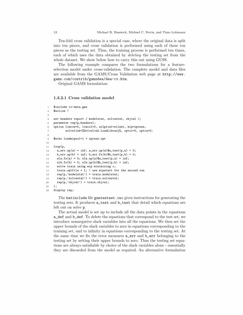
Ten-fold cross validation is a special case, where the original data is splitinto ten pieces, and cross validation is performed using each of these tenpieces as the testing set. Thus, the training process is performed ten times,each of which uses the data obtained by deleting the testing set from thewhole dataset. We show below how to carry this out using GUSS.
The following example compares the two formulations for a feature-selection model under cross-validation. The complete model and data filesare available from the GAMS/Cross Validation web page at http://www.
gams.com/contrib/gamsdea/dea-cv.htm.Original GAMS formulation:
1.3.2.1 Cross validation model
1 $include cv-data.gms
2 $eolcom !
3
4 set headers report / modelstat, solvestat, objval /;
5 parameter rep(p,headers);
6 option limrow=0, limcol=0, solprint=silent, mip=xpress,
7 solvelink=%Solvelink.LoadLibrary%, optcr=0, optca=0;
8
9 $echo loadmipsol=1 > xpress.opt
10
11 loop(p,
12 a_err.up(a) = inf; a_err.up(a)$a_test(p,a) = 0;
13 b_err.up(b) = inf; b_err.fx(b)$b_test(p,b) = 0;
14 sla.fx(a) = 0; sla.up(a)$a_test(p,a) = inf;
15 slb.fx(b) = 0; slb.up(b)$b_test(p,b) = inf;
16 solve train using mip minimizing c;
17 train.optfile = 1; ! use mipstart for the second run
18 rep(p,’modelstat’) = train.modelstat;
19 rep(p,’solvestat’) = train.solvestat;
20 rep(p,’objval’) = train.objval;
21 );
22 display rep;
The batinclude file gentestset.inc gives instructions for generating thetesting sets. It produces a_test and b_test that detail which equations areleft out on solve p.
The actual model is set up to include all the data points in the equationsa_def and b_def. To delete the equations that correspond to the test set, weintroduce nonnegative slack variables into all the equations. We then set theupper bounds of the slack variables to zero in equations corresponding to thetraining set, and to infinity in equations corresponding to the testing set. Atthe same time we fix the error measures a_err and b_err belonging to thetesting set by setting their upper bounds to zero. Thus the testing set equa-tions are always satisfiable by choice of the slack variables alone - essentiallythey are discarded from the model as required. An alternative formulation
1 GUSS: Solving Collections of Data Related Models within GAMS 13
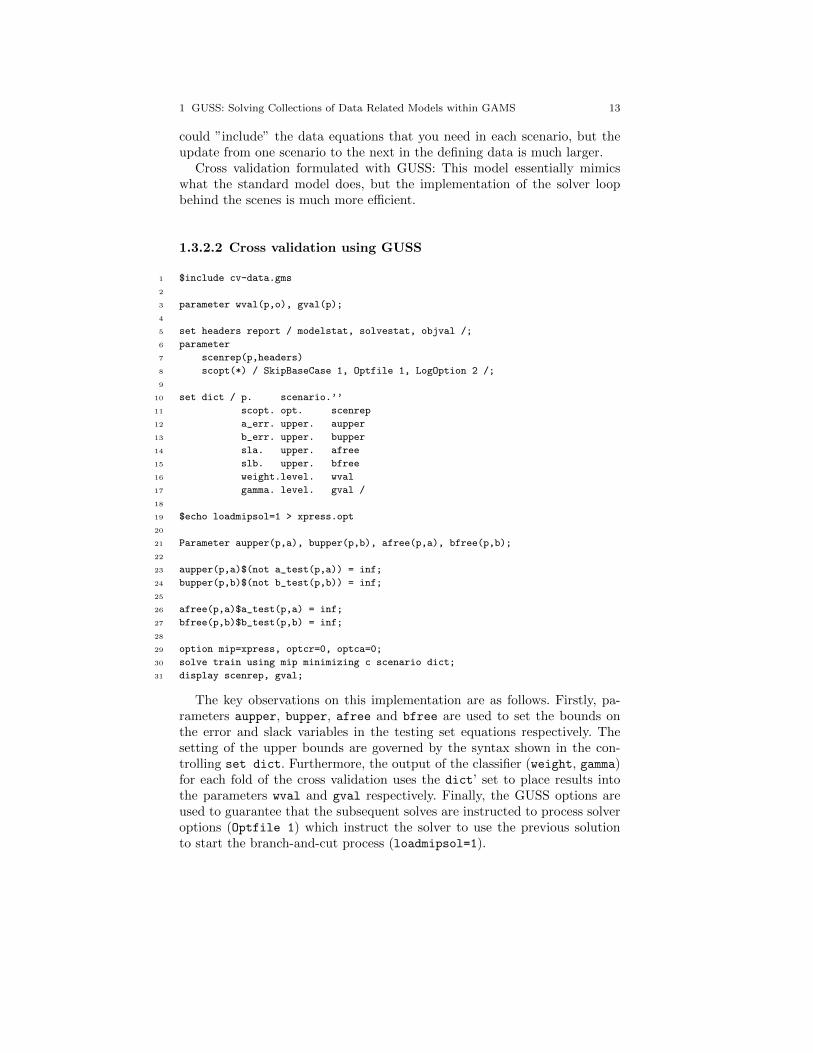
could ”include” the data equations that you need in each scenario, but theupdate from one scenario to the next in the defining data is much larger.
Cross validation formulated with GUSS: This model essentially mimicswhat the standard model does, but the implementation of the solver loopbehind the scenes is much more efficient.
1.3.2.2 Cross validation using GUSS
1 $include cv-data.gms
2
3 parameter wval(p,o), gval(p);
4
5 set headers report / modelstat, solvestat, objval /;
6 parameter
7 scenrep(p,headers)
8 scopt(*) / SkipBaseCase 1, Optfile 1, LogOption 2 /;
9
10 set dict / p. scenario.’’
11 scopt. opt. scenrep
12 a_err. upper. aupper
13 b_err. upper. bupper
14 sla. upper. afree
15 slb. upper. bfree
16 weight.level. wval
17 gamma. level. gval /
18
19 $echo loadmipsol=1 > xpress.opt
20
21 Parameter aupper(p,a), bupper(p,b), afree(p,a), bfree(p,b);
22
23 aupper(p,a)$(not a_test(p,a)) = inf;
24 bupper(p,b)$(not b_test(p,b)) = inf;
25
26 afree(p,a)$a_test(p,a) = inf;
27 bfree(p,b)$b_test(p,b) = inf;
28
29 option mip=xpress, optcr=0, optca=0;
30 solve train using mip minimizing c scenario dict;
31 display scenrep, gval;
The key observations on this implementation are as follows. Firstly, pa-rameters aupper, bupper, afree and bfree are used to set the bounds onthe error and slack variables in the testing set equations respectively. Thesetting of the upper bounds are governed by the syntax shown in the con-trolling set dict. Furthermore, the output of the classifier (weight, gamma)for each fold of the cross validation uses the dict’ set to place results intothe parameters wval and gval respectively. Finally, the GUSS options areused to guarantee that the subsequent solves are instructed to process solveroptions (Optfile 1) which instruct the solver to use the previous solutionto start the branch-and-cut process (loadmipsol=1).
14 Michael R. Bussieck, Michael C. Ferris, and Timo Lohmann
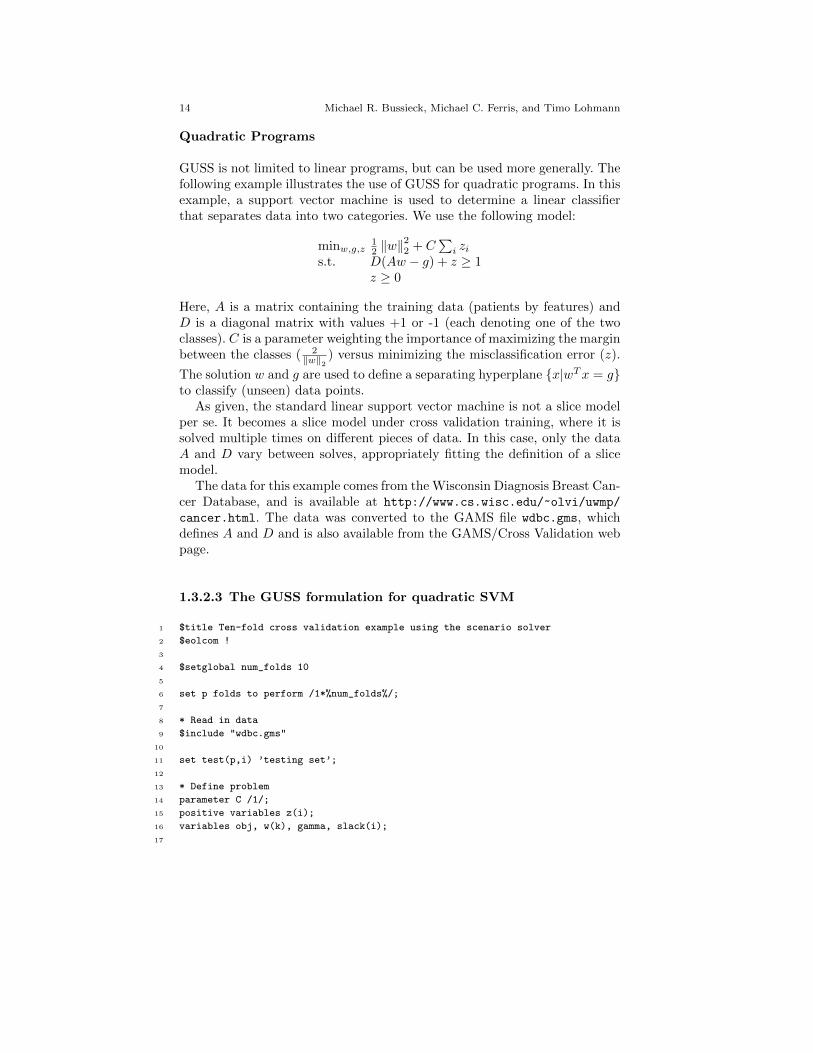
Quadratic Programs
GUSS is not limited to linear programs, but can be used more generally. Thefollowing example illustrates the use of GUSS for quadratic programs. In thisexample, a support vector machine is used to determine a linear classifierthat separates data into two categories. We use the following model:
minw,g,z12 ‖w‖
22 + C
∑i zi
s.t. D(Aw − g) + z ≥ 1z ≥ 0
Here, A is a matrix containing the training data (patients by features) andD is a diagonal matrix with values +1 or -1 (each denoting one of the twoclasses). C is a parameter weighting the importance of maximizing the marginbetween the classes ( 2
‖w‖2) versus minimizing the misclassification error (z).
The solution w and g are used to define a separating hyperplane {x|wTx = g}to classify (unseen) data points.
As given, the standard linear support vector machine is not a slice modelper se. It becomes a slice model under cross validation training, where it issolved multiple times on different pieces of data. In this case, only the dataA and D vary between solves, appropriately fitting the definition of a slicemodel.
The data for this example comes from the Wisconsin Diagnosis Breast Can-cer Database, and is available at http://www.cs.wisc.edu/~olvi/uwmp/
cancer.html. The data was converted to the GAMS file wdbc.gms, whichdefines A and D and is also available from the GAMS/Cross Validation webpage.
1.3.2.3 The GUSS formulation for quadratic SVM
1 $title Ten-fold cross validation example using the scenario solver
2 $eolcom !
3
4 $setglobal num_folds 10
5
6 set p folds to perform /1*%num_folds%/;
7
8 * Read in data
9 $include "wdbc.gms"
10
11 set test(p,i) ’testing set’;
12
13 * Define problem
14 parameter C /1/;
15 positive variables z(i);
16 variables obj, w(k), gamma, slack(i);
17
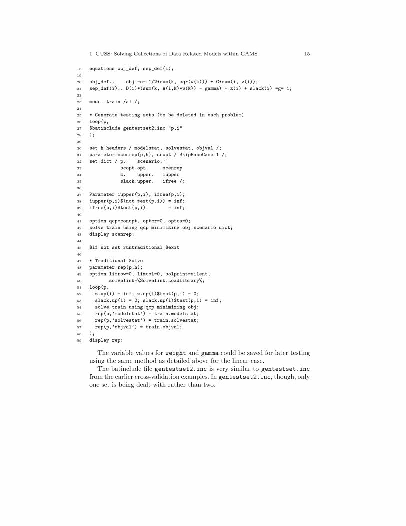
1 GUSS: Solving Collections of Data Related Models within GAMS 15
18 equations obj_def, sep_def(i);
19
20 obj_def.. obj =e= 1/2*sum(k, sqr(w(k))) + C*sum(i, z(i));
21 sep_def(i).. D(i)*(sum(k, A(i,k)*w(k)) - gamma) + z(i) + slack(i) =g= 1;
22
23 model train /all/;
24
25 * Generate testing sets (to be deleted in each problem)
26 loop(p,
27 $batinclude gentestset2.inc "p,i"
28 );
29
30 set h headers / modelstat, solvestat, objval /;
31 parameter scenrep(p,h), scopt / SkipBaseCase 1 /;
32 set dict / p. scenario.’’
33 scopt.opt. scenrep
34 z. upper. iupper
35 slack.upper. ifree /;
36
37 Parameter iupper(p,i), ifree(p,i);
38 iupper(p,i)$(not test(p,i)) = inf;
39 ifree(p,i)$test(p,i) = inf;
40
41 option qcp=conopt, optcr=0, optca=0;
42 solve train using qcp minimizing obj scenario dict;
43 display scenrep;
44
45 $if not set runtraditional $exit
46
47 * Traditional Solve
48 parameter rep(p,h);
49 option limrow=0, limcol=0, solprint=silent,
50 solvelink=%Solvelink.LoadLibrary%;
51 loop(p,
52 z.up(i) = inf; z.up(i)$test(p,i) = 0;
53 slack.up(i) = 0; slack.up(i)$test(p,i) = inf;
54 solve train using qcp minimizing obj;
55 rep(p,’modelstat’) = train.modelstat;
56 rep(p,’solvestat’) = train.solvestat;
57 rep(p,’objval’) = train.objval;
58 );
59 display rep;
The variable values for weight and gamma could be saved for later testingusing the same method as detailed above for the linear case.
The batinclude file gentestset2.inc is very similar to gentestset.inc
from the earlier cross-validation examples. In gentestset2.inc, though, onlyone set is being dealt with rather than two.
16 Michael R. Bussieck, Michael C. Ferris, and Timo Lohmann
1.3.3 SDDP
In the last two sections we did not quantify the performance improvementsachieved by GUSS. In this section we explore the use of GUSS in a decom-position algorithm applied to a large scale model. We discuss in detail therunning times of a traditional GAMS implementation and a GUSS version ofthe implementation. We also compare the running time of an implementationof the algorithm using the ILOG Concert Technology interface to the Cplexsolver.
The Stochastic Dual Dynamic Programming (SDDP) algorithm [19, 20, 25]for solving multi-stochastic linear programs uses, similar to the well knownBenders decomposition [4], the concept of a future cost function (FCF). Thealgorithm works with an underestimating approximation of this FCF by itera-tively adding supporting hyperplanes (Benders cuts) and therefore improvingthe approximation. Let us consider the following multi-stage stochastic linearprogram [5]
min c1x1 + E[min c2(ξ2)x2(ξ2) + · · ·+ E[min cH(ξH)xH(ξH)] · · · ]s.t. W1x1 = h1
T1(ξ2)x1 +W2(ξ2)x2(ξ2) = h2(ξ2)...
TH−1(ξH)xH−1(ξH−1) +WH(ξH)xH(ξH) = hH(ξH)x1 ≥ 0, xt(ξt) ≥ 0, t = 2, ...,H,
where ξt are random variables. The SDDP algorithm requires a Markovianstructure of the coefficient matrix, meaning that a stage only depends onthe previous stage. Furthermore the random variables must be stage-wiseindependent and must follow a discrete distribution. This means ξt can bedescribed as ξt = (ξ1t, ..., ξIt) for a discrete distribution of I realizations withrespective probability pi.The SDDP algorithm decomposes the stochastic linear problem into H sub-problems of the form
min ctxt + αt+1
s.t. Wtxt ≥ ht − Tt−1x∗t−1,αt+1 + πjt+1Ttxt ≥ δ
jt , j = 1, ..., J,
xt ≥ 0,
(SUB(t, ξit, x∗t−1))
where αt+1 is represented by free scalar variables. For reason of conveniencewe omit the random variables in the description. In order to be able to solvea subproblem the previous stage decision variable x∗t−1 must be fixed andtherefore goes to the right hand side. The set j = 1, ..., J denotes the addedhyperplanes to the subproblem, serving as an approximation of the FCF.Throughout the algorithm these kind of subproblems, with different param-eters and variable fixings, are the only problems solved. In order to avoid
1 GUSS: Solving Collections of Data Related Models within GAMS 17
generating and solving them one at a time GUSS allows solving them in cer-tain batches, generating the submodel once for each batch. The details of thisprocess will be shown later in this section.
1.3.3.1 Building of cuts
Each iteration of the SDDP algorithm consists of two phases: a backwardrecursion and a forward simulation. In the backward recursion supportinghyperplanes of the form
αt+1 + πjt+1Ttxt ≥ δjt , (CUTjt )
are added to the subproblems in order to improve the approximate FCF.Suppose we are in iteration j and stage t + 1 of the backward recursion ofthe algorithm and have solved the subproblem SUB(t+ 1, ξi,t+1, x
∗t−1) for all
i = 1, ..., I and dual multipliers πi,t+1 on all constraints with variables of stage
t are stored. In particular this means we may have dual multipliers λji,k,t+1
belonging to cuts that have been added in earlier iterations. We are nowmoving to the previous stage t and want to build CUTjt . For the coefficient
of the cut the sum πjt+1 =∑Ii=1 piπi,t+1 is calculated. Calculating λjk,t+1 is
done in the same way. The cut right hand side δjt is then calculated as follows
δjt =
{∑Ii=1 piπ
ji,t+1hi,t+1, t = H − 1∑I
i=1 piπji,t+1hi,t+1 +
∑jk=1 λ
jk,t+1δ
kt+1, t = 1, ...,H − 2.
A lower bound is computed by solving the first-stage subproblem with cuts.In the forward simulation the approximate FCF is used to construct a fea-sible solution of the problem, resulting in an upper bound to the optimalsolution value. While going forward we sample one realization out of the set{ξ1t, ..., ξIt} and solve the respective subproblem. Note that the only cutsdescribed in this section are optimality cuts. Usually a second type of cut,feasibility cuts, are used for a Benders decomposition. By adding slack vari-ables we made sure that these are not needed for our model.
1.3.3.2 Algorithm in pseudo-code
In the actual algorithm both the backward and forward part is passed throughwith multiple solutions in one iteration. These solutions are called trial solu-tions and they are important for several reasons. In the backward recursionthis leads to one additional cut per trial solution, which results in a betterapproximation of the FCF. In the forward simulation the trial solutions help
18 Michael R. Bussieck, Michael C. Ferris, and Timo Lohmann
to get a more reasonable estimate of the upper bound. The algorithm inpseudo-code reads as follows
1: while convergence is not reached do2: for t = H, ..., 2 (Backward recursion) do3: for each trial solution x∗t−1 do4: for each realization ξit of the random variable do5: Solve SUB(t, ξit, x
∗t−1) and calculate dual multipliers of the
constraints.6: end for7: end for
8: Use dual multipliers to construct the cuts CUTjt−1 and add them toSUB(t− 1, ξi,t−1, x
∗t−2).
9: end for10: for t = 1, ...,H (Forward simulation) do11: for each trial solution x∗t−1 do12: Solve SUB(t, ξit, x
∗t−1) for a sampled realization ξit and store
the solution as x∗t . Fix x∗t for SUB(t+ 1, ξi,t+1, x∗t ).
13: if t = 1 then14: store the objective as LOWER BOUND15: end if16: end for17: end for18: Calculate the UPPER BOUND using the stored solutions.19: Check for convergence.20: end while
GUSS allows us to rewrite the various SOLVE statements in GAMS in theinner loop of the backward recursion (lines 3-7) into one SOLVE statement. Inspecific, we write all possible combinations of trial solutions and realizationsinto the scenario dict. This results in one SOLVE statement per stage andeach of these SOLVE statements will solve (#trials × #realizations) manymodels without regenerating them. In the forward simulation we can rewritethe SOLVE statements in GAMS in the inner loop (lines 11-12). This againresults in one SOLVE statement per stage instead of having #trials manySOLVE statements.
1.3.3.3 Results
The SDDP algorithm has been implemented for a stochastic linear programmotivated by Vattenfall Energy Trading, a branch of the Swedish power com-pany Vattenfall. The objective of the model is to minimize the power gener-ation costs and ultimately to forecast power prices of the market. Power canbe generated by an aggregated hydro power plant, a coal plant, or a nuclear
1 GUSS: Solving Collections of Data Related Models within GAMS 19
plant. Using hydro power has no costs, but there is a limited amount of wa-ter in the reservoir and limited inflows of water into the reservoir over time.In each time period, water can be either used for power generation, saved,or spilled. The model has a granularity of hours and is set up for one year,which results in 8736 time periods. Stochastic information is revealed everyweek, resulting in 52 stages. A one-stage sub-model therefore consists of 168hours. In order to compare different implementations of the algorithm, werecorded the time for the first 20 iterations. We used five trial solutions anda discrete distribution made of twelve realizations. During the course of the20 iterations 66,320 linear programs have been solved. To make runs compa-rable we worked with a random but fixed sampling (line 12 of the algorithm)in all implementations. All experiments were carried out on a PC with anIntel i7-680 chip running Windows 7 (64bit) with GAMS version 23.7.0 andCplex 12.2.0.2. We implemented three versions of the algorithm:
Traditional: This is a GAMS model implementing the SDDP algorithmwith traditional GAMS programming flow control structures like loop.This traditional version has been tested with three different ways of callingthe LP solver which is parameterized by the GAMS option solvelink.ChainScript, which is the default in GAMS, produces for each SOLVE
statement some scratch files on disk containing the model instance, italso dumps the entire GAMS database into a scratch file and stops theGAMS runtime system leaving all computer resources to the solver job.After the solver job terminates, the GAMS runtime system reinitializesitself from the GAMS database scratch file and continues with executionof the GAMS program. CallModule also creates creates files for a modelinstance but the GAMS runtime system stays in memory while the solverjob runs. LoadLibrary communicates the model instance through memoryand initiates the solver through a shared library. This implementation isavailable at http://www.gams.com/modlib/adddocs/sddp_trad.gms.
GUSS: This implementation replaces parts of the traditional loop con-structs in the traditional GAMS model by scenario based SOLVE state-ments using GUSS as discussed above. This model is part of the GAMSModel Library (http://www.gams.com/modlib/libhtml/sddp.htm)
Concert: This implementation is based on ILOG Concert Technology, aprogramming interface to generate and solve linear, quadratic and con-straint programming based models with solvers available from the IBMCplex Optimization Studio. This particular C++ implementation usedConcert to generate linear programming model and solve them withCplex. The C++ program is available at http://www.gams.com/modlib/adddocs/sddp.cpp. The model data (and the random data for sampling)comes from GAMS through the Gams Data eXchange (GDX).
All three implementations build on the same core LP technology, the Cplexdual simplex engine. The accumulated time spent in the core Cplex optimizer(CPXlpopt) for the 66,320 linear programs amounts to approximately 110 sec-
20 Michael R. Bussieck, Michael C. Ferris, and Timo Lohmann
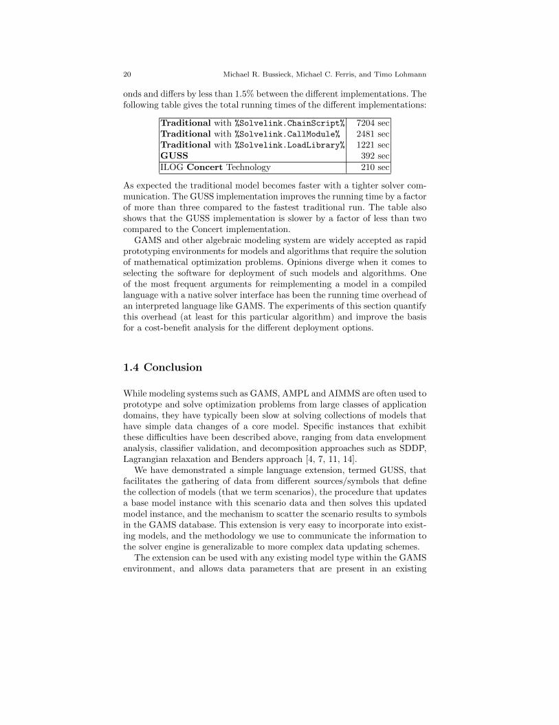
onds and differs by less than 1.5% between the different implementations. Thefollowing table gives the total running times of the different implementations:
Traditional with %Solvelink.ChainScript% 7204 secTraditional with %Solvelink.CallModule% 2481 secTraditional with %Solvelink.LoadLibrary% 1221 secGUSS 392 sec
ILOG Concert Technology 210 sec
As expected the traditional model becomes faster with a tighter solver com-munication. The GUSS implementation improves the running time by a factorof more than three compared to the fastest traditional run. The table alsoshows that the GUSS implementation is slower by a factor of less than twocompared to the Concert implementation.
GAMS and other algebraic modeling system are widely accepted as rapidprototyping environments for models and algorithms that require the solutionof mathematical optimization problems. Opinions diverge when it comes toselecting the software for deployment of such models and algorithms. Oneof the most frequent arguments for reimplementing a model in a compiledlanguage with a native solver interface has been the running time overhead ofan interpreted language like GAMS. The experiments of this section quantifythis overhead (at least for this particular algorithm) and improve the basisfor a cost-benefit analysis for the different deployment options.
1.4 Conclusion
While modeling systems such as GAMS, AMPL and AIMMS are often used toprototype and solve optimization problems from large classes of applicationdomains, they have typically been slow at solving collections of models thathave simple data changes of a core model. Specific instances that exhibitthese difficulties have been described above, ranging from data envelopmentanalysis, classifier validation, and decomposition approaches such as SDDP,Lagrangian relaxation and Benders approach [4, 7, 11, 14].
We have demonstrated a simple language extension, termed GUSS, thatfacilitates the gathering of data from different sources/symbols that definethe collection of models (that we term scenarios), the procedure that updatesa base model instance with this scenario data and then solves this updatedmodel instance, and the mechanism to scatter the scenario results to symbolsin the GAMS database. This extension is very easy to incorporate into exist-ing models, and the methodology we use to communicate the information tothe solver engine is generalizable to more complex data updating schemes.
The extension can be used with any existing model type within the GAMSenvironment, and allows data parameters that are present in an existing
1 GUSS: Solving Collections of Data Related Models within GAMS 21
model to be identified (and updated) using a scenario index. We have demon-strated its utility on a number of example applications and have shown dis-tinct improvements in speed of processing these collections of models. Webelieve that models updated to use GUSS will be competitive with nativeimplementations of decomposition algorithms, but will have the distinct ad-vantage that they will be much easier to code, available to a modeler to tailorto a specific idea, and enable new suites of problems to be solved directlywithin the modeling system.
References
1. Banker, R.D., Charnes, A., Cooper, W.W.: Some models for estimating technical andscale inefficiencies in Data Envelopment Analysis. Management Science 30(9), 1078–
1092 (1984)
2. Banker, R.D., Morey, R.C.: Efficiency analysis for exogenously fixed inputs and out-puts. Operations Research 34(4), 513–521 (1986)
3. Banker, R.D., Morey, R.C.: The use of categorical variables in Data Envelopment
Analysis. Management Science 32(12), 1613–1627 (1986)4. Benders, J.F.: Partitioning procedures for solving mixed-variables programming prob-
lems. Numerische Mathematik 4(1), 238–252 (1962)5. Birge, J.R., Louveaux, F.: Introduction to Stochastic Programming. Springer Verlag
(1997)
6. Bussieck, M.R., Ferris, M.C., Meeraus, A.: Grid enabled optimization with GAMS.INFORMS Journal on Computing 21(3), 349–362 (2009)
7. Carøe, C.C., Schultz, R.: Dual decomposition in stochastic integer programming. Op-
erations Research Letters 24, 37–45 (1999)8. Charnes, A., Cooper, W., Lewin, A.Y., Seiford, L.M.: Data Envelopment Analysis:
Theory, Methodology and Applications. Kluwer Academic Publishers, Boston, MA
(1994)9. Charnes, A., Cooper, W.W., Rhodes, E.: Measuring the efficiency of decision making
units. European Journal of Operational Research 2, 429–444 (1978)
10. Cooper, W.W., Seiford, L.M., Tone, K.: Data Envelopment Analysis: A Comprehen-sive Text with Models, Applications, References and DEA-Solver Software. Kluwer
Academic Publishers, Boston, MA (2000)
11. Dantzig, G.B., Wolfe, P.: Decomposition principle for linear programs. OperationsResearch 8, 101–111 (1960)
12. Efron, B., Tibshirani, R.: Improvements on cross-validation: The .632 + bootstrapmethod. Journal of the American Statistical Association 92, 548–560 (1997)
13. Farrell, M.J.: The measurement of productive efficiency. Journal of the Royal Statis-tical Society, Series A (General) 120(3), 253–290 (1957)
14. Ferris, M.C., Maravelias, C.T., Sundaramoorthy, A.: Simultaneous batching andscheduling using dynamic decomposition on a grid. INFORMS Journal on Computing
21(3), 398–410 (2009)15. Ferris, M.C., Voelker, M.M.: Slice models in general purpose modeling systems: An
application to DEA. Optimization Methods and Software 17, 1009–1032 (2002)16. Geisser, S.: Predictive Inference. Chapman and Hall, New York (1993)17. Kohavi, R.: A study of cross-validation and bootstrap for accuracy estimation and
model selection. In: Proceedings of the Fourteenth International Joint Conference on
Artificial Intelligence 2, p. 11371143. Morgan Kaufmann, San Mateo (1995)
22 Michael R. Bussieck, Michael C. Ferris, and Timo Lohmann
18. Olesen, O.B., Petersen, N.C.: A presentation of GAMS for DEA. Computers and
Operations Research 23(4), 323–339 (1996)19. Pereira, M.V.F., Pinto, L.M.V.G.: Stochastic optimization of a multireservoir hydro-
electric system: A decomposition approach. Water Resources Research 21(6), 779–792
(1985)20. Pereira, M.V.F., Pinto, L.M.V.G.: Multi-stage stochastic optimization applied to en-
ergy planning. Mathematical Programming 52, 359–375 (1991)
21. Picard, R., Cook, D.: Cross-validation of regression models. Journal of the AmericanStatistical Association 79, 575–583 (1984)
22. Seiford, L.M., Zhu, J.: Sensitivity analysis of DEA models for simultaneous changesin all the data. Journal of the Operational Research Society 49, 1060–1071 (1998)
23. Simar, L., Wilson, P.W.: Sensitivity analysis of efficiency scores: How to bootstrap in
nonparametric frontier models. Management Science 44(1), 49–61 (1998)24. Thanassoulis, E., Boussofiane, A., Dyson, R.G.: Exploring output quality targets in
the provision of perinatal care in England using DEA. European Journal of Operations
Research 60, 588–608 (1995)25. Velasquez, J., Restrepo, P., Campo, R.: Dual dynamic programming: A note on im-
plementation. Water Resources Research 35(7) (1999)