Embed Size (px)
Citation preview

1
Chapter 1: General Introduction
1.1. Nature of Electromagnetic Radiation
The electric and magnetic fields (E and B) generated by an electric dipole (i.e. by a pair
of positive and negative charges) are simply the sum of the fields from the individual charges. If
the orientation of the dipole oscillates with time, the fields in the vicinity will also oscillate at the
same frequency. The oscillating components of E and B at a given position are perpendicular to
each other, and at large distances from the dipole, they also are perpendicular to the position
vector (r) relative to the center of the dipole. They fall off in magnitude with 1/r, and with the
sine of the angle (θ) between r and the dipole axis. Such a coupled set of oscillating electric and
magnetic fields together constitute an electromagnetic (EM) radiation field.
A spreading radiation field like that mentioned above can be collimated by a lens or
mirror to generate a plane wave that propagates in a single direction with constant irradiance
(measure of the strength of EM radiation and expressed in terms of the amount of energy
flowing across a specified plane per unit area per unit time). The electric and magnetic fields in
such a wave oscillate sinusoidally along the propagation axis as illustrated in figure 1.1, but are
independent of position normal to this axis. Polarizing devices can be used to restrict the
orientation of the electric and magnetic fields to a particular axis in the plane. The plane wave
illustrated in figure 1.1 is said to be linearly polarized because the electric field vector is always
parallel to a fixed axis. Because E is confined to the plane normal to the axis of propagation, the
wave also can be described as plane-polarized. An unpolarized light beam propagating in the y-
direction consists of electric and magnetic fields oscillating in the xz plane at all angles with
respect to the z-axis.
The properties of EM fields are described empirically by four coupled equations that
were set forth by J.C. Maxwell in 1865 [1]. These very general equations apply to both static and
oscillating fields, and they encapsulate the salient features of EM radiation. In words, they state
that: (i) Both E and B are always perpendicular to the direction of propagation of the radiation
(i.e., the waves are transverse); (ii) E and B are perpendicular to each other; (iii) E and B oscillate
in phase; and, (iv) If we look in the direction of propagation, a rotation from the direction of E to
the direction of B is clockwise. Instead of putting too much stress on the Maxwell’s equations
themselves; we can focus on a solution to these equations for a particular situation such as the

2
plane wave of monochromatic, polarized light illustrated in figure 1.1. In molecular
spectroscopy, one is interested mainly in the time-dependent oscillations of the electrical and
magnetic fields in small, fixed regions of space. Because molecular dimensions typically are
much smaller than the wavelength of visible light, the amplitude of the electrical field at a
particular time will be nearly the same everywhere in the molecule. One can also take the
average of the field over many cycles of the oscillation initially and assume that it does not
depend on coherent superposition of light beams with fixed phase relationships. With these
restrictions, the dependence of E on position and the phase shift can be neglected, and written
as (taking as the frequency of oscillation)
푬(푡) = 2푬ퟎ cos(2휋푡) = 푬ퟎ(푒 + 푒 ) (1.1)
Figure 1.1 Electric (bold curve) and magnetic (light curve) field components as a function of position at a given time in a linearly polarized plane wave propagating in the direction of y-axis.
1.2. Interaction of Electrons with Oscillating Electric Field
In this section, we will see how an oscillating electric field of linearly polarized light (with
frequency ), interacts with the molecule to cause electronic absorption. The oscillating electric
field adds a time-dependent term to the stationary state Hamiltonian operator (Ĥ) for the

3
electron. To an approximation that often proves acceptable, we can write the perturbation (ĥ)
as the dot product of E with the dipole operator, :
ĥ(푡) = −푬(푡). (1.2)
The dipole moment operator, , for an electron can simply be written as:
= 푒풓 (1.3) where, e (= -1.602 × 10⁻¹⁹ C) is the electronic charge, r is the position vector and r is the position
of the electron. Putting E(t) in equation (1.2) from equation (1.1), one can write
ĥ(푡) = −푒푬(푡). 푟 = −푒|푬ퟎ|(푒 + 푒 )|푟| cos휃 (1.4)
where, r is the position of the electron and is the angle between E0 and r.
In the ground state, the wavefunction of the molecule (electron) can be described by a.
However, in presence of an oscillating radiation field, this and the other solutions to the
Schrödinger equation for the unperturbed system become unsatisfactory; they no longer
represent the stationary states. Normally, the wavefunction of the electron in the presence of
the field can be expressed by a linear combination of the original wavefunctions; CaΨa + CbΨb+...,
where the coefficients Ck are functions of time. As long as the system is still in Ψa, Ca = 1 and all
the other coefficients are zero; but if the perturbation is sufficiently strong Ca will decrease with
time, while Cb or other coefficients increases. The expected rate of growth of Cb can be given by:
휕퐶푏휕푥 = 푒 푒 + 푒 푬ퟎ. ⟨휓 |흁|휓 ⟩ (1.5)
= 푒 + {푒 }푬ퟎ. ⟨휓 |흁|휓 ⟩ (1.6)
where, Ea and Eb are the energies of states a and b (represented by a and b), respectively.
The probability that the electron has made a transition from Ψa to Ψb by time τ is
obtained by integrating the above equation from time t = 0 to τ and then evaluating |Cb(τ)|2.
The result gives:

4
퐶 (휏) = × {푒 − 1} + × {푒 − 1} × 푬ퟎ. ⟨휓 |휇|휓 ⟩
(1.7)
It is to be noted that the two fractions in the first term differ only in the sign of the term
h. Let us assume the situation where Eb > Ea, which means that Ψb lies above Ψa in energy. The
denominator in the second fraction of the first term then becomes zero when Eb − Ea = h. The
numerator of this term is a complex number, but its magnitude also goes to zero under this
condition, and the ratio of the numerator to the denominator becomes 2πiτ/h. On the other
hand, if, Eb < Ea (i.e., if Ψb lies below Ψa), then the ratio of the numerator to the denominator in
the first term in the large parentheses becomes 2πiτ/h when Ea − Eb = hν. If |Eb − Ea| is very
different from h, both terms will be very small. So something special evidently happens if h is
close to the energy difference between the two states. Basically, the second term in the large
bracket in equation (1.7) accounts for absorption of light when Eb − Ea = hν, and that the first
term accounts for induced or stimulated emission of light when Ea−Eb = hν. Stimulated emission,
a downward electronic transition in which light is given off, is just the reverse of absorption.
1.3. Regions of Electromagnetic Spectrum
The regions of the electromagnetic spectrum that will be the most pertinent for the
discussion of molecular spectroscopy involve wavelengths between 10−9 and 10−2 cm. Visible
light fills only the small part of this range between 3×10⁻⁵ and 8 × 10⁻⁵ cm (figure 1.2).
Transitions of bonding electrons occur mainly in this region and the neighboring UV region;
vibrational transitions occur in the infra-red (IR). Rotational transitions are measurable in the
far-IR (microwave) region in small molecules, but in macromolecules these transitions are too
congested to resolve. Radiation in the X-ray region can cause transitions in which 1s or other
core electrons are excited to atomic 3d or 4f shells or are dislodged completely from a molecule.
These transitions can report on the oxidation and coordination states of metal atoms in metallo-
proteins.
The inherent sensitivity of absorption measurements in different regions of the
electromagnetic spectrum decreases with increasing wavelength because, in the idealized case
of a molecule that absorbs and emits radiation at a single frequency, it depends on the
difference between the populations of molecules in the ground and excited states. If the two

5
populations are the same, radiation at the resonance frequency will cause upward and
downward transitions at the same rate, giving a net absorbance of zero [2].
Figure 1.2 Regions of electromagnetic spectrum shown in logarithmic wavelength, wavenumber, frequency and energy scales. The upper panel is the enlarged ultraviolet (UV), visible and infra-red (IR) region presented in a linear scale.
1.4. Electronic Absorption
1.4.1. Quantification of light absorption: The Beer-Lambert law
A beam of light passing through a solution of absorbing molecules transfers energy to
the molecules as it proceeds, and thus decreases progressively in intensity. The decrease in the
intensity, or irradiance (I), over the course of a small volume element is proportional to the

6
irradiance of the light entering the element, the concentration of absorbers (c), and the length
of the path through the element (dx):
푑퐼푑푥 = −휀′퐼푐 (1.8)
The proportionality constant (’) depends on the wavelength of the light and on the
absorber’s structure, orientation and environment. Integrating equation (1.8) shows that if light
with irradiance I0 is incident on a cell of thickness l, the irradiance of the transmitted light will
be:
퐼 = 퐼 × 푒 = 퐼 × 10 = 퐼 × 10 (1.9)
where, A is the absorbance or optical density of the sample (A = εCl) and ε is called the
molar extinction coefficient or molar absorption coefficient (ε = ε’/ ln 10 = ε’/2.303). The
absorbance is a dimensionless quantity, so if c is given in units of molarity (1M = 1 mol dm−3) and
l in cm, ε must have dimensions of M−1 cm−1. Equations (1.8) and (1.9) are statements of Beer’s
law, or more accurately, the Beer–Lambert law [3].
1.4.2. Techniques of measuring absorbance
A spectrophotometer for measuring absorption spectra typically includes a continuous
light source, a monochromator for dispersing the white light and selecting a narrow band of
wavelengths, and a chopper for separating the light into two beams (figure 1.3). One beam
passes through the specimen of interest; the other through a reference (blank) cuvette. The
intensities of the two beams are measured with a photomultiplier or other detector, and are
used to calculate the absorbance of the sample as a function of wavelength [ΔA = log10(I0/Is) −
log10(I0/Ir) = log10(Ir/Is), where I0, Is, and Ir are the incident light intensity and the intensities of the
light transmitted through the specimen and reference, respectively]. The measurement of the
reference signal allows the instrument to discount the absorbance due to the solvent and the
walls of the cuvette. Judicious choice of the reference also can minimize errors resulting from
the loss of light by scattering from turbid samples.

7
Figure 1.3 Different elements of a modern spectrophotometer. PD indicates a photo-detector in the form of photomultiplier or photodiode.
The conventional spectrophotometer sketched in figure 1.3 has several limitations. First,
the light reaching the detector at any given time covers only a narrow band of wavelengths.
Because a grating, prism, or mirror in the monochromator must be rotated to move this window
across the spectral region of interest, acquisition of an absorption spectrum typically takes
several minutes, during which time the sample may change. In addition, narrowing the entrance
and exit slits of the monochromator to improve the spectral resolution decreases the amount of
light reaching the photomultiplier, which makes the signal noisier. Although the signal-to- noise
ratio can be improved by averaging the signal over longer periods of time, this further slows
acquisition of the spectrum. These limitations are surmounted to some extent in instruments
that use photodiode arrays to detect light at many different wavelengths simultaneously.
1.4.3. Effect of surrounding on electronic transition energy
Interactions with the surroundings can shift the energy of an absorption band to either
higher or lower energies, depending on the nature of the chromophore and the solvent. For
example, considering an n→π∗ transition, in which an electron is excited from a nonbonding
orbital of an oxygen atom to an antibonding molecular orbital distributed between oxygen and
carbon atoms. In the ground state, electrons in the nonbonding orbital can be stabilized by
hydrogen-bonding or dielectric effects of the solvent. In the excited state, these favorable
interactions are disrupted. Although solvent molecules will tend to reorient themselves in
response to the new distribution of electrons in the chromophore, this reorientation is too slow
to occur during the excitation itself. An n→π∗ transition therefore shifts to higher energy in
more polar or hydrogen-bonding solvents relative to less polar solvents. A shift of an absorption

8
band in this direction is called a “blue-shift.” On the other hand, the energies of π→π∗
transitions are less sensitive to the polarity of the solvent but still depend on the solvent’s high-
frequency polarizability, which increases quadratically with the refractive index. Increasing the
refractive index usually decreases the transition energy of a π→π∗ transition, causing a “red-
shift” of the absorption band.
1.4.4. Relaxation of electronically excited molecules
The mechanisms by which electronically excited molecules come to ground state are
given by the Jablonski diagram as shown in figure 1.4 The absorption of a photon takes the
molecule from ground singlet state (So) to either first or second excited singlet states
(represented by S1 or S2, respectively). From this Franck-Condon (FC) excited state, the molecule
relaxes to the lowest vibronic level of the S1 state through internal conversion (IC). Further
relaxation from this state to S0 can occur via three mechanisms. First, by radiative emission of a
photon and the process is called as fluorescence. The other two non-radiative channels involve
either direct relaxation to S0 state (internal conversion) or passage to the triplet state (T1) by
intersystem crossing (ISC). The radiative transition from T1 to So state is quantum mechanically
forbidden and hence is a very slow process relative to fluorescence and is called
phosphorescence emission. The fluorescence photons have the information about energy, time,
polarization and intensity at a given wavelength. Each of the above parameters of the
fluorescence photon gives information about the local environment surrounding the
fluorophore under investigation. So, fluorescence intensity, spectrum, polarization and their
dependence are important parameters that one can use for the characterization [4].
The maximum of phosphorescence spectrum is generally shifted to longer wavelength
relative to the fluorescence. Also, the S1 state can be deactivated by a quenching mechanism, in
which a quencher Q quenches the excited state of the fluorophore (S1) through an excited state
reaction. Reverse intersystem crossing from T1 to S1 can occur when the energy between S1 and
T1 is small and when the lifetime of T1 is long enough. This results in emission with the same
spectral distribution as normal fluorescence but with a much longer decay time constant
because the molecules stay in the triplet state before emitting from S1. This fluorescence
emission is thermally activated; consequently, its efficiency increases with temperature and is
called delayed fluorescence of E-type. Again, in concentrated solutions, a collision between two
molecules in the T1 state can provide enough energy to allow one of them to return to the S1

9
state. Such triplet-triplet annihilation thus leads to a delayed fluorescence emission, and termed
as delayed fluorescence of P-type.
Figure 1.4 Schematic representation of Jablonski diagram.
In table 1.1, all possible photochemical pathways those can occur during a photo-
excitation and de-excitation process, are shown. If the excited state decayed solely by
fluorescence, its population would decrease exponentially with time and the time constant of
the decay would be τr (reciprocal of the radiative rate constant, r) . However, other decay
mechanisms compete with fluorescence, decreasing the radiative lifetime of the excited state.
The alternatives include formation of triplet states (intersystem crossing) with rate constant
isc, nonradiative decay (internal conversion) to the ground state (ic). Radiative decay from the
triplet state (phosphorescence with corresponding rate constant, p) can also be another
alternative relaxation pathway. Further, several excited state processes like transfer of energy
to other molecules (resonance energy transfer, krt), electron and proton transfer (et and pt,
respectively) can also contribute hugely in the de-excitation mechanism.

10
Table 1.1 Different photophysical processes, associated transition and other relevant parameters
Process Transition Rate constant Timescale (s) (a) Absorption (Excitation) 푆 → 푆 표푟 푆 Instantaneous 10-15
(b) Internal Conversion 푆 → 푆 ic 10-1410-10
(c) Vibrational Relaxation 푆 → 푆 vr 10-1210-10 (d) Fluorescence 푆 → 푆 f 10-910-7 (e) Intersystem Crossing 푆 → 푇 isc 10-1010-8 (f) Non-radiative Relaxation,
Quenching 푆 → 푆 nr, q 10-710-5
(g) Phosphorescence 푇 → 푆 p 10-3102 (h)
Non-radiative Relaxation, Quenching
푇 → 푆 nr, q 10-3102
1.5. Molecular Fluorescence
1.5.1. Fluorescence intensity and spectra
The amount of fluorescence photons emitted per unit time and per unit volume is called
the steady state fluorescence intensity (I). The steady state fluorescence intensity per absorbed
photon as a function of the wavelength of the emitted photons represents the fluorescence
spectrum or emission spectrum which reflects the distribution of the probability of the various
transitions from the lowest vibrational level of S1 to the various vibrational levels of S0. The
intensity versus wavelength plot (fluorescence emission spectrum) is characteristic of a
fluorophore and sensitive to its local surrounding environment and consequently used to probe
the structure of the local environment. The fluorescence emission spectrum is generally
independent of excitation wavelength. This is because of the rapid relaxation to the lowest
vibrational level of S1 prior to emission; irrespective of excitation to any higher electronic and
vibrational levels.
1.5.2. The stokes shift
The fluorescence emission spectrum of a molecule in solution usually peaks at a longer
wavelength than the absorption spectrum because nuclear relaxations of the excited molecule
and the solvent transfer some of the excitation energy to the surroundings before the molecule
fluoresces. The red-shift of the fluorescence is called the Stokes shift after George Stokes, a

11
British mathematician and physicist and generally represented in the unit of wavenumber (cm-1)
with the symbol ∆νss. This important parameter provides information on the excited state. As an
example, when the dipole moment of a fluorescent molecule is higher in the S1 state than in S0
state, the magnitude of ∆νss increases with increase in solvent polarity. The Stokes shift reflects
both intramolecular vibrational relaxations of the excited molecule and relaxations of the
surrounding solvent.
Figure 1.5 Potential energy curves for a harmonic oscillator in the ground and excited electronic states. The vibrational reorganization energy () and the bond length displacement () in the ground and excited states are also shown.

12
The contributions from intramolecular vibrations can be related to displacements of the
vibrational potential energy curves between the ground and excited states. Figure 1.5 illustrates
this relationship. Suppose that a particular bond has length bgr at the potential minimum in the
ground state, and length bex in the excited state. The vibrational reorganization energy (Λ) is the
energy required to stretch or compress the bond by (bex− bgr). Classically, this energy is (K/2)(bex
– bgr)2, where K is the vibrational force constant. The quantum-mechanical coupling strength (S)
for a vibrational mode is defined as Δ2/2, where Δ is the dimensionless displacement of the
potential surface in the excited state, 2π(m/h)1/2(bex – bgr), and is the vibrational frequency. It
is well known that in cases where |Δ| > 1, the Franck–Condon factors for absorption peak
occurs at an energy approximately Sh above the 0–0 transition energy. The quantum-
mechanical reorganization energy for a strongly coupled vibrational mode thus is approximately
Sh, or Δ2h/2. If this is the only vibrational mode with a significant coupling strength,
fluorescence emission will peak approximately Sh below the 0–0 transition energy, so the
Stokes shift (habs − hfl in figure 1.5) will be roughly 2Sh, or Δ2h. If multiple vibrational modes
are coupled to the transition, the vibrational Stokes shift is the sum of the individual
contributions: hνabs − hνfl ≈ i |Δi|2hi where Δi and i are the displacement and frequency of
mode i.
A plot analogous to those in figure 1.5 also can be used to describe the dependence of
the energies of the ground and excited states on a generalized solvent coordinate. Neglecting
rotational energies, the overall reorganization energy is the sum of the vibrational and solvent
reorganization energies, and the total Stokes shift is the sum of the vibrational and solvent
Stokes shifts.
1.5.3. The mirror-image rule
The fluorescence emission spectrum of a molecule is approximately a mirror image of
the absorption spectrum, as illustrated in figure 1.6. Several factors contribute to this symmetry.
First, if the Born–Oppenheimer approximation holds, and if the vibrational modes are harmonic
and have the same frequencies in the ground and excited electronic states (all significant
approximations), then the energies of the allowed vibronic transitions in the absorption and
emission spectra will be symmetrically located on opposite sides of the 0–0 transition energy,
hν00. The solid vertical arrows in figure 1.5 illustrate such a pair of upward and downward

13
transitions whose energies are, respectively, h00 + 3h and hν00 − 3h, where is the
vibrational frequency. In general, for fluorescence at frequency = 00 − δ, the corresponding
absorption frequency is ’ = 00 + δ = 200 − . Conversely, absorption at frequency ν’ gives rise
to fluorescence at 200 – ’.
Figure 1.6 Mirror symmetry in the absorption and fluorescence emission spectrum.
Mirror-image symmetry also requires that the Franck–Condon factors be similar for
corresponding transitions in the two directions, and this often is the case. In addition to
requiring matching of the energies and Franck–Condon factors for corresponding upward and
downward transitions, mirror-image symmetry requires the populations of the various
vibrational sublevels from which downward transitions embark in the excited state to be similar
to the populations of the sublevels where corresponding upward transitions originate in the
ground state. This matching will flow from the similarity of the vibrational energies in the
ground and excited states, provided that the vibrational sublevels of the excited state reach
thermal equilibrium rapidly relative to the lifetime of the state. If the excited molecule decays
before it equilibrates, the emission spectrum will depend on the excitation energy and typically
will be shifted to higher energies than the mirror-image law predicts. The mirror-image
relationship can break down for a variety of reasons, including heterogeneity in the absorbing or
emitting molecules, differences between the vibrational frequencies in the ground and excited
states, and failure of the vibrational levels of the excited molecule to reach thermal equilibrium.

14
1.5.4. Fluorescence yield and lifetime
Because the rate constant of different parallel processes (mentioned in section 1.4.4)
add, the actual lifetime of the excited state (the fluorescence lifetime, f) is less than the
radiative lifetime (r):
휏 = < 휏 = (1.10)
where, 휅 = 휅 + 휅 + 휅 + 휅 + ∑휅 (1.11)
The fluorescence yield (φf) is the fraction of the excited molecules that decay by
fluorescence. For a homogeneous sample that emits exclusively from the first excited singlet
state, this is simply the ratio of r to total:
휙 =
= = (1.12)
The fluorescence yield from a homogeneous sample is, therefore, proportional to the
fluorescence lifetime and can provide the same information. However, the situation is little
more complicated in real situations even for the simplest fluorophore and needs proper care
before making a conclusion.
1.5.5. Fluorescence anisotropy The fluorescence emission, emitted from the samples excited with polarized light is also
polarized. This polarization is due the photo-selection of the fluorophores according to their
orientation relative to the direction of the polarized excitation. This photo-selection is
proportional to the square of the cosine of the angle between the absorption dipole of the
fluorophore and the axis of polarization of the excitation light. The orientational anisotropic
distribution of the excited fluorophore population relaxes by rotational diffusion of the
fluorophores and excitation energy transfer to the surrounding acceptor molecules. The
polarized fluorescence emission becomes depolarized by such processes. The fluorescence
anisotropy measurements reveal the average angular displacement of the fluorophore which

15
occurs between absorption and subsequent emission of a photon. The steady state fluorescence
anisotropy (r) is defined by the following equation:
푟 = ∥
∥ (1.13)
where F|| and F represent the fluorescence intensities when the orientation of the emission
polarizer is parallel and perpendicular to the orientation of the excitation polarizer, respectively.
The fluorescence anisotropy (r) is a measure of the average depolarization during the lifetime of
the excited fluorophore under steady state conditions. If a sample contains a mixture of
components with different anisotropies, the observed anisotropy is simply the sum:
푟 = ∑ 휉 푟 (1.14)
where ri is the anisotropy of component i and i is the fraction of the total fluorescence emitted
by this component.
The denominator in the equation (1.13) is proportional to the total fluorescence, FT,
which includes components polarized along all three cartesian axes: FT = Fx + Fy + Fz. If the
excitation is done along z polarization and the fluorescence is measured with polarizers parallel
to the z- and x-axes, then F|| = Fz and F = Fx. Because the emission must be symmetrical in the xy
plane, Fy = Fx. Thus, FT = Fz + 2Fx = F|| + 2F . The total fluorescence also can be obtained by
measuring the fluorescence through a polarizer set at the “magic angle” 54.7◦ from the z-axis, as
shown in figure 1.7. This is equivalent to combining z- and x-polarized measurements with
weighting factors of cos2(54.7◦) and sin2(54.7◦), which have the appropriate ratio of 1:2.
Fluorescence measured through a polarizer at the magic angle with respect to the excitation
polarization is not affected by rotation of the emitting chromophore.
But the time resolved measurements of fluorescence anisotropy using ultrafast
polarized excitation source (laser) give insight into the time dependent depolarization. The time
dependent fluorescence anisotropy or fluorescence anisotropy decay, r(t), is defined as follows.
푟(푡) = ∥( ) ( )
∥( ) ( ) (1.15)

16
Figure 1.7 If a sample is excited with light polarized parallel to the z-axis, the total
fluorescence is proportional to the fluorescence measured at right angles to the excitation through a polarizer at the “magic angle” of 54.7º with respect to z. This measurement weights z and x polarizations in the ratio of 1:2.
where F||(t) and F⊥(t) are the time-dependent fluorescence intensity decays collected with the
polarization of the emission polarizer kept parallel and perpendicular to the polarization of the
excitation source respectively. For a fluorophore in a simple solvent, the fluorescence
depolarization is simply due to rotational motion of the excited fluorophore and the decay
parameters depend on the size and shape of the fluorophore. For spherical fluorophores, the
anisotropy decay is a single exponential with a single rotational correlation time and is shown in
the following equation.
푟(푡) = 푟 exp( − 푡 Θ)⁄ (1.16)
Where, r0 is initial anisotropy (anisotropy at time t = 0 or anisotropy observed in the absence of
any depolarizing processes) and Θ is the rotational correlation time. The initial anisotropy r0 is

17
related to the angle (δ) between the absorption and emission dipoles of the fluorophore under
study and the relation is given as:
푟 = ( ) (1.17)
here, the value r0 vary between 0.4 and – 0.2 as the angle (δ) varies between 0° and 90°
respectively. The rotational correlation time Θ of the fluorophore is governed by the viscosity ()
and temperature (T) of the solution and the molecular volume (V) of the fluorophore. This is
given by the Stokes-Einstein relation [5] as shown below:
Θ = (1.18)
Where, KB is the Boltzmann constant.
The relation between the steady state anisotropy (r), initial anisotropy (r0), rotational correlation
time (Θ) and fluorescence lifetime (f) is given by the Perrin equation as follows.
= 1 + (1.19)
The Perrin equation is very useful in obtaining the correlation time without the measurement of
polarization dependent fluorescence decays. The theory developed for more complicated
shapes of the fluorophore shows that a maximum of five exponentials are enough to explain the
fluorescence anisotropy decay.
1.5.6. Detection of fluorescence The principal fluorescence measurement arrangement is depicted in figure 1.8, where
the most important properties (parameters) are listed for both exciting radiation and
fluorescence emission. Not all of these parameters are necessarily known or well specified for
every spectrofluorometric instrument; any attempt at sophisticated analysis and interpretation
of the fluorescence data should be accompanied by a rigorous measurement of all the listed

18
parameters that are relevant to the interpretation. The following examples of fluorescence
spectroscopy applications also indicate this aspect of practical fluorescence measurements.
Figure 1.8 Summary of main variables and read-out parameters of fluorescence experiments.
The fluorescence of an object of interest can be detected in various ways. Besides the
classical solution phase fluorescence measurement in different types of cuvette, there are
several advanced ways of detecting the fluorescence signal [6]. The use of fiber optics allows
measurement of fluorescence even in biological organs in vivo. When looking at cells, one can
use cell culture plates or flow cytometry in combination with optical microscopy. Selected spots
within a cell can be monitored using classical, confocal, or multiphoton microscopy. Advanced
techniques of single molecule spectroscopy, total internal reflection fluorescence microscopy,
fluorescence correlation spectroscopy and others are also described recently. New technology
combining, for example, NFOM or STM/AFM with high-resolution photon timing, when each
detected photon is tagged with all other information related to it, allows multi-dimensional
fluorescence lifetime and fluorescence correlation spectroscopy to be performed during one
measurement. Single molecule fluorescence characterization can thus now be done with
unprecedented accuracy and depth with the combination of ultrafast excitation sources, high
sensitive detectors/electronics and analyzing the output with complex mathematical models.

19
1.6. Quenching of Fluorescence
A fluorescence quencher is a compound, the presence of which in the vicinity of a
fluorophore leads to a decrease of the fluorescence quantum yield and/or lifetime of the latter.
For example, those molecules or ions can function as a quencher that are added to the solution
and introduce new or promote already existing non-radiative deactivation pathways (solute
quenching) by molecular contact with the chromophore. Further possibilities are self-quenching
by simply another fluorophore molecule of the same type, and quenching by solvent molecules.
In the following sub-sections we give a brief description on each of these types.
1.6.1. Solute quenching
Solute quenching reactions are a very valuable tool for studies of proteins, membranes
and other supra- or macromolecular assemblies, providing information about the location of
fluorescent groups in the examined molecular structure [7-16]. A fluorophore that is located on
the surface of such a structure will be relatively accessible to a solute quencher. A quenching
agent will quench the chromophore that is buried in the core of the molecular assembly to a
lesser degree. Thus, the quenching experiment can be used to probe topographical features of
the examined structure and to detect structural changes that may be caused by addition of
external compounds or changed physical conditions. In usual quenching experiments, the
quencher is added successively to the fluorophore containing solution. The analysis of the
dependence of fluorescence intensity (F), quantum yield (), or lifetime () on the quencher
concentration gives quantitative information about the accessibility of the chromophore within
the macro- or supra-molecular structure.
Depending on the chemical nature of both the quenching agent and the chromophore,
one has to distinguish between two forms of quenching: static and dynamic quenching. Static
quenching results from the formation of a non-fluorescent fluorophore-quencher complex,
formed in the fluorophore’s ground state. Characteristic for this type of quenching is that
increasing quencher concentration decreases the fluorescence intensity or quantum yield but
does not affect the fluorescence lifetime. An important feature of static quenching is its
decrease with increasing temperature, as the stability of the fluorophore-quencher ground state
complexes is generally lower at higher temperatures. On the other hand, if the quenchers act
(e.g. through collisions) by competing with the radiative deactivation process, the ratio of the

20
quantum yield in the absence, 0 and the presence, (or the fluorescence intensity F0 and F,
respectively), of the quencher will be equal to the ratio of the corresponding lifetimes, 0/
[equation (1.20)]. The concentration dependence of this so-called dynamic or collisional
quenching is described by the Stern-Volmer equation, where the Stern-Volmer constant KSV is
equal to kq0.
= = = 1 + 퐾 [푄] = 1 + 푘 휏 [푄] (1.20)
The other mechanism of the dynamic fluorescence quenching is connected with the
chemical nature of the chromophore and the solute quencher: quenchers containing halogen or
heavy atoms increase the intersystem crossing (isc) rate (generally induced by a spin-orbit
coupling mechanism). Acrylamide quenching of tryptophans in proteins is probably due to the
excited state electron transfer from the indole to acrylamide. Paramagnetic species are believed
to quench aromatic fluorophores by an electron spin exchange process.
In many instances a fluorophore can be quenched by both dynamic and static quenching
simultaneously. The characteristic feature for mixed quenching is that the plot of the
concentration dependence of the quantum yield or intensity ratios shows an upward curvature.
In this case the Stern-Volmer equation has to be modified, resulting in an equation which is
second order in [Q]. More details on the theory and applications of solute quenching can be
found in an excellent review by M. Eftink [17].
1.6.2. Solvent quenching
The influence of solvent molecules on the fluorescence characteristic of a dye solute is
certainly one of the most complex issues in fluorescence spectroscopy. Eventually every
chromophore shows some dependence of its quantum yield on the chemical structure of the
surrounding solvent. This observation is to some extent due to fluorescence quenching by the
solvent. One possibility is that the interaction of the chromophore with its solvent shell can
promote non-radiative pathways by changing the energy of the S0, S1 and T1 states. Transition
probabilities for the internal conversion and intersystem crossing processes are governed by the
energy-gap law [18]. This law states that the rate constants ic and isc increase exponentially as
the energy gap between the corresponding S1, S0 and/or T1 states decreases. Consequently, any
21
change in those energy levels will strongly influence the fluorescence lifetime and quantum
yield.
1.6.3. Self quenching
Self-quenching is the quenching of one fluorophore by another one of the same kind. It
is a widespread phenomenon in fluorescence, but it requires high concentrations or labeling
densities. The general physical description of the self-quenching processes involves a
combination of trap-site formation and energy transfer among fluorophores, with a possibility of
trap-site migration which results in quenching [19]. Trap sites may be formal fluorophore
complexes or aggregates, or they may result from sufficiently high concentrations of
fluorophores leading to close proximity of the dye molecules.
1.6.4. Trivial quenching
Trivial quenching arises from attenuation of the exciting beam and/or inability of the
fluorescence photon to reach out of the sample, which occurs mainly when other compounds
are added that strongly absorb in the UV region. Though the added concentration may be small,
they might block the excitation light completely. Another reason for trivial quenching can be the
turbidity of the sample. True and trivial quenching, however, are easily differentiated, since in
trivial quenching the lifetime and quantum yield remain constant.
1.7. Fluorescence Solvatochromism
A variety of environmental factors affect fluorescence emission, including interactions
between the fluorophore and surrounding solvent molecules (dictated by solvent parameters),
other dissolved inorganic and organic compounds, temperature, pH, and the localized
concentration of the fluorescent species. The effects of these parameters vary widely from one
fluorophore to another, but the absorption and emission spectra, as well as quantum yields, can
be heavily influenced by environmental variables. In fact, the high degree of sensitivity in
fluorescence is primarily due to interactions that occur in the local environment during the
excited state lifetime [4]. In this section we will briefly discuss the origin of different types of
solvent effect and how it affects the fluorescence behavior. Also, we will put forward different

22
empirical approaches which are commonly used to model the effect solvent on fluorescence
properties of excited chromophores [20].
1.7.1. Non-specific interaction with the solvent
In addition to the solvent polarity effect, the change in fluorescence properties due to
non-specific interaction of the excited fluorophore with solvent can arise due to several other
factors like viscosity, solvent relaxation etc. However, it is usually the solvent polarity parameter
that comes first into the picture. In this sub-section, we will mainly describe the fluorescence
solvatochromism originated due to the solvent polarity effect.
In solution, solvent molecules surrounding the ground state fluorophore have dipole
moments that can interact with the dipole moment of the fluorophore to yield an ordered
distribution of solvent molecules around the fluorophore. Energy level differences between the
ground and excited states in the fluorophore produce a change in the molecular dipole moment,
which ultimately induces a rearrangement of surrounding solvent molecules. However, the
Franck-Condon principle dictates that, upon excitation of a fluorophore, the molecule is excited
to a higher electronic energy level in a far shorter timeframe than it takes for the fluorophore
and solvent molecules to re-orient themselves within the solvent-solute interactive
environment. As a result, there is a time delay between the excitation event and the re-ordering
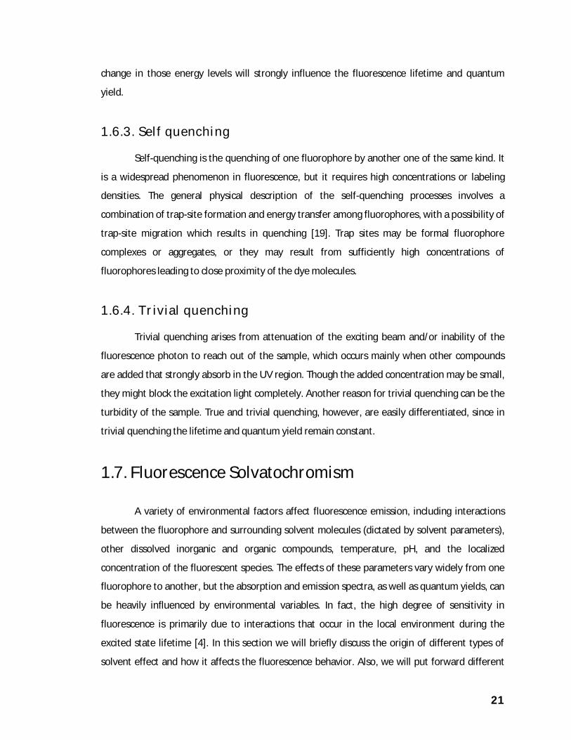
of solvent molecules around the solvated fluorophore (as illustrated in figure 1.9), which
generally has a much larger dipole moment in the excited state than in the ground state.
After the fluorophore has been excited to higher vibrational levels of the first excited
singlet state (S1), excess vibrational energy is rapidly lost to surrounding solvent molecules as
the fluorophore slowly relaxes to the lowest vibrational energy level (occurring in the
picosecond time scale). Solvent molecules assist in stabilizing and further lowering the energy
level of the excited state by re-orienting (termed solvent relaxation) around the excited
fluorophore in a slower process that requires between 10100 ps. This has the effect of
reducing the energy separation between the ground and excited states, which results in a red
shift (to longer wavelengths) of the fluorescence emission. Increasing the solvent polarity
produces a correspondingly larger reduction in the energy level of the excited state, while
decreasing the solvent polarity reduces the solvent effect on the excited state energy level. The
polarity of the fluorophore also determines the sensitivity of the excited state to solvent effects.
Polar and charged fluorophores exhibit a far stronger effect than non-polar fluorophore.
23
Figure 1.9 Fluorophore-solvent excited state interaction.
1.7.2. Specific solvent interaction The general solvent effect discussed above is often depends on the polarizibility of the
solvent (described by the refractive index, n) and the molecular polarizibility resulted from the
re-orientation of the solvent dipole. The later property is a function of the static dielectric
constant, . The mathematical expression is the so called Lippert-Mataga (LM) equation (see
chapter 3 for details). In contrast, specific interactions are produced by one or a few neighboring
molecules, and are determined by the specific chemical properties of both the fluorophore and
solvent. Specific effects can be due to hydrogen bonding, preferential solvation, acid–base
chemistry, or charge-transfer interactions, to name a few. The spectral shifts due to such
specific interactions can be substantial, and if not recognized, limit the detailed interpretation of
fluorescence emission spectra. Specific solvent–fluorophore interactions can often be identified
by examining emission spectra in a variety of solvents. For example, addition of low
concentrations of ethanol, which are too small to alter the bulk properties of the solvent, result
in substantial fluorescence spectral shift in 2-aminonaphthalene [4(a)]. Less than 3% ethanol
causes a shift in the emission maximum from 372 to 400 nm. Increasing the ethanol

24
concentration from 3 to 100% caused an additional shift to only 430 nm. A small percentage of
ethanol (3%) caused almost 50% of the total spectral shift.
Specific solvent–fluorophore interactions can occur in either the ground state or the
excited state. If the interaction only occurred in the excited state, then the polar additive would
not affect the absorption spectra. If the interaction occurs in the ground state, then some
change in the absorption spectrum is expected. The indication for the presence of specific
solvent effect is often seen by a substantial shift in fluorescence peak in presence of trace
amount of protic solvents and/or deviation of LM plot from linearity in protic solvents.
Quantitative interpretation of the specific solvent effect is often difficult and requires a careful
analysis of the fluorescence spectra in a variety of solvents.
1.7.3. Modeling solvent interaction (i) Single - parameter approach
Kosower [20(a)] was the first to use solvatochromism as a probe of solvent polarity that
was based on the solvatochromic shift of 4-methoxycarbonyl-1-ethylpyridinium iodide. Later,
Dimroth and Reichardt [20(b-c)] suggested using betain dyes whose negative solvatochromism is
exceptionally large, which are the basis of famous ET(30) scale. These compounds are considered
as zwitterions having dipole moment of about 15 D in the ground state whereas it is nearly zero
in the excited state. The ET(30) value for a solvent is simply defined as the transition energy for
the longest wavelength absorption band of the dissolved pyridinium-N-phenoxide betaine dye
and normally expressed in kcal mol-1. It has been observed that correlations of solvent-
dependent properties; especially, positions and intensities of absorption and emission bands
with ET(30) scale often follow two distinct lines, one for non-protic solvents and one for protic
solvents. The sensitivity of the betaine dyes to solvent polarity is exceptionally high, but
unfortunately they are not fluorescent. So, the search for polarity-sensitive fluorescent dyes
continues as they offer distinct advantages, particularly in biological studies.
(ii) Multi-parameter approach
In most of the cases, the spectral shift cannot be correlated only in terms of solvent
polarity. Specific interaction of the probe with solvent, for example hydrogen bonding, can also
contribute to the solvent dependent spectral shift. In these case a multi-parameter approach is
preferable and the π* scale of Kamlet and Taft [20(d)] deserves special recognition because it
has been successfully applied to the positions or intensities of maximal absorption in IR, NMR,

25
ESR and UV-Visible absorption and fluorescence spectra and many other physical or chemical
parameters. The advantage of the Kamlet-Taft treatment is to sort out the quantitative role of
properties such as hydrogen bonding. It is remarkable that the π* scale has been established
from the averaged spectral behavior of numerous solutes. It offers the distinct advantage of
taking into account both non-specific (general) and specific interactions.
1.8. Time-resolved Fluorescence Measurement
Time-resolved measurements are widely used in fluorescence spectroscopy, which
contain more information than is available from the steady-state measurement. They were
particularly used for studies of biological macromolecules and increasingly for cellular imaging
[4]. For instance, a protein containing two tryptophan residues cannot be distinguished by the
steady state measurement; whereas, these can be distinguished easily by time-resolved data
giving two decay times. One can also distinguish the presence of static and dynamic quenching
behavior using lifetime measurements [21]. Recently, an important application has been found
in cellular imaging using fluorescence microscopy which can create lifetime images. Time
resolved fluorescence measurements were widely used in two different methods namely - Time
domain (TD) and Frequency domain (FD) methods.
1.8.1. Time-domain measurement In time-domain or pulse fluorimetry, the sample is excited with a pulse of light. The
width of the pulse is made as short as possible, and is preferably much shorter than the
fluorescence decay time (τf) of the sample. The time dependent intensity is measured following
the excitation pulse, and the decay time τf is calculated from the slope of a plot of log I(t) versus
t, or from the time at which the intensity decreases to 1/e of the intensity at t = 0. The intensity
decays are often measured through a polarizer oriented at 54.7o from the vertical z-axis. This
condition is used to avoid the effects of rotational diffusion and/or anisotropy on the intensity
decay.
26
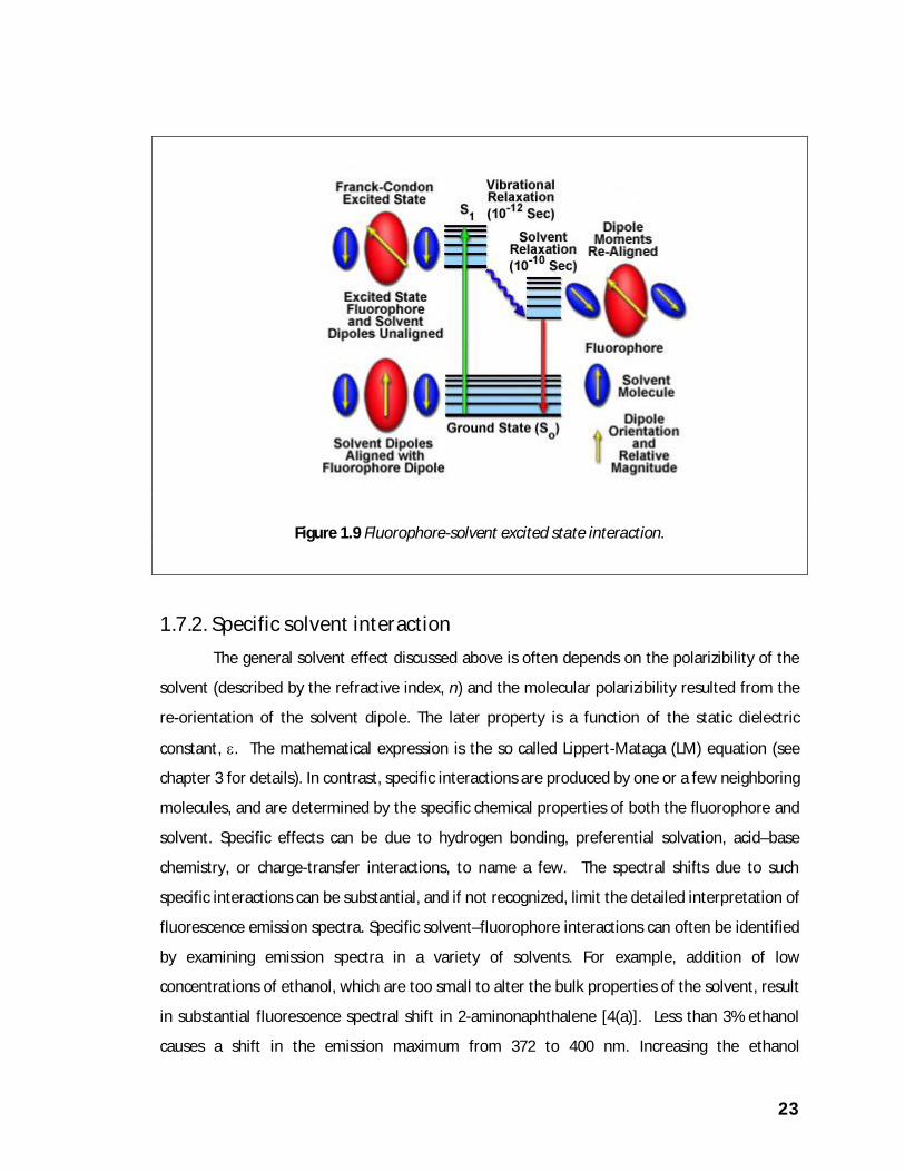
1.8.2. Frequency-domain measurement In frequency domain or phase modulation method, the sample is excited with intensity-
modulated light, typically sine-wave modulation. The intensity of the incident light is varied at a
high frequency typically near 100 MHz, so its reciprocal frequency is comparable to the
reciprocal of decay time. When a fluorescent sample is excited in this manner, the emission is
forced to respond at the same modulation frequency. The lifetime of the fluorophore causes the
emission to be delayed in time relative to the excitation and this delay is measured as a phase
shift (φ), which can be used to calculate the decay time. Magic-angle polarizer conditions are
also used in frequency-domain measurements. The lifetime of the fluorophore also causes a
decrease in the peak-to-peak height of the emission relative to that of the modulated excitation.
The modulation decreases because some of the fluorophores excited at the peak of the
excitation continue to emit when the excitation is at a minimum. The extent to which this occurs
depends on the decay time and light modulation frequency. This effect is called de-modulation,
and can also be used to calculate the decay time. FD measurements typically use both the phase
and modulation information. At present, both time-domain and frequency-domain
measurements are in widespread use.


![[ORAL ARGUMENT NOT SCHEDULED] No. 13-5281 IN THE …](https://img.pdfslide.us/doc/110x75/61d0d07dbc1840220f22294e/oral-argument-not-scheduled-no-13-5281-in-the-.jpg)