Embed Size (px)
Citation preview
Chapter 1
Selective Data Acquisition for MachineLearning
Josh AttenbergNYU Polytechnic Institute, Brooklyn, NY 11201
Prem MelvilleIBM T.J. Watson Research Center, Yorktown Heights, NY 10598
Foster ProvostNYU Stern School of Business, New York, NY 10012
Maytal Saar-TsechanskyRed McCombs School of Business, University of Texas at Austin
1.1 Introduction
In many applications, one must invest effort or money to acquire the data and otherinformation required for machine learning and data mining. Careful selection of the infor-mation to acquire can substantially improve generalization performance per unit cost. Thecostly information scenario that has received the most research attention (see Chapter X)has come to be called ”active learning,” and focuses on choosing the instances for whichtarget values (labels) will be acquired for training. However machine learning applicationsoffer a variety of different sorts of information that may need to be acquired.
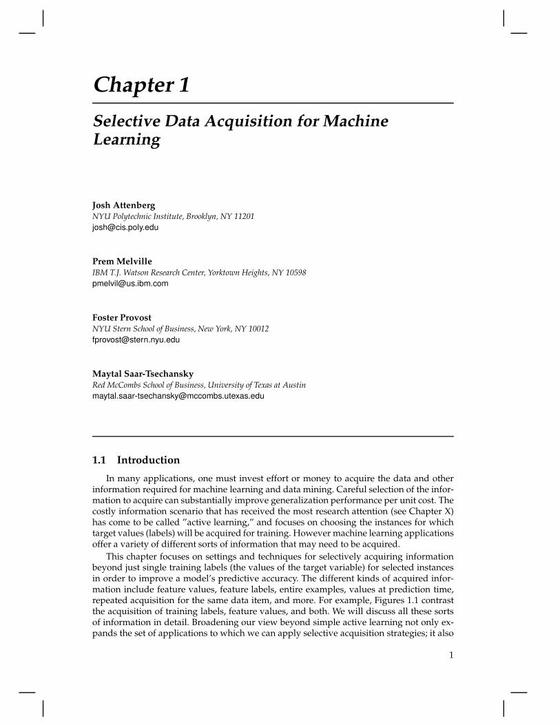
This chapter focuses on settings and techniques for selectively acquiring informationbeyond just single training labels (the values of the target variable) for selected instancesin order to improve a model’s predictive accuracy. The different kinds of acquired infor-mation include feature values, feature labels, entire examples, values at prediction time,repeated acquisition for the same data item, and more. For example, Figures 1.1 contrastthe acquisition of training labels, feature values, and both. We will discuss all these sortsof information in detail. Broadening our view beyond simple active learning not only ex-pands the set of applications to which we can apply selective acquisition strategies; it also
1
2 Cost-sensitive Learning
highlights additional important problem dimensions and characteristics, and reveals fer-tile areas of research that to date have received relatively little attention.
In what follows, we start by presenting two general notions that are employed to helpdirect the acquisition of various sorts of information. The first is to prefer to acquire in-formation for which the current state of modeling is uncertain. The second is to acquireinformation that is estimated to be the most valuable to acquire.
After expanding upon these two overarching notions, we discuss a variety of differentsettings where information acquisition can improve modeling. The purpose of examiningvarious different acquisition settings in some detail is to highlight the different challenges,solutions, and research issues. As just one brief example, distinct from active learning,active acquisition of feature values may have access to additional information, namelyinstances’ labels—which enables different sorts of selection strategies.
More specifically, we examine the acquisition of feature values, feature labels, andprediction-time values. We also examine the specific, common setting where informationis not perfect, and one may want to acquire additional information specifically to deal withinformation quality. For example, one may want to acquire the same data item more thanonce. In addition, we emphasize that it can be fruitful to expand our view of the sortsof acquisition actions we have at our disposal. Providing specific variable values is onlyone sort of information “purchase” we might make. For example, in certain cases, we maybe able to acquire entire examples of a rare class, or distinguishing words for documentclassification. These alternative acquisitions may give a better return on investment formodeling.
Finally, and importantly, most research to date has considered each sort of informationacquisition independently. However, why should we believe that only one sort of infor-mation is missing or noisy? Modelers may find themselves in situations where they needto acquire various pieces of information, and somehow must prioritize the different sortsof acquisition. This has been addressed in a few research papers for pairs of types of in-formation, for example for target labels and feature labels (“active dual supervision”). Weargue that a challenge problem for machine learning and data mining research should beto work toward a unified framework within which arbitrary information acquisitions canbe prioritized, to build the best possible models on a limited budget.
1.2 Overarching principles for selective data acquisition
In general selective data acquisition a learning algorithm can request the value of par-ticular missing data, which is then provided by an oracle at some cost. There may be morethan one oracle, and oracles are not assumed to be perfect. The goal of selective data ac-quisition is to choose to acquire data that is most likely to improve the system’s use-timeperformance on a specified modeling objective in a cost-effective manner. We will use q torefer to the query for a selected piece of missing data. For instance, in traditional activelearning this would correspond to querying for the missing label of a selected instance;while in the context of active feature-value acquisition, q is the request for a missing fea-ture value. We will focus primarily (but not exclusively) on pool-based selective data acqui-sition, where we select a query from a pool of available candidate queries, e.g., the set ofall missing feature-values that can be acquired on request.
Note that in most cases, selection from the pool is performed in epochs, whereby at eachphase, a batch of one or more queries are performed simultaneously. The combinatorial

Selective Data Acquisition for Machine Learning 3
problem of selecting the most useful such batches (and overall data set) from such a pool ofcandidates makes direct optimization an NP-hard problem. Typically, a first order Markovrelaxation is performed, whereby the most promising data are selected greedily one-at-a-time from the pool. While not guaranteeing a globally optimal result set (regardless ofwhat selection criterion is being used), such sequential data access often works well inpractice while making the selection problem tractable.
We begin by discussing two general principles that are applicable for the selective ac-quisition of many different types of data. These overarching principles must be instanti-ated specifically to suit the needs of each acquisition setting. While individual instanti-ations may differ considerably, both principles have advantages and disadvantages thathold in general, which we discuss below. In reviewing these techniques, we often refer tothe familiar active learning setting; we will see how the principles do and do not apply tothe other settings as the chapter unfolds.
1.2.1 Uncertainty Reduction
The most commonly used method for non-uniform sample selection for machine learn-ing is to select data items for which the current model is most uncertain.
This notion is the basis for the most commonly used individual active learning tech-nique, Uncertainty Sampling [44], as well as closely related (and in some cases identical)techniques, such as selecting data points closest to a separating hyperplane, Query-by-Committee and variance reduction [79]. Specifically, with Uncertainty Sampling the activelearner requests labels for examples that the currently held model is least certain abouthow to classify.
Uncertainty reduction techniques are based on the assumption that predictive errorslargely occur in regions of the problem space where predictions are most ambiguous. Theintent is that by providing supplemental information in these regions, model confidencecan be improved, along with predictive performance. Despite the typical reference to theclassic 1994 paper [44], even Uncertainty Sampling itself has become a framework withinwhich different techniques are implemented. For example, exactly how one should mea-sure uncertainty is open to interpretation; the following three calculations of uncertaintyall have been used [79, 55, 78]:
1 − P (y|x) (1.1)
P (y1|x) − P (y2|x) (1.2)
−∑
i
P (yi|x) log(P (yi|x)) (1.3)
where P (y|x) is the highest posterior probability assigned by the classifier to a class, whileP (y1|x) and P (y2|x) are the probabilities assigned to the first and second most probableclasses as predicted by the classifier.
Uncertainty Reduction is widely used with some success in research literature, thoughwe will discuss situations where Uncertainty Reduction fails to make beneficial selections.The same uncertainty-based heuristic can be applied more broadly to acquiring otherforms of data. For instance, when feature-values are missing, one can attempt to imputethe missing values from those that are present, and choose to acquire values where themodel is least certain of the imputed values.
The advantages of Uncertainty Reduction are:
• Evaluating and selecting queries based on uncertainty is computationally efficient inmany settings. For instance, Uncertainty Sampling for training labels only requires

4 Cost-sensitive Learning
applying the classifier to predict the posterior class probabilities of examples in theunlabeled pool. There is no retraining of models required in order to select queries.Note that, in other settings, such as acquiring feature-values, the complexity may beconsiderably higher depending on how one choses to measure uncertainty.
• Uncertainty Reduction techniques are often adopted because of their ease of imple-mentation. For example, Uncertainty Sampling requires computing one of the uncer-tainty scores described above which are simply applications of the existing model inorder to make predictions on an unlabeled instance.
• In the active learning literature, Uncertainty Reduction techniques have been appliedacross many problems with reasonable success.
The disadvantages of Uncertainty Reduction are:
• While often effective in practice, Uncertainty Reduction does not directly attemptto optimize a classifier’s generalization performance. As such it can often choosequeries that may reduce model uncertainty, but not result in improvement on test setpredictions. Notably, when applied to obtaining example labels, Uncertainty Sam-pling is prone to selecting outliers [79]. These could be instances the model is un-certain about, but are not representative of instances in the test set. The selection ofoutliers can be addressed by using the uncertainty scores to form a sampling distri-bution [72, 73]; however, sampling also can reduce the effectiveness of UncertaintyReduction techniques by repeatedly selecting marginally informative examples. Inother settings, Uncertainty Reduction may reduce uncertainty about values that arenot discriminative, such as acquiring values for a feature that is uncorrelated to theclass.
• While Uncertainty Sampling is often favored for ease of implementation, in settingsbeyond the acquisition of single training labels, estimating uncertainty is often notas straightforward. For example, how should you measure the uncertainty of an in-stance label, given a current model and many contradictory labels for the same in-stance from different oracles [82]?
• In general, selective data acquisition assumes that the response to each query comesat a cost. In realistic settings, these costs may vary for each type of acquisition andeven for each query. Notably, some examples are more difficult for humans to la-bel than others, and as such may entail a higher cost in terms of annotation time.Similarly, some features-values are more expensive to obtain than others, e.g., if theyare the result of a more costly experiment. Uncertainty Reduction methods do notnaturally facilitate a meaningful way to trade off costs with potential benefits of eachacquisition. One ad hoc approach of attempting this is to divide the uncertainty scorewith the cost for each query, and make acquisitions in order of the resulting quan-tity [80, 32]. This is a somewhat awkward approach to incorporating costs, as uncer-tainty per unit cost is not necessarily proportional to potential benefit to the resultingmodel.
• As mentioned above, uncertainty can be defined in different ways even for the sametype of acquisition, such as a class label. Different types of acquisitions, such as fea-ture values, require very different measures of uncertainty. Consequently, when con-sidering more than one type of acquisition simultaneously, there is no systematic wayto compare two different measures of uncertainty, since they are effectively on dif-ferent scales. This makes it difficult to construct an Uncertainty Reduction technique
Selective Data Acquisition for Machine Learning 5
that systematically decides which type of information is most beneficial to acquirenext.
1.2.2 Expected Utility
Selecting data that the current model is uncertain about may result in queries thatare not useful in discriminating between classes. An alternative to such uncertainty-basedheuristics is to directly estimate the expected improvement in generalization due to eachquery. In this approach, at every step of selective data acquisition, the next query selectedis the one that will result in the highest estimated improvement in classifier performanceper unit cost. Since the true values of the missing data are unknown prior to acquisition,it is necessary to estimate the potential impact of every query for all possible outcomes. 1
Hence, the decision-theoretic optimal policy is to ask for missing data which, once incorpo-rated into the existing data, will result in the greatest increase in classification performancein expectation. If ωq is the cost of the query q, then its Expected Utility of acquisition can becomputed as
EU(q) =
∫
v
P (q = v)U(q = v)
ωq
(1.4)
where P (q = v) is the probability that query q will take on value v, and U(q = v) is theutility to the model of knowing that q has the value v. This utility can be defined in anyway to represent a desired modeling objective. For example, U could be defined as classi-fication error. In this case, this approach is referred to as Expected Error Reduction. Whenapplied more generally to arbitrary utility functions we refer to such a selection scheme asExpected Utility or Estimated Risk Minimization. Note that, in Equation 1.4 the true values ofthe marginal distribution P (.) and the utility U(.) on the test set is unknown. Instead, em-pirical estimates of these quantities are used in practice. When the missing data can onlytake on discrete values, the expectation can be easily computed by piecewise summationover the possible values. While for continuous values, computation of expected utility canbe performed using Monte Carlo methods.
The advantages of Expected Utility are:
• Since this method is directly trying to optimize the objective on which the model willbe evaluated, it avoids making acquisitions that do not improve this objective evenif it reduces uncertainty or variance in the predictions.
• Incorporating different acquisition costs is also straightforward in this framework.The trade-off of utility versus cost is handled directly, as opposed to relying on anunknown indirect connection between uncertainty and utility.
• This approach is capable of addressing multiple types of acquisition simultaneouslywithin a single framework. Since the measure of utility is independent of the typeof acquisition and only dependent on the resulting classifier, we can estimate the ex-pected utility of different forms of acquisitions in the same manner. For instance, wecan use such an approach to estimate the utility of acquiring class labels and featurevalues in tandem [71]. The same framework can also be instantiated to yield a holis-tic approach to active dual supervision, where the Expected Utility of an instance or
1For instance, in the case of binary classification, the possible outcomes are a positive or negative label for aqueried example.

6 Cost-sensitive Learning
feature label query can be computed and compared on the same scale [2]. By evalu-ating different acquisitions in the same units, and by measuring utility per unit costof acquisition, such a framework facilitates explicit optimization of the trade-offs be-tween the costs and benefits of the different types of acquisitions. between the costsand benefits of the different types of acquisitions.
The disadvantages of Expected Utility are:
• A naive implementation of the Expected Utility framework is computationally in-tractable even for data of moderate dimensionality. The computation of ExpectedUtility (Equation 1.4) requires iterating over all possible outcomes of all candidatequeries. This often means training multiple models for the different values a querymay take on. This combinatorial computational cost can often be prohibitive. Themost common approach to overcome this, at the cost of optimality, is to sub-samplethe set of available queries, and only compute Expected Utility on this smaller can-didate set [71]. This method has also been demonstrated to be feasible for classifiersthat can be rapidly trained incrementally [70]. Additionally, dynamic programmingand efficient data structures can be leveraged to make the computation tractable [8].The computation of the utility of each outcome of each query, while being the bot-tleneck, is also fully parallelizable. As such large-scale parallel computing has thepotential of making the computational costs little more than that of training a singleclassifier.
• As mentioned above, the terms P (.) and U(.) in the Expected Utility computationmust be estimated from available data. However, the choice of methods to use forthese estimations is not obvious. Making the correct choices can be a significant chal-lenge for a new setting, and can make a substantial difference in the effectiveness ofthis approach [71].
• Typically, the estimators used for P (.) and U(.) are based on the pool of availabletraining data, for instance, through cross validation. The available training examplesthemselves are often acquired through an active acquisition process. Here, due tothe preferences of the active process, the distribution of data in the training poolmay differ substantially from that of the native data population and as a result, theestimations of P (.) and U(.) may be arbitrarily inaccurate in the worst case.
• Additionally, it should be noted that despite the emperical risk minimization moniker,Expected Utility methods do not in general yield the globally optimal set of selec-tions. This is due to several simplifications: first, the myopic, sequential acquisitionpolicy mentioned above where the benefit for each individual example is taken inisolation, and second, the utilization of empirical risk as a proxy for actual risks.
1.3 Active feature-value acquisition
In this section we begin by discussing active feature-value acquisition (AFA), the se-lective acquisition of single feature values for training. We then review extensions of thesepolicies for more complex settings in which feature values, different sets thereof, as well asclass labels can be acquired at a cost simultaneously. We discuss some insights on the chal-lenges and effective approaches for these problems as well as interesting open problems.

Selective Data Acquisition for Machine Learning 7
As an example setting for active feature-value acquisition, consider consumers’ ratingsof different products being used as predictors to estimate whether or not a customer islikely to be interested in an offer for a new product. At any given time, only a subset ofany given consumer’s “true” ratings of her prior purchases are available, and thus manyfeature values are missing, potentially undermining inference. To improve this inference,it is possible to offer consumers incentives so as to reveal their preferences—for example,rating other prior purchases. Thus, it is useful to devise an intelligent acquisition policyto select which products and which consumers are most cost-effective to acquire. Similarscenarios arise in a variety of other domains, including when databases are being usedto estimate the likelihood of success of alternative medical treatments. Often the featurevalues of some predictors, such as of medical tests, are not available; furthermore, theacquisition of different tests may incur different costs.
This general active feature-value acquisition setting, illustrated in Figure 1.1(b), differsfrom active learning in several important ways. First, policies for acquiring training labelsassign one value to an entire prospective instance acquisition. Another related distinctionis that the impact on induction from obtaining an entire instance may require a less pre-cise measure to that required to estimate the impact from acquiring merely a single featurevalue. In addition, having multiple missing feature values gives rise to a myriad of set-tings regarding the level of granularity at which feature values can be acquired and thecorresponding cost [102, 47, 57, 56, 38]. For example, in some applications, such as whenacquiring consumers’ demographic and lifestyle data from syndicated data providers, onlythe complete set of all feature values can be purchased at a fixed cost. In other cases, suchas the recommender systems and treatment effectiveness tasks above, it may be possibleto purchase the value of a single variable, such as by running a medical test. And thereare intermediate cases, such as when different subsets (e.g., a battery of medical tests) canbe acquired as a bundle. Furthermore, different sets may incur different costs; thus, whilevery few policies do so, it is beneficial to consider such costs when prioritizing acquisition.In the remainder of this section, we discuss how we might address some of these problemsettings, as well as interesting open challenges.
A variety of different policies can be envisioned for the acquisition of individual featurevalues at a fixed cost, following the Expected Utility framework we discussed in Section1.2 and [47, 56, 71]. As such, Expected Utility AFA policies aim to estimate the expectedbenefit from an acquisition by the change in some loss/gain function in expectation.For feature value acquisitions the expected utility framework has several important ad-vantages, but also some limitations. Because different features (such as medical tests) arevery likely to incur different costs perhaps the most salient advantage for AFA is the abil-ity to incorporate cost information when prioritizing acquisitions. The Expected Utilityframework also allows us to prioritize among acquisitions of individual features as wellas different sets thereof. However, the expected value framework would guarantee the ac-quisition of the optimal single feature value in expectation, only if the true distributionsof values for each missing feature were known, and the loss/gain function, U , were tocapture the actual change in the model’s generalization accuracy following an acquisition.In settings where many feature values are missing these estimations may be particularlychallenging. For example, empirical estimation of the model’s generalization performanceover instances with many missing values may not accurately approximate the magnitudeor even the direction of change in generalization accuracy. Perhaps a more important con-sideration regarding the choice of gain function, U , for feature value acquisition is the se-quential, myopic nature of these policies. Similar to most information acquisition policies,if multiple features are to be acquired, a myopic policy, which aims to estimate the benefitfrom each prospective acquisition in isolation, is not guaranteed to identify the optimalset of acquisitions, even if the estimations listed above were precise. This is because the

8 Cost-sensitive Learning
expected contribution of an individual acquisition is estimated with respect to the currenttraining data, irrespective of other acquisitions which will be made. Interestingly, due tothis myopic property, selecting the acquisition which yields the best estimated improve-ment in generalization accuracy often does not yield the best results; rather, other measureshave been shown to be empirically more effective [71]—for example, log gain. Specifically,
when a model is induced from a training set T , let P (ck|xi) be the probability estimatedby the model that instance xi belongs to class ck; and I is an indicator function such thatI(ck, xi) = 1 if ck is the correct class for xi and I(ck, xi) = 0, otherwise. Log Gain (LG) isthen defined as:
LG(xi) = −
K∑
k=1
I(ck, xi) log P (ck|xi) (1.5)
Notably, LG is sensitive to changes in the model’s estimated probability of the correctclass. As such, this policy promotes acquisitions which increase the likelihood of correctclass prediction, once other values are acquired.
We have discussed the computational cost which the Expected Utility framework en-tails and the need to reduce the consideration set to a small subset of all prospective ac-quisitions. For AFA, drawing from the set of prospective acquisitions uniformly at ran-dom [71] may be used; however, using a fast heuristics to identify feature values that arelikely to be particularly informative per unit cost can be more effective. For example, auseful heuristic is to draw a subset of prospective acquisitions based on the correspondingfeatures’ predictive values [71] or to prefer acquisitions from particularly informative in-stances [56].
A related setting, illustrated in Figure 1.1(c), is one in which for all instances the samesubset of feature values are known, and the subset of all remaining feature values can beacquired at a fixed cost. Henceforth, we refer to this setting as instance completion. Undersome conditions, this problem bears strong similarity to the active learning problem. Forexample, consider a version of this problem in which only instances with complete featurevalues are used for induction [102, 103]. If the class labels of prospective training exam-ples are unknown or are otherwise not used to select acquisition, this problem becomesvery similar to active learning in that the value from acquiring a complete training in-stance must be estimated. For example, we can use measures of prediction uncertainty (cf.,section 1.2 to prioritize acquisitions [103].
Note however that the active feature-value acquisition setting may have additional in-formation that can be brought to bear to aid in selection: the known class labels of prospec-tive training examples. The knowledge of class labels can lead to selection policies thatprefer to acquire features for examples on which the current model makes mistakes [57].An extreme version of the instance completion problem is when there are no known fea-ture values and the complete feature set can be acquired as a bundle for fixed cost (seeSection 1.7 below).
Acquiring feature values and class labelsWe noted earlier that an important benefit of the AFA Expected Utility framework is
that it allows comparing among the benefits from acquiring feature values, sets thereof,as well as class labels—and thus can consider selecting these different sorts of data si-multaneously [71]. This setting is shown in Figure 1.1(d). Note, however, that consideringdifferent types of acquisitions simultaneously also presents new challenges. In particular,recall the need for a computationally fast heuristic to select a subset of promising prospec-tive acquisitions to be subsequently estimated by the Expected Utility policy. Assuming
Selective Data Acquisition for Machine Learning 9
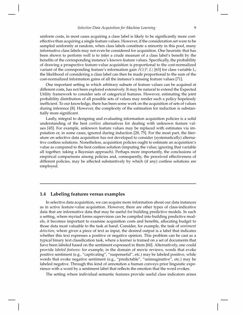
uniform costs, in most cases acquiring a class label is likely to be significantly more cost-effective than acquiring a single feature values. However, if the consideration set were to besampled uniformly at random, when class labels constitute a minority in this pool, manyinformative class labels may not even be considered for acquisition. One heuristic that hasbeen shown to perform well is to infer a crude measure of a class label’s benefit by thebenefits of the corresponding instance’s known feature values. Specifically, the probabilityof drawing a prospective feature-value acquisition is proportional to the cost-normalizedvariant of the corresponding feature’s information gain IG(F, L) [63] for class variable L;the likelihood of considering a class label can then be made proportional to the sum of thecost-normalized information gains of all the instance’s missing feature values [71].
One important setting in which arbitrary subsets of feature values can be acquired atdifferent costs, has not been explored extensively. It may be natural to extend the ExpectedUtility framework to consider sets of categorical features. However, estimating the jointprobability distribution of all possible sets of values may render such a policy hopelesslyinefficient. To our knowledge, there has been some work on the acquisition of sets of valuesduring inference [8]. However, the complexity of the estimation for induction is substan-tially more significant.
Lastly, integral to designing and evaluating information acquisition policies is a solidunderstanding of the best costless alternatives for dealing with unknown feature val-ues [45]. For example, unknown feature values may be replaced with estimates via im-putation or, in some cases, ignored during induction [28, 75]. For the most part, the liter-ature on selective data acquisition has not developed to consider (systematically) alterna-tive costless solutions. Nonetheless, acquisition policies ought to estimate an acquisition’svalue as compared to the best costless solution (imputing the value; ignoring that variableall together; taking a Bayesian approach). Perhaps more importantly, the conclusions ofempirical comparisons among policies and, consequently, the perceived effectiveness ofdifferent policies, may be affected substantively by which (if any) costless solutions areemployed.
1.4 Labeling features versus examples
In selective data acquisition, we can acquire more information about our data instancesas in active feature-value acquisition. However, there are other types of class-indicativedata that are informative data that may be useful for building predictive models. In sucha setting, where myriad forms supervision can be compiled into building predictive mod-els, it becomes important to examine acquisition costs and benefits, allocating budget tothose data most valuable to the task at hand. Consider, for example, the task of sentimentdetection, where given a piece of text as input, the desired output is a label that indicateswhether this text expresses a positive or negative opinion. This problem can be cast as atypical binary text classification task, where a learner is trained on a set of documents thathave been labeled based on the sentiment expressed in them [60]. Alternatively, one couldprovide labeled features: for example, in the domain of movie reviews, words that evokepositive sentiment (e.g., “captivating”, “suspenseful”, etc.) may be labeled positive, whilewords that evoke negative sentiment (e.g., “predictable”, “unimaginative”, etc.) may belabeled negative. Through this kind of annotation a human conveys prior linguistic expe-rience with a word by a sentiment label that reflects the emotion that the word evokes.
The setting where individual semantic features provide useful class indicators arises

10 Cost-sensitive Learning
Labels
Labels
Labels
Labels
Feature Values Feature Values
Feature Values Feature Values
(a) Active Learning (b) Active Feature Value Acquisition
(c) Instance Completion AFA (d) Active Information Acquisition
Instances
Instances
Instances
Instances
FIGURE 1.1: Different Data Acquisition Settings
broadly, notably in Natural Language Processing tasks where, in addition to labeled doc-uments, it is possible to provide domain knowledge in the form of words or phrases [100]or more sophisticated linguistic features that associate strongly with a class. Such featuresupervision can greatly reduce the number of labels required to build high-quality classi-fiers [24, 84, 54]. In general, example and feature supervision are complementary, ratherthan redundant. As such they can also be used together. This general setting of learningfrom both labels on examples and features is referred to as dual supervision [84].
In this section we provide a brief overview of learning from labeled features, as well aslearning both from labeled features and labeled examples. We will also discuss the chal-lenges of active learning in these settings, and some approaches to overcome them.
1.4.1 Learning from feature labels
Providing feature-class associations through labeling features can be viewed as oneapproach to expressing background, prior or domain knowledge about a particular su-pervised learning task. Methods to learn from such feature labels can be divided into ap-proaches that use labeled features along with unlabeled examples, and methods that useboth labeled features and examples. Since, we focus primarily on text classification in this
Selective Data Acquisition for Machine Learning 11
section, we will use words and documents interchangeably with features and examples. How-ever, incorporating background knowledge into learning has also been studied outside thecontext of text classification, as in knowledge-based neural networks [90] and knowledge-based SVMs [29, 42].
Labeled features and unlabeled examples
A simple way to utilize feature supervision is to use the labels on features to label ex-amples, and then use an existing supervised learning algorithm to build a model. Considerthe following straightforward approach. Given a representative set of words for each class,create a representative document for each class containing all the representative words. Thencompute the cosine similarity between unlabeled documents and the representative docu-ments. Assign each unlabeled document to the class with the highest similarity, and thentrain a classifier using these pseudo-labeled examples. This approach is very convenient as itdoes not require devising a new model, since it can effectively leverage existing supervisedlearning techniques such as Naıve Bayes [46]. Given that it usually take less time to label aword than it takes to label a document [24], this is a cost-effective alternative.
An alternative to approaches of generating and training with pseudo-labeled examples,is to directly use the feature labels to constrain model predictions. For instance, a label y
for feature xi can be translated into a soft constraint, P (y|xi) > 0.9, in a multinomial logis-tic regression model [24]. Then the model parameters can be optimized to minimize somedistance, e.g. Kullback-Leibler divergence from these reference distributions.
Dual Supervision
In dual supervision models, labeled features are used in conjunction with labeled ex-amples. Here too, labeled features can be used to generate pseudo-labeled examples, eitherby labeling unlabeled examples [97] or re-labeling duplicates of the training examples [77].These pseudo-labeled examples can be combined with the given labeled examples, usingweights to down-weight prior knowledge when more labeled examples are available. Suchmethods can be implemented within existing frameworks, such as boosting logistic regres-sion [77], and weighted margin support vector machines [97].
Generating pseudo-labeled examples is an easy way to leverage feature labels withinthe traditional supervised learning framework based on labeled examples. Alternativelyone can incorporate both forms of supervision directly into one unified model [54, 84].Pooling Multinomials is one such classifier, which builds a generative model that explainsboth labeled features and examples. In Pooling Multinomials unlabeled examples are clas-sified just as in multinomial Naıve Bayes classification [52], by predicting the class withthe maximum likelihood, given by argmaxcj
P (cj)∏
i P (wi|cj); where P (cj) is the priorprobability of class cj , and P (wi|cj) is the probability of word wi appearing in a documentof class cj . In the absence of background knowledge about the class distribution, the classpriors P (cj) are estimated solely from the training data. However, unlike regular NaıveBayes, the conditional probabilities P (wi|cj) are computed using both the labeled exam-ples and the set of labeled features. Given two models built using labeled examples andlabeled features, the multinomial parameters of such models are aggregated through a con-vex combination, P (wi|cj) = αPe(wi|cj)+ (1−α)Pf(wi|cj); where Pe(wi|cj) and Pf (wi|cj)represent the probability assigned by using the example labels and feature labels respec-tively, and α is a weight indicating the level of confidence in each source of information.At the crux of this framework is the generative labeled-features model, which assumesthat the feature-class associations provided by human experts are implicitly arrived at byexamining many latent documents of each class. This assumption translates in into severalconstraints on the model parameter, which allows one to exactly derive the conditionaldistributions Pf (wi|cj) that would generate the latent documents [54].
12 Cost-sensitive Learning
1.4.2 Active Feature Labeling
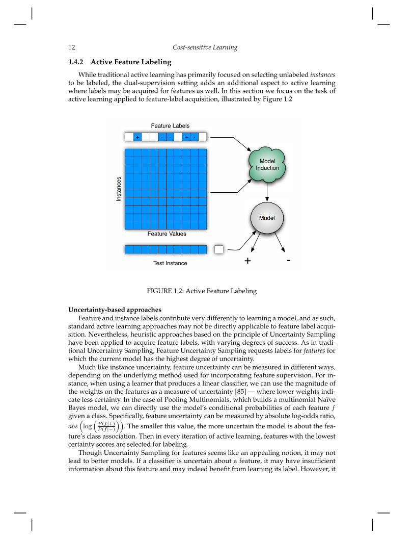
While traditional active learning has primarily focused on selecting unlabeled instancesto be labeled, the dual-supervision setting adds an additional aspect to active learningwhere labels may be acquired for features as well. In this section we focus on the task ofactive learning applied to feature-label acquisition, illustrated by Figure 1.2
+ - - + -
Instances
Test Instance
Feature Labels
Model
Model
Induction
+ -
Feature Values
FIGURE 1.2: Active Feature Labeling
Uncertainty-based approaches
Feature and instance labels contribute very differently to learning a model, and as such,standard active learning approaches may not be directly applicable to feature label acqui-sition. Nevertheless, heuristic approaches based on the principle of Uncertainty Samplinghave been applied to acquire feature labels, with varying degrees of success. As in tradi-tional Uncertainty Sampling, Feature Uncertainty Sampling requests labels for features forwhich the current model has the highest degree of uncertainty.
Much like instance uncertainty, feature uncertainty can be measured in different ways,depending on the underlying method used for incorporating feature supervision. For in-stance, when using a learner that produces a linear classifier, we can use the magnitude ofthe weights on the features as a measure of uncertainty [85] — where lower weights indi-cate less certainty. In the case of Pooling Multinomials, which builds a multinomial NaıveBayes model, we can directly use the model’s conditional probabilities of each feature f
given a class. Specifically, feature uncertainty can be measured by absolute log-odds ratio,
abs(
log(
P (f |+)P (f |−)
))
. The smaller this value, the more uncertain the model is about the fea-
ture’s class association. Then in every iteration of active learning, features with the lowestcertainty scores are selected for labeling.
Though Uncertainty Sampling for features seems like an appealing notion, it may notlead to better models. If a classifier is uncertain about a feature, it may have insufficientinformation about this feature and may indeed benefit from learning its label. However, it

Selective Data Acquisition for Machine Learning 13
is also quite likely that a feature has a low certainty score because it does not carry muchdiscriminative information about the classes. For instance, in the context of sentiment de-tection, one would expect that neutral/non-polar words will appear to be uncertain words.For example, words such as “the” which are unlikely to help in discriminating betweenclasses, are also likely to be considered the most uncertain. In such cases, Feature Uncer-tainty ends up squandering queries on such words ending up with performance inferior torandom feature queries. What works significantly better in practice is Feature Certainty, thatacquires labels for features in descending order of the uncertainty scores [85, 58]. Alternativeuncertainty-based heuristics have also been used with different degrees of success [25, 31].
Expected feature utility
Selecting features that the current model is uncertain about may results in queries thatare not useful in discriminating between classes. On the other hand, selecting the most cer-tain features is also suboptimal, since queries may be wasted simply confirming confidentpredictions, which is of limited utility to the model. An alternative to such certainty-basedheuristics, is to directly estimate the expected value of acquiring each feature label. Thiscan be done by instantiating the Expected Utility framework described in Section 1.2.2,for this setting. This results in the decision-theoretic optimal policy, which is to ask forfeature labels which, once incorporated into the data, will result in the highest increase inclassification performance in expectation.
More precisely, if fj is the label of the j-th feature, and qj is the query for this feature’slabel, then the Expected Utility of a feature query qj can be computed as:
EU(qj) =
K∑
k=1
P (fj = ck)U(fj = ck) (1.6)
Where P (fj = ck) is the probability that fj will be labeled with class ck, and U(fj = ck) isthe utility to the model of knowing that fj has the label ck. As in other applications of thisframework, the true values of these two quantities are unknown, and the main challengeis to accurately estimate these quantities from the data currently available.
A direct way to estimate the utility of a feature label is to measure expected classifica-tion accuracy. However, small changes in the probabilistic model that result from acquiringa single additional feature label may not be reflected by a change in accuracy. As in activefeature-value acquisition (see Section 1.3) one can use a finer-grained measure of classifierperformance, such as Log Gain defined in Equation 1.5. Then the utility of a classifier, U ,can be measured by summing the Log Gain for all instances in the training set.
In Eq. 1.6, apart from the measure of utility, we also do not know the true probabilitydistribution of labels for the feature under consideration. This too can be estimated fromthe training data, by seeing how frequently the word appears in documents of each class.For Pooling Multinomials, one can use the model parameters to estimate the feature label
distribution, P (fj = ck) =P (fj |ck)
P
Kk=1
P (fj |ck). Given the estimated values of the feature-label
distribution and the utility of a particular feature query outcome, we can now estimate theExpected Utility of each unknown feature, selecting the features with the highest ExpectedUtility for labeling.
As in other settings, this approach can be computationally intensive if Expected Utilityestimation is performed on all unknown features. In the worst case this requires buildingand evaluating models for each possible outcome of each unlabeled feature. In a settingwith m features and K classes, this approach requires training O(mK) classifiers. How-ever, the complexity of the approach can be significantly alleviated by only applying Ex-pected Utility evaluation to a sub-sample of all unlabeled features. Given a large number

14 Cost-sensitive Learning
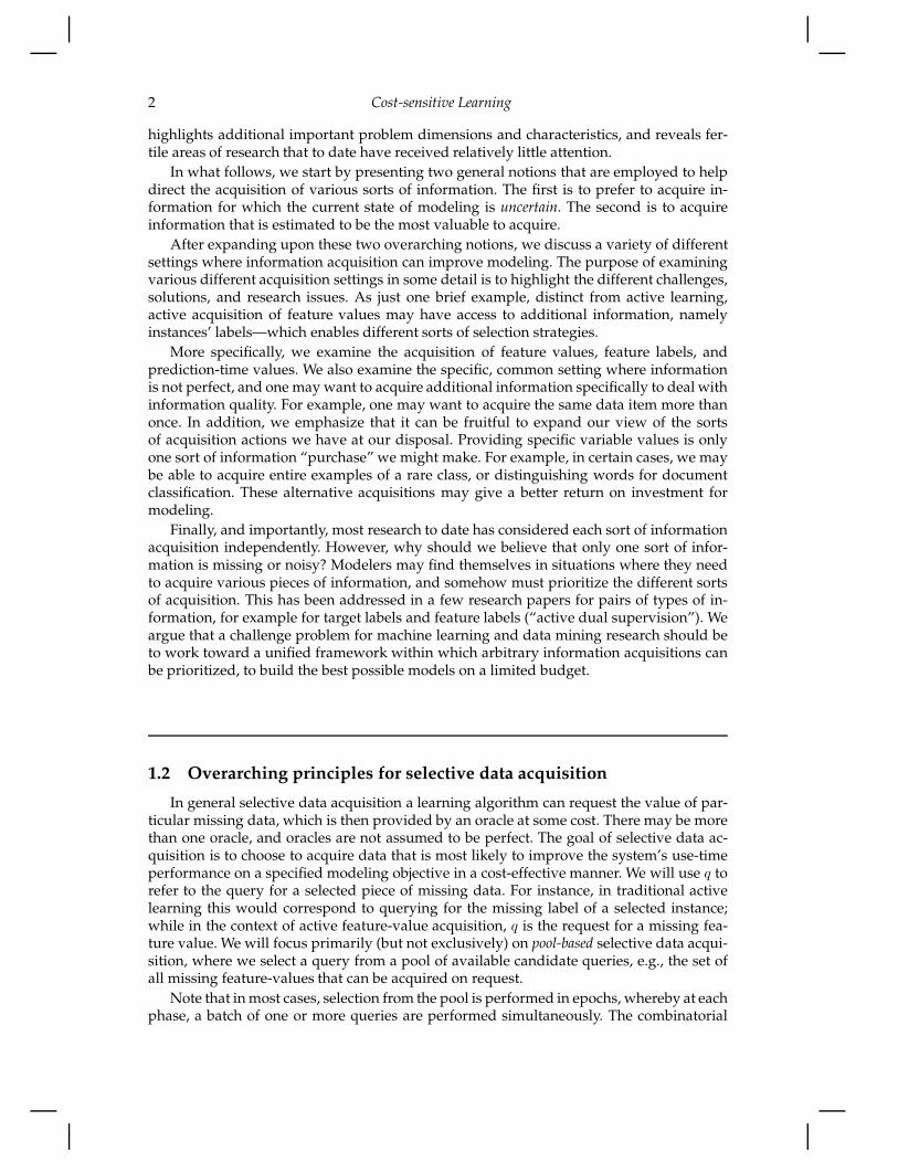
of features with no true class labels, selecting a sample of available features uniformly atrandom may be sub-optimal. Instead one can subsample features based on a fast and effec-tive heuristic like Feature Certainty [85]. Figure 1.3 shows the typical advantage one cansee using such a decision-theoretic approach versus uncertainty-based approaches.
50
55
60
65
70
75
0 50 100 150 200 250 300 350 400
Acc
urac
y
Number of queries
Feature UtilityFeature CertaintyRandom Feature
Feature Uncertainty
FIGURE 1.3: Comparison of different approaches for actively acquiring feature labels, asdemonstrated on the Pooling Multinomials classifier applied to the Movies [60] data set.
1.4.3 Active Dual Supervision
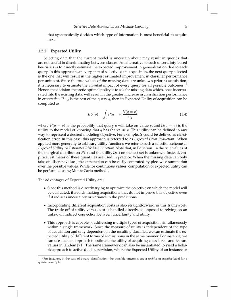
Since dual supervision makes it possible to learn from labeled examples and labeledfeatures simultaneously, one would expect more labeled data of either form to lead tomore accurate models. Fig. 1.4 illustrates the influence of increased number of instancelabels and feature labels independently, and also in tandem. The figure presents an em-pirical comparison of three schemes: Instances-then-features, Features-then-instances, andPassive Interleaving. As the name suggests, Instances-then-features, provides labels for ran-domly selected instances until all instances have been labeled, and then switches to label-ing features. Similarly, Features-then-instances acquires labels for randomly selected featuresfirst and then switches to getting instance labels. In Passive Interleaving we probabilisticallyswitch between issuing queries for randomly chosen instance and feature labels.
We see from Fig. 1.4 that fixing the number of labeled features, and increasing the num-ber of labeled instances steadily improves classification accuracy. This is what one wouldexpect from traditional supervised learning curves. More interestingly, the results also in-dicate that we can fix the number of instances, and improve accuracy by labeling morefeatures. Finally, results on Passive Interleaving show that though both feature labels andexample labels are beneficial by themselves, dual supervision which exploits the inter-action of examples and features does in fact benefit from acquiring both types of labelsconcurrently.
In the sample results above, we selected instances and/or features to be labeled uni-formly at random. Based on previous work in active learning one would expect that we canselect instances to be labeled more efficiently, by having the learner decide which instancesit is most likely to benefit from. The results in the previous section show that actively select-ing features to be labeled is also beneficial. Furthermore, the Passive Interleaving results

Selective Data Acquisition for Machine Learning 15
50
55
60
65
70
75
80
85
90
0 1000 2000 3000 4000 5000 6000 7000
Acc
urac
y
Number of queries
Instances-then-featuresFeatures-then-instances
Passive Interleaving
FIGURE 1.4: Comparing the effect of instance and feature label acquisition in dual super-vision. At the end of the learning curves, each method has labels for all available instancesand features; and as such, the last points of all three curves are identical.
suggest that an ideal active dual supervision scheme would actively select both instancesand features for labeling. This setting is illustrated in Figure 1.5.
One could apply an Uncertainty Sampling approach to this problem. However, thoughuncertainty scores can be used to order examples or features by themselves, there is noprincipled way to compare an uncertainty score computed for an example with a score fora feature. This is because these scores are based on different heuristics for examples andfeatures, and are not in comparable units. One alternative is to apply uncertainty-basedactive learning schemes to select labels for examples and features separately. Then, at eachiteration of active dual supervision, randomly choose to acquire a label for either an ex-ample or feature, and probe the corresponding active learner. Such an Active Interleavingapproach is in general more effective than the active learning of either instances or featuresin isolation [85]. While easy to implement, and effective in practice, this approach is depen-dent on the ad hoc selection of the interleave probability parameter, which determines howfrequently to probe for an example versus a feature label. This approach is indeed quitesensitive to the choice of this interleave probability [85]. An ideal active scheme should,instead, be able to assess if an instance or feature would be more beneficial at each step,and select the most informative instance or feature for labeling.
Fortunately, the Expected Utility method is very flexible, capable of addressing bothtypes of acquisition within a single framework. Since the measure of utility is independentof the type of supervision and only dependent on the resulting classifier, we can estimatethe expected utility of different forms of acquisitions in the same manner. This yields aholistic approach to active dual supervision, where the Expected Utility of an instance orfeature label query, q, can be computed as
EU(q) =
K∑
k=1
P (q = ck)U(q = ck)
ωq
(1.7)
where ωq is the cost of the query q, P (q = ck) is the probability of the instance or featurequeried being labeled as class ck, and utility U can be computed as in Eq. 1.5. By evaluating

16 Cost-sensitive Learning
-
+
+
-
+
+ - - + -
Instances
Instance
Labels
Test Instance
Feature Labels
Dual-
Trained
Model
Model
Induction
+ -
Feature Values
FIGURE 1.5: Active Dual Supervision
instances and features in the same units, and by measuring utility per unit cost of acquisi-tion, such a framework facilitates explicit optimization of the trade-offs between the costsand benefits of the different types of acquisitions. As with Feature Utility, query selectioncan be sped up by sub-sampling both examples and features, and evaluating the ExpectedUtility on this candidate set. It has been demonstrated that such a holistic approach doesindeed effectively manage the trade-offs between the costs and benefits of the differenttypes of acquisitions, to deterministically select informative examples or features for label-ing [2]. Figure 1.6 shows the typical improvements of this unified approach to active dualsupervision over active learning for only example or feature labels.
1.5 Dealing with noisy acquisition
We have discussed various sorts of information that can be acquired (actively) for train-ing statistical models. Most of the research on active/selective data acquisition either hasassumed that the acquisition sources provide perfect data, or has ignored the quality ofthe data sources. Let’s examine this more critically. Here, let’s call the values that we willacquire “labels”. In principle these could be values of the dependent variable (traininglabels), feature labels, feature values, etc., although the research to which we refer has fo-cused exclusively on training labels.
In practical settings, it may well be that the labeling is not 100% reliable—due to im-perfect sources, contextual differences in expertise, inherent ambiguity, noisy informationchannels, or other reasons. For example, when building diagnostic systems, even expertsare found to disagree on the “ground truth”: “no two experts, of the 5 experts surveyed,agreed upon diagnoses more than 65% of the time. This might be evidence for the dif-ferences that exist between sites, as the experts surveyed had gained their expertise atdifferent locations. If not, however, it raises questions about the correctness of the expert

Selective Data Acquisition for Machine Learning 17
0 50 100 150 200 250 300 350 40050
55
60
65
70
75
80
Number of Queries
Acc
urac
y
Passive InterleavingInstance UncertaintyFeature UtilityExpected Utility
FIGURE 1.6: The effectiveness of Expected Utility instantiated for active dual supervision,compared to alternative label acquisition strategies.
data” [62]. The quality of selectively acquired data recently has received greatly increasedattention, as modelers increasingly have been taking advantage of low-cost human re-sources for data acquisition. Micro-outsourcing systems, such as Amazon’s MechanicalTurk (and others) are being used routinely to provide data labels. The cost of labeling us-ing such systems is much lower than the cost of using experts to label data. However, withthe lower cost can come lower quality.
Surveying all the work on machine learning and data mining with noisy data is be-yond the scope of this chapter. The interested reader might start with some classic pa-pers [86, 51, 83]. We will discuss some work that has addressed strategies for the acquisitionof data specifically from noisy sources to improve data quality for machine learning anddata mining (the interested reader should also see work on information fusion [18].
+
Instances
+
+-
-
-
+-
+
Oracle-++-+- Imperfect
Oracles
Feature Values Labels
FIGURE 1.7: Multiple Noisy Oracles

18 Cost-sensitive Learning
0.4
0.5
0.6
0.7
0.8
0.9
1.0
0 40 80 120 160 200 240 280
RO
C A
rea
Number of examples (Mushroom)
q=0.5
q=0.6
q=0.7
q=0.8
q=0.9
q=1.0
FIGURE 1.8: Learning curves under different quality levels of training data (q is the prob-ability of a label being correct).
1.5.1 Multiple label acquisition: round-robin techniques
If data acquisition costs are relatively low, a natural strategy for addressing data qualityis to acquire the same data point multiple times, as illustrated in Figure 1.7. This assumesthat there is at least some independence between repeated acquisitions of the same datapoint, with the most clean-cut case being that each acquisition is an independent randomdraw of the value of the variable, from some noisy labeling process. We can define the classof generalized round-robin (GRR) labeling strategies. [82]: request a label for the data pointthat currently has the fewest labels. Depending on the process by which the rest of the dataare acquired/selected, generalized round-robin can be instantiated differently. If there isone fixed set of data points to be labeled, GRR becomes the classic fixed round-robin: cyclethrough the data points in some order obtaining another label for each. If a new data pointis presented every k labels, then GRR becomes the common strategy of acquiring a fixednumber of labels on each data point [88, 87].
Whether one ought to engage in round-robin repeated labeling depends on several fac-tors [82], which are clarified by Figure 1.8. Here we see a set of learning curves2 for theclassic mushroom classification problem from the UCI repository [12]. The mushroom do-main provides a useful illustration because with perfect labels and a moderate amount oftraining, predictive models can achieve perfect classification. Thus, we can examine theeffect of having noisy labels and multiple labels. The several curves in the figure showlearning curves for different labeling qualities—here simply the probability that a labelerwill give the correct label for this binary classification problem. As the labeler quality de-teriorates, not only does the generalization performance suffer, but importantly the rate-of-change of the generalization performance as a function of the number of labeled datasuffers markedly.
Thus, we can summarize the conditions under which we should consider repeatedlabeling [82]:
1. What is the relative cost of acquiring labels for data points, as compared to the cost of
2Generalization accuracy estimated using cross-validation with a classification tree model.
Selective Data Acquisition for Machine Learning 19
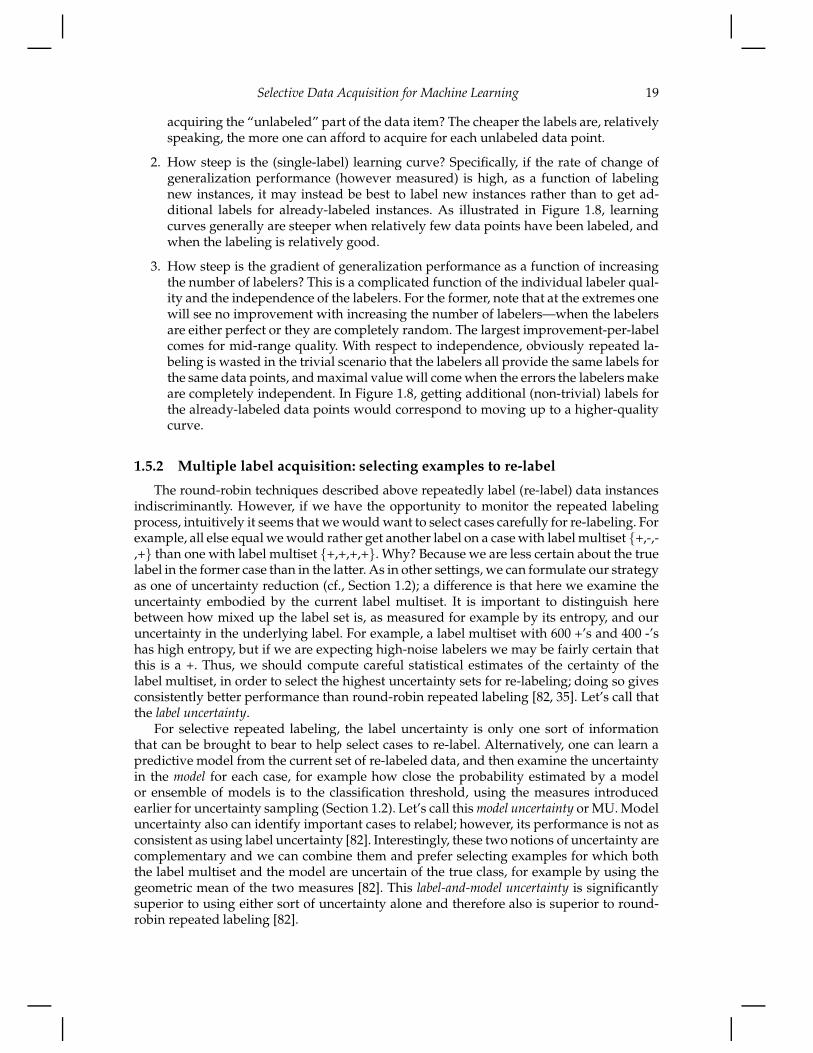
acquiring the “unlabeled” part of the data item? The cheaper the labels are, relativelyspeaking, the more one can afford to acquire for each unlabeled data point.
2. How steep is the (single-label) learning curve? Specifically, if the rate of change ofgeneralization performance (however measured) is high, as a function of labelingnew instances, it may instead be best to label new instances rather than to get ad-ditional labels for already-labeled instances. As illustrated in Figure 1.8, learningcurves generally are steeper when relatively few data points have been labeled, andwhen the labeling is relatively good.
3. How steep is the gradient of generalization performance as a function of increasingthe number of labelers? This is a complicated function of the individual labeler qual-ity and the independence of the labelers. For the former, note that at the extremes onewill see no improvement with increasing the number of labelers—when the labelersare either perfect or they are completely random. The largest improvement-per-labelcomes for mid-range quality. With respect to independence, obviously repeated la-beling is wasted in the trivial scenario that the labelers all provide the same labels forthe same data points, and maximal value will come when the errors the labelers makeare completely independent. In Figure 1.8, getting additional (non-trivial) labels forthe already-labeled data points would correspond to moving up to a higher-qualitycurve.
1.5.2 Multiple label acquisition: selecting examples to re-label
The round-robin techniques described above repeatedly label (re-label) data instancesindiscriminantly. However, if we have the opportunity to monitor the repeated labelingprocess, intuitively it seems that we would want to select cases carefully for re-labeling. Forexample, all else equal we would rather get another label on a case with label multiset {+,-,-,+} than one with label multiset {+,+,+,+}. Why? Because we are less certain about the truelabel in the former case than in the latter. As in other settings, we can formulate our strategyas one of uncertainty reduction (cf., Section 1.2); a difference is that here we examine theuncertainty embodied by the current label multiset. It is important to distinguish herebetween how mixed up the label set is, as measured for example by its entropy, and ouruncertainty in the underlying label. For example, a label multiset with 600 +’s and 400 -’shas high entropy, but if we are expecting high-noise labelers we may be fairly certain thatthis is a +. Thus, we should compute careful statistical estimates of the certainty of thelabel multiset, in order to select the highest uncertainty sets for re-labeling; doing so givesconsistently better performance than round-robin repeated labeling [82, 35]. Let’s call thatthe label uncertainty.
For selective repeated labeling, the label uncertainty is only one sort of informationthat can be brought to bear to help select cases to re-label. Alternatively, one can learn apredictive model from the current set of re-labeled data, and then examine the uncertaintyin the model for each case, for example how close the probability estimated by a modelor ensemble of models is to the classification threshold, using the measures introducedearlier for uncertainty sampling (Section 1.2). Let’s call this model uncertainty or MU. Modeluncertainty also can identify important cases to relabel; however, its performance is not asconsistent as using label uncertainty [82]. Interestingly, these two notions of uncertainty arecomplementary and we can combine them and prefer selecting examples for which boththe label multiset and the model are uncertain of the true class, for example by using thegeometric mean of the two measures [82]. This label-and-model uncertainty is significantlysuperior to using either sort of uncertainty alone and therefore also is superior to round-robin repeated labeling [82].

20 Cost-sensitive Learning
Although model uncertainty uses the same measures as Uncertainty Sampling, thereis a major difference. The difference is that to compute MU the model is applied back tothe cases from which it was trained; mislabeled cases get systematically higher model un-certainty scores [35]. Thus, model uncertainty actually is more closely akin to methods forfinding labeling errors [14]: it selects cases to label because they are mislabeled, in a “self-healing” process, rather than because the examples are going to improve a model in theusual active-learning sense. This can be demonstrated by instead using cross-validation,applying the model to held-out cases (active-learning style) and then relabeling them; wesee that most of MU’s advantage disappears [35].
1.5.3 Using multiple labels and the dangers of majority voting
Once we have decided to obtain multiple labels for some or all data points, we needto consider how we are going to use multiple labels for training. The most straightfor-ward method is to integrate the multiple labels into a single label by taking an average(mode, mean, median) of the values provided by the labelers. Almost all research in ma-chine learning and data mining uses this strategy, specifically taking the majority (plural-ity) vote from multiple classification labelers.
While being straightforward and quite easy to implement, the majority vote integra-tion strategy is not necessarily the best. Soft labeling can improve the performance of theresultant classifiers, for example by creating an example for each class weighted by the pro-portion of the votes [82]. Indeed, soft-labeling can be made “quality aware” if knowledgeof the labeler qualities is available (cf., a quality-aware label uncertainty calculation [35]).This leads to a caution for researchers studying strategies for acquiring data and learningmodels with noisy labelers: showing that our new learning strategy improves modestlyover majority voting may not be saying as much as we think, since simply using a betterintegration strategy (e.g., soft labeling) also shows modest improvements over majorityvoting (in many cases).
A different, important danger of majority voting comes when labelers can have vary-ing quality: a low-quality labeler will “pull down” the majority quality when voting withhigher-quality labelers. With labelers who make independent errors, there is a rather nar-row range of quality under which we would want to use majority voting [43, 82]. Analternative is to use a quality-aware technique for integrating the labels.
1.5.4 Estimating the quality of acquisition sources
If we want to eliminate low-quality sources or to take their quality into account whencoalescing the acquired data, we will have to know or estimate the quality of the sources—the labelers. The easiest method for estimating the quality of the labelers is to give them areasonably large quantity of “gold standard” data, for which we know the truth, so that wecan estimate error statistics. Even ignoring changes in quality over time, the obvious draw-back is that this is an expensive undertaking. We would prefer not to waste our labelingbudget getting labels on cases for which we already know the answer.
Fortunately, once we have acquired multiple labels on multiple data points, even with-out knowing any true labels we can estimate labeler quality using a maximum likelihoodexpectation maximization (EM) framework [19]. Specifically, given as input a set of N ob-jects, o1, . . . , oN , we associate with each a latent true class label T (on), picked from one ofthe L different possible labels. Each object is annotated by one or more of the K labelers. To
each labeler (k) we assign a latent “confusion matrix” π(k)ij , which gives the probabilty that
worker (k), when presented with an object of true class i, will classify the object into cat-

Selective Data Acquisition for Machine Learning 21
egory j. The EM-based technique simultaneously estimates the latent true classes and thelabeler qualities. Alternatively, we could estimate the labeler confusion matrices using aBayesian framework [16], and can extend the frameworks to the situation where some datainstances are harder to label correctly than others [96], and to the situation where labelersdiffer systematically in their labels (and this bias can then be corrected to improve theintegrated labels) [36]. Such situations are not just figments of researchers’ imaginations.For example, a problem of contemporary interest in on-line advertising is classifying webcontent as to the level of objectionability to advertisers, so that they can make informeddecisions about whether to serve an ad for a particular brand on a particular page. Somepages may be classified as objectionable immediately; other pages may be much more dif-ficult, either because they require more work or because of definition nuances. In addition,labelers do systematically differ in their opinions on objectionability: one person’s R-ratingmay be another’s PG-rating.
If we are willing to estimate quality in tandem with learning models, we could use anEM procedure to iterate the estimation of the quality with the learning of models, withestimated-quality-aware supervision [67, 68].
1.5.5 Learning to choose labelers
We possibly can be even more selective. As illustrated in Figure 1.9, we can select fromamong labelers as their quality becomes apparent, choosing particularly good labelers [22,99] or eliminating low-quality labelers [23, 20]. Even without repeated labeling, we canestimate quality by comparing the labelers’ labels with the predictions from the modellearned from all the labeled examples—effectively treating the model predictions as a noisyversion of the truth [20]. If we do want to engage in repeated labeling, we can comparelabelers with each other and keep track of confidence intervals on their qualities; if theupper limit of the confidence interval falls too low, we can avoid using that expert in thefuture [23].
FIGURE 1.9: Selecting Oracle(s)
What’s more, we can begin to consider that different labelers may have different sortsof expertise. If so, it may be worthwhile to model labeler quality conditioned on the datainstance, working toward selecting the labeler best suited to each specific instance [22, 99].

22 Cost-sensitive Learning
1.5.6 Where to go from here?
Research on selective data acquisition with noisy labelers is still in its infancy. Little hasbeen done to compare labeler selection strategies with selective repeated labeling strategiesand with sophisticated label integration strategies. Moreover, little work has addressedintegrating all three. It would be helpful to have procedures that simultaneously learnmodels from multiple labelers, estimate the quality of the labelers, combine the labels ac-cordingly, all the while selecting which examples to re-label, and which labelers to applyto which examples. Furthermore, learning with multiple, noisy labelers is a strict gener-alization of traditional active learning, which may be amenable to general selective dataacquisition methods such as expected utility [22] (cf., Section 1.2). Little has been done tounify theoretically or empirically the notions of repeated labeling, quality-aware selection,and active learning.
Most of these same ideas apply beyond the acquisition of training labels, to all theother data acquisition scenarios considered in this chapter: selectively acquired data maybe noisy, but the noise may be mitigated by repeated labeling and/or estimating the qualityof labelers. For example, we may want to get repeated feature values when their acquisi-tion is noisy, for example because they are the result of error-prone human reporting orexperimental procedures.
1.6 Prediction Time Information Acquisition
Traditional active information acquisition is focused on the gathering of instance labelsand feature values at training time. However, in many realistic settings, we may also havethe need or opportunity to acquire information when the learned models are used (call this“prediction time”). For example, if features are costly at training time, why would thesefeatures not incur a similar cost at prediction time? Extending the techniques of activefeature-value acquisition, we can address the problem of procuring feature values at pre-diction time. This additional information, can, in turn, potentially offer greater clarity intothe state of the instance being examined, and thereby increase predictive performance, allat some cost. In an analogous setting to prediction time active feature value acquisition, ifan oracle is available to provide class labels for instances at training time, the same oraclemay be available at test time, providing a supplement to error-prone statistical models,with the intent of reducing the total misclassification cost experienced by the system con-suming the class predictions. This objective of this section is to develop motivating settingssuitable for predictive time information acquisition, and to explore effective techniques forgathering information cost-effectively.
1.6.1 Active Inference
At first blush, it might seem that prediction-time acquisition of training labels wouldnot make sense: if labels are available for the instances being processed, then why performpotentially error prone statistical inference in the first place? While “ground truth” labelsare likely to be preferable to statistical prediction, all things being equal, such an equalcomparison ignores the cost-sensitive context in which the problem is likely to exist. Ac-quisition of ground truth labels may be more costly than simply making a model-basedprediction; however, it may nonetheless be more cost-effective to acquire particular labels

Selective Data Acquisition for Machine Learning 23
at this heightened cost depending on the costs incurred from making certain errors in pre-diction. We refer to this prediction-time acquisition of label information as Active Inference.
More formally, given a set of n discrete classes, cj ∈ C, j = 1, . . . , n, and somecost function, cost(ck|cj), yielding the penalty for predicting a label ck for an exam-ple whose true label is cj , the optimal model-based prediction for a given x is then:
c = argminc
∑
j P (cj |x)cost(c|cj), where P (cj |x) represents a model’s estimated poste-rior probability of belonging in class cj given an instance x. The total expected cost on agiven set T of to-be-classified data is then:
LT =∑
x∈T
φ(x)minc
∑
j
P (cj |x)cost(c|cj) (1.8)
Where φ(x) is the number of times a given example x appears during test time. Notethat unless stated otherwise, φ(x) = 1, and can therefore simply be ignored. This is thetypical case for pool-based test sets where each instance to be labeled is unique.
Given a budget, B, and a cost structure for gathering labels for examples at predictiontime, C(x), the objective of an active inference strategy is to then select a set of examplesfor which to acquire labels, A, such that the expected cost incurred is minimized, whileadhering to the budget constraints:
A = arg minA′⊂T
∑
x∈T�A′
φ(x)minc
∑
j
P (cj |x)cost(c|cj) (1.9)
+∑
x∈A′
C(x)
s.t. B ≥∑
x∈A′
C(x)
Given a typical setting of evaluating a classifier utilizing only local feature values on afixed set of test instances drawn without replacement from P (x), choosing the optimal in-ference set, A is straight forward. Since the labels of each instance are considered to be i.i.d.,the utility for acquiring a label on each instance given in the right side of Equation 1.9 canbe calculated independently, and since the predicted class labels are uncorrelated, greedyselection can be performed until either the budget is exhausted or further selection is nolonger beneficial. However, there are settings where active inference is both particularlyuseful and particularly interesting: while performing collective inference, where networkstructure and similarity amongst neighbors is specifically included while labeling, andonline classification, where instances are drawn with replacement from some hidden distri-bution. The remainder of this section is dedicated to the details of these two special cases.
1.6.1.1 Active Collective Inference
By leveraging the correlation amongst the labels of connected instances in a network,collective inference can often achieve predictive performance beyond that which is possi-ble through classification using only local features. However, when performing collectiveinference in settings with noisy local labels (e.g. due to imperfect local label predictions,limitations of approximate inference, or other noise), the blessing of collective inferencemay become a curse; incorrect labels are propagated, effectively multiplying the numberof mistakes that are made. Given a trained classifier and a test network, intent of ActiveCollective Inference is to carefully select those nodes in a network for which to query an or-acle for a “gold standard” label that will be hard set when performing collective inference,such that the collective generalization performance is maximally improved [66].

24 Cost-sensitive Learning
Unlike the traditional content-only classification setting, in collective classification thelabel, y, of a given to a particular example, x, depends not only on the features used to rep-resent x, but on the labels and attributes of x’s neighbors in the network being considered.This makes estimation of the benefits of acquiring a single example’s label for active infer-ence challenging; the addition may alter the benefits of all other nodes in the graph, andapproximation is generally required in order to make inference tractable. Furthermore, asin other data acquisition tasks (Section 1.2) finding the optimal set is known to be an NP-hard problem as it necessitates the investigation of all possible candidate active inferencesets [9, 10, 11]. Because of the computational difficulties associated with finding the opti-mal set of instances to acquire for active inference, several approximation techniques havebeen devised that enable a substantial reduction in misclassification cost while operatingon a limited annotation budget.
First amongst the approximation techniques for active collective inference are so-calledconnectivity metrics. These metrics rely solely on the graphical structure of the network inorder to select those instances with the greatest level of connectivity within the graph. Mea-sures such as closeness centrality (the average distance from node x to all other nodes), andbetweenness centrality (the proportion of shortest paths passing through a node x) yieldinformation about how central nodes are in a graph. By using graph k-means and utiliz-ing cluster centers, or simply using measures such as degree (the number of connections),locally well-connected examples can be selected. The intent of connectivity-based activeinference is to select those nodes with the greatest potential influence, without consideringany of the variables or labels used in collective inference [66].
Approximate Inference and Greedy Acquisition attempts to optimize the first order Markovrelaxation of the active inference utility given in Equation 1.9. Here, the expected utility ofeach instance is assessed and the instance with the most promise is used to supplementA. The utility for an acquiring a particular x then involves an expected value computationover all possible label assignments for that x, where the value given to each label assign-ment is the expected network misclassification cost given in Equation 1.8. The enormouscomputational load exerted here is eased somewhat through the use of approximate infer-ence [9, 10, 11].
An alternative approach to active collective inference operates by building a collectivemodel in order to predict whether or not the predictions at each node are correct, P (c|x).The effectiveness of acquiring the label for a particular xi is assumed to be a function ofthe gradient of P (c|xj) with respect to a change in P (c|xi) for all xj ∈ T, and the change inprediction correctness for the xi being considered. It is important to consider both whethera change in the label of a xi can change many (in)correct labels, as well as how likely it isthat xi is already correctly classified. Appropriate choice of the functional form of P (c|x)leads to efficient analytic computation at each step. This particular strategy is known asviral marketing acquisition, due to it’s similarity with assumptions used in models used forperforming marketing in network settings. Here the effectiveness of making a particularpromotion is a function of how that promotion influences the target’s buying habits, andhow that customer’s buying habits influence others [9, 10, 11].
Often, the mistakes in prediction caused by collective inference tend to take the form ofclosely linked “islands”. Focusing on eliminating these islands, reflect and correct attemptsto find centers of these incorrect clusters and acquire their labels. In order to do so, reflectand correct relies on the construction of a secondary model utilizing specialized featuresbelieved to indicate label effectiveness. Local, neighbor-centric, and global features are de-rived to build a predictive model used to estimate the probability that a given xi’s label isincorrect. Built using the labeled network available at test time, this “correctness model”is then applied to the collective inference results at test time. Rather than directly incor-porating the utility of annotating a xi to reduce the overall misclassification cost given in
Selective Data Acquisition for Machine Learning 25
Equation 1.8, reflect and correct leverages an uncertainty-like measurement, seeking theexample likely to be misclassified with the greatest number of misclassified neighbors.This is akin to choosing the center of the largest island of incorrectness [9, 10, 11].
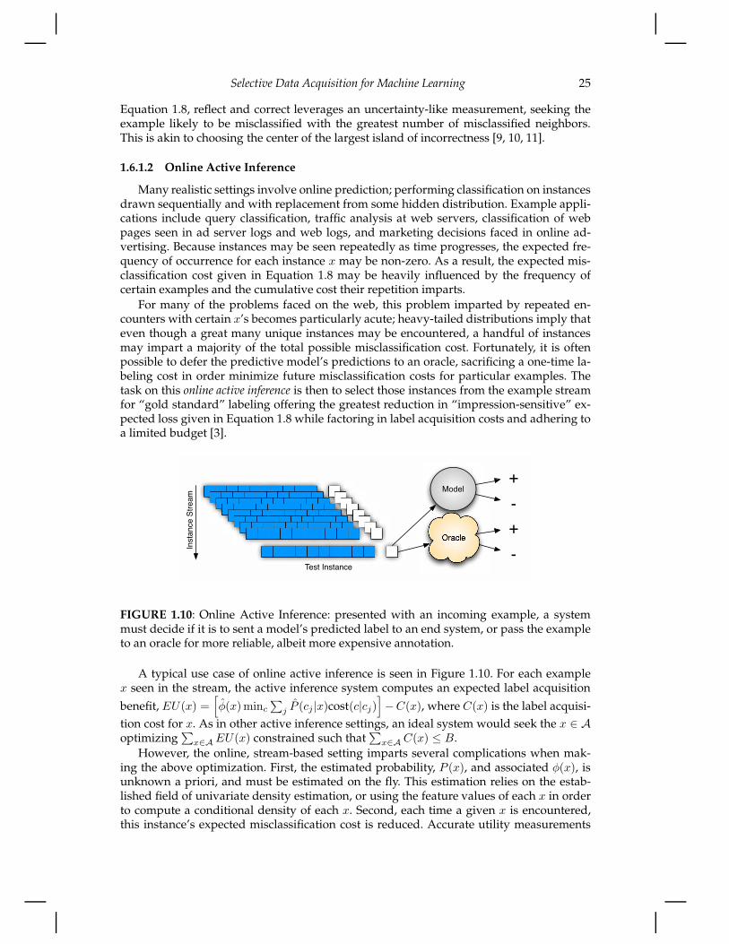
1.6.1.2 Online Active Inference
Many realistic settings involve online prediction; performing classification on instancesdrawn sequentially and with replacement from some hidden distribution. Example appli-cations include query classification, traffic analysis at web servers, classification of webpages seen in ad server logs and web logs, and marketing decisions faced in online ad-vertising. Because instances may be seen repeatedly as time progresses, the expected fre-quency of occurrence for each instance x may be non-zero. As a result, the expected mis-classification cost given in Equation 1.8 may be heavily influenced by the frequency ofcertain examples and the cumulative cost their repetition imparts.
For many of the problems faced on the web, this problem imparted by repeated en-counters with certain x’s becomes particularly acute; heavy-tailed distributions imply thateven though a great many unique instances may be encountered, a handful of instancesmay impart a majority of the total possible misclassification cost. Fortunately, it is oftenpossible to defer the predictive model’s predictions to an oracle, sacrificing a one-time la-beling cost in order minimize future misclassification costs for particular examples. Thetask on this online active inference is then to select those instances from the example streamfor “gold standard” labeling offering the greatest reduction in “impression-sensitive” ex-pected loss given in Equation 1.8 while factoring in label acquisition costs and adhering toa limited budget [3].
Instance Stream
Oracle
Model
Test Instance
+
-
+
-
FIGURE 1.10: Online Active Inference: presented with an incoming example, a systemmust decide if it is to sent a model’s predicted label to an end system, or pass the exampleto an oracle for more reliable, albeit more expensive annotation.
A typical use case of online active inference is seen in Figure 1.10. For each examplex seen in the stream, the active inference system computes an expected label acquisition
benefit, EU(x) =[
φ(x)minc
∑
j P (cj |x)cost(c|cj)]
−C(x), where C(x) is the label acquisi-
tion cost for x. As in other active inference settings, an ideal system would seek the x ∈ Aoptimizing
∑
x∈A EU(x) constrained such that∑
x∈A C(x) ≤ B.
However, the online, stream-based setting imparts several complications when mak-ing the above optimization. First, the estimated probability, P (x), and associated φ(x), isunknown a priori, and must be estimated on the fly. This estimation relies on the estab-lished field of univariate density estimation, or using the feature values of each x in orderto compute a conditional density of each x. Second, each time a given x is encountered,this instance’s expected misclassification cost is reduced. Accurate utility measurements

26 Cost-sensitive Learning
require that this reduction in expected cost should be extrapolated to the future. A thirdcomplication stems from how the budget, B is set. A budget-per-instance a one-time fixedbudget, and periodic fixed budgets yield different objective functions, complicating thetask faced in online active inference.
A fourth and particularly insidious difficultly stems from the fact that P (x) is unknown.This implies that a system sampling a stream of examples from P (x) may not even knowthe set of unique x’s that can potentially be encountered; as a consequence, the set of util-ities under consideration. However, it is possible to build a distribution on the expectedutility values conditioned on the probability of at least one occurrence during the timeperiod under consideration. An appropriate lower bound, τ can then be chosen wherebylabeling all examples with a utility greater than τ gathers as many of the highest utilityexamples as is possible while exhausting the available budget during that time period [3].
While labeling for the purpose of online active inference, it is also appealing to considerhow these labeled examples reduce overall cost via incorporation into the training set andupdating the underlaying model. Indeed, it is reasonable to consider how to allocate a sin-gle budget in order to achieve the best overall performance, while taking into account bothactive learning and active inference. While it is an interesting direction to consider how ex-pected utility-optimizing techniques for active learning can be incorporated into the samescale as the proposed technique for online active inference, it can be shown that by thoseexamples with the hightest EU(x) for active inference doubles as a generalized uncertaintysampling strategy for active learning potentially offering reasonable label choices for thetask of model improvement while explicitly reducing misclassification cost [3].
1.6.2 Prediction Time Active Feature Value Acquisition
In many domains we can acquire additional information for selected test instances thatmay help improve our classification performance on the test set. When this additional in-formation comes at a cost, or is potentially noisy, it is best to actively select the instancesthat are most likely to benefit from acquiring additional information. This problem ofprediction-time Active Feature-value Acquisition is analogous to AFA during inductionas discussed in Section 1.3. This setting has been studied in the context of customer tar-geting models [37], where, when making a decision for a customer, additional informationmay be purchased, if necessary, to make a more informed decision.
At the time of classifier induction, class labels are available for all instances includingthe incomplete instances. This information can be used effectively to estimate the poten-tial value of acquiring more information for the incomplete instances. However, this labelinformation is obviously not present during prediction on test instances. Yet, we must eval-uate the benefit of acquiring additional features for an incomplete instance, versus makinga prediction using only incomplete feature information.
However, uncertainty-based heuristics are still applicable in this setting. In particular,given a set of incomplete test instances, one can apply a previously-trained classifier to pre-dict the class membership probabilities of these instances, using only the feature-valuesthat are known. The uncertainty of these predictions can be computed using a measuresuch as unlabeled margin in Equation 1.2. Then all the feature-values for the most uncer-tain instances can be acquired until the acquisition budget is exhausted.
The above Uncertainty Sampling strategy aims to obtain more information about anuncertain prediction, with the hope that it will allow a more certain prediction, which inturn is assumed to result in a more accurate prediction. Even if more certain predictions arelikely to be more accurate, acquiring additional information on the most uncertain instancemay not result in the highest payoff. For example, if an instance is inherently ambiguous.Alternatively, we can select additional features-values only if they are expected to reduce
Selective Data Acquisition for Machine Learning 27
the uncertainty in classification after acquisition. Again, this can be viewed as a specialcase of the Expected Utility framework, where utility U in Equation 1.4 can be measuredby the log of the unlabeled margin [37].
Another factor to be taken into consideration at prediction-time is the cost of misclas-sifying an instance. Often misclassification costs are non-symmetric, such as the cost ofmisclassifying a malignant tumor as being benign. In such cases, one needs to weigh thecost of acquisitions with the cost of misclassification for each test instance. When acqui-sition and misclassification costs can be represented in the same units, we can selectivelyacquire feature values, so as to minimize the sum of the acquisition cost and expectedmisclassification cost [81].
Just as misclassification costs associated with different types of errors may not be uni-form, it is also often possible to acquire arbitrary subsets of feature values, each at a dif-ferent cost, a setting that has not been extensively explored in the research literature. Itmay be natural to extend the Expected Utility framework to consider sets of categoricalfeatures. However, estimating the joint probability distribution of all possible sets of val-ues may render such a policy hopelessly inefficient. To overcome the constraints of thiscomputational complexity, one may consider only potentially relevant feature subsets foracquisition, by combining innovative data structures and dynamic programming for incre-mentally updating the search space of informative subsets as new evidence is acquired—exploiting dependencies between missing features so as to share information value com-putations between different feature subsets, making the computation of the informationvalue of different feature subsets tractable [8].
Finally, if we know that feature values can be acquired at test time, it would make senseto account for this at the time of classifier induction. For example, by avoiding expensivefeatures at induction that may result in a more accurate model, but are not worth the cost atprediction time. Such a setting can be addressed in a budgeted learning framework wherea learner can spend a fixed learning budget bl to acquire training data, so as to produce aclassifier that spends at most bc per test instance[38].
1.7 Alternative acquisition settings
There are other sorts of data that can be acquired at a cost to improve machine learn-ing, besides the values for individual variables for the construction of predictive models.This section covers some alternative settings for applying a modeling budget. This sectionbegins with a treatment of the active collection of feature values for the purpose of per-forming unsupervised learning. Here, additional information may be acquired in order toimprove the quality of tasks such as clustering.
This section then continues to investigate the selection of entire examples by class, inorder that the training data comprise a “better” proportion of the constituent classes. Wethen discuss the related scenario where a human can be deployed to search for relevantinformation, for example, instances belonging to a given class, as well as feature valuesand feature labels. Finally, we present the important and often-ignored fact that in manypractical situations, learned models are applied in a decision-making context, where max-imizing the accuracy (or some other decision-agnostic measure) of one model is not theultimate goal. Rather, we want to optimize decision making. Decision-focused strategiesmay acquire different data from model-focused strategies.
28 Cost-sensitive Learning
1.7.1 Information Acquisition for Unsupervised Learning
Almost all work in information acquisition has addressed supervised settings. How-ever information may also be acquired for unstructured tasks, such as clustering. Inter-estingly, different clustering approaches may employ different types of information whichmay be potentially acquired at a cost, such as constraints as well as feature values.
Most clustering policies assume that each instance is represented by a vector of featurevalues. As is the case in supervised learning, clustering is undermined when the instancerepresentation is incomplete and can therefore benefit from effective policies to improveclustering through cost-effective acquisition of information. Consider for example data onconsumers’ preferences. Clustering can be applied to this data in order to derive naturalgroupings of products based on customer preferences, such as for data-driven discoveryof movie genres [6]. Clustering has also been used to help produce product/service rec-ommendations to consumers [30]. In all these cases, performance can be improved withcost-effective acquisition of information.
Let us first consider the Expected Utility framework for clustering. On the outset it mayappear that, given clustering algorithms typically aim to optimize some objective function,changes in the value of this function can be used to reflect the utility U from prospectivefeature value acquisitions. However, recall that typically only different clustering assign-ments yield changes in the corresponding clustering algorithm’s objective function. Yet, asnoted in [91], a costly feature value acquisition may alter the value of algorithm’s objec-tive function, without changing the assignment of even a single instance into a differentcluster. For the popular K-means clustering algorithm, for example, such an approach mayselect feature values that alter cluster centroid locations (decreasing the total distances be-tween instances and their respective centroids); however, these changes may not changethe cluster assignments significantly or at all. The effect of such wasteful acquisitions canbe significant. Alternatively, it is useful to consider utilities which capture the impact onclustering configuration caused by an acquisition. For example, utility can be measured bythe number of instances for which cluster membership changes as the result of an acquisi-tion [91].
Some clustering approaches do not employ a vectorial data representation; instead,the proximity of pairs of instances is provided. Hence, for a data set with N instances,the required information scales with O(N2). It has been shown [34, 15] that identifyingthe most informative proximity measures to acquire can be critical for overcoming the in-herent data sparseness of proximity data, making such methods feasible in practice. Forexample, using the expected value of information to quantify the gain from additional in-formation, [34] proposed an algorithm which identifies proximity values so as to minimizethe risk from estimating clusters from the existing data. Thus, selected acquisitions aim tominimize the loss from deciding only based on the incomplete information instead of theoptimal decision, when all proximity values are known.
Semi supervised clustering also offers interesting opportunities to acquire limited su-pervision to improve clustering cost-effectively. For example, a subset of instances, must-link and cannot-link constraints can specify instance pairs that must and must-not belongto the same cluster, respectively. Similarly, cluster-level constraints indicate whether ornot instances in two different clusters ought to be assigned to the same cluster. To im-prove clustering, an information acquisition policy may suggest the constraints for whichpairs would be most informative to acquire. Similar to active learning, the feature values,from which distances are derived, are known. Acquiring constraints for clustering may

Selective Data Acquisition for Machine Learning 29
not bear much similarity to instance-level information acquisition for supervised learning.However, the uncertainly reduction principle has been effectively adapted to this settingas well. Specifically, for cluster-level constraint acquisition [39] proposes to acquire con-straints when it is most difficult to determine whether two clusters should be merged.In contrast, for acquiring instance-level constraints, [7] proposes a policy which doesnot follow principles used in supervised settings. In particular, given the impact of ini-tial centroids on clustering outcomes of the K-means clustering algorithm, they proposea constraint acquisition policy which improves the identification of cluster centroids andtheir neighborhoods with fewer queries. To accomplish this, they employ the farthest firsttraversal scheme to identify points from different clusters using fewer queries. A subse-quent consolidation phase, acquires additional pair-wise constraints to explore the struc-ture of each cluster’s neighborhood.
In future work it would be interesting to consider policies that can consider differenttypes of information, such as constraints information and feature values, which may beacquired at different costs. However, as reflected in the work we discuss above, and quitedifferently from the supervised setting, employing the Expected Utility framework for thistask may not be the obvious choice in this case.
1.7.2 Class-Conditional Example Acquisition
In many model induction tasks, the amount of training data is constrained not by thecost of instance labels, but by the cost of gathering the independent covariates that areused to predict these labels. For example, in certain settings examples can be acquired byclass, but gathering the feature values requires costly physical tests and experiments, largeamounts of time or computation, or some other source of information that requires somebudget outlay. Consider, for example, the problem of building predictive models based ondata collected through an “artificial nose” with the intent of “sniffing out” explosive orhazardous chemical compounds [48, 50, 49]. In this setting, the reactivity of a large num-ber of chemicals are already known, representing label-conditioned pools of available in-stances. However, producing these chemicals in a laboratory setting and running the resul-tant compound through the artificial nose may be an expensive, time-consuming process.This problem appears to face the inverse of the difficulties faced by active learning—labelsessentially come for free, while the independent feature values are completely unknownand must be gathered at a cost (let’s say, all at once). In this setting, it becomes importantto consider the question: “in what proportion should classes be represented in a trainingset of a certain size?” [95]
Let’s call the problem of proportioning class labels in a selection of n additional train-ing instances, ”Active Class Selection” (ACS) [48, 50, 49, 95]. This process is exemplified inFigure 1.11. In this setting, there is assumed to be large, class-conditioned (virtual) poolsof available instances with completely hidden feature values. At each epoch, t, of the ACSprocess, the task is to leverage the current model when selecting examples from these poolsin a proportion believed to have the greatest effectiveness for improving the generalizationperformance of this model. The feature values for each instance are then collected and thecomplete instances are added to the training set. The model is re-constructed and the pro-cesses is repeated until n examples are obtained (because the budget is exhausted or someother stopping criterion is met, such as a computational limit). Note that this situation canbe considered to be a special case of the instance completion setting of Active Feature Ac-quisition (discussed above). It is a degenerate special case because, prior to selection, thereis no information at all about the instances other than their classes.
For ACS, the extreme lack of information to guide selection leads to the developmentof unique uncertainty and utility estimators, which, in the absence of predictive covariates,
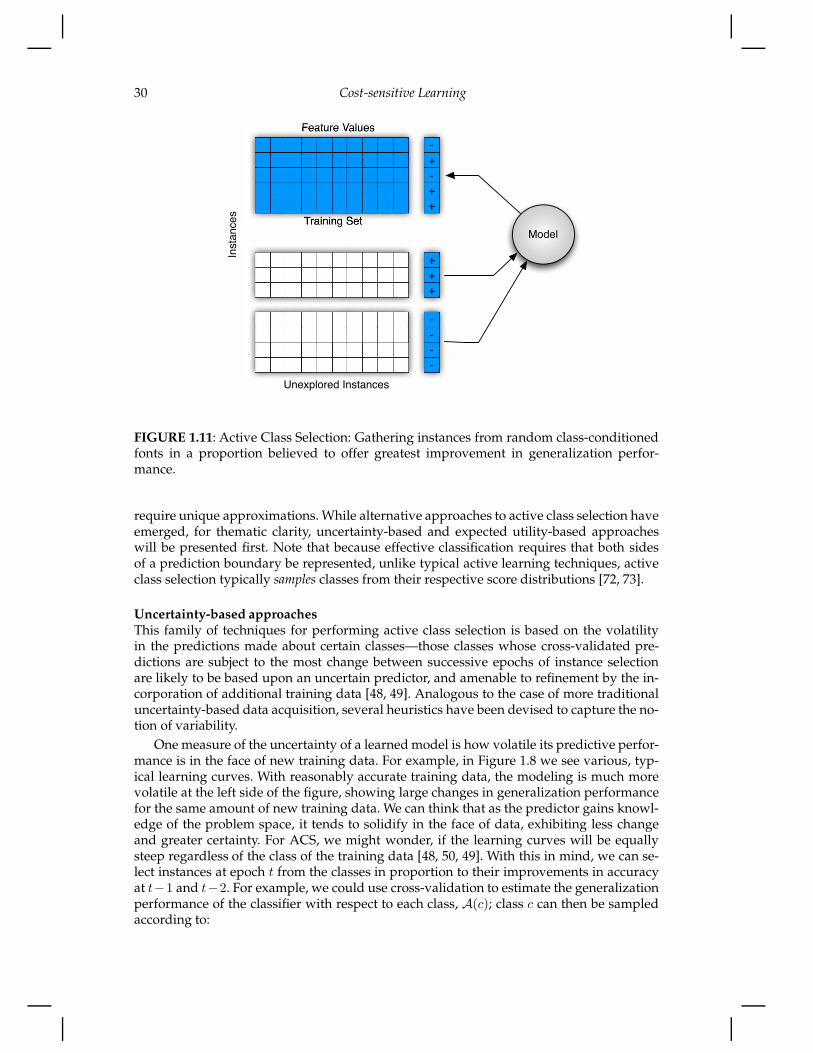
30 Cost-sensitive Learning
+
+
-
+
-
Instances
Feature Values
+
+
+
-
-
-
-
Training Set
Model
Unexplored Instances
FIGURE 1.11: Active Class Selection: Gathering instances from random class-conditionedfonts in a proportion believed to offer greatest improvement in generalization perfor-mance.
require unique approximations. While alternative approaches to active class selection haveemerged, for thematic clarity, uncertainty-based and expected utility-based approacheswill be presented first. Note that because effective classification requires that both sidesof a prediction boundary be represented, unlike typical active learning techniques, activeclass selection typically samples classes from their respective score distributions [72, 73].
Uncertainty-based approachesThis family of techniques for performing active class selection is based on the volatilityin the predictions made about certain classes—those classes whose cross-validated pre-dictions are subject to the most change between successive epochs of instance selectionare likely to be based upon an uncertain predictor, and amenable to refinement by the in-corporation of additional training data [48, 49]. Analogous to the case of more traditionaluncertainty-based data acquisition, several heuristics have been devised to capture the no-tion of variability.
One measure of the uncertainty of a learned model is how volatile its predictive perfor-mance is in the face of new training data. For example, in Figure 1.8 we see various, typ-ical learning curves. With reasonably accurate training data, the modeling is much morevolatile at the left side of the figure, showing large changes in generalization performancefor the same amount of new training data. We can think that as the predictor gains knowl-edge of the problem space, it tends to solidify in the face of data, exhibiting less changeand greater certainty. For ACS, we might wonder, if the learning curves will be equallysteep regardless of the class of the training data [48, 50, 49]. With this in mind, we can se-lect instances at epoch t from the classes in proportion to their improvements in accuracyat t−1 and t−2. For example, we could use cross-validation to estimate the generalizationperformance of the classifier with respect to each class, A(c); class c can then be sampledaccording to:

Selective Data Acquisition for Machine Learning 31
ptA(c) ∝
max{
0,At−1(c) −At−2(c)}
∑
c′ max {0,At−1(c′) −At−2(c′)}
Alternatively, we could consider general volatility in class members’ predicted labels,beyond improvement in the model’s ability to predict the class. Again, by using cross-validated predictions at successive epochs, it is possible to isolate members of each class,and observe changes in the predicted class for each instance. For example, when the pre-dicted label of a given instance changes between successive epochs, we can deem the in-stance to have been redistricted [48, 50, 49]. Again considering the level of volatility in amodel’s predictions to be a measurement of uncertainty, we can sample classes at epoch t
according to each classes’ proportional measure of redistricting:
ptR(c) ∝
1|c|
∑
x∈c I(f t−1(x) 6= f t−2(x))∑
c′1
|c′|
∑
x∈c′ I(f t−1(x) 6= f t−2(x))
Where I(·) is an indicator function taking the value of 1 if its argument is true and 0 oth-erwise. f t−1(x) and f t−2(x) are the predicted labels for instance x from the models trainedat epoch t − 1 and t − 2 respectively [48, 50, 49].
Expected Class UtilityThe previously described active class selection heuristics are reliant on the assumptionthat adding examples belonging to a particular class will improve the predictive accuracywith respect to that class. This does not directly estimate the utility of adding members ofa particular class to a model’s overall performance. Instead, it may be preferable to selectclasses whose instances’ presence in the training set will reduce a model’s misclassificationcost by the greatest amount in expectation.
Let cost(ci|cj) be the cost of predicting ci on an instance x whose true label is cj . Thenthe expected empirical misclassification cost over a sample data set, D is:
R =1
|D|
∑
x∈D
∑
i
P (ci|x)cost(ci|y)
Where y is the correct class for a given x. Typically in the active class selection set-ting, this expectation would be taken over the training set (e.g. D = T ), preferably usingcross-validation. In order to reduce this risk, we would like to select examples from class c
leading to the greatest reduction in this expected risk [50].
Consider a predictive model PT∪c(·|x), a model built on the training set, T , supple-mented with an arbitrary example belonging to class c. Given the opportunity to choosean additional class-representative example to the training pool, we would like to select theclass that reduces expected risk by the greatest amount:
c = argmaxc
U(c)
Where
U(c) =1
|D|
∑
x∈D
∑
i
PT (ci|x)cost(ci|y) −1
|D|
∑
x∈D
∑
i
PT∪c(ci|x)cost(ci|y)
Of course the benefit of adding additional examples on a test data set is unknown.Furthermore, the impact of a particular class’s examples may vary depending on the fea-ture values of particular instances. In order to cope with these issues, we can estimate viacross-validation on the training set. Using sampling, we can try various class-conditional
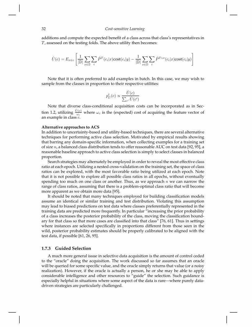
32 Cost-sensitive Learning
additions and compute the expected benefit of a class across that class’s representatives inT , assessed on the testing folds. The above utility then becomes:
U(c) = Ex∈c
[
1
|D|
∑
x∈D
∑
i
PT (ci|x)cost(ci|y) −1
|D|
∑
x∈D
∑
i
PT∪c(ci|x)cost(ci|y)
]
Note that it is often preferred to add examples in batch. In this case, we may wish tosample from the classes in proportion to their respective utilities:
pt
U(c) ∝
U(c)∑
c′ U(c′)
Note that diverse class-conditional acquisition costs can be incorporated as in Sec-
tion 1.2, utilizing U(c)ωc
where ωc is the (expected) cost of acquiring the feature vector ofan example in class c.
Alternative approaches to ACSIn addition to uncertainty-based and utility-based techniques, there are several alternativetechniques for performing active class selection. Motivated by empirical results showingthat barring any domain-specific information, when collecting examples for a training setof size n, a balanced class distribution tends to offer reasonable AUC on test data [92, 95], areasonable baseline approach to active class selection is simply to select classes in balancedproportion.
Search strategies may alternately be employed in order to reveal the most effective classratio at each epoch. Utilizing a nested cross-validation on the training set, the space of classratios can be explored, with the most favorable ratio being utilized at each epoch. Notethat it is not possible to explore all possible class ratios in all epochs, without eventuallyspending too much on one class or another. Thus, as we approach n we can narrow therange of class ratios, assuming that there is a problem-optimal class ratio that will becomemore apparent as we obtain more data [95].
It should be noted that many techniques employed for building classification modelsassume an identical or similar training and test distribution. Violating this assumptionmay lead to biased predictions on test data where classes preferentially represented in thetraining data are predicted more frequently. In particular ”increasing the prior probabilityof a class increases the posterior probability of the class, moving the classification bound-ary for that class so that more cases are classified into that class” [76, 61]. Thus in settingswhere instances are selected specifically in proportions different from those seen in thewild, posterior probability estimates should be properly calibrated to be aligned with thetest data, if possible [61, 26, 95].
1.7.3 Guided Selection
A much more general issue in selective data acquisition is the amount of control cededto the “oracle” doing the acquisition. The work discussed so far assumes that an oraclewill be queried for some specific value, and the oracle simply returns that value (or a noisyrealization). However, if the oracle is actually a person, he or she may be able to applyconsiderable intelligence and other resources to “guide” the selection. Such guidance isespecially helpful in situations where some aspect of the data is rare—where purely data-driven strategies are particularly challenged.

Selective Data Acquisition for Machine Learning 33
Let’s continue thinking about the active class selection setting as a concrete case. Inmany practical settings, one class is quite rare. As a motivational example, consider build-ing a predictive model from scratch designed to classify web pages containing a particulartopic of interest. While large absolute numbers of such web pages may be present on theweb, they may be outnumbered by uninteresting pages by a million to one or worse (take,for instance, the task of detecting and removing hate speech from the web [5]).
Unfortunately, when the class distribution is so skewed, active learning strategies canfail completely—and the failure is not simply due to the hurdles faced when trying to learnmodels in settings with skewed class distribution, a problem that has received a fair bit ofattention [93, 4]. Rather, the problem faced by the active learner is far more treacherous:learning techniques cannot even concentrate on the rare instances as the techniques areunaware which instances to focus on.
Perhaps even more insidious is the difficulty posed by classes consisting of rare, dis-junctive sub-concepts. These disjuncts can emerge even in problems spaces without suchan extreme class skew: when members of an important class do not manifest themselves asa simple, continuously dense region of the input space, but rather as many small disjointclusters embedded throughout the input space [94]. For an active learner, these “small dis-juncts” act like rare classes: when an active learner has not been exposed to instances of asub-concept, how can it best choose instances to label in order to properly distinguish thatsubconcept from its containing space?
While a plethora of techniques have been proposed for performing active learningspecifically in the high-skew setting [89, 13, 104, 27] as well as techniques where the geome-try and feature-density of the problem space are explicitly included when making instanceselections [105, 33, 21, 59, 98, 53], these techniques, as initially appealing as they may seem,may fail just as badly as traditional active learning techniques. Class skew and sub-conceptrarity may be sufficient to thwart them completely [5, 4].
However, in these extremely difficult settings, we can task humans to search the prob-lem space for rare cases, using tools (like search engines) and possibly interacting withthe base learner. Consider the motivating example of hate speech classification on the web(from above). While an active learner may experience difficulty exploring the details ofthis rare class, a human oracle armed with a search interface is likely to expose examplesof hate speech easily. In fact, given the coverage of modern web search engines, a humancan produce interesting examples from a much larger sample of the problem space, farbeyond that which is likely to be contained in a sample pool for active learning. This iscritical due to hardware-imposed constraints on the size of the pool an active learner isable to choose from—e.g., a random draw of several hundred thousand examples fromthe problem space may not even contain any members of the minority class or of raredisjuncts!
Guided Learning is the general process of utilizing oracles to search the problem space,using their domain expertise to seek instances representing the interesting regions of theproblem space. Figure 1.12 presents the general guided learning setting. Here, given someinterface enabling search over the domain in question, an oracle searches for interestingexamples, which are either supplemented with an implicit label by the oracle, or sent forexplicit labeling as a second step. These examples are then added to the training set and amodel is re-trained. Oracles can leverage their background knowledge of the problem be-ing faced. By incorporating the techniques of active class selection oracles can be directedto gather instances in a class-proportion believed to most strongly help train a model. Fur-ther, by allowing the oracle to interact with the base learner, confusing instances, thosethat “fool” the model can be sought out from the problem space and used for subsequenttraining in a form of human-guided uncertainty sampling.
While guided learning often presents an attractive and cost-effective alternative to ac-
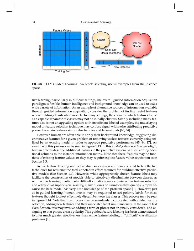
34 Cost-sensitive Learning
-
+
-
+
-
+
-
+
-
Instances
Feature Values
InstanceSpace
Oracle
New Instance
Training Set
Seek OutUseful Instances
FIGURE 1.12: Guided Learning: An oracle selecting useful examples from the instancespace.
tive learning, particularly in difficult settings, the overall guided information acquisitionparadigm is flexible, human intelligence and background knowledge can be used to seek awide variety of information. As an example of alternative sources of information availablethrough guided information acquisition, consider the problem of finding useful featureswhen building classification models. In many settings, the choice of which features to useas a capable separator of classes may not be initially obvious. Simply including many fea-tures also is not an appealing option; with insufficient labeled examples, the underlayingmodel or feature selection technique may confuse signal with noise, attributing predictivepower to certain features simply due to noise and false-signals [65, 64].
However, human are often able to apply their background knowledge, suggesting dis-criminative features for a given problem or removing useless features currently being uti-lized by an existing model in order to approve predictive performance [65, 64, 17]. Anexample of this process can be seen in Figure 1.13. In this guided feature selection paradigm,human oracles describe additional features to the predictive system, in effect adding addi-tional columns to the instance information matrix. Note that these features may be func-tions of existing feature values, or they may require explicit feature value acquisition as inSection 1.3.
Active feature labeling and active dual supervision are demonstrated to be effectivetechniques for reducing the total annotation effort required for building effective predic-tive models (See Section 1.4). However, while appropriately chosen feature labels mayfacilitate the construction of models able to effectively discriminate between classes, aswith active learning, particularly difficult situations may stymie active feature selectionand active dual supervision, wasting many queries on uninformative queries, simply be-cause the base model has very little knowledge of the problem space [1]. However, justas in guided learning, human oracles may be requested to seek polarity labels for thosefeatures thought to most effectively discern between the classes. This process may be seenin Figure 1.14. Note that this process may be seamlessly incorporated with guided featureselection, adding new features and their associated label simultaneously. In the case of textclassification, this may involve adding a term or phrase not originally considered, and as-signing to that phrase a class polarity. This guided feature labeling has been demonstratedto offer much greater effectiveness than active feature labeling in “difficult” classificationproblems [1].
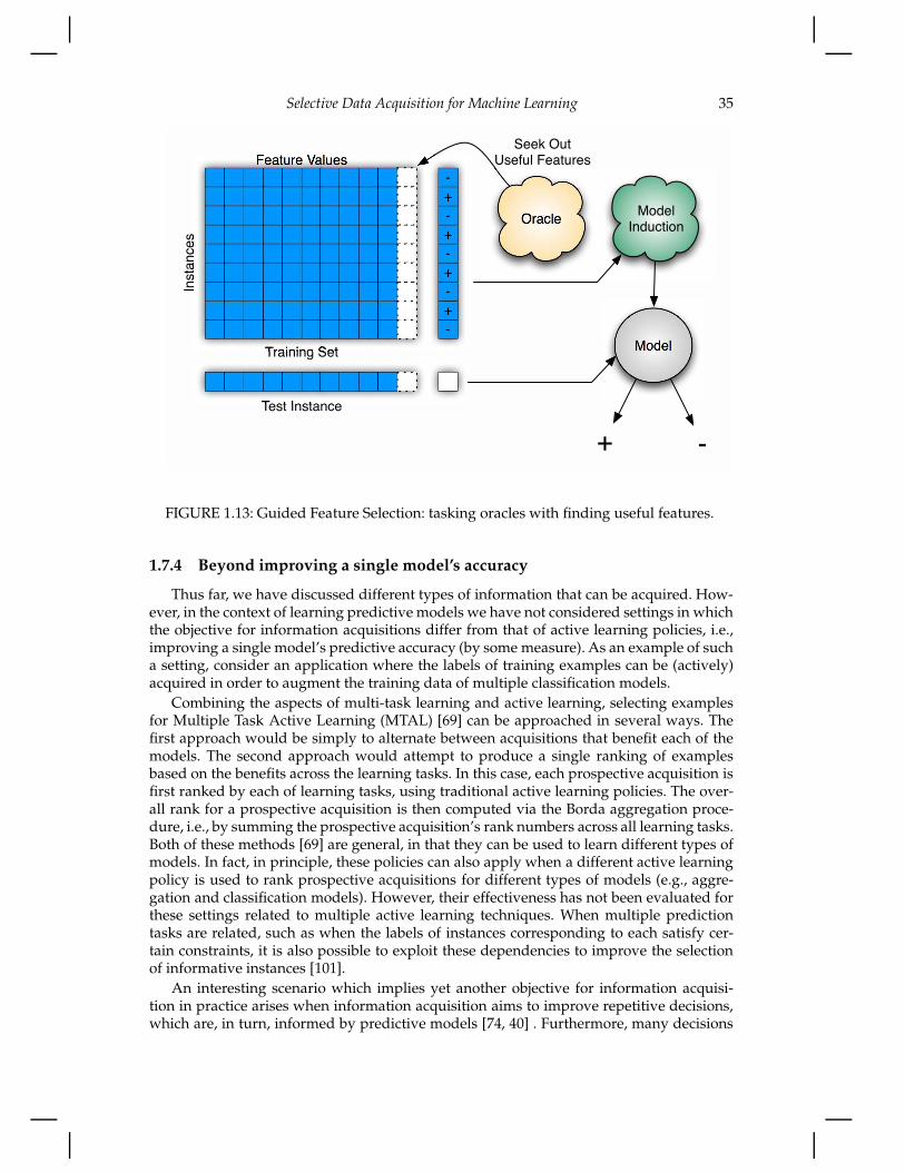
Selective Data Acquisition for Machine Learning 35
-
+
-
+
-
+
-
+
-Instances
Feature Values
Oracle
Training Set
Seek OutUseful Features
Test Instance
Model
Model Induction
+ -
FIGURE 1.13: Guided Feature Selection: tasking oracles with finding useful features.
1.7.4 Beyond improving a single model’s accuracy
Thus far, we have discussed different types of information that can be acquired. How-ever, in the context of learning predictive models we have not considered settings in whichthe objective for information acquisitions differ from that of active learning policies, i.e.,improving a single model’s predictive accuracy (by some measure). As an example of sucha setting, consider an application where the labels of training examples can be (actively)acquired in order to augment the training data of multiple classification models.
Combining the aspects of multi-task learning and active learning, selecting examplesfor Multiple Task Active Learning (MTAL) [69] can be approached in several ways. Thefirst approach would be simply to alternate between acquisitions that benefit each of themodels. The second approach would attempt to produce a single ranking of examplesbased on the benefits across the learning tasks. In this case, each prospective acquisition isfirst ranked by each of learning tasks, using traditional active learning policies. The over-all rank for a prospective acquisition is then computed via the Borda aggregation proce-dure, i.e., by summing the prospective acquisition’s rank numbers across all learning tasks.Both of these methods [69] are general, in that they can be used to learn different types ofmodels. In fact, in principle, these policies can also apply when a different active learningpolicy is used to rank prospective acquisitions for different types of models (e.g., aggre-gation and classification models). However, their effectiveness has not been evaluated forthese settings related to multiple active learning techniques. When multiple predictiontasks are related, such as when the labels of instances corresponding to each satisfy cer-tain constraints, it is also possible to exploit these dependencies to improve the selectionof informative instances [101].
An interesting scenario which implies yet another objective for information acquisi-tion in practice arises when information acquisition aims to improve repetitive decisions,which are, in turn, informed by predictive models [74, 40] . Furthermore, many decisions

36 Cost-sensitive Learning
-
+
+
-
+
+ - - + -Instances
Instance
Labels
Test Instance
Feature Labels
Dual-
Trained
Model
Model
Induction
+ -
Feature Values
Oracle
Seek Out
Discriminative
Feature Labels
FIGURE 1.14: Guided Feature Labeling: tasking oracles with finding features and theirassociated class polarity believed to be best able to discriminate between classes.
are informed by multiple predictive models of different types. For instance, firms’ salestax audit decisions are typically informed by the predicted probability of tax fraud, butalso by the predicted revenue that might be recovered. Note that prospective audit acqui-sitions will affect both predictive models. Interestingly, for each model, a different auditacquisition might be more desirable to improve the corresponding estimation. Hence, it isbeneficial to understand how should an acquisition budget be allocated among them so asto benefit future audit decisions the most?
In principle, MTAL can be applied to cost-effectively improve the predictive accuracyof all the models informing the decisions. However, costly improvements in model accu-racy does not necessarily yield better decisions [74]. Hence, more efficient policies can bederived if such greedy improvements in accuracy are avoided. Furthermore, exploitingknowledge of the decision’s structure can yield significant benefits [74, 40, 41]. For exam-ple, when information is acquired for multiple models informing the decisions, it is usefulto consider how changes in all of the models simultaneously will affect future decisions.This approach has been applied effectively when the same information can augment mul-tiple models simultaneously [40, 41]. It will also be useful to study the effectiveness ofthis general principle when the training data of each of the models can be augmented byacquisition from a different source (i.e., the same acquisition cannot be used to train allmodels).

Selective Data Acquisition for Machine Learning 37
1.8 Conclusion
The vast majority of the information acquisition literature focuses on active learning,reflecting only a single setting— the selection of individual instances for the acquisitionof a single, correct label with the objective of improving classification performance costeffectively. However, as we outline in this chapter, a rich set of important practical prob-lems arise once we consider the diverse set of information that is available to a machinelearning system at some cost, and when the error-free assumptions typically used in suchresearch are relaxed. In this chapter, we discussed three dimensions that define alternativeinformation acquisition problems. Specifically these facets are: the different types of infor-mation that can be acquired to inform learning, the quality of the acquired information,and the different objectives which acquisitions ultimately aim to improve, cost-effectively.Since each of these facets can take a variety of settings in practice, cost-effective informa-tion acquisition gives rise to a diverse range of important problems.
In order to cope with the complexity of such a diverse range of problems, we have pre-sented two general strategies for information acquisition. Namely, uncertainty reductionand expected utility approaches. While uncertainty-based approaches are appealing ini-tially in that they are often simple to implement and have been subject to extensive study inthe realm of traditional active learning, these techniques tend to fall short when faced withthe more complex demands of general information acquisition. Combining effectivenessmeasures for diverse types of information seamlessly in concert with acquisition costs isoften beyond the capability of uncertainty-based techniques. Fortunately, expected utility-based approaches offer a one-size-fits-all framework for integrating the empirical benefitsof different acquisition types with the costs these acquisitions may incur. While expectedutility approaches offer great promise, this is tempered by the difficulties associated withcomputing an accurate utility estimator in a way that is computationally tractable.
While we have demonstrated a wide range of use cases and settings for selective dataacquisition, discussing applications ranging from marketing to medicine, there are innu-merable scenarios yet to be explored; more complex combinations of data available at acost, both at training and at use time, with relaxed assumptions regarding data cleanliness.Though it’s difficult to speculate what new applications and future research into the realmof data acquisition will accomplish, we believe that the material presented here provides asolid foundation upon which this new work can build.

38 Cost-sensitive Learning

Bibliography
[1] Josh Attenberg, Prem Melville, and Foster Provost. Guided feature labeling forbudget-sensitive learning under extreme class imbalance. In BL-ICML ’10: Workshopon Budgeted Learning, 2010.
[2] Josh Attenberg, Prem Melville, and Foster J. Provost. A unified approach to activedual supervision for labeling features and examples. In ECML/PKDD, 2010.
[3] Josh Attenberg and Foster Provost. Active inference and learning for classifyingstreams. In BL-ICML ’10: Workshop on Budgeted Learning, 2010.
[4] Josh Attenberg and Foster Provost. Inactive learning? difficulties employing activelearning in practice. SIGKDD Explorations, 12(2), 2010.
[5] Josh Attenberg and Foster Provost. Why label when you can search? strategies forapplying human resources to build classification models under extreme class imbal-ance. In KDD, 2010.
[6] Arindam Banerjee, Chase Krumpelman, Sugato Basu, Raymond J. Mooney, and Joy-deep Ghosh. Model-based overlapping clustering. In Proc. of 11th ACM SIGKDDIntl. Conf. on Knowledge Discovery and Data Mining (KDD-05), 2005.
[7] Sugato Basu. Semi-supervised clustering with limited background knowledge. InAAAI, pages 979–980, 2004.
[8] Mustafa Bilgic and Lise Getoor. Voila: Efficient feature-value acquisition for classifi-cation. In Proceedings of the Twenty-Second Conference on Artificial Intelligence (AAAI),pages 1225–1230, 2007.
[9] Mustafa Bilgic and Lise Getoor. Effective label acquisition for collective classifica-tion. In Proceeding of the 14th ACM SIGKDD international conference on Knowledgediscovery and data mining, KDD ’08, pages 43–51. ACM, 2008.
[10] Mustafa Bilgic and Lise Getoor. Reflect and correct: A misclassification predictionapproach to active inference. ACM Trans. Knowl. Discov. Data, 3, December 2009.
[11] Mustafa Bilgic and Lise Getoor. Active Inference for Collective Classification. InAAAI, 2010.
[12] Catherine L. Blake and Christopher John Merz. UCI repository of machine learningdatabases. http://www.ics.uci.edu/˜mlearn/MLRepository.html, 1998.
[13] Michael Bloodgood and K. Vijay Shanker. Taking into account the differences be-tween actively and passively acquired data: the case of active learning with supportvector machines for imbalanced datasets. In NAACL, 2009.
[14] Carla E. Brodley and Mark A. Friedl. Identifying mislabeled training data. Journal ofArtificial Intelligence Research, 11:131–167, 1999.
39
40 Cost-sensitive Learning
[15] Joachim M. Buhmann and Thomas Zoller. Active learning for hierarchical pairwisedata clustering. In ICPR, pages 2186–2189, 2000.
[16] Bob Carpenter. Multilevel bayesian model of categorical data annotation, 2008.Available at: http://lingpipe-blog.com/lingpipe-white-papers/.
[17] Bruce Croft and Raj Das. Experiments with query acquisition and use in documentretrieval systems. In In Proceedings of the ACM SIGIR Conference on Research and De-velopment in Information Retrieval, pages 349–368, 1990.
[18] B.V. Dasarathy, editor. Information Fusion:An International Journal on Multi-Sensor,Multi-Source Information Fusion. Elsevier, 2010.
[19] Alexander Philip Dawid and Allan M. Skene. Maximum likelihood estimation of ob-server error-rates using the EM algorithm. Applied Statistics, 28(1):20–28, September1979.
[20] O. Dekel and O. Shamir. Vox populi: Collecting high-quality labels from a crowd.In COLT 2009: Proceedings of the 22nd Annual Conference on Learning Theory. Citeseer,2009.
[21] P. Donmez and J. Carbonell. Paired Sampling in Density-Sensitive Active Learning.In Proc. 10 th International Symposium on Artificial Intelligence and Mathematics, 2008.
[22] Pinar Donmez and Jaime G. Carbonell. Proactive learning: Cost-sensitive activelearning with multiple imperfect oracles. In Proceedings of the 17th ACM Conferenceon Information and Knowledge Management (CIKM 2008), pages 619–628, 2008.
[23] Pinar Donmez, Jaime G. Carbonell, and Jeff Schneider. Efficiently learning the ac-curacy of labeling sources for selective sampling. In Proceedings of the 15th ACMSIGKDD International Conference on Knowledge Discovery and Data Mining (KDD 2009),pages 259–268, 2009.
[24] G. Druck, G. Mann, and A. McCallum. Learning from labeled features using gener-alized expectation criteria. In SIGIR, 2008.
[25] G. Druck, B. Settles, and A. McCallum. Active learning by labeling features. InEMNLP ’09, pages 81–90. Association for Computational Linguistics, 2009.
[26] Charles Elkan. The foundations of cost-sensitive learning. In In Proceedings of theSeventeenth International Joint Conference on Artificial Intelligence, pages 973–978, 2001.
[27] Seyda Ertekin, Jian Huang, Leon Bottou, and Lee Giles. Learning on the border:active learning in imbalanced data classification. In CIKM, 2007.
[28] Jerome H. Friedman, Ron Kohavi, and Yeogirl Yun. Lazy decision trees. InAAAI/IAAI, Vol. 1, pages 717–724, 1996.
[29] G. M. Fung, O. L. Mangasarian, and J. W. Shavlik. Knowledge-based support vec-tor machine classifiers. In Advances in Neural Information Processing Systems 14. MITPress, 2002.
[30] Thomas George and Srujana Merugu. A scalable collaborative filtering frameworkbased on co-clustering. In ICDM, pages 625–628, 2005.
[31] S. Godbole, A. Harpale, S. Sarawagi, and S. Chakrabarti. Document classificationthrough interactive supervision of document and term labels. In PKDD, 2004.

Selective Data Acquisition for Machine Learning 41
[32] R. Haertel, K. Seppi, E. Ringger, and J. Carroll. Return on investment for activelearning. In Proceedings of the NIPS Workshop on Cost-Sensitive Learning, 2008.
[33] Jingrui He and Jaime G. Carbonell. Nearest-neighbor-based active learning for rarecategory detection. In NIPS, 2007.
[34] Thomas Hofmann and Joachim M. Buhmann. Active data clustering. In Proceedingsof the 1997 conference on Advances in neural information processing systems 10, NIPS ’97,pages 528–534, Cambridge, MA, USA, 1998. MIT Press.
[35] P. Ipeirotis, F. Provost, V. Sheng, and J. Wang. Repeated labeling using multiple,noisy labelers. Technical Report Working Paper CeDER-10-03, Center for DigitalEconomy Research, NYU Stern School of Business, 2010.
[36] P.G. Ipeirotis, F. Provost, and J. Wang. Quality management on amazon mechanicalturk. In Proceedings of the ACM SIGKDD Workshop on Human Computation, pages64–67. ACM, 2010.
[37] Pallika Kanani and Prem Melville. Prediction-time active feature-value acquisitionfor customer targeting. In Proceedings of the Workshop on Cost Sensitive Learning, NIPS2008, 2008.
[38] Aloak Kapoor and Russell Greiner. Learning and classifying under hard budgets. InECML, pages 170–181, 2005.
[39] Dan Klein, Sepandar D. Kamvar, and Christopher D. Manning. From instance-levelconstraints to space-level constraints: Making the most of prior knowledge in dataclustering. In ICML, pages 307–314, 2002.
[40] Danxia Kong and Maytal Saar-Tsechansky. Collaborative information acquisition.In BL-ICML ’10: Workshop on Budgeted Learning, 2010.
[41] Danxia Kong and Maytal Saar-Tsechansky. A framework for collaborative informa-tion acquisition. In Workshop on Information Technology and Systems, 2010.
[42] Gautam Kunapuli, Kristin P. Bennett, Amina Shabbeer, Richard Maclin, and Jude W.Shavlik. Online knowledge-based support vector machines. In ECML/PKDD, pages145–161, 2010.
[43] Ludmila I. Kuncheva, Christopher J. Whitaker, Catherine A. Shipp, and Robert P.W.Duin. Limits on the majority vote accuracy in classifier fusion. Pattern Analysis andApplications, 6(1):22–31, April 2003.
[44] David Lewis and William Gale. A sequential algorithm for training text classifiers. InProc. of 17th Intl. ACM SIGIR Conf. on Research and Development in Information Retrieval(SIGIR-94), 1994.
[45] R. Little and D. Rubin. Statistical Analysis with Missing Data. John Wiley and Sons,,1987.
[46] Bing Liu, Xiaoli Li, Wee Sun Lee, and Philip Yu. Text classification by labeling words.In AAAI, 2004.
[47] Dan Lizotte, Omid Madani, and Russell Greiner. Budgeted learning of naive-Bayesclassifiers. In UAI, 2003.

42 Cost-sensitive Learning
[48] R. Lomasky, C. Brodley, M. Aernecke, D. Walt, and M. Friedl. Active Class Selection.In Machine Learning: ECML, volume 4701, pages 640–647, 2007.
[49] R. Lomasky, C. E. Brodley, S. Bencic, M. Aernecke, and D Walt. Guiding class se-lection for an artificial nose. In NIPS Workshop on Testing of Deployable Learning andDecision Systems, 2006.
[50] Rachel Lomasky. Active Acquisition of Informative Training Data. PhD thesis, TuftsUniversity, 2010.
[51] Gabor Lugosi. Learning with an unreliable teacher. Pattern Recognition, 25(1):79–87,January 1992.
[52] Andrew McCallum and Kamal Nigam. A comparison of event models for naiveBayes text classification. In AAAI Workshop on Text Categorization, 1998.
[53] Andrew K. Mccallum and Kamal Nigam. Employing em in pool-based active learn-ing for text classification. In ICML, 1998.
[54] Prem Melville, Wojciech Gryc, and Richard Lawrence. Sentiment analysis of blogsby combining lexical knowledge with text classification. In KDD, 2009.
[55] Prem Melville and Raymond J. Mooney. Diverse ensembles for active learning. InProc. of 21st Intl. Conf. on Machine Learning (ICML-2004), 2004.
[56] Prem Melville, Foster J. Provost, and Raymond J. Mooney. An expected utility ap-proach to active feature-value acquisition. In Proc. of 5th IEEE Intl. Conf. on DataMining (ICDM-05), pages 745–748, 2005.
[57] Prem Melville, Maytal Saar-Tsechansky, Foster J. Provost, and Raymond J. Mooney.Active feature-value acquisition for classifier induction. In Proc. of 4th IEEE Intl. Conf.on Data Mining (ICDM-04), pages 483–486, 2004.
[58] Prem Melville and Vikas Sindhwani. Active dual supervision: Reducing the cost ofannotating examples and features. In NAACL HLT 2009, 2009.
[59] Hieu T. Nguyen and Arnold Smeulders. Active learning using pre-clustering. InICML, 2004.
[60] Bo Pang, Lillian Lee, and Shivakumar Vaithyanathan. Thumbs up?: sentiment classi-fication using machine learning techniques. In Proceedings of the ACL-02 conference onEmpirical methods in natural language processing - Volume 10, EMNLP ’02, pages 79–86.Association for Computational Linguistics, 2002.
[61] F. Provost. Machine learning from imbalanced data sets 101. In Proceedings of theAAAI2000 Workshop on Imbalanced Data Sets, 2000.
[62] Foster Provost and Andrea Pohoreckyj Danyluk. Learning from bad data. In Pro-ceedings of the ML-95 Workshop on Applying Machine Learning in Practice, 1995.
[63] John Ross Quinlan. C4.5: Programs for Machine Learning. Morgan Kaufmann Publish-ers, Inc., 1992.
[64] Hema Raghavan, Omid Madani, and Rosie Jones. InterActive feature selection. InProceedings of the 19th international joint conference on Artificial intelligence, pages 841–846, 2005.

Selective Data Acquisition for Machine Learning 43
[65] Raghavan, Hema, Madani, Omid, Jones, Rosie, and Kaelbling, Leslie. Active learn-ing with feedback on both features and instances. Journal of Machine Learning Re-search, 7, 2006.
[66] Matthew J. Rattigan, Marc Maier, and David Jensen. Exploiting Network Structurefor Active Inference in Collective Classification. Technical Report 07-22, Universityof Massachusetts Amherst, 2007.
[67] Vikas C. Raykar, Shipeng Yu, Linda H. Zhao, Anna Jerebko, Charles Florin, Ger-ardo Hermosillo Valadez, Luca Bogoni, and Linda Moy. Labeling images with acomputer game. In Proceedings of the 26th Annual International Conference on MachineLearning (ICML 2009), pages 889–896, 2009.
[68] Vikas C. Raykar, Shipeng Yu, Linda H. Zhao, Gerardo Hermosillo Valadez, CharlesFlorin, Luca Bogoni, and Linda Moy. Learning from crowds. Journal of MachineLearning Research, 11(7):1297–1322, April 2010.
[69] Roi Reichart, Katrin Tomanek, and Udo Hahn. Multi-task active learning for linguis-tic annotations. In ACL, 2008.
[70] Nicholas Roy and Andrew McCallum. Toward optimal active learning through sam-pling estimation of error reduction. In ICML, 2001.
[71] Maytal Saar-Tsechansky, Prem Melville, and Foster J. Provost. Active feature-valueacquisition. Management Science, 55(4):664–684, 2009.
[72] Maytal Saar-tsechansky and Foster Provost. Active learning for class probability es-timation and ranking. In In Proceedings of the Seventeenth International Joint Conferenceon Artificial Intelligence (IJCAI-2001, pages 911–920, 2001.
[73] Maytal Saar-Tsechansky and Foster Provost. Active sampling for class probabilityestimation and ranking. Machine Learning, 54(2):153–178, 2004.
[74] Maytal Saar-Tsechansky and Foster Provost. Decision-centric active learning ofbinary-outcome models. In Information Systems Research, 2007.
[75] Maytal Saar-Tsechansky and Foster Provost. Handling missing values when apply-ing classification models. J. Mach. Learn. Res., 8:1623–1657, December 2007.
[76] SAS Institute Inc. Getting Started with SAS Enterprise Miner. SAS Institute Inc, Cary,NC, USA, 2001.
[77] Robert E. Schapire, Marie Rochery, Mazin G. Rahim, and Narendra Gupta. Incorpo-rating prior knowledge into boosting. In ICML, 2002.
[78] Andrew Schein and Lyle Ungar. Active learning for logistic regression: an evalua-tion. Machine Learning, 68(3):235–265–265, October 2007.
[79] B. Settles. Active learning literature survey. Computer Sciences Technical Report1648, University of Wisconsin–Madison, 2009.
[80] B. Settles, M. Craven, and L. Friedland. Active learning with real annotation costs.In Proceedings of the NIPS Workshop on Cost-Sensitive Learning, pages 1–10, 2008.
[81] Victor S. Sheng and Charles X. Ling. Feature value acquisition in testing: a sequentialbatch test algorithm. In Proceedings of the 23rd international conference on Machinelearning, ICML ’06, pages 809–816, New York, NY, USA, 2006. ACM.

44 Cost-sensitive Learning
[82] Victor S. Sheng, Foster Provost, and Panagiotis Ipeirotis. Get another label? Improv-ing data quality and data mining using multiple, noisy labelers. In Proceedings of the14th ACM SIGKDD International Conference on Knowledge Discovery and Data Mining(KDD 2008), 2008.
[83] Bernard W. Silverman. Some asymptotic properties of the probabilistic teacher. IEEETransactions on Information Theory, 26(2):246–249, March 1980.
[84] Vikas Sindhwani and Prem Melville. Document-word co-regularization for semi-supervised sentiment analysis. In ICDM, 2008.
[85] Vikas Sindhwani, Prem Melville, and Richard Lawrence. Uncertainty sampling andtransductive experimental design for active dual supervision. In ICML, 2009.
[86] Padhraic Smyth. Learning with probabilistic supervision. In Thomas Petsche, editor,Computational Learning Theory and Natural Learning Systems, Vol. III: Selecting GoodModels. MIT Press, April 1995.
[87] Padhraic Smyth, Michael C. Burl, Usama M. Fayyad, and Pietro Perona. Knowledgediscovery in large image databases: Dealing with uncertainties in ground truth. Inkdd94, pages 109–120, 1994.
[88] Padhraic Smyth, Usama M. Fayyad, Michael C. Burl, Pietro Perona, and Pierre Baldi.Inferring ground truth from subjective labelling of Venus images. In nips94, pages1085–1092, 1994.
[89] Katrin Tomanek and Udo Hahn. Reducing class imbalance during active learningfor named entity annotation. In K-CAP ’09: Intl. Conf. on Knowledge capture, 2009.
[90] Geoffrey G. Towell and Jude W. Shavlik. Knowledge-based artificial neural net-works. Artificial Intelligence, 70:119–165, 1994.
[91] Duy Vu, Mikhail Bilenko, Maytal Saar-tsechansky, and Prem Melville. Intelligentinformation acquisition for improved clustering. In Proceedings of the Ninth Interna-tional Conference on Electronic Commerce, 2007.
[92] G. Weiss and F. Provost. The effect of class distribution on classifier learning. Rutgerstechnical report ml-tr-44, Rutgers, The State University of NJ, 2001.
[93] Gary M. Weiss. Mining with rarity: a unifying framework. SIGKDD Explorations,6(1):7–19, 2004.
[94] Gary M. Weiss. The impact of small disjuncts on classifier learning. In RobertStahlbock, Sven F. Crone, and Stefan Lessmann, editors, Data Mining, volume 8 ofAnnals of Information Systems, pages 193–226. Springer US, 2010.
[95] Gary M. Weiss and Foster Provost. Learning when training data are costly: the effectof class distribution on tree induction. J. Artif. Int. Res., 19(1):315–354, 2003.
[96] Jacob Whitehill, Paul Ruvolo, Ting fan Wu, Jacob Bergsma, and Javier Movellan.Whose vote should count more: Optimal integration of labels from labelers of un-known expertise. In Advances in Neural Information Processing Systems 22 (NIPS 2009),pages 2035–2043, 2009.
[97] Xiaoyun Wu and Rohini Srihari. Incorporating prior knowledge with weighted mar-gin support vector machines. In KDD, 2004.
Selective Data Acquisition for Machine Learning 45
[98] Zhao Xu, Kai Yu, Volker Tresp, Xiaowei Xu, and Jizhi Wang. Representative samplingfor text classification using support vector machines. In ECIR, 2003.
[99] Y. Yan, R. Rosales, G. Fung, M. Schmidt, G. Hermosillo, L. Bogoni, L. Moy, J. Dy, andPA Malvern. Modeling annotator expertise: Learning when everybody knows a bitof something. In International Conference on Artificial Intelligence and Statistics, 2010.
[100] O. F. Zaidan and J. Eisner. Modeling annotators: A generative approach to learningfrom annotator rationales. In EMNLP, 2008.
[101] Yi Zhang. Multi-task active learning with output constraints. In AAAI 2010, 2010.
[102] Z. Zheng and B. Padmanabhan. On active learning for data acquisition. In Proc. ofIEEE Intl. Conf. on Data Mining, 2002.
[103] Zhiqiang Zheng and Balaji Padmanabhan. Selectively acquiring customer informa-tion: A new data acquisition problem and an active learning-based solution. Man-agement Science, 52(5):697–712, May 2006.
[104] Jingbo Zhu and Eduard Hovy. Active learning for word sense disambiguation withmethods for addressing the class imbalance problem. In EMNLP-CoNLL, 2007.
[105] Jingbo Zhu, Huizhen Wang, Tianshun Yao, and Benjamin K. Tsou. Active learningwith sampling by uncertainty and density for word sense disambiguation and textclassification. In COLING ’08, 2008.