Embed Size (px)
Citation preview

Chapter 1 Elementary Signals
1-20 Signals and Systems with MATLAB Applications, Second EditionOrchard Publications
1.9 Exercises
1. Evaluate the following functions:
a.
b.
c.
d.
e.
f.
2.
a. Express the voltage waveform shown in Figure 1.24, as a sum of unit step functions forthe time interval .
b. Using the result of part (a), compute the derivative of , and sketch its waveform.
Figure 1.24. Waveform for Exercise 2
tδsin t π6---–⎝ ⎠
⎛ ⎞
2tδcos t π4---–⎝ ⎠
⎛ ⎞
t2 δ t π2---–⎝ ⎠
⎛ ⎞cos
2tδtan t π8---–⎝ ⎠
⎛ ⎞
t2et–δ t 2–( ) td
∞–
∞
∫
t2 δ1 t π2---–⎝ ⎠
⎛ ⎞sin
v t( )0 t 7 s< <
v t( )
−10
−20
10
20
1 2 3 4 5 6 7
0
v t( )
t s( )
e 2t–
V( )v t( )
Chapter 2 The Laplace Transformation
2-34 Signals and Systems with MATLAB Applications, Second EditionOrchard Publications
2.6 Exercises
1. Find the Laplace transform of the following time domain functions:
a.
b.
c.
d.
e.
2. Find the Laplace transform of the following time domain functions:
a.
b.
c.
d.
e.
3. Find the Laplace transform of the following time domain functions:
a.
b.
c.
d.
e. Be careful with this! Comment and skip derivation.
4. Find the Laplace transform of the following time domain functions:
a.
b.
c.
12
6u0 t( )
24u0 t 12–( )
5tu0 t( )
4t 5u0 t( )
j8
j5 90°–∠
5e 5t– u0 t( )
8t 7e 5t– u0 t( )
15δ t 4–( )
t 3 3t 2 4t 3+ + +( )u0 t( )
3 2t 3–( )δ t 3–( )
3 5tsin( )u0 t( )
5 3tcos( )u0 t( )
2 4ttan( )u0 t( )
3t 5tsin( )u0 t( )
2t 2 3tcos( )u0 t( )
2e 5t– 5tsin
Signals and Systems with MATLAB Applications, Second Edition 2-35Orchard Publications
Exercises
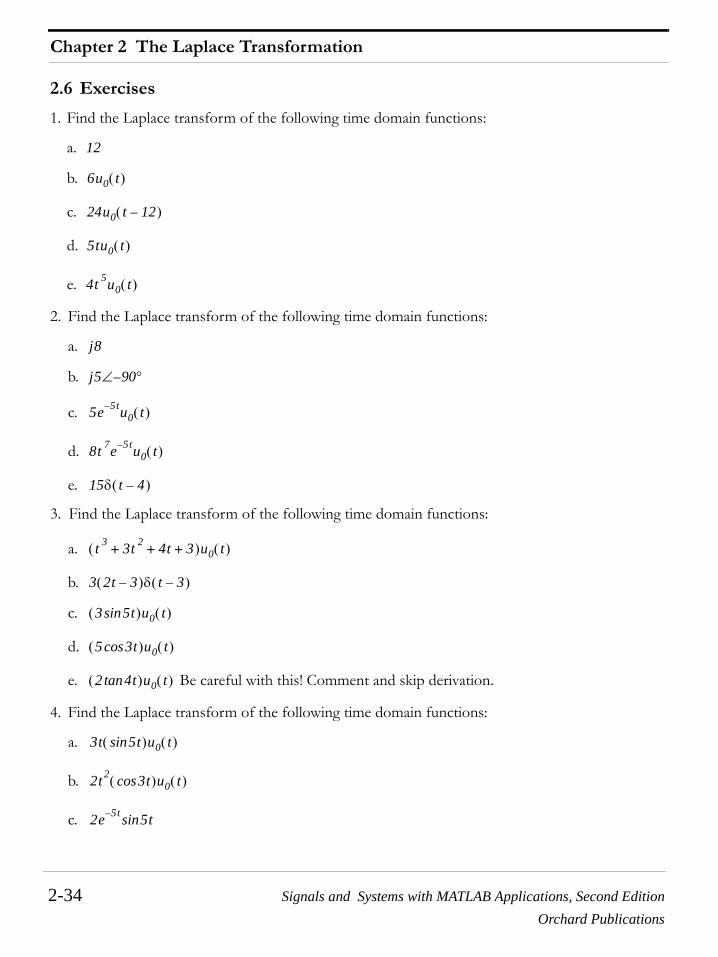
d.
e.
5. Find the Laplace transform of the following time domain functions:
a.
b.
c.
d.
e.
6. Find the Laplace transform of the following time domain functions:
a.
b.
c.
d.
e.
7. Find the Laplace transform of the following time domain functions:
a.
b.
c.
d.
8e 3t– 4tcos
tcos( )δ t π 4⁄–( )
5tu0 t 3–( )
2t 2 5t 4+–( )u0 t 3–( )
t 3–( )e 2t– u0 t 2–( )
2t 4–( )e 2 t 2–( )u0 t 3–( )
4te 3t– 2tcos( )u0 t( )
tdd 3tsin( )
tdd 3e 4t–( )
tdd t 2 2tcos( )
tdd e 2t– 2tsin( )
tdd t 2e
2t–( )
tsint
---------
τsinτ
---------- τd0
t
∫
atsint
------------
τcosτ
----------- τdt
∞
∫

Chapter 2 The Laplace Transformation
2-36 Signals and Systems with MATLAB Applications, Second EditionOrchard Publications
e.
8. Find the Laplace transform for the sawtooth waveform of Figure 2.8.
Figure 2.8. Waveform for Exercise 8.
9. Find the Laplace transform for the full rectification waveform of Figure 2.9.
Figure 2.9. Waveform for Exercise 9
e τ–
τ------- τd
t
∞
∫
fST t( )
A
a 2at
fST t( )
3a
fFR t( )
Full Rectified Waveformsint
1
a 2a 3a 4a
fFR t( )
Chapter 3 The Inverse Laplace Transformation
3-20 Signals and Systems with MATLAB Applications, Second EditionOrchard Publications
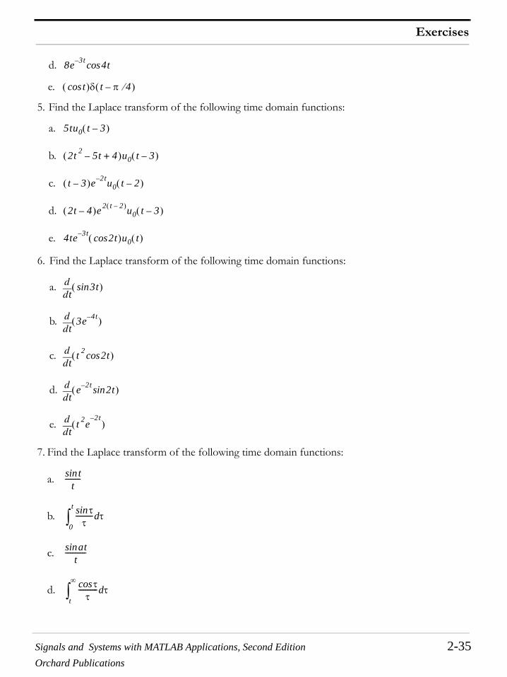
3.6 Exercises
1. Find the Inverse Laplace transform of the following:
a.
b.
c.
d.
e.
2. Find the Inverse Laplace transform of the following:
a.
b.
c.
d.
e.
3. Find the Inverse Laplace transform of the following:
a.
b. (See hint on next page)
4s 3+-----------
4s 3+( )2
------------------
4s 3+( )4
------------------
3s 4+
s 3+( )5------------------
s2 6s 3+ +
s 3+( )5--------------------------
3s 4+
s2 4s 85+ +-----------------------------
4s 5+
s2 5s 18.5+ +---------------------------------
s2 3s 2+ +
s3 5s2 10.5s 9+ + +------------------------------------------------
s2 16–
s3 8s2 24s 32+ + +----------------------------------------------
s 1+
s3 6s2 11s 6+ + +-------------------------------------------
3s 2+
s2 25+-----------------
5s2 3+
s2 4+( )2
---------------------
Signals and Systems with MATLAB Applications, Second Edition 3-21 Orchard Publications
Exercises
Hint:
c.
d.
e.
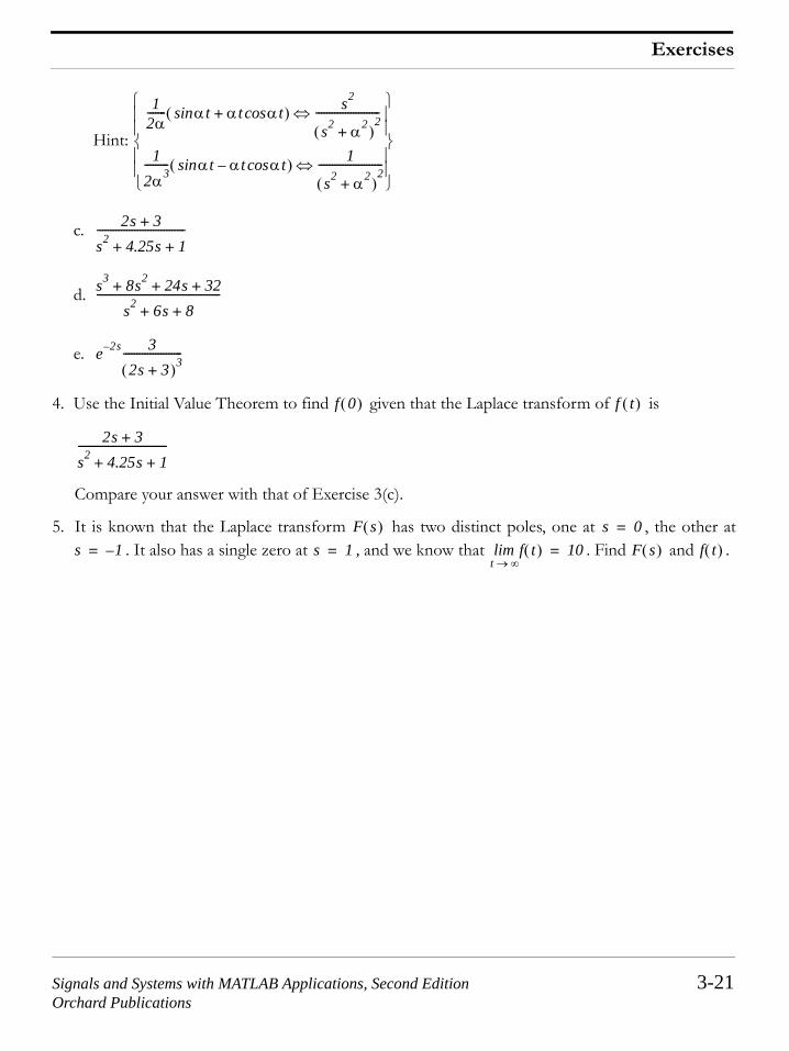
4. Use the Initial Value Theorem to find given that the Laplace transform of is
Compare your answer with that of Exercise 3(c).
5. It is known that the Laplace transform has two distinct poles, one at , the other at. It also has a single zero at , and we know that . Find and .
12α------- αt αt αtcos+sin( ) s2
s2 α2+( )2
------------------------⇔
12α3--------- αtsin αt αtcos–( ) 1
s2 α2+( )2
------------------------⇔⎩ ⎭⎪ ⎪⎪ ⎪⎨ ⎬⎪ ⎪⎪ ⎪⎧ ⎫
2s 3+
s2 4.25s 1+ +---------------------------------
s3 8s2 24s 32+ + +
s2 6s 8+ +----------------------------------------------
e 2s– 32s 3+( )3
----------------------
f 0( ) f t( )
2s 3+
s2 4.25s 1+ +---------------------------------
F s( ) s 0=
s 1–= s 1= f t( )t ∞→lim 10= F s( ) f t( )
Chapter 4 Circuit Analysis with Laplace Transforms
4-18 Signals and Systems with MATLAB Applications, Second EditionOrchard Publications
4.6 Exercises
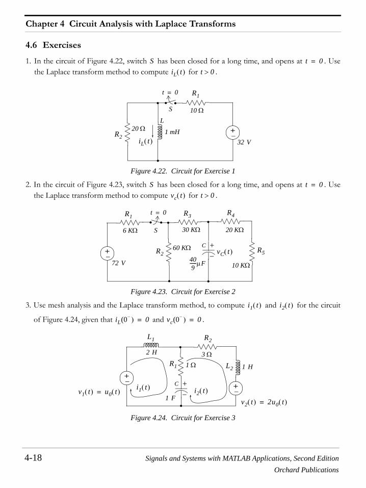
1. In the circuit of Figure 4.22, switch has been closed for a long time, and opens at . Usethe Laplace transform method to compute for .
Figure 4.22. Circuit for Exercise 1
2. In the circuit of Figure 4.23, switch has been closed for a long time, and opens at . Usethe Laplace transform method to compute for .
Figure 4.23. Circuit for Exercise 2
3. Use mesh analysis and the Laplace transform method, to compute and for the circuit
of Figure 4.24, given that and .
Figure 4.24. Circuit for Exercise 3
S t 0=
iL t( ) t 0>
1 mH
S
t 0=
iL t( )+−
L
32 V
10 Ω
20 Ω
R1
R2
S t 0=
vc t( ) t 0>
S
t 0=
+−
72 V
6 KΩ
C
−+60 KΩ
30 KΩ 20 KΩ
10 KΩ409------µF
vC t( )
R1
R2
R3 R4
R5
i1 t( ) i2 t( )
iL(0− ) 0= vc(0− ) 0=
+− C
−+
1 Ω3 Ω
1 Fi1 t( ) +
−
1 H
v1 t( ) u0 t( )=v2 t( ) 2u0 t( )=
2 H
i2 t( )
L1
R1
R2
L2
Signals and Systems with MATLAB Applications, Second Edition 4-19Orchard Publications
Exercises
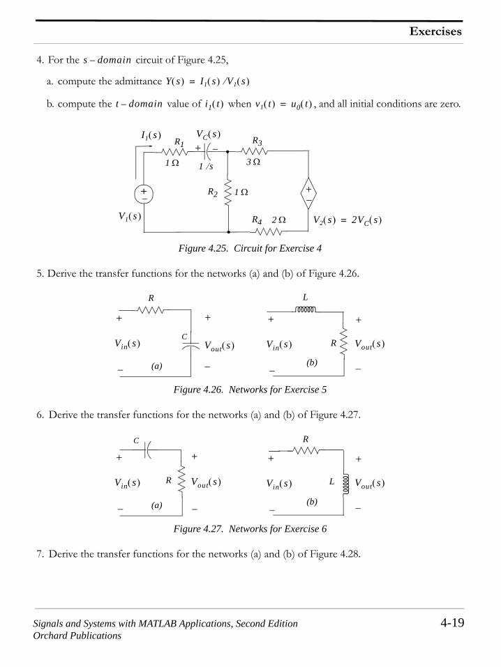
4. For the circuit of Figure 4.25,
a. compute the admittance
b. compute the value of when , and all initial conditions are zero.
Figure 4.25. Circuit for Exercise 4
5. Derive the transfer functions for the networks (a) and (b) of Figure 4.26.
Figure 4.26. Networks for Exercise 5
6. Derive the transfer functions for the networks (a) and (b) of Figure 4.27.
Figure 4.27. Networks for Exercise 6
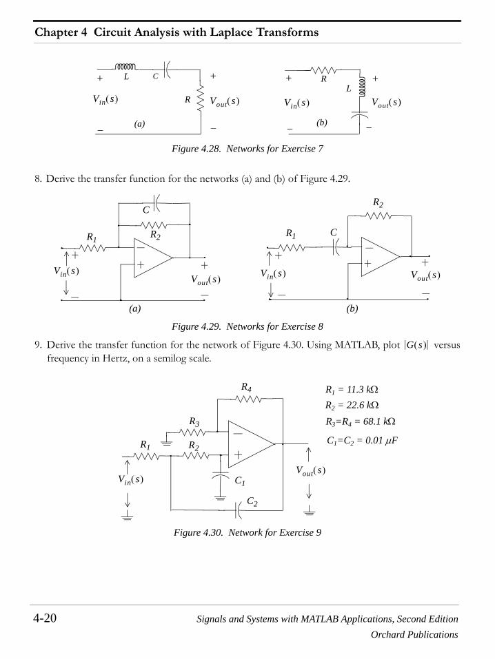
7. Derive the transfer functions for the networks (a) and (b) of Figure 4.28.
s domain–
Y s( ) I1 s( ) V1 s( )⁄=
t domain– i1 t( ) v1 t( ) u0 t( )=
R1
R2+−
1 Ω
+
R3
1 Ω
3 Ω1 s⁄
V1 s( )
−
VC s( )I1 s( )
+−
V2 s( ) 2VC s( )=2 ΩR4
R
C
−
++
−
Vin s( ) Vout s( ) R
L
+
−
Vin s( )
−
+
Vout s( )
(a) (b)
R
C
−
++
−
Vin s( ) Vout s( )
R
L
+
−
Vin s( )
−
+
Vout s( )
(a) (b)
Chapter 4 Circuit Analysis with Laplace Transforms
4-20 Signals and Systems with MATLAB Applications, Second EditionOrchard Publications
Figure 4.28. Networks for Exercise 7
8. Derive the transfer function for the networks (a) and (b) of Figure 4.29.
Figure 4.29. Networks for Exercise 8
9. Derive the transfer function for the network of Figure 4.30. Using MATLAB, plot versusfrequency in Hertz, on a semilog scale.
Figure 4.30. Network for Exercise 9
R
C
−
++
−
Vin s( ) Vout s( )
RL
+
−
Vin s( )
−
+
Vout s( )
(a) (b)
L
R2R1
C
R1
Vin s( )Vout s( )
R2
C
Vin s( ) Vout s( )
(a) (b)
G s( )
R1 R2
R3
C1
C2
Vout s( )Vin s( )
R4 R1 = 11.3 kΩ
R2 = 22.6 kΩ
R3=R4 = 68.1 kΩ
C1=C2 = 0.01 µF
Chapter 6 The Impulse Response and Convolution
6-22 Signals and Systems with MATLAB Applications, Second EditionOrchard Publications
6.7 Exercises
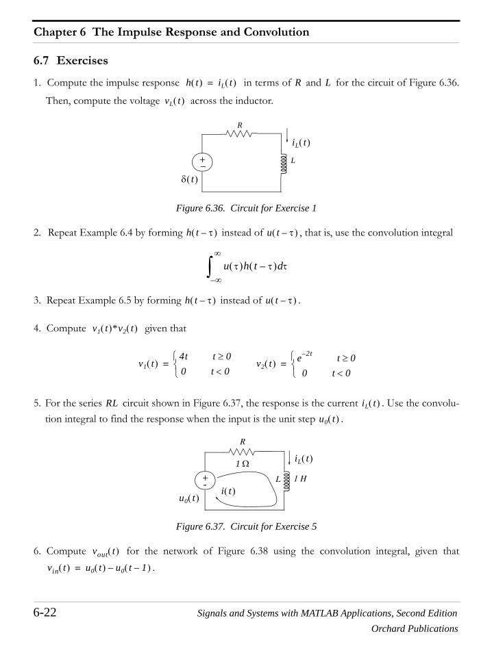
1. Compute the impulse response in terms of and for the circuit of Figure 6.36.
Then, compute the voltage across the inductor.
Figure 6.36. Circuit for Exercise 1
2. Repeat Example 6.4 by forming instead of , that is, use the convolution integral
3. Repeat Example 6.5 by forming instead of .
4. Compute given that
5. For the series circuit shown in Figure 6.37, the response is the current . Use the convolu-tion integral to find the response when the input is the unit step .
Figure 6.37. Circuit for Exercise 5
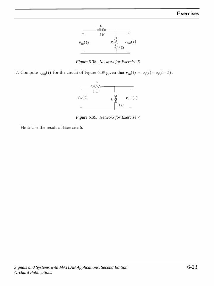
6. Compute for the network of Figure 6.38 using the convolution integral, given that.
h t( ) iL t( )= R L
vL t( )
+−
R
L
iL t( )
δ t( )
h t τ–( ) u t τ–( )
u τ( )h t τ–( ) τd∞–
∞
∫h t τ–( ) u t τ–( )
v1 t( )*v2 t( )
v1 t( )4t t 0≥0 t 0<⎩
⎨⎧
= v2 t( ) e 2t– t 0≥0 t 0<⎩
⎨⎧
=
RL iL t( )
u0 t( )
+- 1 H
R
iL t( )
u0 t( )
L
1 Ω
i t( )
vout t( )
vin t( ) u0 t( ) u0 t 1–( )–=
Signals and Systems with MATLAB Applications, Second Edition 6-23Orchard Publications
Exercises
Figure 6.38. Network for Exercise 6
7. Compute for the circuit of Figure 6.39 given that .
Figure 6.39. Network for Exercise 7
Hint: Use the result of Exercise 6.
R
L
+
−
1 H +
−1 Ω
vin t( ) vout t( )
vout t( ) vin t( ) u0 t( ) u0 t 1–( )–=
R
L
1 H
+ +
− −
vin t( ) vout t( )1 Ω
Signals and Systems with MATLAB Applications, Second Edition 7-51Orchard Publications
Exercises
7.14 Exercises
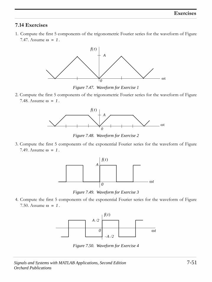
1. Compute the first 5 components of the trigonometric Fourier series for the waveform of Figure7.47. Assume .
Figure 7.47. Waveform for Exercise 1
2. Compute the first 5 components of the trigonometric Fourier series for the waveform of Figure7.48. Assume .
Figure 7.48. Waveform for Exercise 2
3. Compute the first 5 components of the exponential Fourier series for the waveform of Figure7.49. Assume .
Figure 7.49. Waveform for Exercise 3
4. Compute the first 5 components of the exponential Fourier series for the waveform of Figure7.50. Assume .
Figure 7.50. Waveform for Exercise 4
ω 1=
0 ωt
Af t( )
ω 1=
0ωt
Af t( )
ω 1=
0ωt
Af t( )
ω 1=
0 ωt
f t( )A 2⁄
A– 2⁄
Chapter 7 Fourier Series
7-52 Signals and Systems with MATLAB Applications, Second EditionOrchard Publications
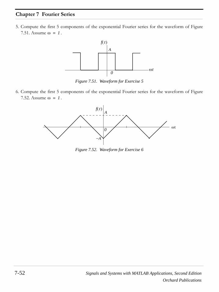
5. Compute the first 5 components of the exponential Fourier series for the waveform of Figure7.51. Assume .
Figure 7.51. Waveform for Exercise 5
6. Compute the first 5 components of the exponential Fourier series for the waveform of Figure7.52. Assume .
Figure 7.52. Waveform for Exercise 6
ω 1=
0ωt
A
f t( )
ω 1=
0 ωt
A
−A
f t( )
Signals and Systems with MATLAB Applications, Second Edition 8-47Orchard Publications
Exercises
8.10 Exercises
1. Show that
2. Compute
3. Sketch the time and frequency waveforms of
4. Derive the Fourier transform of
5. Derive the Fourier transform of
6. Derive the Fourier transform of
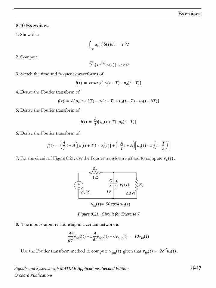
7. For the circuit of Figure 8.21, use the Fourier transform method to compute .
Figure 8.21. Circuit for Exercise 7
8. The input-output relationship in a certain network is
Use the Fourier transform method to compute given that .
u0 t( )δ t( ) td∞–
∞
∫ 1 2⁄=
F te at– u0 t( ) a 0>
f t( ) ω0tcos u0 t T+( ) u0 t T–( )–[ ]=
f t( ) A u0 t 3T+( ) u0 t T+( )– u0 t T–( ) u0 t 3T–( )–+[ ]=
f t( ) AT---t u0 t T+( ) u0– t T–( )[ ]=
f t( ) AT--- t A+⎝ ⎠
⎛ ⎞ u0 t T+( ) u0 t( )–[ ] AT---– t A+⎝ ⎠
⎛ ⎞ u0 t( ) u0 t T2---–⎝ ⎠
⎛ ⎞–+=
vC t( )
+− −
+C
1 Fvin t( )
vC t( )
1 Ω
0.5 Ω
R1
R2
vin t( ) 50 4tucos 0 t( )=
d 2
dt2-------vout t( ) 5 d
dt-----vout t( ) 6vout t( )+ + 10vin t( )=
vout t( ) vin t( ) 2e t– u0 t( )=
Chapter 8 The Fourier Transform
8-48 Signals and Systems with MATLAB Applications, Second EditionOrchard Publications
9. In a bandpass filter, the lower and upper cutoff frequencies are , and respec-tively. Compute the energy of the input, and the percentage that appears at the output, if the
input signal is volts.
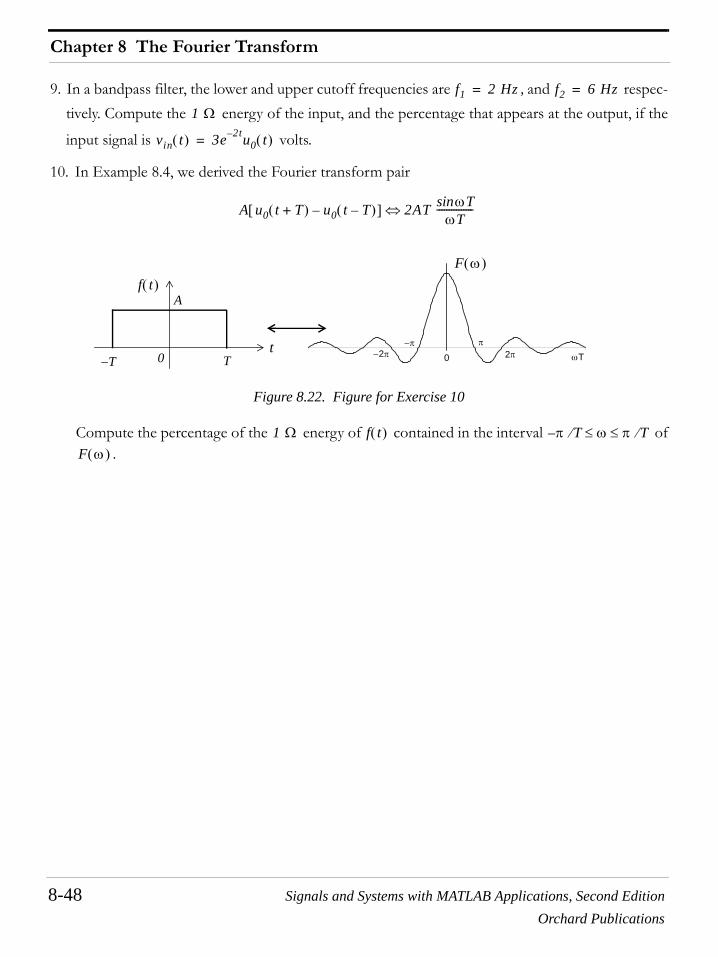
10. In Example 8.4, we derived the Fourier transform pair
Figure 8.22. Figure for Exercise 10
Compute the percentage of the energy of contained in the interval of.
f1 2 Hz= f2 6 Hz=
1 Ω
vin t( ) 3e 2t– u0 t( )=
A u0 t T+( ) u0 t T–( )–[ ] 2AT ωTsinωT
---------------⇔
0 ωT−2π 2ππ−π
A
−T Tt
0
f t( )F ω( )
1 Ω f t( ) π T⁄– ω π T⁄≤ ≤F ω( )
Chapter 9 Discrete Time Systems and the Z Transform
9-52 Signals and Systems with MATLAB Applications, Second EditionOrchard Publications
9.10 Exercises
1. Find the Z transform of the discrete time pulse defined as
2. Find the Z transform of where is defined as in Exercise 1.
3. Prove the following Z transform pairs:
a.
b.
c.
d.
e.
4. Use the partial fraction expansion to find given that
5. Use the partial fraction expansion method to compute the Inverse Z transform of
6. Use the Inversion Integral to compute the Inverse Z transform of
7. Use the long division method to compute the first 5 terms of the discrete time sequence whose Ztransform is
p n[ ]
p n[ ]1 n 0 1 2 … m 1–, , , ,=
0 otherwise⎩⎨⎧
=
anp n[ ] p n[ ]
δ n[ ] 1⇔
δ n 1–[ ] z m–⇔
nanu0 n[ ] azz a–( )2
------------------⇔
n2anu0 n[ ] az z a+( )
z a–( )3----------------------⇔
n 1+[ ]u0 n[ ] z2
z 1–( )2------------------⇔
f n[ ] Z1– F z( )[ ]=
F z( ) A1 z 1––( ) 1 0.5z 1––( )
--------------------------------------------------=
F z( ) z2
z 1+( ) z 0.75–( )2-------------------------------------------=
F z( ) 1 2z 1– z 3–+ +
1 z 1––( ) 1 0.5z 1––( )--------------------------------------------------=
F z( ) z 1– z 2– z 3––+
1 z 1– z 2– 4z 3–+ + +----------------------------------------------=
Signals and Systems with MATLAB Applications, Second Edition 9-53Orchard Publications
Exercises
8. a. Compute the transfer function of the difference equation
b. Compute the response when the input is
9. Given the difference equation
a. Compute the discrete transfer function
b. Compute the response to the input
10. A discrete time system is described by the difference equation
where
a. Compute the transfer function
b. Compute the impulse response
c. Compute the response when the input is
11. Given the discrete transfer function
write the difference equation that relates the output to the input .
y n[ ] y n 1–[ ]– Tx n 1–[ ]=
y n[ ] x n[ ] e naT–=
y n[ ] y n 1–[ ]–T2--- x n[ ] x n 1–[ ]+ =
H z( )
x n[ ] e naT–=
y n[ ] y n 1–[ ]+ x n[ ]=
y n[ ] 0 for n 0<=
H z( )
h n[ ]
x n[ ] 10 for n 0≥=
H z( ) z 2+
8z2 2z– 3–----------------------------=
y n[ ] x n[ ]
Signals and Systems with MATLAB Applications, Second Edition 10-31Orchard Publications
Exercises
10.8 Exercises
1. Compute the DFT of the sequence ,
2. A square waveform is represented by the discrete time sequence
and
Use MATLAB to compute and plot the magnitude of this sequence.
3. Prove that
a.
b.
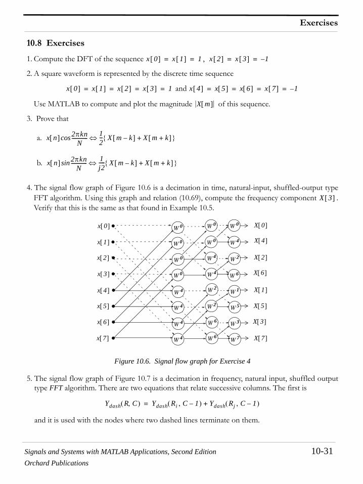
4. The signal flow graph of Figure 10.6 is a decimation in time, natural-input, shuffled-output typeFFT algorithm. Using this graph and relation (10.69), compute the frequency component .Verify that this is the same as that found in Example 10.5.
Figure 10.6. Signal flow graph for Exercise 4
5. The signal flow graph of Figure 10.7 is a decimation in frequency, natural input, shuffled outputtype FFT algorithm. There are two equations that relate successive columns. The first is
and it is used with the nodes where two dashed lines terminate on them.
x 0[ ] x 1[ ] 1= = x 2[ ] x 3[ ] 1–= =
x 0[ ] x 1[ ] x 2[ ] x 3[ ] 1= = = = x 4[ ] x 5[ ] x 6[ ] x 7[ ] 1–= = = =
X m[ ]
x n[ ] 2πknN
-------------cos 12--- X m k–[ ] X m k+[ ]+ ⇔
x n[ ] 2πknN
-------------sin 1j2----- X m k–[ ] X m k+[ ]+ ⇔
X 3[ ]
W 0
W 0
W 0
W 0
W 4
W 4
W 4
W 4
W 0
W 4
W 2
W 1
W 0
W 4
W 4
W 2
W 2
W 6
W 6
W 0
W 6
W 5
W 3
W 7
x 0[ ]
x 1[ ]
x 2[ ]
x 3[ ]
x 4[ ]
x 5[ ]
x 6[ ]
x 7[ ] X 7[ ]
X 3[ ]
X 5[ ]
X 1[ ]
X 0[ ]
X 4[ ]
X 2[ ]
X 6[ ]
Ydash R C,( ) Ydash Ri C 1–,( ) Ydash Rj C 1–,( )+=
Chapter 10 The DFT and the FFT Algorithm
10-32 Signals and Systems with MATLAB Applications, Second EditionOrchard Publications
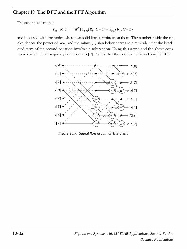
The second equation is
and it is used with the nodes where two solid lines terminate on them. The number inside the cir-cles denote the power of , and the minus (−) sign below serves as a reminder that the brack-eted term of the second equation involves a subtraction. Using this graph and the above equa-tions, compute the frequency component . Verify that this is the same as in Example 10.5.
Figure 10.7. Signal flow graph for Exercise 5
Ysol R C,( ) W m Ysol Ri C 1–,( ) Ysol Rj C 1–,( )–[ ]=
WN
X 3[ ]
W 0
W 1
W 2
W 3
W 0
W 0
W 2
W 0
W 2
W 0
W 0
W 0
x 0[ ]
x 1[ ]
x 2[ ]
x 3[ ]
x 4[ ]
x 5[ ]
x 6[ ]
x 7[ ] X 7[ ]
X 3[ ]
X 5[ ]
X 1[ ]
X 0[ ]
X 4[ ]
X 2[ ]
X 6[ ]
−
−
− −
−
− −
− −
− − −
Signals and Systems with MATLAB Applications, Second Edition 11-73Orchard Publications
Exercises
11.10 Exercises
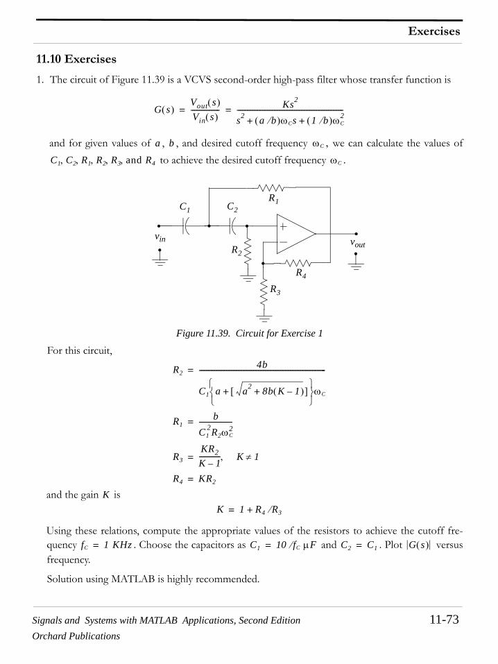
1. The circuit of Figure 11.39 is a VCVS second-order high-pass filter whose transfer function is
and for given values of , , and desired cutoff frequency , we can calculate the values of to achieve the desired cutoff frequency .
Figure 11.39. Circuit for Exercise 1
For this circuit,
and the gain is
Using these relations, compute the appropriate values of the resistors to achieve the cutoff fre-quency . Choose the capacitors as and . Plot versusfrequency.
Solution using MATLAB is highly recommended.
G s( )Vout s( )Vin s( )----------------- Ks2
s2 a b⁄( )ωCs 1 b⁄( )ωC2+ +
---------------------------------------------------------------= =
a b ωC
C1 C2 R1 R2 R3 and R4, , , , , ωC
vin vout
C1 C2
R2
R1
R3
R4
R24b
C1 a a2 8b K 1–( )+[ ]+⎩ ⎭⎨ ⎬⎧ ⎫
ωC
---------------------------------------------------------------------------=
R1b
C12R2ωC
2--------------------=
R3KR2K 1–------------- K 1≠,=
R4 KR2=
KK 1 R4 R3⁄+=
fC 1 KHz= C1 10 fC⁄ µF= C2 C1= G s( )
Chapter 11 Analog and Digital Filters
11-74 Signals and Systems with MATLAB Applications, Second EditionOrchard Publications
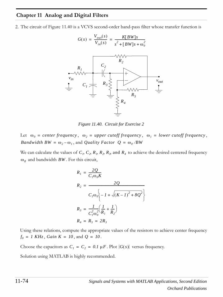
2. The circuit of Figure 11.40 is a VCVS second-order band-pass filter whose transfer function is
Figure 11.40. Circuit for Exercise 2
Let , , ,, and
We can calculate the values of to achieve the desired centered frequency and bandwidth . For this circuit,
Using these relations, compute the appropriate values of the resistors to achieve center frequency, , and .
Choose the capacitors as . Plot versus frequency.
Solution using MATLAB is highly recommended.
G s( )Vout s( )Vin s( )----------------- K BW[ ]s
s2 BW[ ]s ω02+ +
----------------------------------------= =
vin voutC1
R5
C2
R3
R2
R1
R4
ω0 center frequency= ω2 upper cutoff frequency= ω1 lower cutoff frequency=
Bandwidth BW ω2 ω1–= Quality Factor Q ω0 BW⁄=
C1 C2 R1 R2 R3 and R4, , , , ,
ω0 BW
R12Q
C1ω0K-----------------=
R22Q
C1ω0 1– K 1–( )2 8Q2++⎩ ⎭⎨ ⎬⎧ ⎫
--------------------------------------------------------------------------=
R31
C12ω0
2------------- 1
R1----- 1
R2-----+⎝ ⎠
⎛ ⎞ =
R4 R5 2R3= =
f0 1 KHz= Gain K 10= Q 10=
C1 C2 0.1 µF= = G s( )
Signals and Systems with MATLAB Applications, Second Edition 11-75Orchard Publications
Exercises
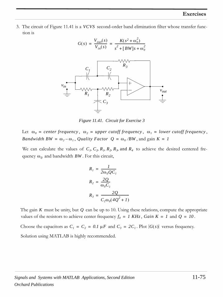
3. The circuit of Figure 11.41 is a second-order band elimination filter whose transfer func-tion is
Figure 11.41. Circuit for Exercise 3
Let , , ,, , and gain
We can calculate the values of to achieve the desired centered fre-quency and bandwidth . For this circuit,
The gain must be unity, but can be up to 10. Using these relations, compute the appropriatevalues of the resistors to achieve center frequency , and .
Choose the capacitors as and . Plot versus frequency.
Solution using MATLAB is highly recommended.
VCVS
G s( )Vout s( )Vin s( )----------------- K s2 ω0
2+( )
s2 BW[ ]s ω02+ +
----------------------------------------= =
vinvout
C2C1R3
R1 R2
C3
ω0 center frequency= ω2 upper cutoff frequency= ω1 lower cutoff frequency=
Bandwidth BW ω2 ω1–= Quality Factor Q ω0 BW⁄= K 1=
C1 C2 R1 R2 R3 and R4, , , , ,
ω0 BW
R11
2ω0QC1--------------------=
R22Q
ω0C1------------=
R32Q
C1ω0 4Q2 1+( )------------------------------------- =
K Qf0 1 KHz= Gain K 1= Q 10=
C1 C2 0.1 µF= = C3 2C1= G s( )
Chapter 11 Analog and Digital Filters
11-76 Signals and Systems with MATLAB Applications, Second EditionOrchard Publications
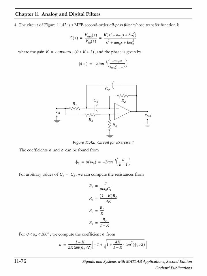
4. The circuit of Figure 11.42 is a MFB second-order all-pass filter whose transfer function is
where the gain , , and the phase is given by
Figure 11.42. Circuit for Exercise 4
The coefficients and can be found from
For arbitrary values of , we can compute the resistances from
For , we compute the coefficient from
G s( )Vout s( )Vin s( )-----------------
K s2 aω0s– bω02+( )
s2 aω0s bω02+ +
----------------------------------------------= =
K cons ttan= 0 K 1< <( )
φ ω( ) 2tan 1– aω0ω
bω02 ω2–
----------------------⎝ ⎠⎛ ⎞–=
vin vout
C1
C2
R1R2
R4
R3
a b
φ0 φ ω0( ) 2tan 1– ab 1–------------⎝ ⎠
⎛ ⎞–= =
C1 C2=
R22
aω0C1----------------=
R11 K–( )R2
4K------------------------=
R3R2
K----- =
R4R2
1 K–------------- =
0 φ0 180°< < a
a 1 K–2K φ0 2⁄( )tan--------------------------------- 1– 1 4K
1 K–------------- tan2 φ0 2⁄( )⋅++=
Signals and Systems with MATLAB Applications, Second Edition 11-77Orchard Publications
Exercises
and for , from
Using these relations, compute the appropriate values of the resistors to achieve a phase shift at with .
Choose the capacitors as and plot phase versus frequency.
Solution using MATLAB is highly recommended.
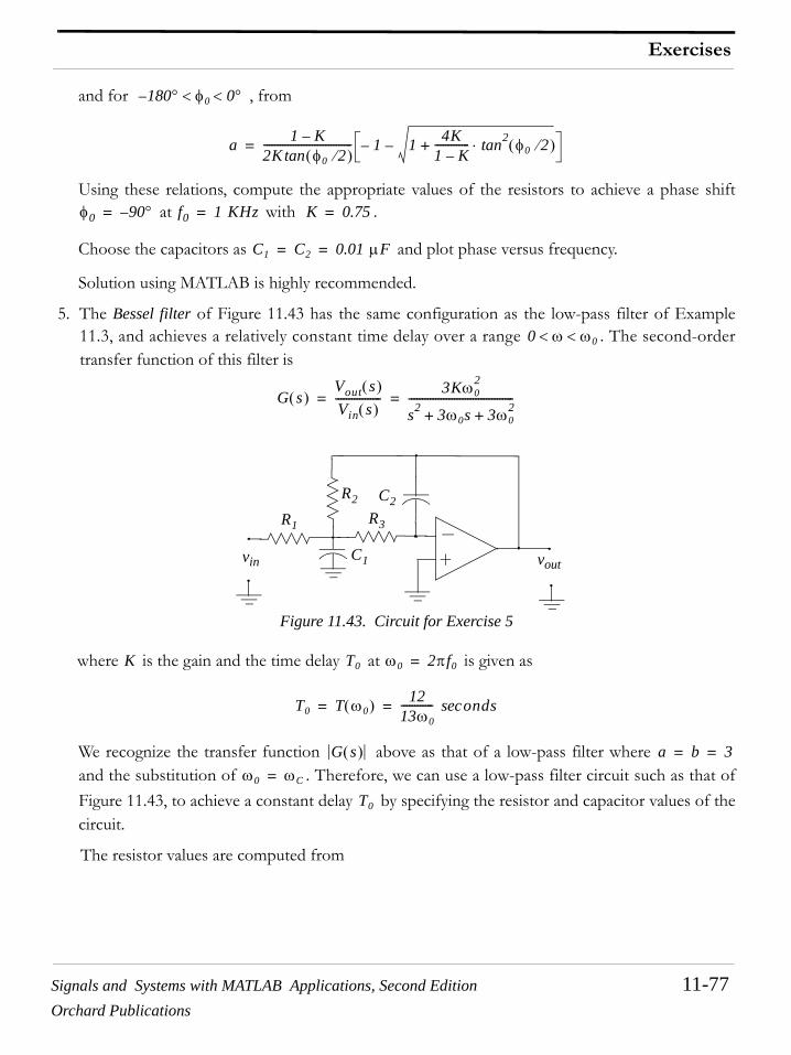
5. The Bessel filter of Figure 11.43 has the same configuration as the low-pass filter of Example11.3, and achieves a relatively constant time delay over a range . The second-ordertransfer function of this filter is
Figure 11.43. Circuit for Exercise 5
where is the gain and the time delay at is given as
We recognize the transfer function above as that of a low-pass filter where and the substitution of . Therefore, we can use a low-pass filter circuit such as that ofFigure 11.43, to achieve a constant delay by specifying the resistor and capacitor values of thecircuit.
The resistor values are computed from
180°– φ0 0°< <
a 1 K–2K φ0 2⁄( )tan--------------------------------- 1– 1 4K
1 K–------------- tan2 φ0 2⁄( )⋅+–=
φ0 90°–= f0 1 KHz= K 0.75=
C1 C2 0.01 µF= =
0 ω ω0< <
G s( )Vout s( )Vin s( )----------------- 3Kω0
2
s2 3ω0s 3ω02+ +
---------------------------------------= =
vin voutC1
C2R2
R1 R3
K T0 ω0 2πf0=
T0 T ω0( ) 1213ω0------------ ondssec= =
G s( ) a b 3= =
ω0 ωC=
T0
Chapter 11 Analog and Digital Filters
11-78 Signals and Systems with MATLAB Applications, Second EditionOrchard Publications
Using these relations, compute the appropriate values of the resistors to achieve a time delay with . Use capacitors and . Plot versus
frequency.
Solution using MATLAB is highly recommended.
6. Derive the transfer function of a fourth-order Butterworth filter with .
7. Derive the amplitude-squared function for a third-order Type I Chebyshev low-pass filter with pass band ripple and cutoff frequency .
8. Use MATLAB to derive the transfer function and plot versus for a two-pole, TypeI Chebyshev high-pass digital filter with sampling period . The equivalent analog filtercutoff frequency is and has pass band ripple. Compute the coefficients ofthe numerator and denominator and plot with and without pre-warping.
R22 K 1+( )
aC1 a2C12 4– bC1C2 K 1–( )+( )ω0
------------------------------------------------------------------------------------=
R1R2
K-----=
R31
bC1C2R2ω02
-----------------------------=
T0 100 µs= K 2= C1 0.01 µF= C2 0.002 µF= G s( )
ωC 1 rad s⁄=
1.5 dB ωC 1 rad s⁄=
G z( ) G z( ) ωTS 0.25 s=
ωC 4 rad s⁄= 3 dB
G z( )