Embed Size (px)
Citation preview
Chapter 1 Consumer Theory Part IIEconomics 5113 Microeconomic Theory
Kam Yu
Winter 2019
Outline
1 Introduction to Duality TheoryIndirect Utility and Expenditure FunctionsOrdinary and Compensated Demand Functions
2 Properties of Consumer DemandRelative Prices and Real IncomeIncome and Substitution EffectsImplications
3 ElasticitiesDefinitionsAverage Elasticities
Kam Yu (Lakehead) Chapter 1 Consumer Theory Part II Winter 2019 2 / 25
Introduction to Duality Theory Indirect Utility and Expenditure Functions
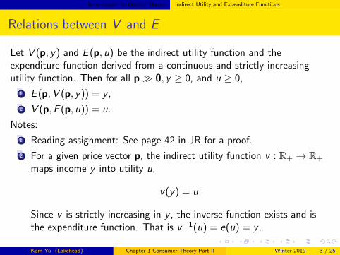
Relations between V and E
Let V (p, y) and E (p, u) be the indirect utility function and theexpenditure function derived from a continuous and strictly increasingutility function. Then for all p� 0, y ≥ 0, and u ≥ 0,
1 E (p,V (p, y)) = y ,
2 V (p,E (p, u)) = u.
Notes:
1 Reading assignment: See page 42 in JR for a proof.
2 For a given price vector p, the indirect utility function v : R+ → R+
maps income y into utility u,
v(y) = u.
Since v is strictly increasing in y , the inverse function exists and isthe expenditure function. That is v−1(u) = e(u) = y .
Kam Yu (Lakehead) Chapter 1 Consumer Theory Part II Winter 2019 3 / 25
Introduction to Duality Theory Indirect Utility and Expenditure Functions
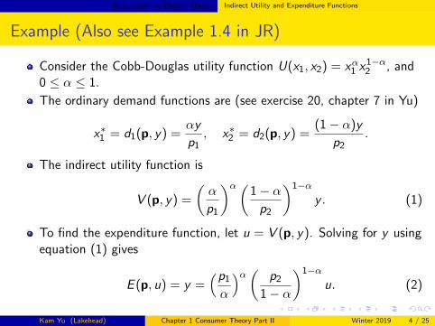
Example (Also see Example 1.4 in JR)
Consider the Cobb-Douglas utility function U(x1, x2) = xα1 x1−α2 , and
0 ≤ α ≤ 1.
The ordinary demand functions are (see exercise 20, chapter 7 in Yu)
x∗1 = d1(p, y) =αy
p1, x∗2 = d2(p, y) =
(1− α)y
p2.
The indirect utility function is
V (p, y) =
(α
p1
)α(1− αp2
)1−αy . (1)
To find the expenditure function, let u = V (p, y). Solving for y usingequation (1) gives
E (p, u) = y =(p1
α
)α( p2
1− α
)1−αu. (2)
Kam Yu (Lakehead) Chapter 1 Consumer Theory Part II Winter 2019 4 / 25
Introduction to Duality Theory Ordinary and Compensated Demand Functions
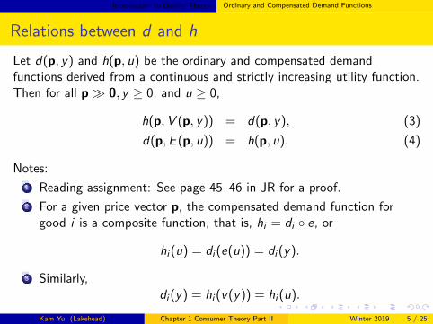
Relations between d and h
Let d(p, y) and h(p, u) be the ordinary and compensated demandfunctions derived from a continuous and strictly increasing utility function.Then for all p� 0, y ≥ 0, and u ≥ 0,
h(p,V (p, y)) = d(p, y), (3)
d(p,E (p, u)) = h(p, u). (4)
Notes:
1 Reading assignment: See page 45–46 in JR for a proof.
2 For a given price vector p, the compensated demand function forgood i is a composite function, that is, hi = di ◦ e, or
hi (u) = di (e(u)) = di (y).
3 Similarly,di (y) = hi (v(y)) = hi (u).
Kam Yu (Lakehead) Chapter 1 Consumer Theory Part II Winter 2019 5 / 25
Introduction to Duality Theory Ordinary and Compensated Demand Functions
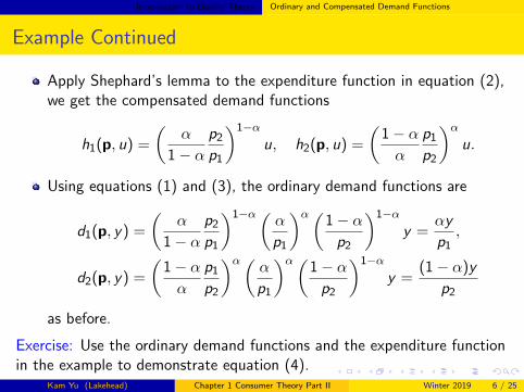
Example Continued
Apply Shephard’s lemma to the expenditure function in equation (2),we get the compensated demand functions
h1(p, u) =
(α
1− αp2
p1
)1−αu, h2(p, u) =
(1− αα
p1
p2
)α
u.
Using equations (1) and (3), the ordinary demand functions are
d1(p, y) =
(α
1− αp2
p1
)1−α( αp1
)α(1− αp2
)1−αy =
αy
p1,
d2(p, y) =
(1− αα
p1
p2
)α( αp1
)α(1− αp2
)1−αy =
(1− α)y
p2
as before.
Exercise: Use the ordinary demand functions and the expenditure functionin the example to demonstrate equation (4).
Kam Yu (Lakehead) Chapter 1 Consumer Theory Part II Winter 2019 6 / 25
Properties of Consumer Demand Relative Prices and Real Income
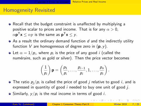
Homogeneity Revisited
Recall that the budget constraint is unaffected by multiplying apositive scalar to prices and income. That is for any α > 0,αpTx ≤ αy is the same as pTx ≤ y .
As a result the ordinary demand function d and the indirectly utilityfunction V are homogeneous of degree zero in (p, y).
Let α = 1/pi , where pi is the price of any good i (called thenumeraire, such as gold or silver). Then the price vector becomes(
1
pi
)p =
(p1
pi, . . . ,
pi−1
pi, 1, . . . ,
pnpi
).
The ratio pj/pi is called the price of good j relative to good i , and isexpressed in quantity of good i needed to buy one unit of good j .
Similarly, y/pi is the real income in terms of good i .
Kam Yu (Lakehead) Chapter 1 Consumer Theory Part II Winter 2019 7 / 25
Properties of Consumer Demand Income and Substitution Effects
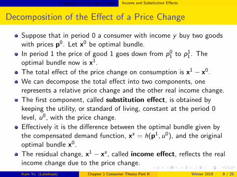
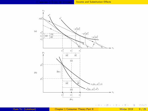
Decomposition of the Effect of a Price Change
Suppose that in period 0 a consumer with income y buy two goodswith prices p0. Let x0 be optimal bundle.
In period 1 the price of good 1 goes down from p01 to p1
1 . Theoptimal bundle now is x1.
The total effect of the price change on consumption is x1 − x0.
We can decompose the total effect into two components, onerepresents a relative price change and the other real income change.
The first component, called substitution effect, is obtained bykeeping the utility, or standard of living, constant at the period 0level, u0, with the price change.
Effectively it is the difference between the optimal bundle given bythe compensated demand function, xs = h(p1, u0), and the originaloptimal bundle x0.
The residual change, x1 − xs , called income effect, reflects the realincome change due to the price change.
Kam Yu (Lakehead) Chapter 1 Consumer Theory Part II Winter 2019 8 / 25
Properties of Consumer Demand Income and Substitution Effects
52 CHAPTER 1
x1
(a)
(b)
x2
x1
p1
x20
x21
x2s
x10
p10
x11
p11
x1s
x10 x1
1x1s
!p10/p2
0
!p11/p2
0
!p11/p2
0
y/p20
u0
u1
SE
SE
TE
TE
IE
IE
SE IE
TE
"x1
"p1
x1h(p1, p2
0, u0)
x1(p1, p20, y)
Figure 1.20. The Hicksian decomposition of a price change.
substitution effects on good 1 and good 2, and we regard them as due ‘purely’ to thechange in relative prices with no change whatsoever in the well-being of the consumer.Look now at what is left of the total effect to explain. After hypothetical changes fromx01 and x
02 to x
s1 and x
s2, the changes from xs1 and x
s2 to x
11 and x
12 remain to be explained.
Notice, however, that these are precisely the consumption changes that would occur if, atthe new prices and the original level of utility u0, the consumer were given an increase inreal income shifting his budget constraint from the hypothetical dashed one out to the final,post price-change line tangent to u1. It is in this sense that the Hicksian income effect cap-tures the change in consumption due ‘purely’ to the income-like change that accompaniesa price change.
Kam Yu (Lakehead) Chapter 1 Consumer Theory Part II Winter 2019 9 / 25
Properties of Consumer Demand Income and Substitution Effects
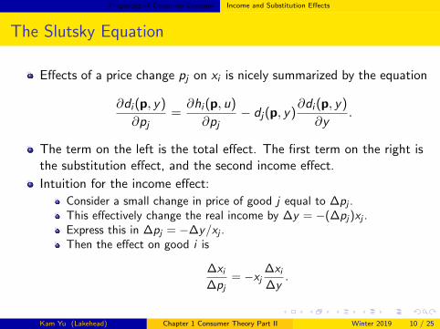
The Slutsky Equation
Effects of a price change pj on xi is nicely summarized by the equation
∂di (p, y)
∂pj=∂hi (p, u)
∂pj− dj(p, y)
∂di (p, y)
∂y.
The term on the left is the total effect. The first term on the right isthe substitution effect, and the second income effect.
Intuition for the income effect:
Consider a small change in price of good j equal to ∆pj .This effectively change the real income by ∆y = −(∆pj)xj .Express this in ∆pj = −∆y/xj .Then the effect on good i is
∆xi∆pj
= −xj∆xi∆y
.
Kam Yu (Lakehead) Chapter 1 Consumer Theory Part II Winter 2019 10 / 25

Properties of Consumer Demand Income and Substitution Effects
Proof of the Slutsky Equation
Recall the duality relation hi (p, u) = di (p,E (p, u)).
Differentiate both sides of the equation with respect to pj :
∂hi (p, u)
∂pj=∂di (p, y)
∂pj+∂di (p, y)
∂y
∂E (p, u)
∂pj. (5)
By Shephard’s lemma, ∂E (p, u)/∂pj = hj(p, u).
At (p, y), the ordinary demand and compensated demand are thesame, that is,
hj(p, u) = dj(p,E (p, u)) = dj(p, y).
Substitute this into the last term in equation (5) and rearrange, weget the Slutsky equation.
Kam Yu (Lakehead) Chapter 1 Consumer Theory Part II Winter 2019 11 / 25
Properties of Consumer Demand Implications
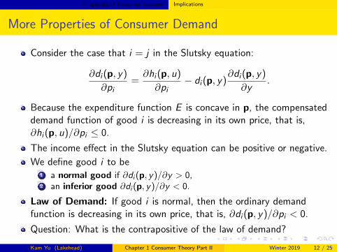
More Properties of Consumer Demand
Consider the case that i = j in the Slutsky equation:
∂di (p, y)
∂pi=∂hi (p, u)
∂pi− di (p, y)
∂di (p, y)
∂y.
Because the expenditure function E is concave in p, the compensateddemand function of good i is decreasing in its own price, that is,∂hi (p, u)/∂pi ≤ 0.
The income effect in the Slutsky equation can be positive or negative.
We define good i to be1 a normal good if ∂di (p, y)/∂y > 0,2 an inferior good ∂di (p, y)/∂y < 0.
Law of Demand: If good i is normal, then the ordinary demandfunction is decreasing in its own price, that is, ∂di (p, y)/∂pi < 0.
Question: What is the contrapositive of the law of demand?
Kam Yu (Lakehead) Chapter 1 Consumer Theory Part II Winter 2019 12 / 25
Properties of Consumer Demand Implications
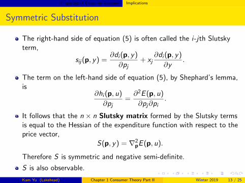
Symmetric Substitution
The right-hand side of equation (5) is often called the i-jth Slutskyterm,
sij(p, y) =∂di (p, y)
∂pj+ xj
∂di (p, y)
∂y.
The term on the left-hand side of equation (5), by Shephard’s lemma,is
∂hi (p, u)
∂pj=∂2E (p, u)
∂pj∂pi.
It follows that the n × n Slutsky matrix formed by the Slutsky termsis equal to the Hessian of the expenditure function with respect to theprice vector,
S(p, y) = ∇2pE (p, u).
Therefore S is symmetric and negative semi-definite.
S is also observable.
Kam Yu (Lakehead) Chapter 1 Consumer Theory Part II Winter 2019 13 / 25
Elasticities Definitions
Income Elasticity of Demand
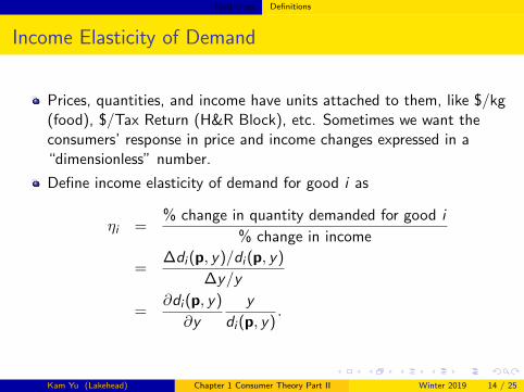
Prices, quantities, and income have units attached to them, like $/kg(food), $/Tax Return (H&R Block), etc. Sometimes we want theconsumers’ response in price and income changes expressed in a“dimensionless” number.
Define income elasticity of demand for good i as
ηi =% change in quantity demanded for good i
% change in income
=∆di (p, y)/di (p, y)
∆y/y
=∂di (p, y)
∂y
y
di (p, y).
Kam Yu (Lakehead) Chapter 1 Consumer Theory Part II Winter 2019 14 / 25
Elasticities Definitions
Properties of Income Elasticity
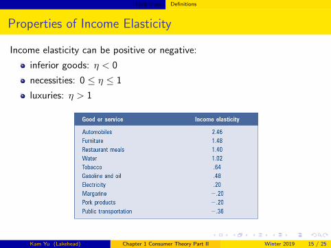
Income elasticity can be positive or negative:
inferior goods: η < 0
necessities: 0 ≤ η ≤ 1
luxuries: η > 1
Kam Yu (Lakehead) Chapter 1 Consumer Theory Part II Winter 2019 15 / 25
Elasticities Definitions
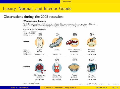
Luxury, Normal, and Inferior Goods
Observations during the 2008 recession:
Kam Yu (Lakehead) Chapter 1 Consumer Theory Part II Winter 2019 16 / 25
Elasticities Definitions
Price Elasticity of Demand
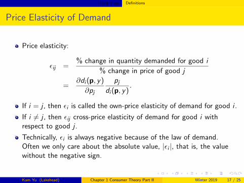
Price elasticity:
εij =% change in quantity demanded for good i
% change in price of good j
=∂di (p, y)
∂pj
pjdi (p, y)
.
If i = j , then εi is called the own-price elasticity of demand for good i .
If i 6= j , then εij cross-price elasticity of demand for good i withrespect to good j .
Technically, εi is always negative because of the law of demand.Often we only care about the absolute value, |εi |, that is, the valuewithout the negative sign.
Kam Yu (Lakehead) Chapter 1 Consumer Theory Part II Winter 2019 17 / 25
Elasticities Definitions
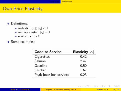
Own-Price Elasticity
Definitions:
inelastic: 0 ≤ |εi | < 1unitary elastic: |εi | = 1elastic: |εi | > 1
Some examples:
Good or Service Elasticity |εi |Cigarettes 0.42Salmon 2.47Gasoline 0.50Chicken 1.67Peak hour bus services 0.23
Kam Yu (Lakehead) Chapter 1 Consumer Theory Part II Winter 2019 18 / 25

Elasticities Definitions
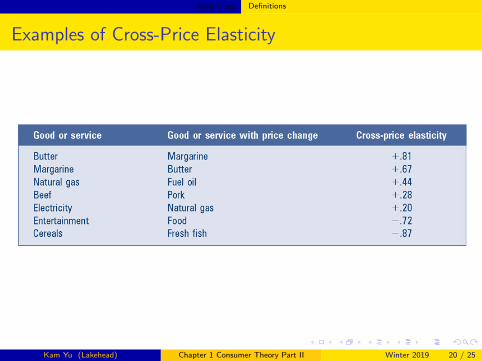
Substitutes and Complements
Two goods are substitutes if the price of one good goes up result in anincrease in demand for the other good. Examples:
Zippers and buttons
Butter and margarine
Natural gas and fuel oil
Pork and chicken
Two goods are complements if the price of one good goes up result in andecrease in demand for the other good. Examples:
Movie tickets and restaurant meals
Lettuce and salad dressing
Blue-ray players and HDTV
Kam Yu (Lakehead) Chapter 1 Consumer Theory Part II Winter 2019 19 / 25
Elasticities Definitions
Examples of Cross-Price Elasticity
Kam Yu (Lakehead) Chapter 1 Consumer Theory Part II Winter 2019 20 / 25
Elasticities Average Elasticities
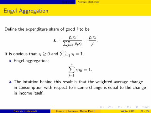
Engel Aggregation
Define the expenditure share of good i to be
si =pixi∑nj=1 pjxj
=pixiy.
It is obvious that si ≥ 0 and∑n
i=1 si = 1.
Engel aggregation:n∑
i=1
siηi = 1.
The intuition behind this result is that the weighted average changein consumption with respect to income change is equal to the changein income itself.
Kam Yu (Lakehead) Chapter 1 Consumer Theory Part II Winter 2019 21 / 25

Elasticities Average Elasticities
Proof of Engel Aggregation
Recall that straight monotonicity of the utility function implies that thebudget constraint is binding. This translates into the so-called budgetbalancedness condition: For all p� 0 and y ≥ 0,
n∑i=1
pidi (p, y) = y . (6)
Differentiate both sides with respect to y , we get
n∑i=1
pi∂di (p, y)
∂y= 1.
Multiply and divide each term on the left by ydi (p, y) gives the result.
Kam Yu (Lakehead) Chapter 1 Consumer Theory Part II Winter 2019 22 / 25
Elasticities Average Elasticities
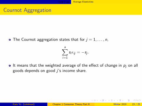
Cournot Aggregation
The Cournot aggregation states that for j = 1, . . . , n,
n∑i=1
siεij = −sj .
It means that the weighted average of the effect of change in pj on allgoods depends on good j ’s income share.
Kam Yu (Lakehead) Chapter 1 Consumer Theory Part II Winter 2019 23 / 25
Elasticities Average Elasticities
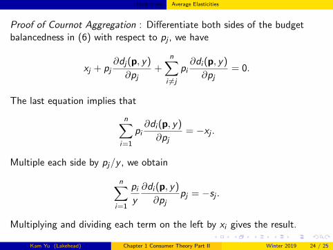
Proof of Cournot Aggregation : Differentiate both sides of the budgetbalancedness in (6) with respect to pj , we have
xj + pj∂dj(p, y)
∂pj+
n∑i 6=j
pi∂di (p, y)
∂pj= 0.
The last equation implies that
n∑i=1
pi∂di (p, y)
∂pj= −xj .
Multiple each side by pj/y , we obtain
n∑i=1
piy
∂di (p, y)
∂pjpj = −sj .
Multiplying and dividing each term on the left by xi gives the result.
Kam Yu (Lakehead) Chapter 1 Consumer Theory Part II Winter 2019 24 / 25

Elasticities Average Elasticities
From Statistics Canada’s Survey of Household Spending
Canadian households spent an average of $62,183 on goods andservices in 2016, up 2.8% from 2015.
Spending on shelter accounted for 29.0% of this total, followed bytransportation (19.2%) and food (14.1%).
Provincially, the highest average spending on goods and services wasreported by households in Alberta ($74,044), followed by Ontario($66,220) and Saskatchewan ($65,411). Households in NewBrunswick ($50,175) reported the lowest average spending.
On average, couples with children spent $88,273 on goods andservices, compared with $34,674 for one-person households.
Kam Yu (Lakehead) Chapter 1 Consumer Theory Part II Winter 2019 25 / 25


![[PPT]Electric Bus Management System - Lakehead Universityflash.lakeheadu.ca/~wchow/Degree Project/Proposal... · Web viewProblem Outline Public transportation faces problems with](https://img.pdfslide.us/doc/110x75/5aecac637f8b9ad73f8ff66f/pptelectric-bus-management-system-lakehead-wchowdegree-projectproposalweb.jpg)