Embed Size (px)
Citation preview
1
Chapter 1
The Production Paradigm
Production Management 2
Evolution of Production Systems
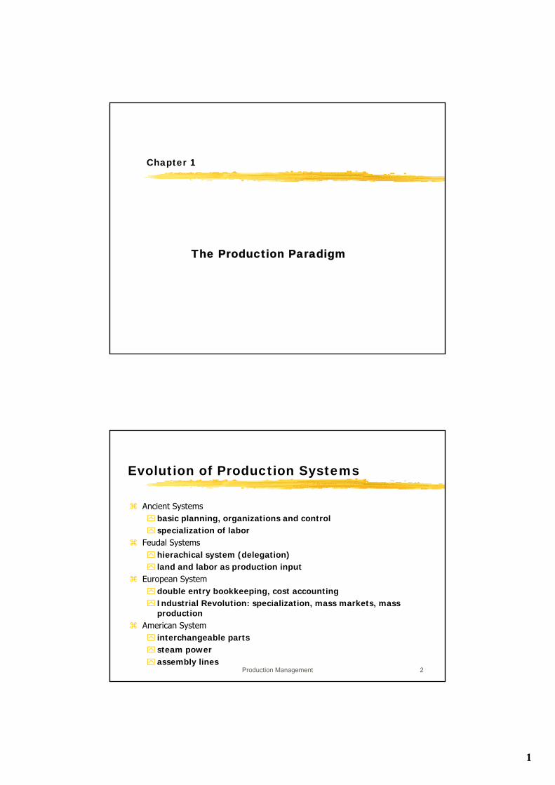
Ancient Systemsbasic planning, organizations and controlspecialization of labor
Feudal Systemshierachical system (delegation)land and labor as production input
European Systemdouble entry bookkeeping, cost accounting Industrial Revolution: specialization, mass markets, mass production
American Systeminterchangeable partssteam powerassembly lines
2
Production Management 3
The Competitive Environment
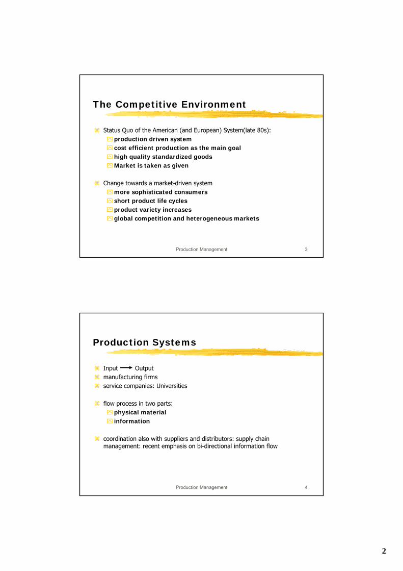
Status Quo of the American (and European) System(late 80s):production driven systemcost efficient production as the main goalhigh quality standardized goodsMarket is taken as given
Change towards a market-driven systemmore sophisticated consumersshort product life cyclesproduct variety increasesglobal competition and heterogeneous markets
Production Management 4
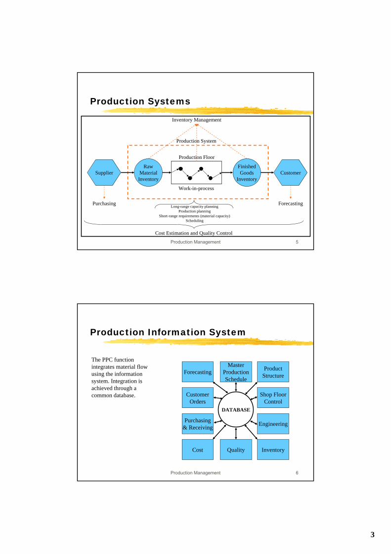
Production Systems
Input Outputmanufacturing firmsservice companies: Universities
flow process in two parts: physical materialinformation
coordination also with suppliers and distributors: supply chain management: recent emphasis on bi-directional information flow
3
Production Management 5
Production Systems
Supplier CustomerRaw
MaterialInventory
FinishedGoods
Inventory
Production Floor
Work-in-process
Production System
Inventory Management
Purchasing Forecasting
Cost Estimation and Quality Control
Long-range capacity planningProduction planning
Short-range requirements (material capacity)Scheduling
Production Management 6
Production Information System
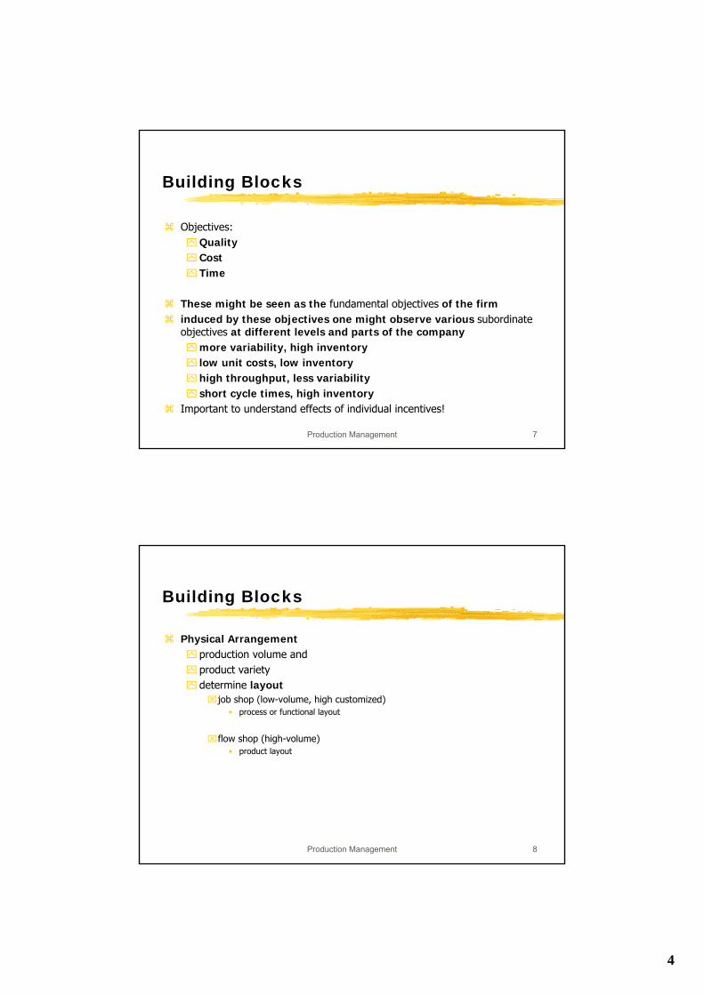
The PPC function integrates material flow using the information system. Integration is achieved through a common database.
DATABASE
ForecastingMaster
ProductionSchedule
ProductStructure
CustomerOrders
Purchasing& Receiving
Cost Quality Inventory
Engineering
Shop FloorControl
4
Production Management 7
Building Blocks
Objectives:QualityCostTime
These might be seen as the fundamental objectives of the firminduced by these objectives one might observe various subordinate objectives at different levels and parts of the company
more variability, high inventorylow unit costs, low inventoryhigh throughput, less variabilityshort cycle times, high inventory
Important to understand effects of individual incentives!
Production Management 8
Building Blocks
Physical Arrangement production volume andproduct varietydetermine layout⌧job shop (low-volume, high customized)
• process or functional layout
⌧flow shop (high-volume)• product layout
5
Production Management 9
Building Blocks
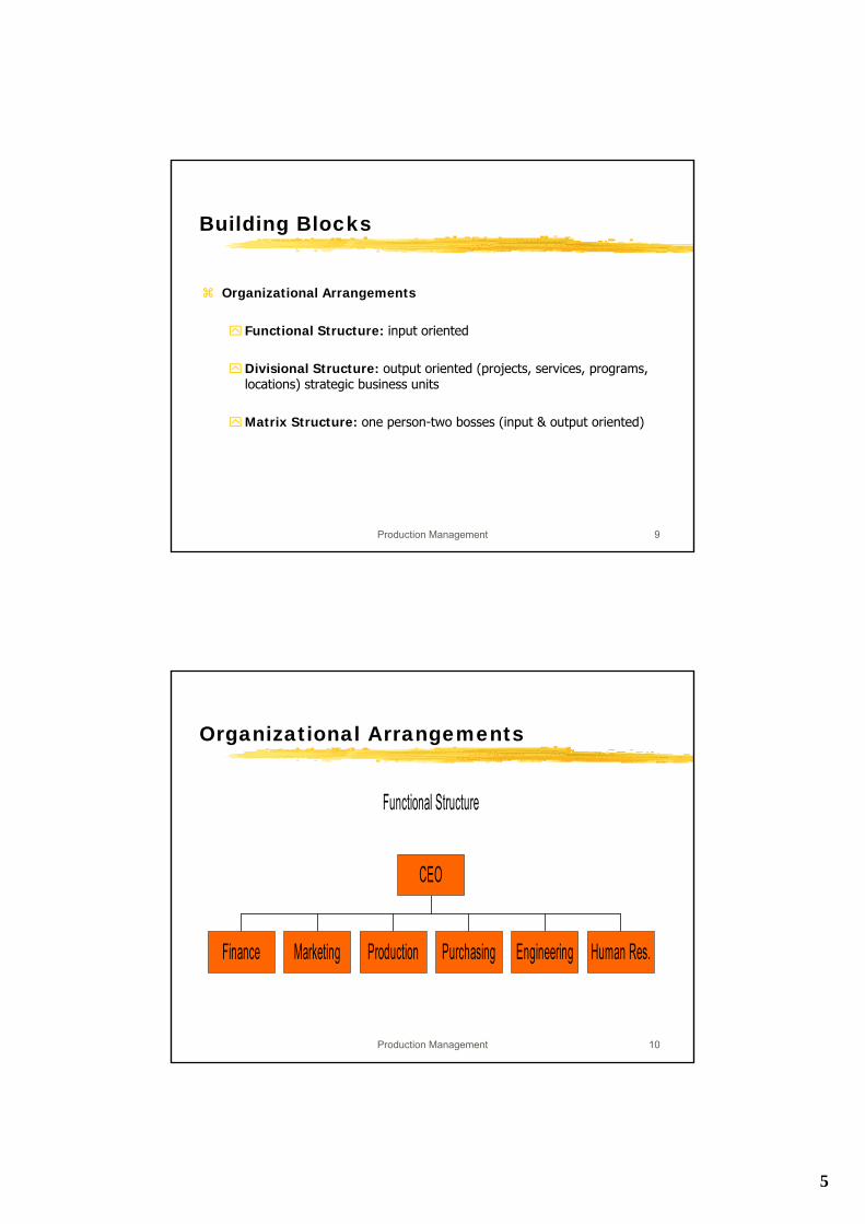
Organizational Arrangements
Functional Structure: input oriented
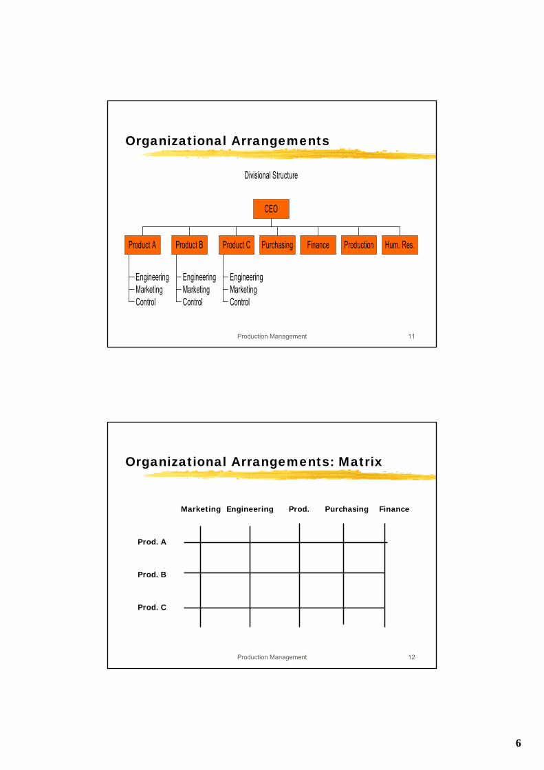
Divisional Structure: output oriented (projects, services, programs, locations) strategic business units
Matrix Structure: one person-two bosses (input & output oriented)
Production Management 10
Organizational Arrangements
Functional Structure
Finance Marketing Production Purchasing Engineering Human Res.
CEO
6
Production Management 11
Organizational Arrangements
Divisional Structure
EngineeringMarketingControl
Product A
EngineeringMarketingControl
Product B
EngineeringMarketingControl
Product C Purchasing Finance Production Hum. Res.
CEO
Production Management 12
Organizational Arrangements: Matrix
Marketing Engineering Prod. Purchasing Finance
Prod. A
Prod. B
Prod. C
7
Production Management 13
Production Planning and Control (PPC)
Intergrated-material-flow-based information system
based on a feedback loop (control theory)
management of deviations
art of selecting the appropriate mix of management technologies
impact of organizational structure, life-cycle effects
Production Management 14
Building Blocks
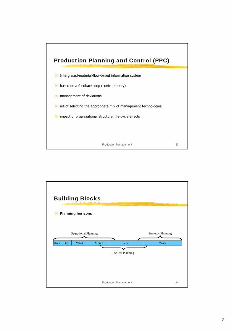
Planning horizons
Hour Day Week Month Year Years
Operational Planning Strategic Planning
Tactical Planning
8
Production Management 15
Building Blocks
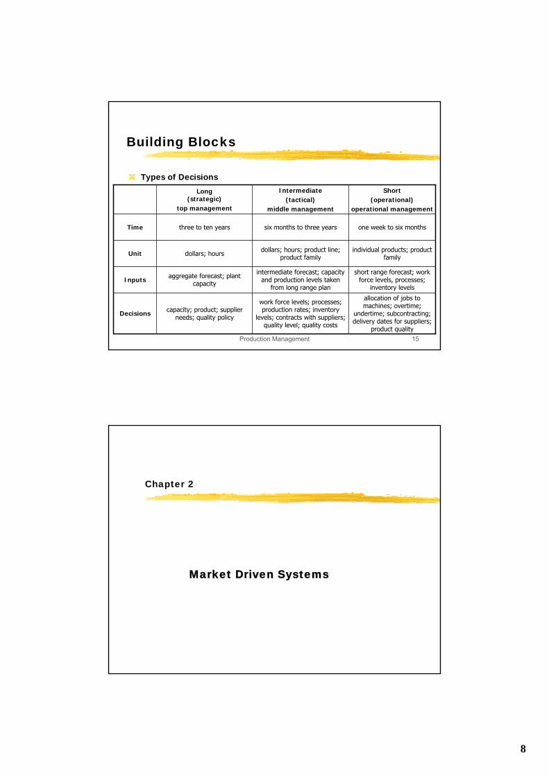
Types of Decisions
allocation of jobs to machines; overtime;
undertime; subcontracting; delivery dates for suppliers;
product quality
work force levels; processes; production rates; inventory
levels; contracts with suppliers; quality level; quality costs
capacity; product; supplier needs; quality policyDecisions
short range forecast; work force levels, processes;
inventory levels
intermediate forecast; capacity and production levels taken
from long range plan
aggregate forecast; plant capacityInputs
individual products; product family
dollars; hours; product line; product familydollars; hoursUnit
one week to six monthssix months to three yearsthree to ten yearsTime
Short(operational)
operational management
Intermediate(tactical)
middle management
Long(strategic)
top management
Chapter 2
Market Driven Systems
9
Production Management 17
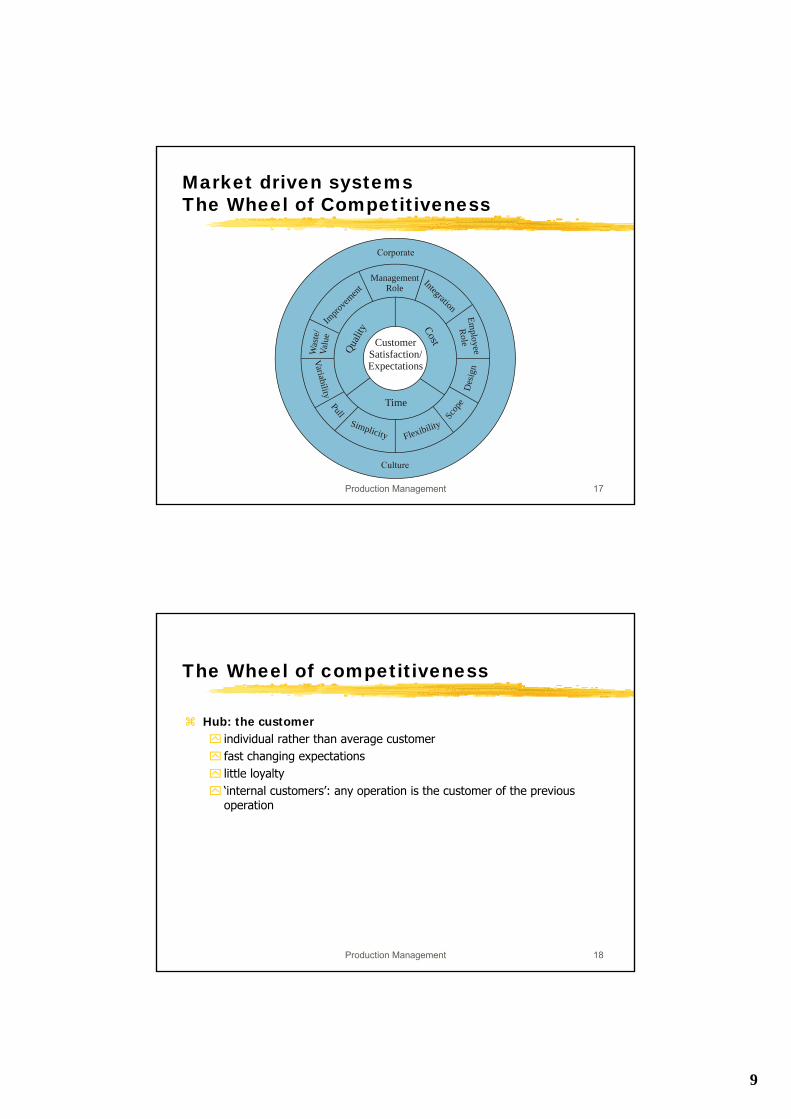
Market driven systemsThe Wheel of Competitiveness
CustomerSatisfaction/Expectations
Quali
ty Cost
Time
ManagementRole
IntegrationEm
ployeeR
ole
Des
ign
Scop
e
FlexibilitySimplicity
Pull
Variability
Was
te/
Valu
eIm
prove
ment
Production Management 18
The Wheel of competitiveness
Hub: the customerindividual rather than average customerfast changing expectationslittle loyalty‘internal customers’: any operation is the customer of the previous operation
10
Production Management 19
The Wheel of competitiveness
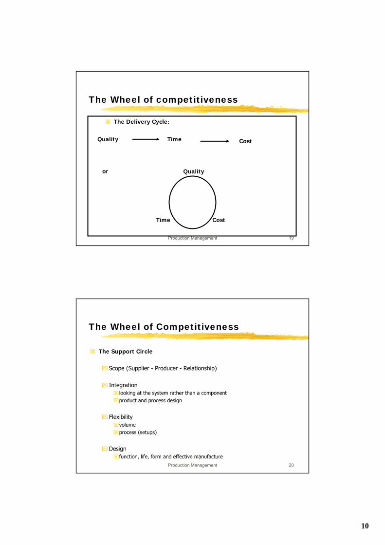
Quality Time Cost
The Delivery Cycle:
or Quality
CostTime
Production Management 20
The Wheel of Competitiveness
The Support Circle
Scope (Supplier - Producer - Relationship)
Integration ⌧looking at the system rather than a component⌧product and process design
Flexibility ⌧volume⌧process (setups)
Design⌧function, life, form and effective manufacture
11
Production Management 21
The Wheel of Competitiveness
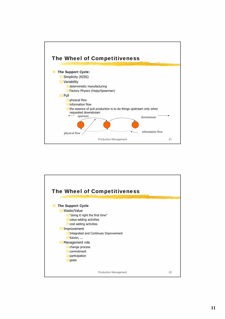
The Support Cycle:Simplicity (KISS)Variability⌧deterministic manufacturing⌧Factory Physics (Hopp/Spearman)
Pull⌧physical flow⌧information flow⌧the essence of pull production is to do things upstream only when
requested downstreamupstream downstream
information flowphysical flow
Production Management 22
The Wheel of Competitiveness
The Support CycleWaste/Value⌧“doing it right the first time”⌧value-adding activities⌧cost adding activities
Improvement⌧Integrated and Continues Improvement⌧Kaizen, ...
Management role⌧change process⌧commitment⌧participation⌧goals
12
Production Management 23
The Wheel of CompetitivenessThe Support Cycle
Employee role⌧involvement⌧development
The impact circleEfficiency: make things right⌧local⌧ration of output to input
Effectiveness: requirements of the total system
Production Management 24
Implementation
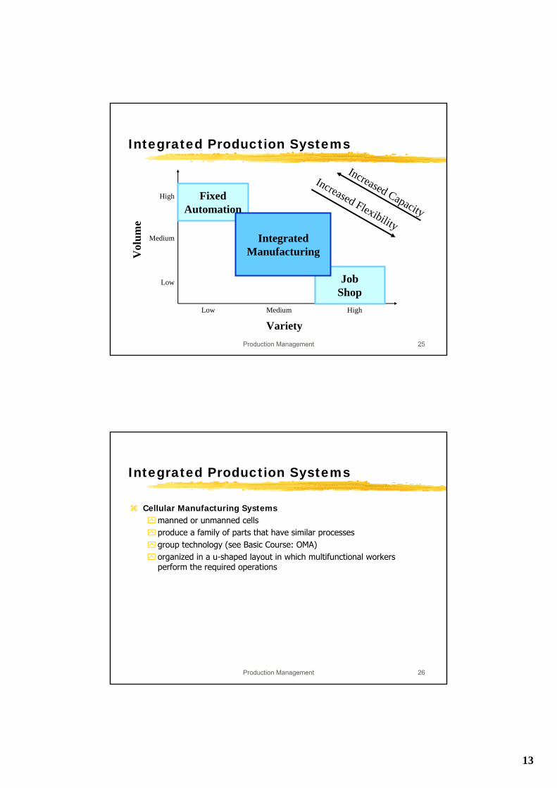
Integrated Production Systemsbest applied in the medium-variety, medium-volume rangeinformation integration is key aspect
3 leading approachesCellular Manufacturing Systems (CMS)Flexible Manufacturing Systems (FMS)Computer Integrated Manufacturing Systems (CIM)
13
Production Management 25
Integrated Production Systems
Low
Low Medium
Medium
High
High
Variety
Vol
ume
FixedAutomation
JobShop
IntegratedManufacturing
Increased Capacity
Increased Flexibility
Production Management 26
Integrated Production Systems
Cellular Manufacturing Systemsmanned or unmanned cellsproduce a family of parts that have similar processesgroup technology (see Basic Course: OMA)organized in a u-shaped layout in which multifunctional workers perform the required operations
14
Production Management 27
Integrated Production Systems
Flexible Manufacturing Systems integration of⌧manufacturing or assembly processes ⌧automated material flow systems ⌧computer communication⌧control
computer control system does:
⌧production control⌧scheduling⌧flow control⌧machine control
reaction to real time status dataautomotive and electronics industry
Production Management 28
Integrated Production Systems
Computer Integrated Manufacturing (CIM)broader scope than CMSuse information technology to coordinate business functions withproduct development, design and manufacturing‚bridges‘ between FMS islands
15
Production Management 29
Market driven systems
Integration Processteamworkconcurrent engineering⌧life cycle engineering⌧product and process design are considered together⌧cross functional teams
TQMWorld class manufacturingLean production(Toyota, production floor focus)Agile manufacturing(enterprise view)
Chapter 3
Problem Solving
16
Production Management 31
Problem Solving
Current state goal state
impact: should be worth the resource
ability to measure the gap
ability to close the gap
solve or dissolve
Production Management 32
Problem Solving
Problem IdentifikationSymptomsProblem missionmission will be translated into goals and objectivesproblem owners: people who must live with the solutionAssumptionsInitial Problem Statement
17
Production Management 33
Problem Solving
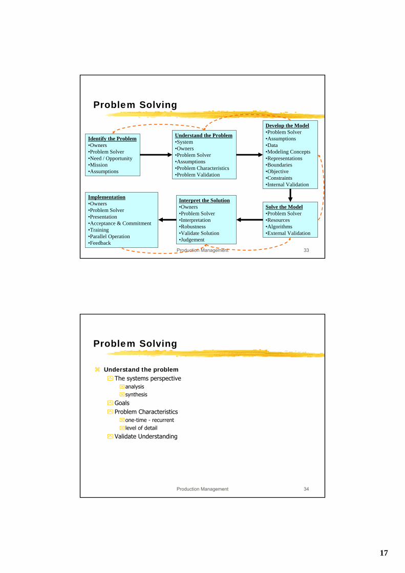
Identify the Problem•Owners•Problem Solver•Need / Opportunity•Mission•Assumptions
Understand the Problem•System•Owners•Problem Solver•Assumptions•Problem Characteristics•Problem Validation
Develop the Model•Problem Solver•Assumptions•Data•Modeling Concepts•Representations•Boundaries•Objective•Constraints•Internal Validation
Solve the Model•Problem Solver•Resources•Algorithms•External Validation
Interpret the Solution•Owners•Problem Solver•Interpretation•Robustness•Validate Solution•Judgement
Implementation•Owners•Problem Solver•Presentation•Acceptance & Commitment•Training•Parallel Operation•Feedback
Production Management 34
Problem Solving
Understand the problemThe systems perspective⌧analysis⌧synthesis
GoalsProblem Characteristics⌧one-time - recurrent⌧level of detail
Validate Understanding
18
Production Management 35
Problem Solving
Develop a modelModel representation⌧iconic⌧analog⌧symbolic
DataModeling concepts⌧Boundaries⌧Objectives⌧Constraints
RelationshipsAssumptions and InvolvementInternal validation
Production Management 36
Problem Solving
Solve the ModelExternal validationSimplificationSolution Strategy⌧Exact⌧Heuristic⌧Simulation
Interpret the solutionrobustnessplausibility
Implementation
19
Production Management 37
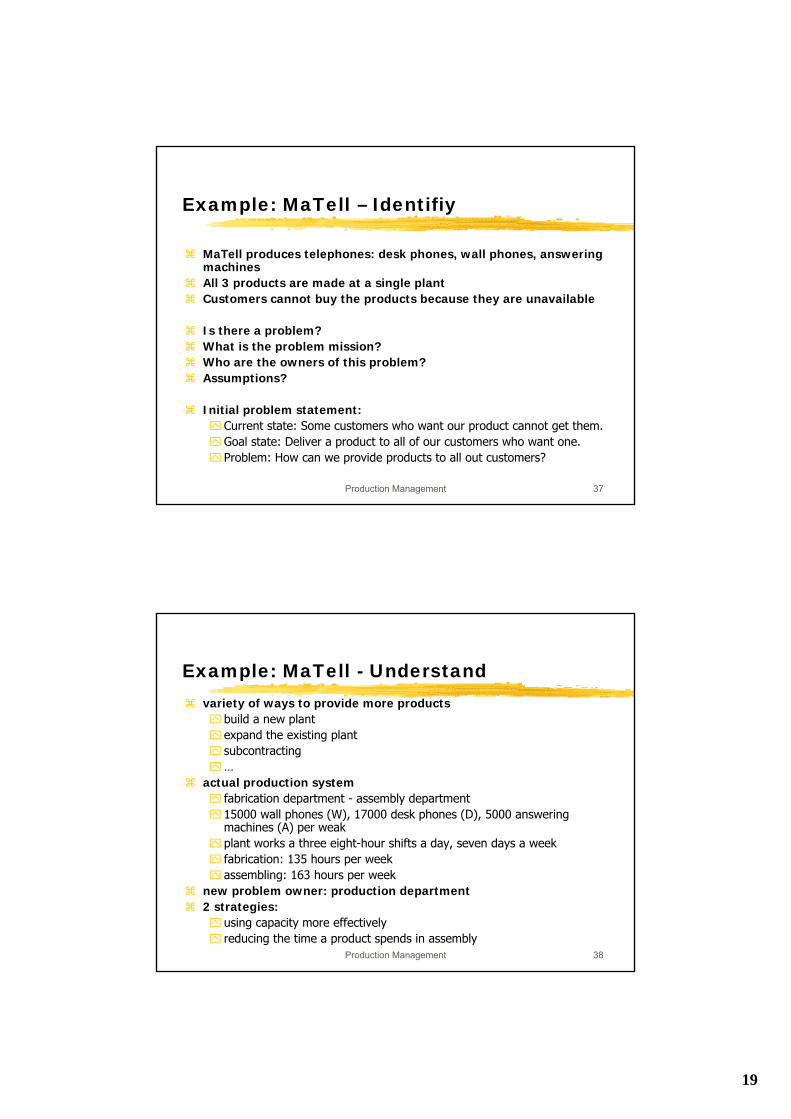
Example: MaTell – Identifiy
MaTell produces telephones: desk phones, wall phones, answering machinesAll 3 products are made at a single plantCustomers cannot buy the products because they are unavailable
Is there a problem?What is the problem mission?Who are the owners of this problem?Assumptions?
Initial problem statement:Current state: Some customers who want our product cannot get them.Goal state: Deliver a product to all of our customers who want one.Problem: How can we provide products to all out customers?
Production Management 38
Example: MaTell - Understandvariety of ways to provide more products
build a new plantexpand the existing plantsubcontracting…
actual production systemfabrication department - assembly department15000 wall phones (W), 17000 desk phones (D), 5000 answering machines (A) per weakplant works a three eight-hour shifts a day, seven days a weekfabrication: 135 hours per weekassembling: 163 hours per week
new problem owner: production department2 strategies:
using capacity more effectivelyreducing the time a product spends in assembly
20
Production Management 39
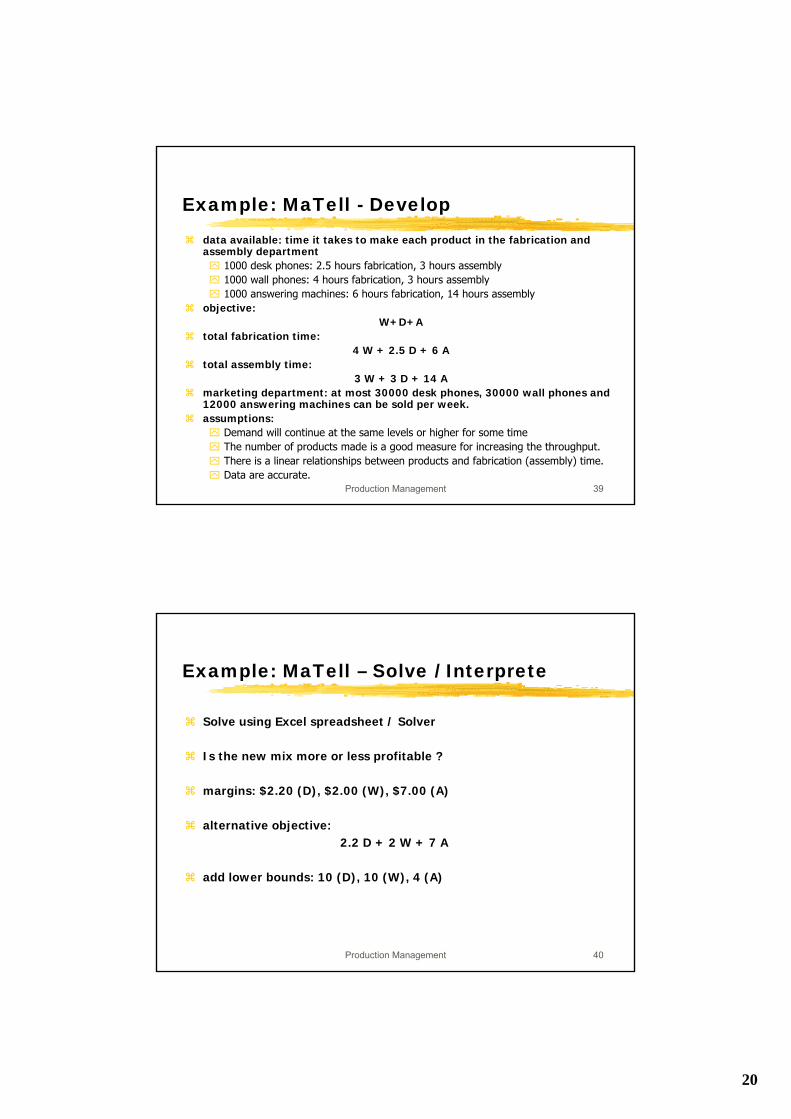
Example: MaTell - Develop
data available: time it takes to make each product in the fabrication and assembly department
1000 desk phones: 2.5 hours fabrication, 3 hours assembly1000 wall phones: 4 hours fabrication, 3 hours assembly1000 answering machines: 6 hours fabrication, 14 hours assembly
objective:W+D+A
total fabrication time:4 W + 2.5 D + 6 A
total assembly time:3 W + 3 D + 14 A
marketing department: at most 30000 desk phones, 30000 wall phones and 12000 answering machines can be sold per week.assumptions:
Demand will continue at the same levels or higher for some timeThe number of products made is a good measure for increasing the throughput.There is a linear relationships between products and fabrication (assembly) time.Data are accurate.
Production Management 40
Example: MaTell – Solve / Interprete
Solve using Excel spreadsheet / Solver
Is the new mix more or less profitable ?
margins: $2.20 (D), $2.00 (W), $7.00 (A)
alternative objective:2.2 D + 2 W + 7 A
add lower bounds: 10 (D), 10 (W), 4 (A)
21
Production Management 41
Example: MaTell – Implementation
present the solutionThough the spreadsheet was not used to get the solution, it would be a good way to introduce the LP solution
acceptance relatively easy (owners were involved)
commitment may be more difficult, but only few resources needed (LP package, training for the planner)
check the system from time to time (conditions may change)
Production Management 42
Problem Solving
Work to do:
Examples: 3.12 abcd, 3.19 ab, 3.30abc, 3.36abc, 3.41 abc, 3.46
22
Chapter 5
Aggregate Planning
Production Management 44
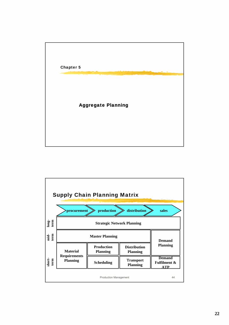
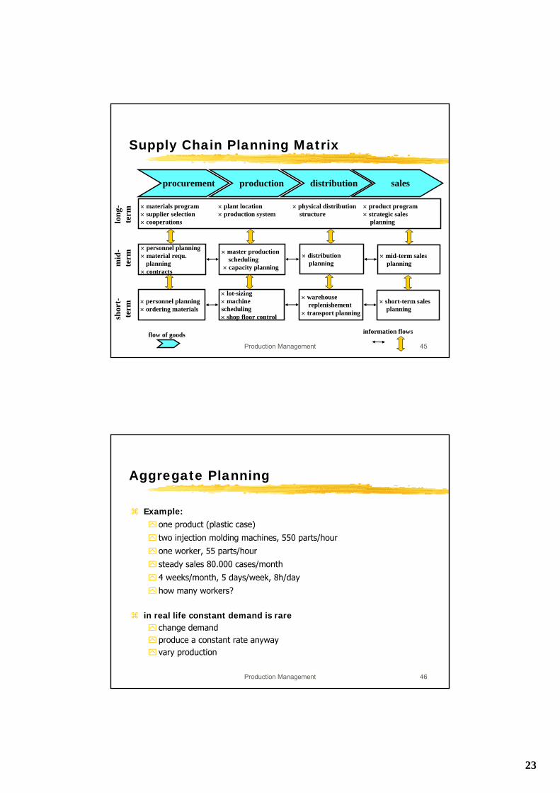
Supply Chain Planning Matrix
production distribution salesprocurement
Strategic Network Planning
Master Planning
Distribution Planning
Transport Planning
ProductionPlanning
DemandPlanning
DemandFulfilment &
ATPScheduling
Material Requirements
Planning
long
-te
rmm
id-
term
shor
t-te
rm
23
Production Management 45
Supply Chain Planning Matrix
production distribution salesprocurement
× materials program × plant location × physical distribution × product program× supplier selection × production system structure × strategic sales× cooperations planning
× personnel planning× material requ.
planning× contracts
× mid-term salesplanning
long
-te
rmm
id-
term
shor
t-te
rm
× master productionscheduling
× capacity planning
× distributionplanning
× personnel planning× ordering materials
× short-term salesplanning
× lot-sizing× machinescheduling× shop floor control
× warehousereplenishement
× transport planning
information flowsflow of goods
Production Management 46
Aggregate Planning
Example:one product (plastic case)
two injection molding machines, 550 parts/hour
one worker, 55 parts/hour
steady sales 80.000 cases/month
4 weeks/month, 5 days/week, 8h/day
how many workers?
in real life constant demand is rarechange demandproduce a constant rate anywayvary production
24
Production Management 47
Aggregate Planning
Influencing demanddo not satisfy demandshift demand from peak periods to nonpeak periodsproduce several products with peak demand in different period
Planning ProductionProduction plan: how much and when to make each productrolling planning horizonlong range planintermediate-range plan⌧units of measurements are aggregates⌧product family⌧plant department⌧changes in workforce, additional machines, subcontracting, overtime,...
Short-term plan
Production Management 48
Aggregate Planning
Aspects of Aggregate PlanningCapacity: how much a production system can makeAggregate Units: products, workers,...Costs⌧production costs (economic costs!)⌧inventory costs(holding and shortage)⌧capacity change costs
25
Production Management 49
Aggregate Planning
Spreadsheet MethodsZero Inventory Plan
Precision Transfer, Inc. Produces more than 300 different precision gears ( the aggregation unit is a gear!). Last year (=260 working days) Precision made 41.383 gears of various kinds with an average of 40 workers.41.383 gears per year40 x 260 worker-days/year = 3,98 -> 4 gears/ worker-day
Aggregate demand forecast for precision gear:
Month January February March April May June TotalDemand 2760 3320 3970 3540 3180 2900 19.670
Production Management 50
Aggregate Planning
holding costs: $5 per gear per monthbacklog costs: $15 per gear per monthhiring costs: $450 per workerlay-off costs: $600 per workerwages: $15 per hour ( all workers are paid for 8 hours per day)there are currently 35 workers at Precisioncurrently no inventory
Production plan?
26
Production Management 51
Aggregate Planning
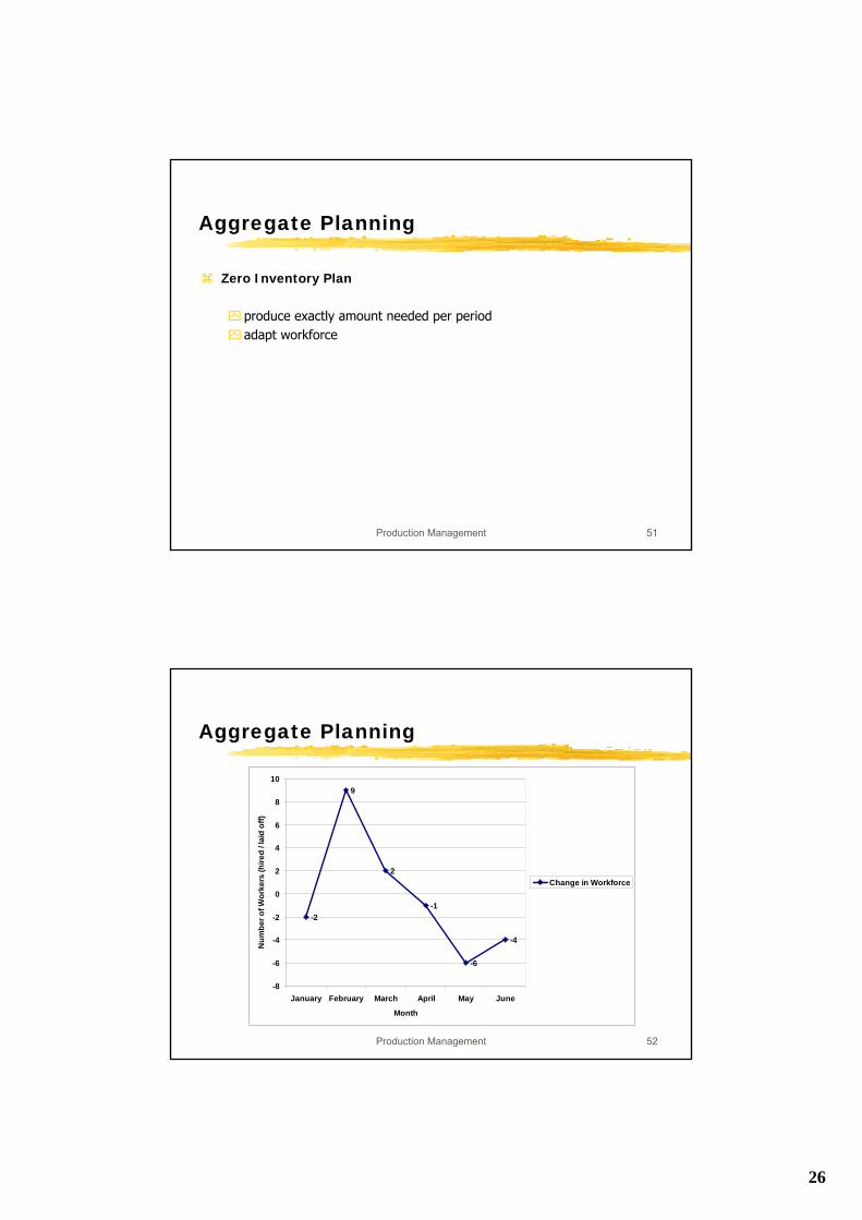
Zero Inventory Plan
produce exactly amount needed per periodadapt workforce
Production Management 52
Aggregate Planning
-2
9
2
-1
-6
-4
-8
-6
-4
-2
0
2
4
6
8
10
January February March April May June
Month
Num
ber o
f Wor
kers
(hire
d / l
aid
off)
Change in Workforce
27
Production Management 53
Aggregate Planning
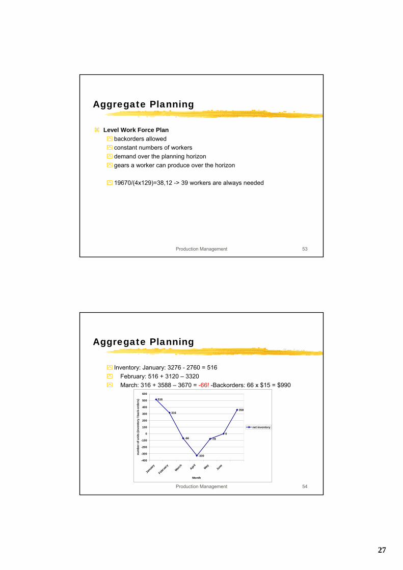
Level Work Force Planbackorders allowedconstant numbers of workersdemand over the planning horizongears a worker can produce over the horizon
19670/(4x129)=38,12 -> 39 workers are always needed
Production Management 54
Aggregate Planning
Inventory: January: 3276 - 2760 = 516February: 516 + 3120 – 3320March: 316 + 3588 – 3670 = -66! -Backorders: 66 x $15 = $990
516
316
-66
-330
-78
0
358
-400
-300
-200
-100
0
100
200
300
400
500
600
Janua
ry
Febru
ary
March
April
MayJu
ne
Month
num
ber o
f uni
ts (i
nven
tory
/ ba
ck-o
rder
s)
net inventory
28
Production Management 55
Aggregate Planning
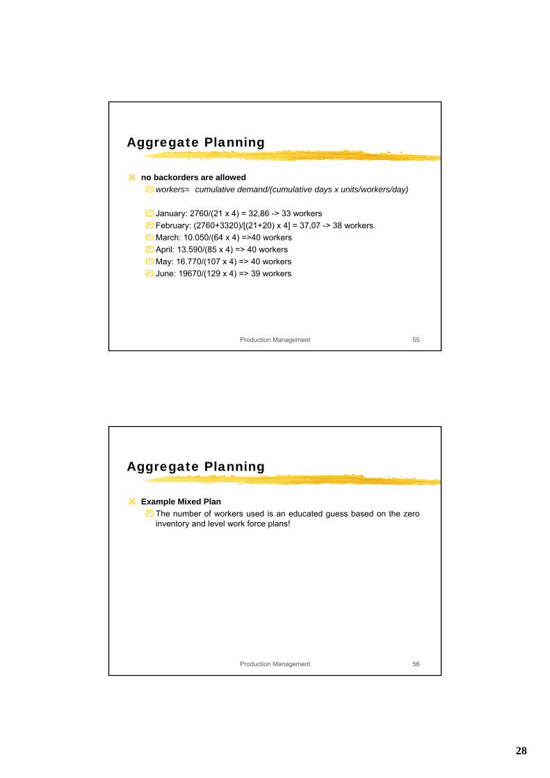
no backorders are allowedworkers= cumulative demand/(cumulative days x units/workers/day)
January: 2760/(21 x 4) = 32,86 -> 33 workersFebruary: (2760+3320)/[(21+20) x 4] = 37,07 -> 38 workers.March: 10.050/(64 x 4) =>40 workersApril: 13.590/(85 x 4) => 40 workersMay: 16.770/(107 x 4) => 40 workersJune: 19670/(129 x 4) => 39 workers
Production Management 56
Aggregate Planning
Example Mixed PlanThe number of workers used is an educated guess based on the zero inventory and level work force plans!
29
Production Management 57
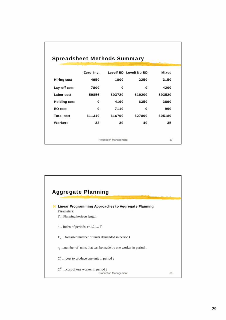
Spreadsheet Methods Summary
Zero-Inv. Level/BO Level/No BO Mixed
Hiring cost 4950 1800 2250 3150
Lay-off cost 7800 0 0 4200
Labor cost 59856 603720 619200 593520
Holding cost 0 4160 6350 3890
BO cost 0 7110 0 990
Total cost 611310 616790 627800 605180
Workers 33 39 40 35
Production Management 58
Aggregate Planning
Linear Programming Approaches to Aggregate PlanningParameters:T... Planning horizon length
t ... Index of periods, t=1,2,..., T
forcasted number of units demanded in period t
number of units that can be made by one worker in period t
cost to pr
t
t
Pt
D
n
C
K
K
K oduce one unit in period t
cost of one worker in period tWtC K
30
Production Management 59
Aggregate Planning
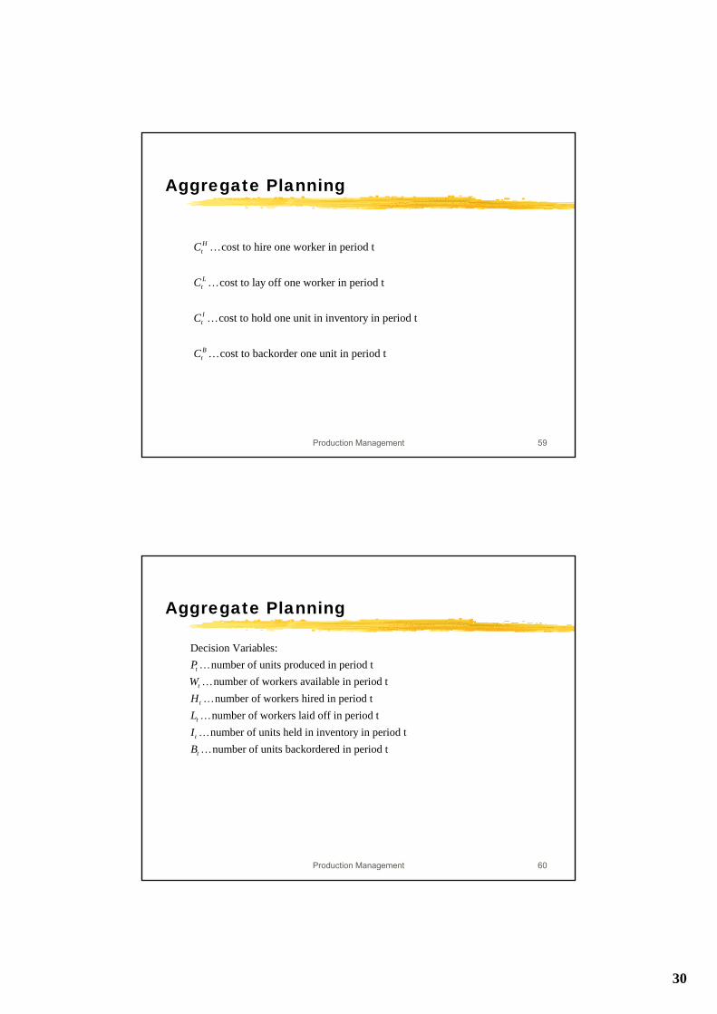
cost to hire one worker in period t
cost to lay off one worker in period t
cost to hold one unit in inventory in period t
cost to backorder one unit in period t
Ht
Lt
It
Bt
C
C
C
C
K
K
K
K
Production Management 60
Aggregate Planning
Decision Variables:number of units produced in period tnumber of workers available in period tnumber of workers hired in period t
number of workers laid off in period tnumber of units he
t
t
t
t
t
PWHLI
K
K
K
K
K ld in inventory in period tnumber of units backordered in period ttB K
31
Production Management 61
Aggregate Planning
t
t 1
Constraints: work, Capacity, force, materialP 1,2,...,W 1, 2,...,
net inventory this period = net inventory last period + productio
t t
t t t
nW t TW H L t T−
≤ == + − =
t t-1 1
TP W H L I Bt t t t t t t t t t t t
t=1
n this period - demand this periodI I
Costs
(C P +C W +C H +C L +C I +C B )
t t t tB B P D−− = − + −
∑
Production Management 62
Aggregate Planning
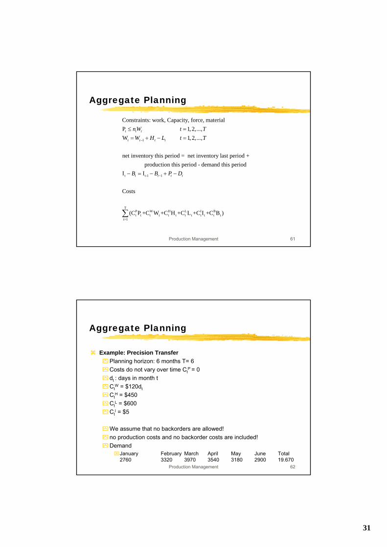
Example: Precision TransferPlanning horizon: 6 months T= 6Costs do not vary over time Ct
P = 0dt : days in month tCt
W = $120dt
CtH = $450
CtL = $600
CtI = $5
We assume that no backorders are allowed!no production costs and no backorder costs are included!Demand⌧January February March April May June Total
2760 3320 3970 3540 3180 2900 19.670
32
Production Management 63
Linear Program Model for PrecisionTransfer
Production Management 64
Aggregate Planning
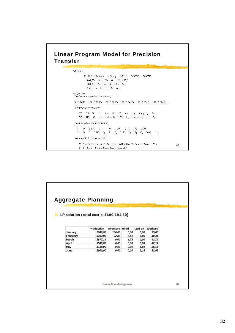
LP solution (total cost = $600 191,60)
Production Inventory Hired Laid off WorkersJanuary 2940,00 180,00 0,00 0,00 35,00February 3232,86 92,86 5,41 0,00 40,41March 3877,14 0,00 1,73 0,00 42,14April 3540,00 0,00 0,00 0,00 42,14May 3180,00 0,00 0,00 6,01 36,14June 2900,00 0,00 0,00 3,18 32,95
33
Production Management 65
Aggregate Planning
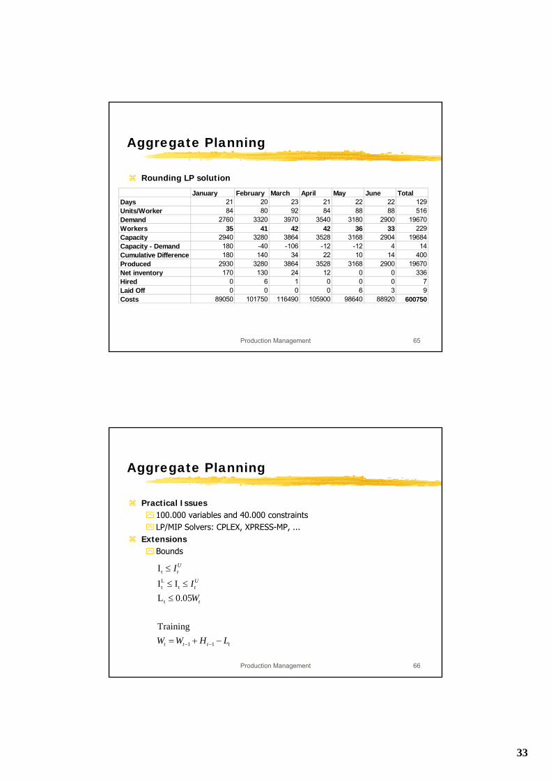
Rounding LP solution
January February March April May June TotalDays 21 20 23 21 22 22 129Units/Worker 84 80 92 84 88 88 516Demand 2760 3320 3970 3540 3180 2900 19670Workers 35 41 42 42 36 33 229Capacity 2940 3280 3864 3528 3168 2904 19684Capacity - Demand 180 -40 -106 -12 -12 4 14Cumulative Difference 180 140 34 22 10 14 400Produced 2930 3280 3864 3528 3168 2900 19670Net inventory 170 130 24 12 0 0 336Hired 0 6 1 0 0 0 7Laid Off 0 0 0 0 6 3 9Costs 89050 101750 116490 105900 98640 88920 600750
Production Management 66
Aggregate Planning
Practical Issues100.000 variables and 40.000 constraintsLP/MIP Solvers: CPLEX, XPRESS-MP, ...
ExtensionsBounds
t
Lt t
t
1 1
I
I IL 0.05
Training
Ut
Ut
t
t t t t
I
IW
W W H L− −
≤
≤ ≤≤
= + −
34
Production Management 67
Aggregate Planning
Transportation Modelssupply points: periods, initial inventorydemand points: periods, excess demand, final inventory
PtIt
capacity during period tforecasted number of units demanded in period t
C the cost to produce one unit in period t
C the cost to hold one unit in inventory in period t
t t
t
nWD
==
=
=
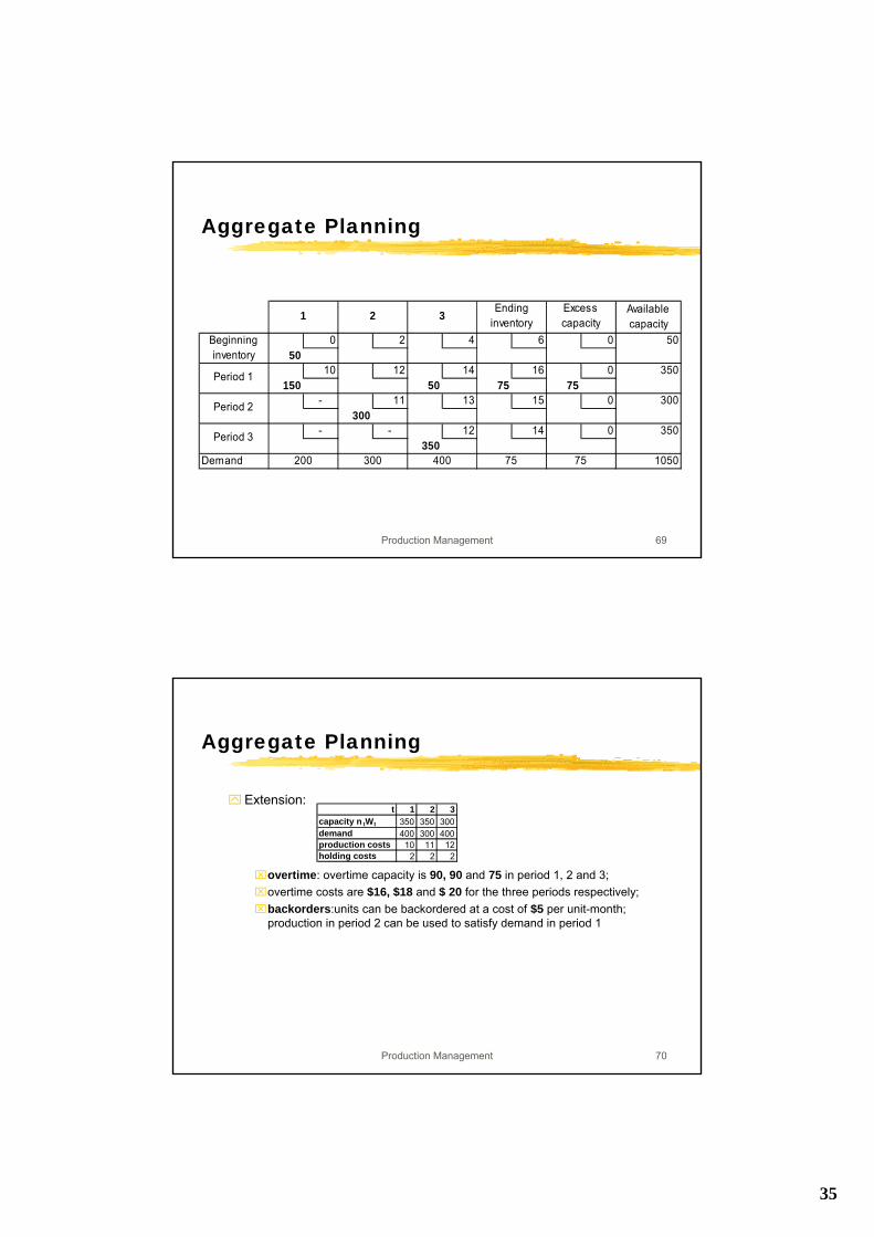
Production Management 68
Aggregate Planning
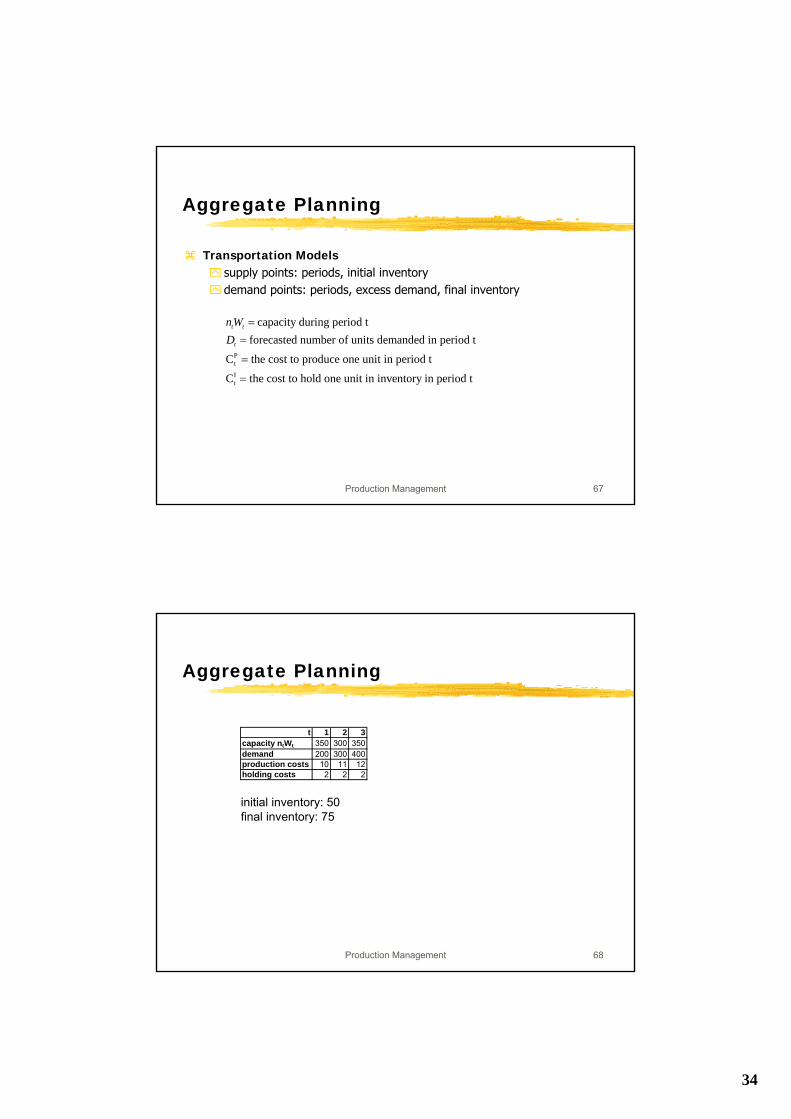
t 1 2 3capacity ntWt 350 300 350demand 200 300 400production costs 10 11 12holding costs 2 2 2
initial inventory: 50final inventory: 75
35
Production Management 69
Aggregate Planning
Availablecapacity
0 2 4 6 0 5050
10 12 14 16 0 350150 50 75 75
- 11 13 15 0 300300
- - 12 14 0 350350
Demand 1050
Excess capacity
Ending inventory1 2 3
Beginning inventory
Period 1
Period 2
Period 3
75200 300 400 75
Production Management 70
Aggregate Planning
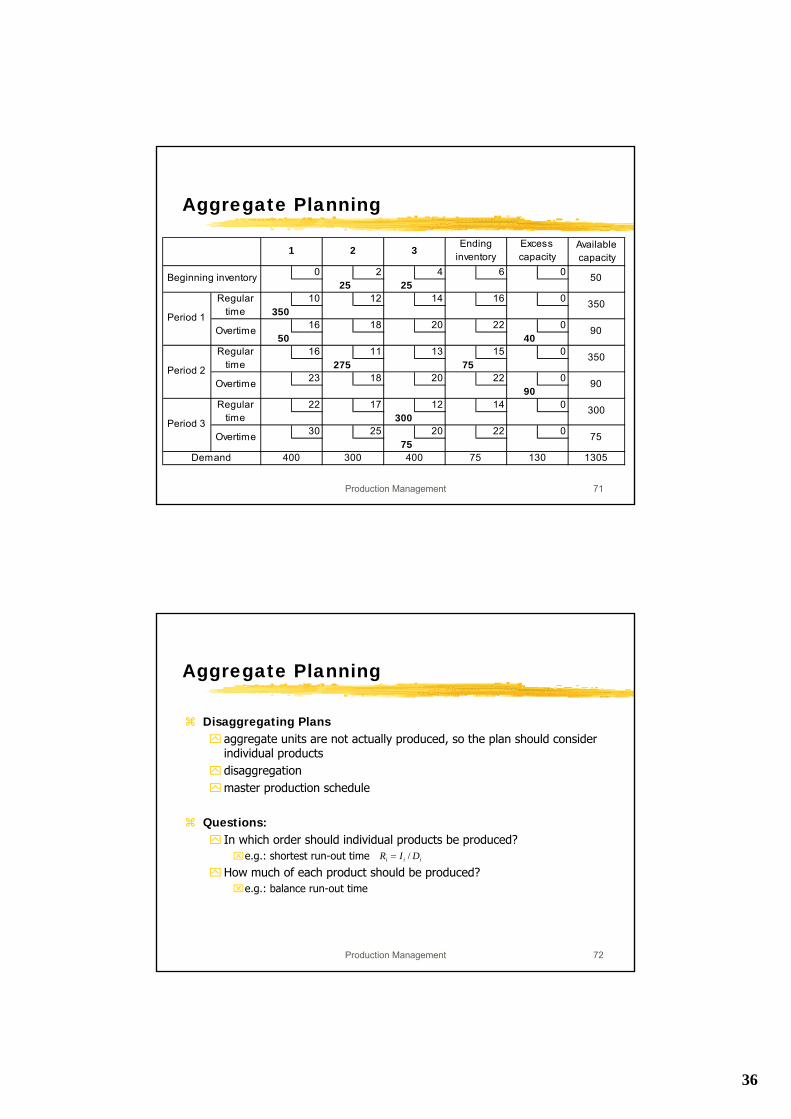
Extension:
⌧overtime: overtime capacity is 90, 90 and 75 in period 1, 2 and 3;⌧overtime costs are $16, $18 and $ 20 for the three periods respectively;⌧backorders:units can be backordered at a cost of $5 per unit-month;
production in period 2 can be used to satisfy demand in period 1
t 1 2 3capacity n tWt 350 350 300demand 400 300 400production costs 10 11 12holding costs 2 2 2
36
Production Management 71
Aggregate Planning
Availablecapacity
0 2 4 6 025 25
10 12 14 16 0350
16 18 20 22 050 40
16 11 13 15 0275 75
23 18 20 22 090
22 17 12 14 0300
30 25 20 22 075
1305Demand
Excess capacity
Ending inventory1 2 3
130400 300 400 75
Beginning inventory
Period 1
Regular time
Overtime
Regular time
Overtime
Period 3
Regular time
Overtime
Period 2
90
350
50
75
300
90
350
Production Management 72
Aggregate Planning
Disaggregating Plansaggregate units are not actually produced, so the plan should consider individual productsdisaggregationmaster production schedule
Questions:In which order should individual products be produced?⌧e.g.: shortest run-out time
How much of each product should be produced?⌧e.g.: balance run-out time
iii DIR /=
37
Production Management 73
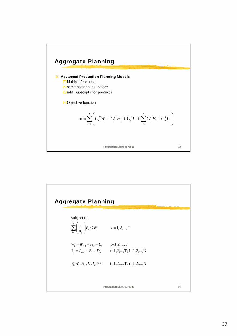
Aggregate Planning
Advanced Production Planning ModelsMultiple Productssame notation as beforeadd subscript i for product i
Objective function
∑ ∑= =
⎟⎠
⎞⎜⎝
⎛++++
T
t
N
iit
Iitit
Pitt
Ltt
Htt
Wt ICPCLCHCWC
1 1
min
Production Management 74
Aggregate Planning
N
i=1
1
it 1
it,
subject to
1 1,2,...,
t=1,2,...,TI t=1,2,...,T; i=1,2,...,N
P , , , 0 t=1,2,...,T; i=1,2,...,N
it tit
t t t t
it it it
t t t it
P W t Tn
W W H LI P D
W H L I
−
−
⎛ ⎞≤ =⎜ ⎟
⎝ ⎠
= + −= + −
≥
∑
38
Production Management 75
Aggregate Planning
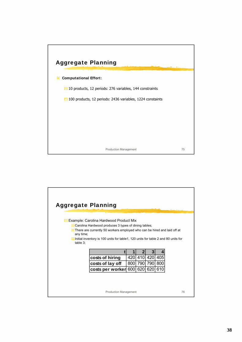
Computational Effort:
10 products, 12 periods: 276 variables, 144 constraints
100 products, 12 periods: 2436 variables, 1224 constaints
Production Management 76
Aggregate Planning
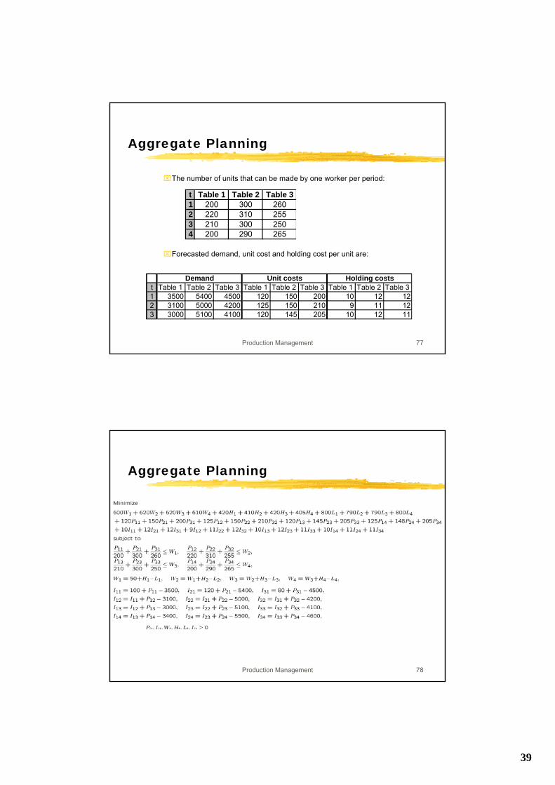
Example: Carolina Hardwood Product Mix⌧Carolina Hardwood produces 3 types of dining tables; ⌧There are currently 50 workers employed who can be hired and laid off at
any time;⌧Initial inventory is 100 units for table1, 120 units for table 2 and 80 units for
table 3;
t 1 2 3 4costs of hiring 420 410 420 405costs of lay off 800 790 790 800costs per worker 600 620 620 610
39
Production Management 77
Aggregate Planning
⌧The number of units that can be made by one worker per period:
⌧Forecasted demand, unit cost and holding cost per unit are:
t Table 1 Table 2 Table 31 200 300 2602 220 310 2553 210 300 2504 200 290 265
t Table 1 Table 2 Table 3 Table 1 Table 2 Table 3 Table 1 Table 2 Table 31 3500 5400 4500 120 150 200 10 12 122 3100 5000 4200 125 150 210 9 11 123 3000 5100 4100 120 145 205 10 12 11
Demand Unit costs Holding costs
Production Management 78
Aggregate Planning
40
Production Management 79
Aggregate Planning
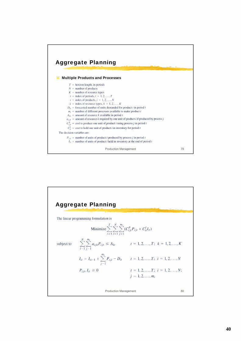
Multiple Products and Processes
Production Management 80
Aggregate Planning
41
Production Management 81
Aggregate Planning
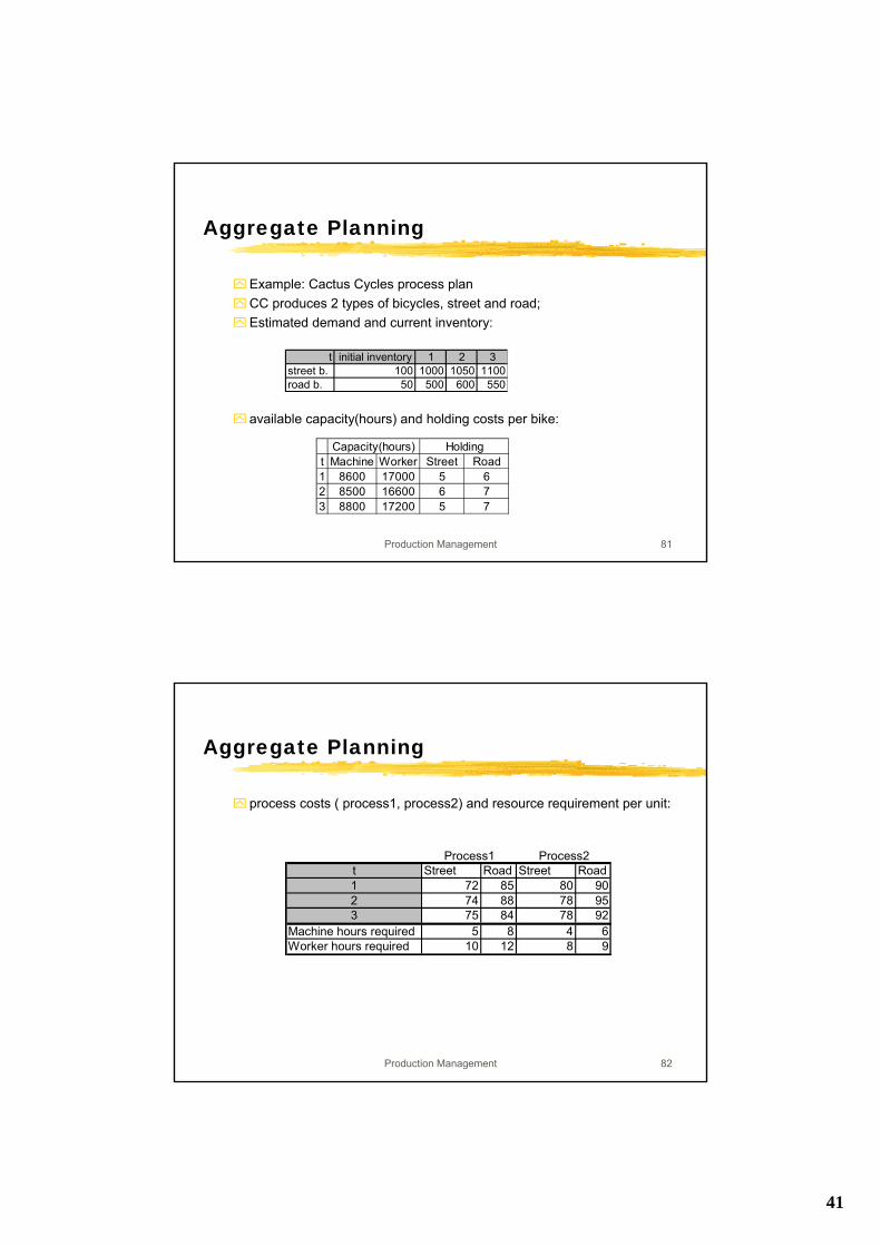
Example: Cactus Cycles process planCC produces 2 types of bicycles, street and road;Estimated demand and current inventory:
available capacity(hours) and holding costs per bike:
t initial inventory 1 2 3street b. 100 1000 1050 1100road b. 50 500 600 550
t Machine Worker Street Road1 8600 17000 5 62 8500 16600 6 73 8800 17200 5 7
Capacity(hours) Holding
Production Management 82
Aggregate Planning
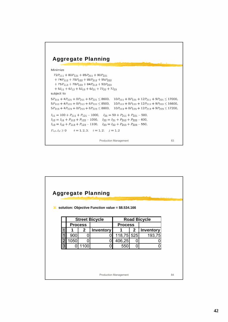
process costs ( process1, process2) and resource requirement per unit:
t Street Road Street Road1 72 85 80 902 74 88 78 953 75 84 78 92
Machine hours required 5 8 4 6Worker hours required 10 12 8 9
Process1 Process2
42
Production Management 83
Aggregate Planning
Production Management 84
Aggregate Planning
solution: Objective Function value = $8.534.166
t 1 2 Inventory 1 2 Inventory1 900 0 0 118,75 525 193,752 1050 0 0 406,25 0 03 0 1100 0 550 0 0
Process ProcessStreet Bicycle Road Bicycle
43
Production Management 85
Aggregate Planning - Extensions
Hopp/Spearman, S. 522-540Notation:
tperiodin produced iproduct ofamount ...Xit
)a t with(consisten units in t period in j on workstatiofcapacity ciproduct ofunit one produce toj on workstation required timea
tperiod in sold iproduct ofamount product ofunit one fromprofit net r
ijjt
ij
i
K
K
K
K
itSi
Production Management 86
Aggregate Planning - Extensions
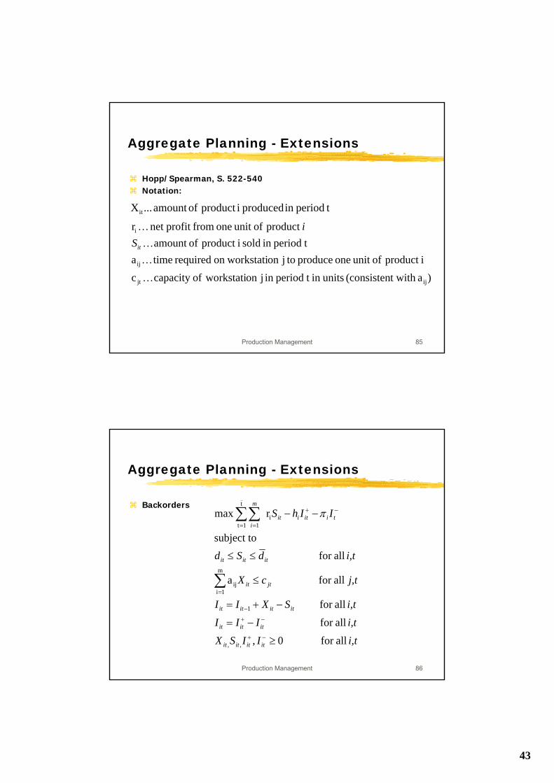
Backorders
i,tIISX
i,tIII
i,tSXII
j,tcX
i,tdSd
IIhS
itititit
ititit
itititit
jtit
ititit
tiitiit
m
i
allfor 0,
allfor
allfor
allfor a
allfor subject to
r max
,,
1
m
1iij
t
1ti
1
≥
−=
−+=
≤
≤≤
−−
−+
−+
−
=
−
=
+
=
∑
∑∑ π
44
Production Management 87
Aggregate Planning - Extensions
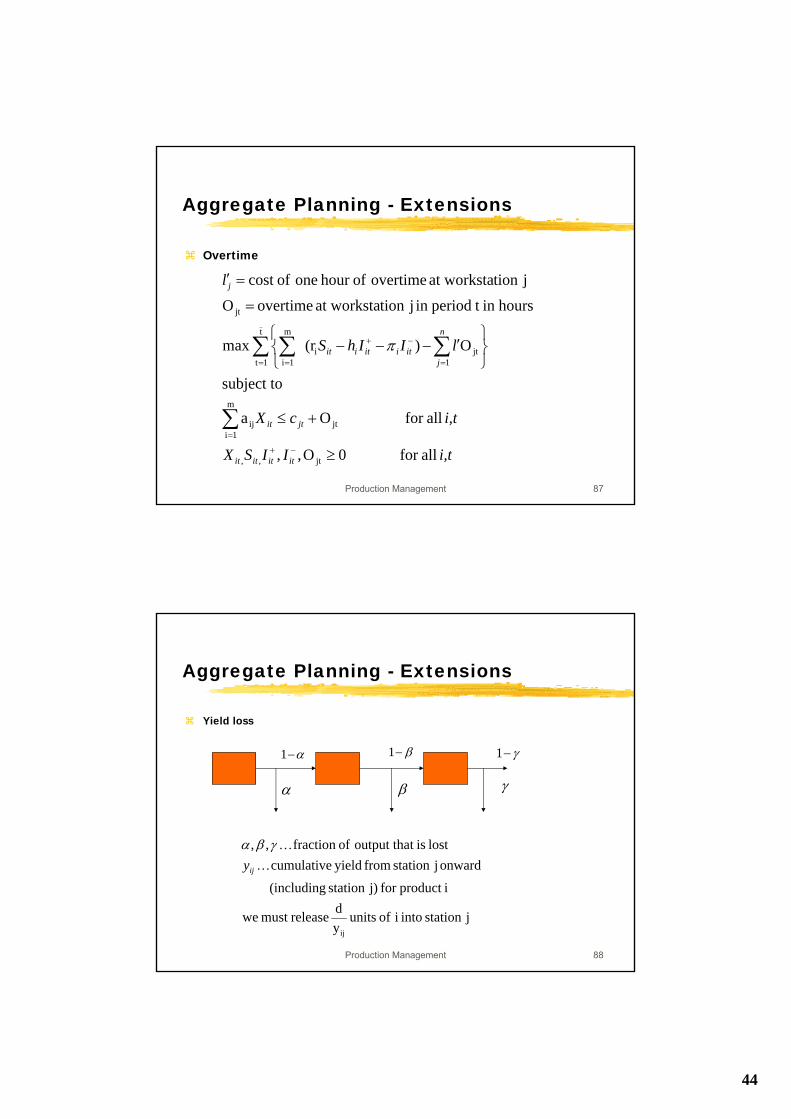
Overtime
i,tIISX
i,tcX
lIIhS
l
itititit
jtit
n
jitiitiit
j
allfor 0O,,
allfor Oa
subject to
O)(r max
hoursin t periodin jtion at worksta overtime Ojtion at worksta overtime ofhour one ofcost
jt,,
m
1ijtij
t
1t 1jti
m
1i
jt
≥
+≤
⎭⎬⎫
⎩⎨⎧
′−−−
=
=′
−+
=
= =
−+
=
∑
∑ ∑∑ π
Production Management 88
Aggregate Planning - Extensions
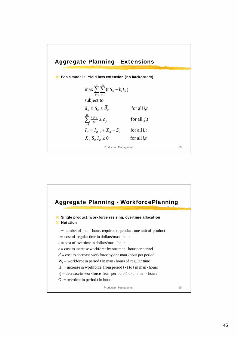
Yield loss
jstation into i of units yd releasemust we
iproduct for j)station (including
onward jstation from yield cumulativelost ist output tha offraction ,,
ij
K
K
ijyγβα
α−1 β−1
β
γ−1
γα
45
Production Management 89
Aggregate Planning - Extensions
Basic model + Yield loss extension (no backorders)
i,tISX
i,tSXII
j,tc
i,tdSd
IhS
ititit
itititit
jtyX
ititit
itiit
ij
it
allfor 0
allfor
allfor
allfor subject to
)r( max
,,
1
m
1i
a
t
1ti
m
1i
ij
≥
−+=
≤
≤≤
−
−
=
= =
∑
∑∑
Production Management 90
Aggregate Planning - WorkforcePlanning
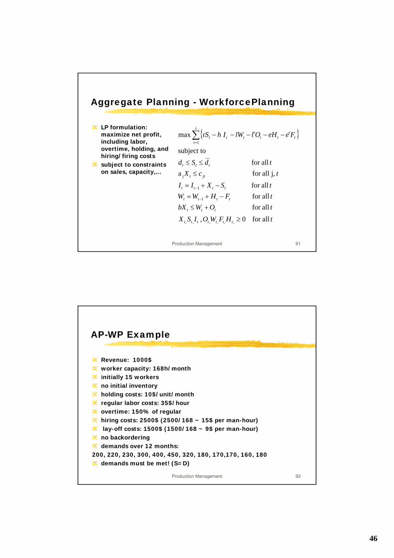
Single product, workforce resizing, overtime allocationNotation
hoursin t periodin overtimeOhours-manin t to1- tperiod from cein workfor decreaseFhours-manin t to1- tperiod from cein workfor increaseH
meregular ti of hours-manin t periodin workforceWperiodper hour -man oneby workforcedecrease cost toe
periodper hour -man oneby workforceincrease cost toehour -ndollars/main overtime ofcost
hour-ndollars/main meregular ti ofcost lproduct ofunit one produce torequired hours-man ofnumber b
t
t
t
t
====
=′==′==
l
46
Production Management 91
Aggregate Planning - WorkforcePlanning
LP formulation: maximize net profit, including labor, overtime, holding, and hiring/firing costssubject to constraints on sales, capacity,...
{ }
tHFWOISX
tOWbXtFHWWtSXII
tcXtdSd
FeeHOllWIhS
ttttttt
ttt
tttt
tttt
jtt
ttt
tttttt
allfor 0,
allfor allfor allfor
j, allfor a allfor
subject to
r max
,,,,,,
1
1
j
t
1t
≥
+≤−+=
−+=
≤≤≤
′−−′−−−
−
−
=∑
Production Management 92
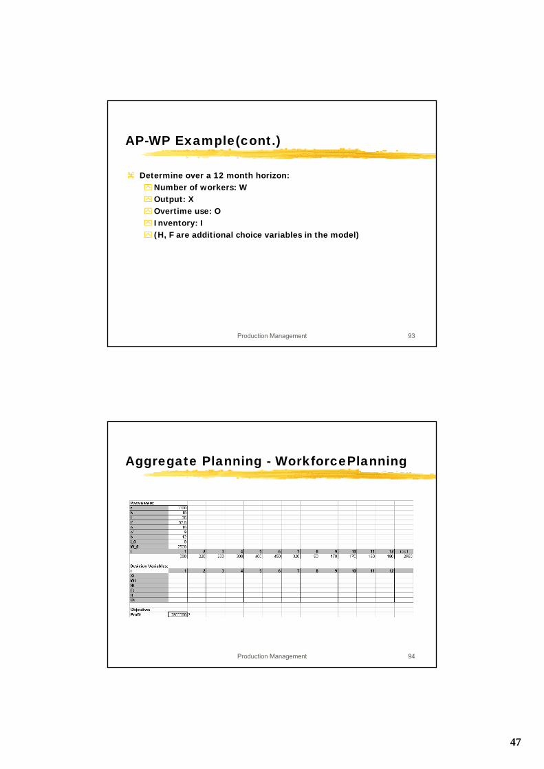
AP-WP Example
Revenue: 1000$worker capacity: 168h/monthinitially 15 workersno initial inventoryholding costs: 10$/unit/monthregular labor costs: 35$/hourovertime: 150% of regularhiring costs: 2500$ (2500/168 ~ 15$ per man-hour)lay-off costs: 1500$ (1500/168 ~ 9$ per man-hour)
no backorderingdemands over 12 months:
200, 220, 230, 300, 400, 450, 320, 180, 170,170, 160, 180demands must be met! (S=D)
47
Production Management 93
AP-WP Example(cont.)
Determine over a 12 month horizon:Number of workers: WOutput: XOvertime use: OInventory: I(H, F are additional choice variables in the model)
Production Management 94
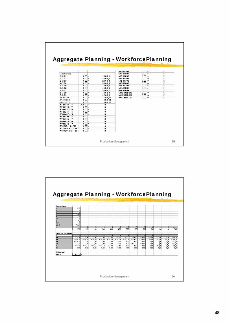
Aggregate Planning - WorkforcePlanning
48
Production Management 95
Aggregate Planning - WorkforcePlanning
Production Management 96
Aggregate Planning - WorkforcePlanning
49
Production Management 97
Aggregate Planning-Summary
The following scenarios have been discussed:
single product, single resource, single processfind: workforce, output, inventory (w. or w/o backorders)
multiple products, single resource, single processfind: workforce, all outputs, all inventories (w. or w/o backorders)
multiple products, multiple resources, multiple processes(workforce given)find: all outputs, all inventories, use of processes
Production Management 98
Aggregate Planning-Summary
The following scenarios have been discussed:
multiple products, multiple workstations(workstation capcities given)find: all sales, all outputs, all inventories (w. or w/o backorders)
multiple products, multiple workstationsfind: all sales, all outputs, all inventories (w. or w/o backorders), OT
single product, multiple workstations, one resourcefind: workforce, all sales, all outputs, all inventories (w. or w/o backorders),
OT
50
Production Management 99
Aggregate Planning
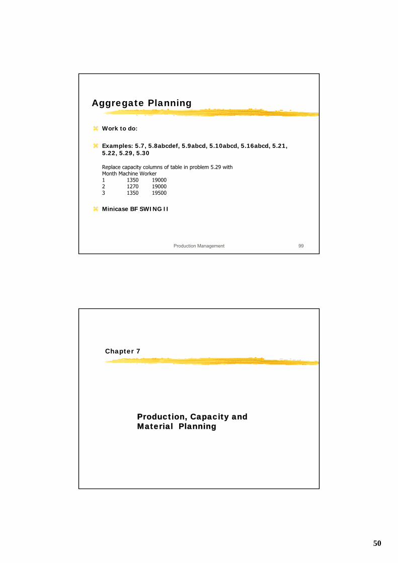
Work to do:
Examples: 5.7, 5.8abcdef, 5.9abcd, 5.10abcd, 5.16abcd, 5.21, 5.22, 5.29, 5.30
Replace capacity columns of table in problem 5.29 withMonth Machine Worker1 1350 190002 1270 190003 1350 19500
Minicase BF SWING II
Chapter 7
Production, Capacity and Material Planning
51
Production Management 101
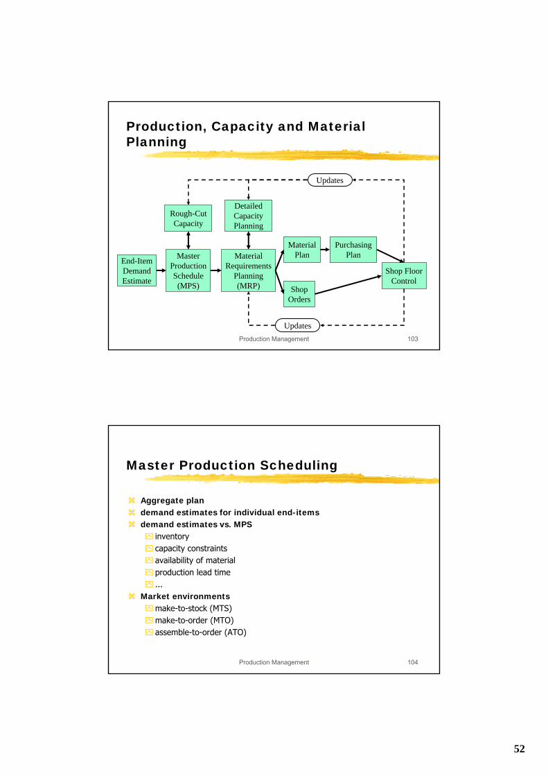
Production, Capacity and Material Planning
Production planquantities of final product, subassemblies, parts needed at distinct points in time
To generate the Production plan we need:end-product demand forecasts
Master production schedule
Master production schedule (MPS)delivery plan for the manufacturing organization
exact amounts and delivery timings for each end product
accounts for manufacturing constraints and final goods inventory
Production Management 102
Production, Capacity and Material Planning
Based on the MPS:
rough-cut capacity planning
Material requirements planningdetermines material requirements and timings for each phase of productiondetailed capacity planning
52
Production Management 103
End-Item Demand Estimate
Master Production Schedule (MPS)
Rough-Cut Capacity
Material Requirements
Planning (MRP)
Detailed Capacity Planning
Material Plan
Shop Orders
Purchasing Plan
Shop Floor Control
Updates
Updates
Production, Capacity and Material Planning
Production Management 104
Master Production Scheduling
Aggregate plandemand estimates for individual end-itemsdemand estimates vs. MPS
inventorycapacity constraintsavailability of materialproduction lead time...
Market environmentsmake-to-stock (MTS)make-to-order (MTO)assemble-to-order (ATO)
53
Production Management 105
Master Production Scheduling
MTSproduces in batchesminimizes customer delivery times at the expense of holding finished-goods inventoryMPS is performed at the end-item levelproduction starts before demand is known preciselysmall number of end-items, large number of raw-material items
MTOno finished-goods inventory customer orders are backloggedMPS is order driven, consisits of firm delivery dates
Production Management 106
Master Production Scheduling
ATOlarge number of end-items are assembled from a relatively small set of standard subassemblies, or modulesautomobile industryMPS governs production of modules (forecast driven)Final Assembly Schedule (FAS) at the end-item level (order driven)2 lead times, for consumer orders only FAS lead time relevant
54
Production Management 107
Master Production Scheduling
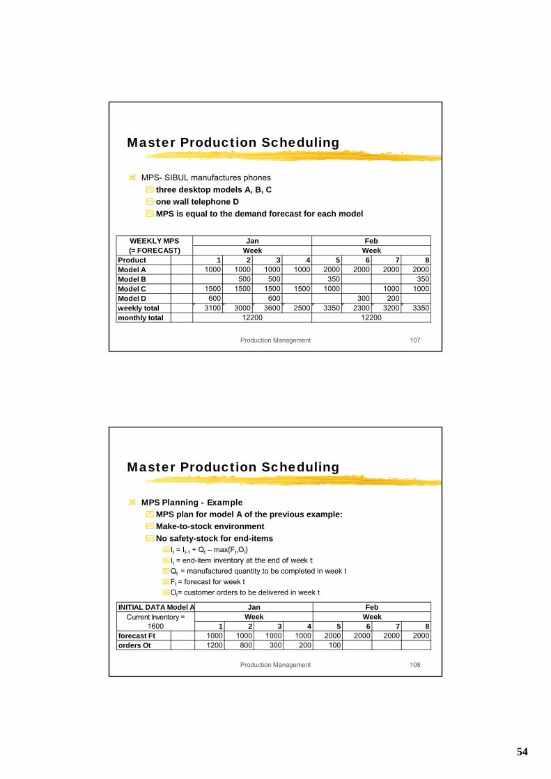
MPS- SIBUL manufactures phonesthree desktop models A, B, Cone wall telephone DMPS is equal to the demand forecast for each model
Product 1 2 3 4 5 6 7 8Model A 1000 1000 1000 1000 2000 2000 2000 2000Model B 500 500 350 350Model C 1500 1500 1500 1500 1000 1000 1000Model D 600 600 300 200weekly total 3100 3000 3600 2500 3350 2300 3200 3350monthly total
WEEKLY MPS (= FORECAST)
12200 12200
Jan FebWeek Week
Production Management 108
Master Production Scheduling
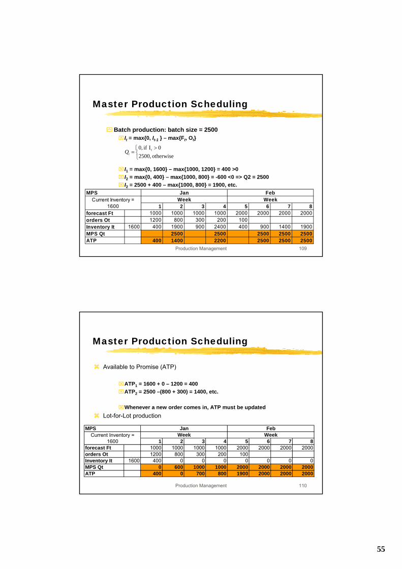
MPS Planning - ExampleMPS plan for model A of the previous example:Make-to-stock environmentNo safety-stock for end-items⌧It = It-1 + Qt – max{Ft,Ot}⌧It = end-item inventory at the end of week t ⌧Qt = manufactured quantity to be completed in week t⌧Ft = forecast for week t⌧Ot= customer orders to be delivered in week t
1 2 3 4 5 6 7 8forecast Ft 1000 1000 1000 1000 2000 2000 2000 2000orders Ot 1200 800 300 200 100
INITIAL DATA Model AWeek WeekJan Feb
Current Inventory = 1600
55
Production Management 109
Master Production Scheduling
Batch production: batch size = 2500⌧It = max{0, It-1 } – max{Ft, Ot}
⌧I1 = max{0, 1600} – max{1000, 1200} = 400 >0⌧I2 = max{0, 400} – max{1000, 800} = -600 <0 => Q2 = 2500⌧I2 = 2500 + 400 – max{1000, 800} = 1900, etc.
⎩⎨⎧ >
=otherwise ,2500
0I if ,0 ttQ
1 2 3 4 5 6 7 8forecast Ft 1000 1000 1000 1000 2000 2000 2000 2000orders Ot 1200 800 300 200 100Inventory It 1600 400 1900 900 2400 400 900 1400 1900MPS Qt 2500 2500 2500 2500 2500ATP 400 1400 2200 2500 2500 2500
MPS Jan FebCurrent Inventory =
1600Week Week
Production Management 110
Master Production Scheduling
Available to Promise (ATP)
⌧ATP1 = 1600 + 0 – 1200 = 400⌧ATP2 = 2500 –(800 + 300) = 1400, etc.
⌧Whenever a new order comes in, ATP must be updatedLot-for-Lot production
1 2 3 4 5 6 7 8forecast Ft 1000 1000 1000 1000 2000 2000 2000 2000orders Ot 1200 800 300 200 100Inventory It 1600 400 0 0 0 0 0 0 0MPS Qt 0 600 1000 1000 2000 2000 2000 2000ATP 400 0 700 800 1900 2000 2000 2000
MPS Jan FebCurrent Inventory =
1600Week Week
56
Production Management 111
Master Production Scheduling
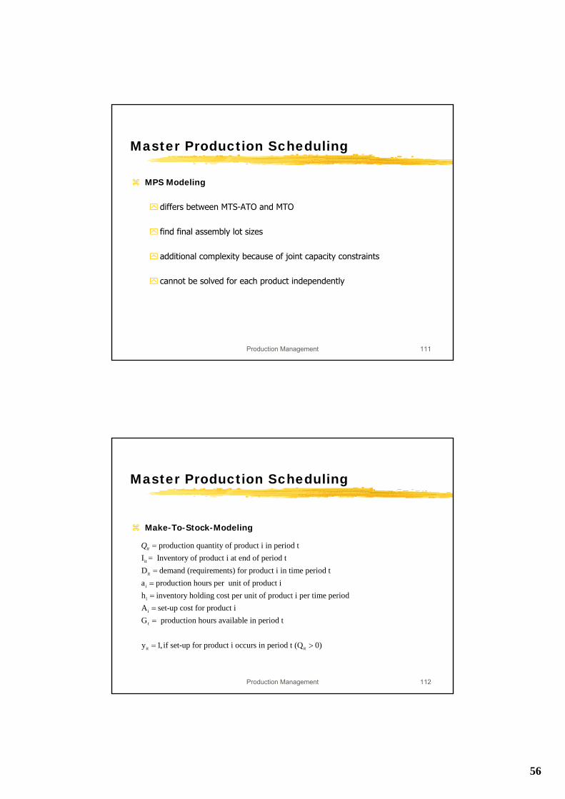
MPS Modeling
differs between MTS-ATO and MTO
find final assembly lot sizes
additional complexity because of joint capacity constraints
cannot be solved for each product independently
Production Management 112
Make-To-Stock-Modeling
Master Production Scheduling
it
it
i
i
production quantity of product i in period tI = Inventory of product i at end of period tD demand (requirements) for product i in time period ta production hours per unit of product ih inve
itQ =
===
i
t
it it
ntory holding cost per unit of product i per time periodA set-up cost for product iG production hours available in period t
y 1, if set-up for product i occurs in period t (Q 0)
==
= >
57
Production Management 113
Make-To-Stock-Modeling
Master Production Scheduling
( )1 1
, -1
i1
it1
it
min
for all (i,t)
a for all t
Q 0 for all (i,t)
Q 0; 0; {0,1}
n T
i it i iti t
i t it it it
n
it ti
T
it ikk
it it
A y h I
I Q I D
Q G
y D
I y
= =
=
=
+
+ − =
≤
− ≤
≥ ≥ ∈
∑∑
∑
∑
Production Management 114
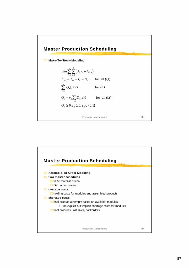
Assemble-To-Order Modelingtwo master schedules
MPS: forecast-drivenFAS: order driven
overage costsholding costs for modules and assembled products
shortage costsfinal product assemply based on available modules
no explicit but implicit shortage costs for modulesfinal products: lost sales, backorders
Master Production Scheduling
58
Production Management 115
Master Production Scheduling
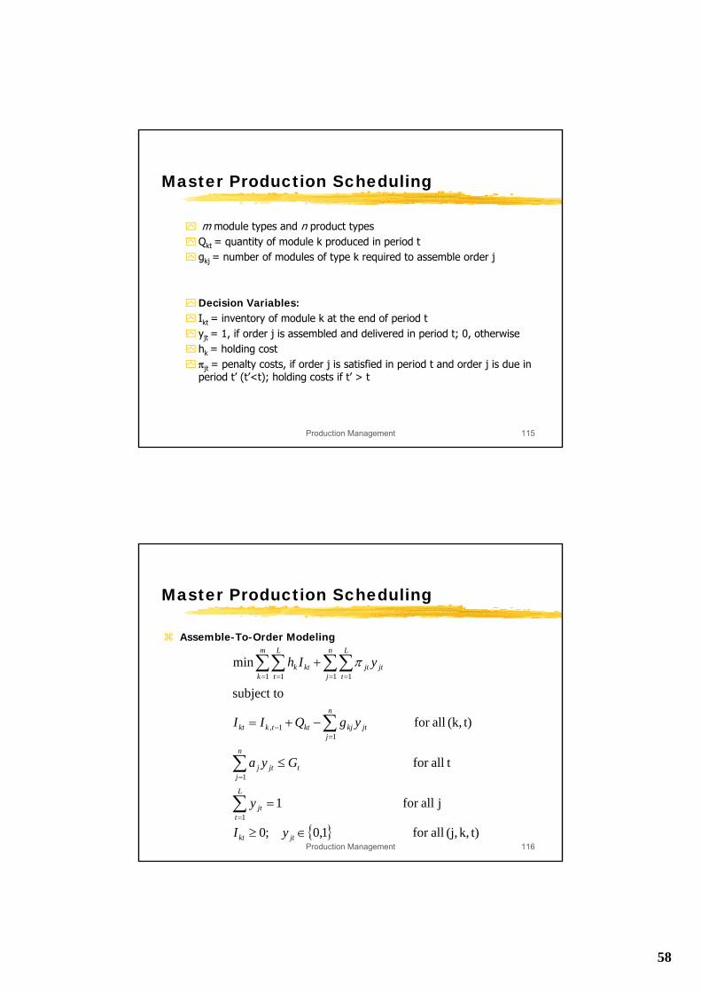
m module types and n product typesQkt = quantity of module k produced in period tgkj = number of modules of type k required to assemble order j
Decision Variables:Ikt = inventory of module k at the end of period t yjt = 1, if order j is assembled and delivered in period t; 0, otherwisehk = holding cost πjt = penalty costs, if order j is satisfied in period t and order j is due in period t’ (t’<t); holding costs if t’ > t
Production Management 116
Assemble-To-Order Modeling
Master Production Scheduling
{ } t)k,(j, allfor 1,0;0
j allfor 1
tallfor
t)(k, allfor
subject to
min
1
1
11,
1 1 1 1
∈≥
=
≤
−+=
+
∑
∑
∑
∑∑ ∑∑
=
=
=−
= = = =
jtkt
L
tjt
n
jtjtj
n
jjtkjkttkkt
m
k
L
t
n
j
L
tjtjtktk
yI
y
Gya
ygQII
yIh π
59
Production Management 117
Master Production Scheduling
Capacity PlanningBottleneck in production facilitiesRough-Cut Capacity Planning (RCCP) at MPS levelfeasibilitydetailed capacity planning (CRP) at MRP levelboth RCCP and CRP are only providing information
Production Management 118
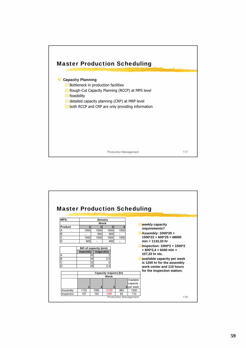
Master Production SchedulingMPS:
Product 1 2 3 4A 1000 1000 1000 1000B - 500 500 -C 1500 1500 1500 1500D 600 - 600 -
JanuaryWeek
Assembly InspectionA 20 2B 24 2.5C 22 2D 25 2.4
Bill of capacity (min)
⌧weekly capacity requirements?
⌧Assembly: 1000*20 + 1500*22 + 600*25 = 68000 min = 1133,33 hr
⌧Inspection: 1000*2 + 1500*2 + 600*2,4 = 6440 min = 107,33 hr etc.
⌧available capacity per week is 1200 hr for the assembly work center and 110 hours for the inspection station;
1 2 3 4
Available capacity per week
Assembly 1133 1083 1333!! 883 1200Inspection 107 104 128!! 83 110
Capacity requires (hr)Week
60
Production Management 119
Master Production Scheduling
Infinite capacity planning (information providing)finding a feasible cost optimal solution is a NP-hard problem
if no detailed bill of capacity is available: capacity planning using overall factors (globale Belastungsfaktoren)
required input:MPSstandard hours of machines or direct labor requiredhistorical data on individual shop workloads (%)
Example from Günther/TempelmeierC133.3: overall factors
Production Management 120
Master Production Scheduling
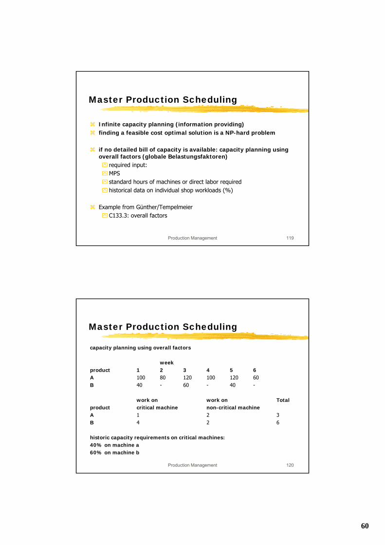
capacity planning using overall factors
weekproduct 1 2 3 4 5 6A 100 80 120 100 120 60B 40 - 60 - 40 -
work on work on Totalproduct critical machine non-critical machineA 1 2 3B 4 2 6
historic capacity requirements on critical machines:40% on machine a60% on machine b

61
Production Management 121
Master Production Scheduling
in total 500 working units are available per week, 80 on machine a and 120 on machine b;
Solution:overall factor = time per unit x historic capacity needs
product A:machine a: 1 x 0,4 = 0,4machine b: 1 x 0,6 = 0,6
product B:machine a: 4 x 0,4 = 1,6machine b: 4 x 0,6 = 2,4
Production Management 122
Master Production Schedulingcapacity requirements: product Amachine week
1 2 3 4 5 6a 40 32 48 40 48 24b 60 48 72 60 72 36other 200 160 240 200 240 120
capacity requirements: product Bmachine week
1 2 3 4 5 6a 64 - 96 - 64 -b 96 - 144 - 96 -other 80 - 120 - 80 -
62
Production Management 123
Master Production Scheduling
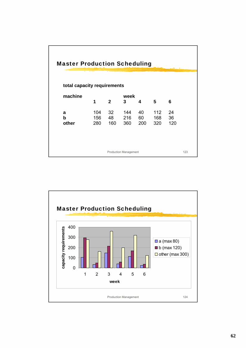
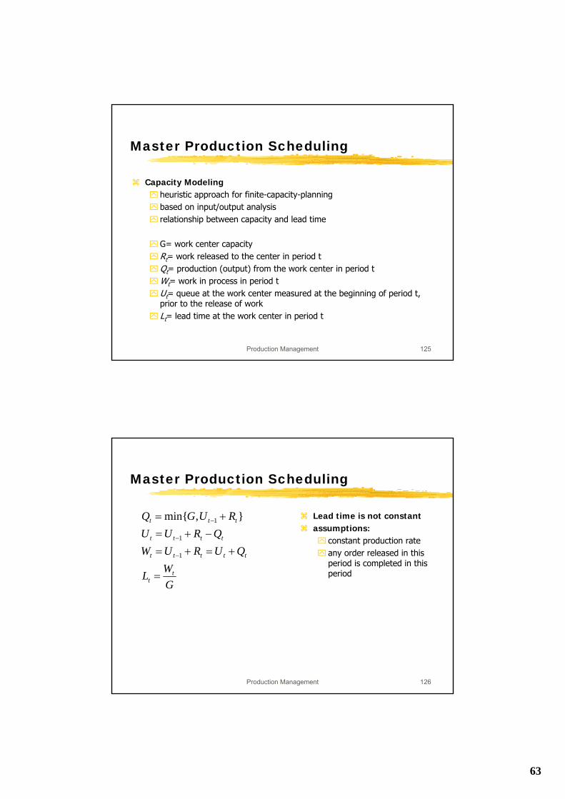
total capacity requirements machine week 1 2 3 4 5 6 a 104 32 144 40 112 24 b 156 48 216 60 168 36 other 280 160 360 200 320 120
Production Management 124
Master Production Scheduling
0
100
200
300
400
1 2 3 4 5 6week
capa
city
requ
irem
ents
a (max 80)b (max 120)other (max 300)
63
Production Management 125
Master Production Scheduling
Capacity Modelingheuristic approach for finite-capacity-planning based on input/output analysis relationship between capacity and lead time
G= work center capacityRt= work released to the center in period tQt= production (output) from the work center in period tWt= work in process in period tUt= queue at the work center measured at the beginning of period t, prior to the release of workLt= lead time at the work center in period t
Production Management 126
Master Production Scheduling
Lead time is not constantassumptions:
constant production rateany order released in this period is completed in this period
GWL
QURUWQRUU
RUGQ
tt
ttttt
tttt
ttt
=
+=+=−+=
+=
−
−
−
1
1
1 },min{
64
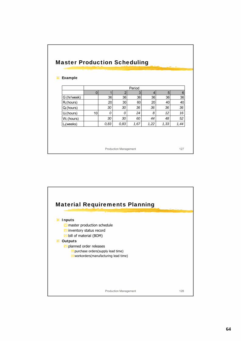
Production Management 127
Master Production Scheduling
Example
0 1 2 3 4 5 6G (hr/week) 36 36 36 36 36 36Rt (hours) 20 30 60 20 40 40Qt (hours) 30 30 36 36 36 36Ut (hours) 10 0 0 24 8 12 16Wt (hours) 30 30 60 44 48 52Lt(weeks) 0,83 0,83 1,67 1,22 1,33 1,44
Period
Production Management 128
Material Requirements Planning
Inputsmaster production scheduleinventory status recordbill of material (BOM)
Outputsplanned order releases⌧purchase orders(supply lead time)⌧workorders(manufacturing lead time)
65
Production Management 129
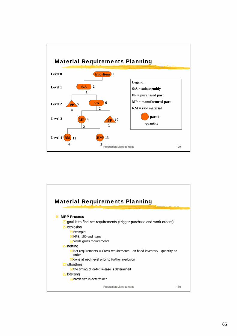
Material Requirements Planning
End-Item 1
S/A 21
PP 54
S/A 62
PP 101
MP 9
2
RM 13
2
RM 12
4
Level 0
Level 1
Level 2
Level 3
Level 4
Legend:
S/A = subassembly
PP = purchased part
MP = manufactured part
RM = raw material
part #
quantity
Production Management 130
Material Requirements Planning
MRP Processgoal is to find net requirements (trigger purchase and work orders)explosion⌧Example:⌧MPS, 100 end items⌧yields gross requirements
netting⌧Net requirements = Gross requirements - on hand inventory - quantity on
order ⌧done at each level prior to further explosion
offsetting⌧the timing of order release is determined
lotsizing⌧batch size is determined
66
Production Management 131
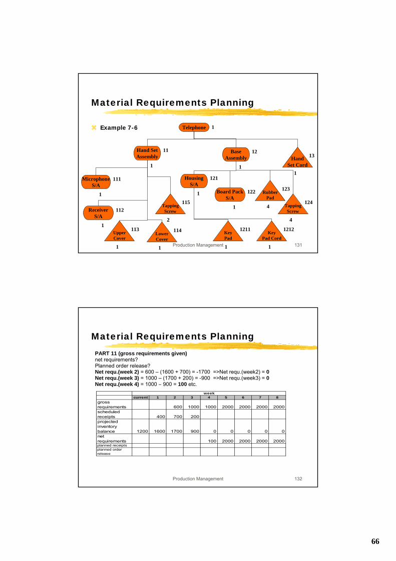
Material Requirements Planning
Example 7-6 Telephone 1
Hand SetAssembly
11
1
BaseAssembly
12
1Hand
Set Cord
13
1Housing
S/A121
1 Board PackS/A
122
1
RubberPad
123
4 TappingScrew
124
4
KeyPad
1211
1
KeyPad Cord
1212
1
MicrophoneS/A
111
1
ReceiverS/A
112
1UpperCover
113
1
LowerCover
114
1
TappingScrew
115
2
Production Management 132
Material Requirements PlanningPART 11 (gross requirements given)net requirements? Planned order release? Net requ.(week 2) = 600 – (1600 + 700) = -1700 =>Net requ.(week2) = 0 Net requ.(week 3) = 1000 – (1700 + 200) = -900 =>Net requ.(week3) = 0 Net requ.(week 4) = 1000 – 900 = 100 etc.
current 1 2 3 4 5 6 7 8gross requirements 600 1000 1000 2000 2000 2000 2000scheduled receipts 400 700 200projected inventory balance 1200 1600 1700 900 0 0 0 0 0net requirements 100 2000 2000 2000 2000planned receiptsplanned order release
week
67
Production Management 133
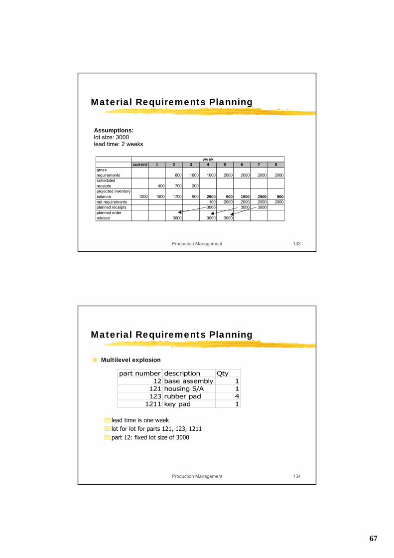
Material Requirements Planning
Assumptions:lot size: 3000lead time: 2 weeks
current 1 2 3 4 5 6 7 8gross requirements 600 1000 1000 2000 2000 2000 2000scheduled receipts 400 700 200projected inventory balance 1200 1600 1700 900 2900 900 1900 2900 900net requirements 100 2000 2000 2000 2000planned receipts 3000 3000 3000planned order release 3000 3000 3000
week
Production Management 134
Material Requirements Planning
Multilevel explosion
lead time is one weeklot for lot for parts 121, 123, 1211part 12: fixed lot size of 3000
part number description Qty12 base assembly 1
121 housing S/A 1123 rubber pad 4
1211 key pad 1
68
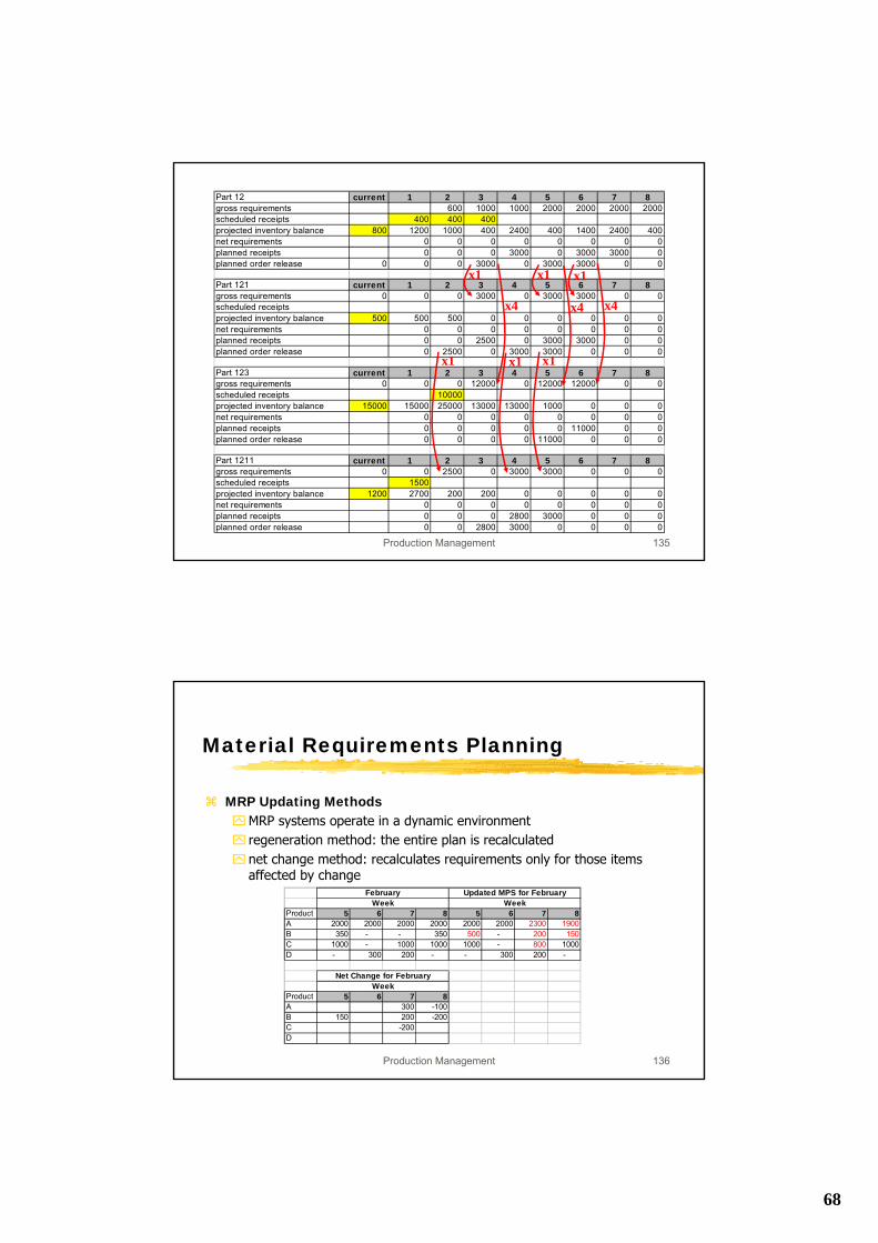
Production Management 135
Part 12 current 1 2 3 4 5 6 7 8gross requirements 600 1000 1000 2000 2000 2000 2000scheduled receipts 400 400 400projected inventory balance 800 1200 1000 400 2400 400 1400 2400 400net requirements 0 0 0 0 0 0 0 0planned receipts 0 0 0 3000 0 3000 3000 0planned order release 0 0 0 3000 0 3000 3000 0 0
Part 121 current 1 2 3 4 5 6 7 8gross requirements 0 0 0 3000 0 3000 3000 0 0scheduled receiptsprojected inventory balance 500 500 500 0 0 0 0 0 0net requirements 0 0 0 0 0 0 0 0planned receipts 0 0 2500 0 3000 3000 0 0planned order release 0 2500 0 3000 3000 0 0 0
Part 123 current 1 2 3 4 5 6 7 8gross requirements 0 0 0 12000 0 12000 12000 0 0scheduled receipts 10000projected inventory balance 15000 15000 25000 13000 13000 1000 0 0 0net requirements 0 0 0 0 0 0 0 0planned receipts 0 0 0 0 0 11000 0 0planned order release 0 0 0 0 11000 0 0 0
Part 1211 current 1 2 3 4 5 6 7 8gross requirements 0 0 2500 0 3000 3000 0 0 0scheduled receipts 1500projected inventory balance 1200 2700 200 200 0 0 0 0 0net requirements 0 0 0 0 0 0 0 0planned receipts 0 0 0 2800 3000 0 0 0planned order release 0 0 2800 3000 0 0 0 0
x1 x1 x1
x4 x4 x4
x1 x1x1
Production Management 136
Material Requirements Planning
MRP Updating MethodsMRP systems operate in a dynamic environmentregeneration method: the entire plan is recalculatednet change method: recalculates requirements only for those items affected by change
Product 5 6 7 8 5 6 7 8A 2000 2000 2000 2000 2000 2000 2300 1900B 350 - - 350 500 - 200 150C 1000 - 1000 1000 1000 - 800 1000D - 300 200 - - 300 200 -
Product 5 6 7 8A 300 -100B 150 200 -200C -200D
Net Change for FebruaryWeek
Updated MPS for FebruaryWeek
FebruaryWeek
69
Production Management 137
Material Requirements Planning
Additional Netting proceduresimplosion: ⌧opposite of explosion⌧finds common item
combining requirements:⌧process of obtaining the gross requirements of a common item
pegging: ⌧identify the item’s end product⌧useful when item shortages occur
Production Management 138
Material Requirements Planning
Lot Sizing in MRPminimize set-up and holding costs
can be formulated as MIP
a variety of heuristic approaches are available
simplest approach: use independent demand procedures (e.g. EOQ) at every level
70
Production Management 139
Material Requirements Planning
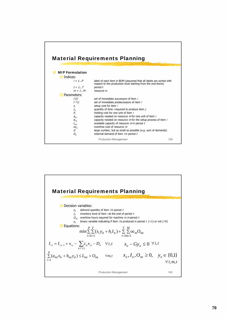
MIP FormulationIndices:
i = 1...P label of each item in BOM (assumed that all labels are sorted withrespect to the production level starting from the end-items)
t = 1...T period tm = 1...M resource m
Parameters:Γ(i) set of immediate successors of item iΓ-1(i) set of immediate predeccessors of item isi setup cost for item icij quantity of itme i required to produce item jhi holding cost for one unit of item iami capacity needed on resource m for one unit of item ibmi capacity needed on resource m for the setup process of item iLmt available capacity of resource m in period tocm overtime cost of resource mG large number, but as small as possible (e.g. sum of demands)Dit external demand of item i in period t
Production Management 140
Material Requirements Planning
Decision variables:xit deliverd quantity of item i in period tIit inventory level of item i at the end of period tOmt overtime hours required for machine m in period tyit binary variable indicating if item i is produced in period t (=1) or not (=0)
Equations:
mtT
t
M
mm
P
i
T
titiiti OocIhys ∑ ∑+∑∑ +
= == = 1 11 1)(min
itij
jtijtititi DxcxII −−+= ∑Γ∈
−)(
,1,,
)(1
mtmtP
iitmiitmi OLybxa +≤∑ +
=
0≤− itit Gyxti,∀
tm,∀
ti,∀
}1,0{,0,, ∈≥ itmtitit yOIxtmi ,,∀
71
Production Management 141
Material Requirements Planning
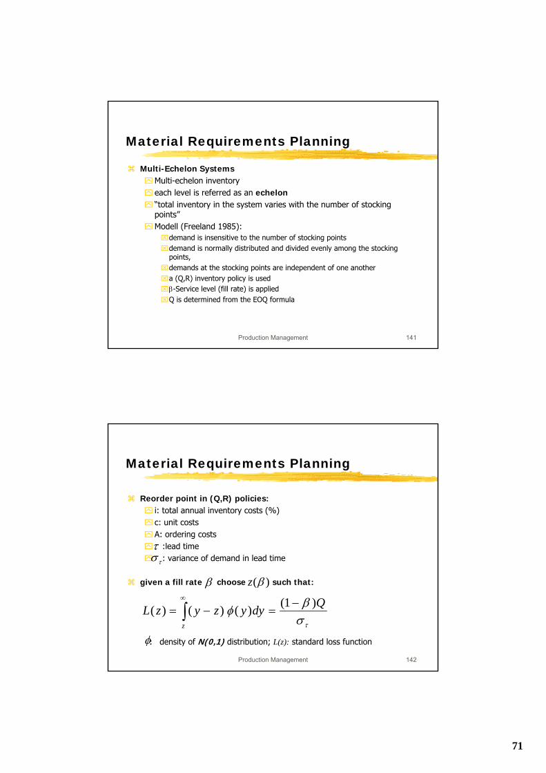
Multi-Echelon SystemsMulti-echelon inventoryeach level is referred as an echelon“total inventory in the system varies with the number of stockingpoints”Modell (Freeland 1985):⌧demand is insensitive to the number of stocking points⌧demand is normally distributed and divided evenly among the stocking
points, ⌧demands at the stocking points are independent of one another⌧a (Q,R) inventory policy is used⌧β-Service level (fill rate) is applied⌧Q is determined from the EOQ formula
Production Management 142
Material Requirements Planning
Reorder point in (Q,R) policies:i: total annual inventory costs (%)c: unit costsA: ordering costs
:lead time: variance of demand in lead time
given a fill rate choose such that:
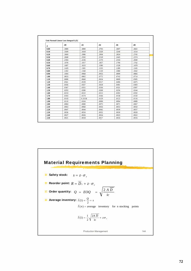
: density of N(0,1) distribution; L(z): standard loss function
ττσ
β )(βz
∫∞ −
=−=z
QdyyzyzLτσβφ )1()()()(
φ
72
Production Management 143
Unit Normal Linear Loss Integral L(Z)
.0016.0016.0017.0018.00212.50
.0022.0023.0024.0026.00272.40
.0028.0030.0032.0034.00362.30
.0037.0039.0042.0044.00472.20
.0050.0053.0056.0060.00632.10
.0067.0071.0075.0080.00842.00
.0089.0094.0099.0104.01101.90
.0116.0122.01290..0136.01431.80
.0150.0158.0166.0174.01831.70
.0192.0202.0212.0222.02331.60
.0244.0256.0268.0280.02931.50
.0307.0321.0336.0351.03671.40
.0383.0401.0418.0437.04561.30
.0475.0496.0517.0539.05611.20
.0585.0609.0634.0660.06861.10
.0714.0742.0772.0802.08331.00
.0866.0899.0933.0968.10040.90
.1042.1080.1120.1160.12020.80
.1245.1289.1335.1381.14290.70
.1478.1528.1580.1633.16870.60
.1742.1799.1857.1917.19780.50
.2040.2104.2170.2236.23040.40
.2374.2445.2518.2592.26680.30
.2745.2824.2904.2986.30690.20
.3154.3240.3329.3418.35090.10
.3602.3697.3793.3890.39890.00
.08.06.04.02.00Z
Production Management 144
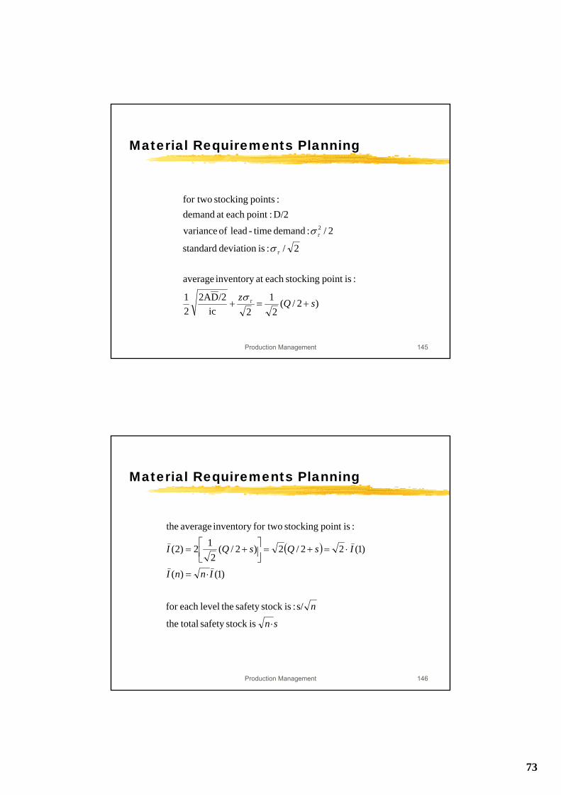
τσ⋅= zs
τσzI
nI
sQI
+=
=
+=
icD2A
21)1(
points stockingn for inventoryaverage )(2
)1(
Material Requirements Planning
Safety stock:
Reorder point:
Order quantity:
Average inventory:
ττ σ⋅+= zDR
icDAEOQQ 2
==
73
Production Management 145
Material Requirements Planning
)2/(2
12ic
/2D2A21
:ispoint stockingeach at inventory average
2/ :isdeviation standard
2/ :demand time-lead of varianceD/2 :pointeach at demand:points stocking for two
2
sQz+=+ τ
τ
τ
σ
σ
σ
Production Management 146
Material Requirements Planning
( )
sn
n
InnI
IsQsQI
⋅
⋅=
⋅=+=⎥⎦⎤
⎢⎣⎡ +=
isstock safety totalthe
s/ :isstock safety theleveleach for
)1()(
)1(22/2)2/(2
12)2(
:ispoint stocking for twoinventory average the
74
Production Management 147
Material Requirements Planning
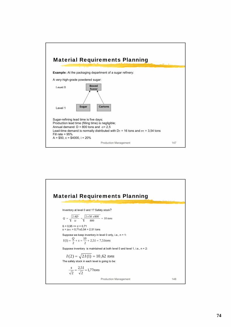
Example: At the packaging department of a sugar refinery:
A very-high-grade powdered sugar:
Sugar-refining lead time is five days;Production lead time (filling time) is negligible;Annual demand: D = 800 tons and σ= 2,5Lead-time demand is normally distributed with Dτ = 16 tons and στ = 3,54 tonsFill rate = 95%A = $50, c = $4000, i = 20%
BoxedSugar
Sugar Cartons
Level 0
Level 1
Production Management 148
Material Requirements Planning
Inventory at level 0 and 1? Safety stock?
ß = 0,95 => z = 0,71s = zστ = 0,71x3,54 = 2,51 tons
Suppose we keep inventory in level 0 only, i.e., n = 1:
Suppose inventory is maintained at both level 0 and level 1, i.e., n = 2:
The safety stock in each level is going to be:
tonsxxicADQ 10
8008005022
===
tonssQI 51,751,22
102
)1( =+=+=
tonsII 62,10)1(2)2( ==
tonss 77,1251,2
2==
75
Production Management 149
Material Requirements Planning
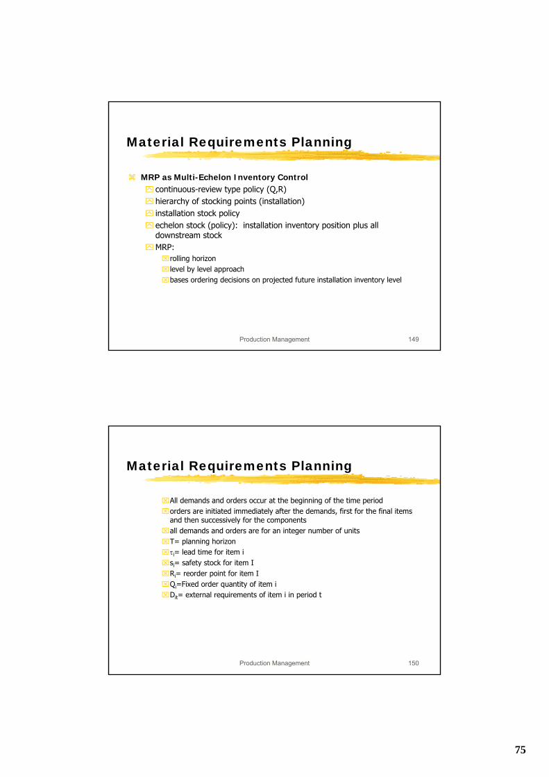
MRP as Multi-Echelon Inventory Controlcontinuous-review type policy (Q,R)hierarchy of stocking points (installation)installation stock policyechelon stock (policy): installation inventory position plus all downstream stockMRP:⌧rolling horizon ⌧level by level approach⌧bases ordering decisions on projected future installation inventory level
Production Management 150
Material Requirements Planning
⌧All demands and orders occur at the beginning of the time period⌧orders are initiated immediately after the demands, first for the final items
and then successively for the components⌧all demands and orders are for an integer number of units⌧T= planning horizon⌧τi= lead time for item i⌧si= safety stock for item I⌧Ri= reorder point for item I⌧Qi=Fixed order quantity of item i ⌧Dit= external requirements of item i in period t
76
Production Management 151
Material Requirements Planning
Installation stock policies (Q,Ri) for MRP:a production order is triggered if the installation stock minus safety stock is insufficient to cover the requirements over the next τi periodsan order may consist of more than one order quantity Q
if lead time τi = 0, the MRP is equal to an installation stock policy.safety stock = reorder point
Production Management 152
Material Requirements Planning
Echelon stock policies (Q,Re) for MRP:Consider a serial assembly systemInstallation 1 is the downstream installation (final product)the output of installation i is the input when producing one unit of item i-1 at the immediate downstream installationwi = installation inventory position at installation iIi = echelon inventory position at installation i (at the same moment)
Ii = wi+ wi-1+... w1
a multi-echelon (Q,R) policy is denoted by (Qi,Rie)
Rie gives the reorder point for echelon inventory at i
77
Production Management 153
Material Requirements Planning
R1e = s1+Dτ1
Rie = si+Dτi+Ri-1
e +Qi-1
Example:
Two-level system, 6 periods
D = 2 (Item 1), τ1 = 1, τ2 = 230,10,34,20,38,18 2121
02
01 ====== QQRRII ee
Production Management 154
Material Requirements Planning
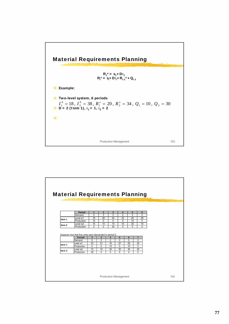
Period 1 2 3 4 5 6Demand 2 2 2 2 2 2Level w1 18 26 24 22 20 28Production 10 0 0 0 10 0Level w2 10 10 10 10 30 10Production 0 0 30 0 0 0
Item 1
Item 2
Suppose now that five units were demanded in period 2:Period 2 3 4 5 6 7
Demand 5 2 2 2 2 2Level w1 23 21 19 27 25 23Production 0 0 10 0 10 0Level w2 10 10 30 30 30 30Production 30 0 0 0 0 0
Item 1
Item 2
78
Production Management 155
Material Requirements Planning
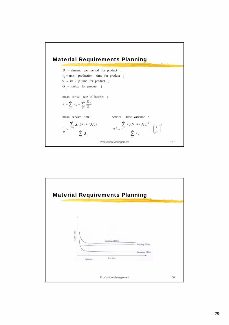
Lot Size and Lead Timelead time is affected by capacity constraintslot size affects lead time
batching effectan increase in lot size should increase lead time
saturation effectwhen lot size decreases, and set-up is not reduced, lead time will increase
expected lead time can be calculated using models from queueingtheory (M/G/1)
Production Management 156
Material Requirements Planning
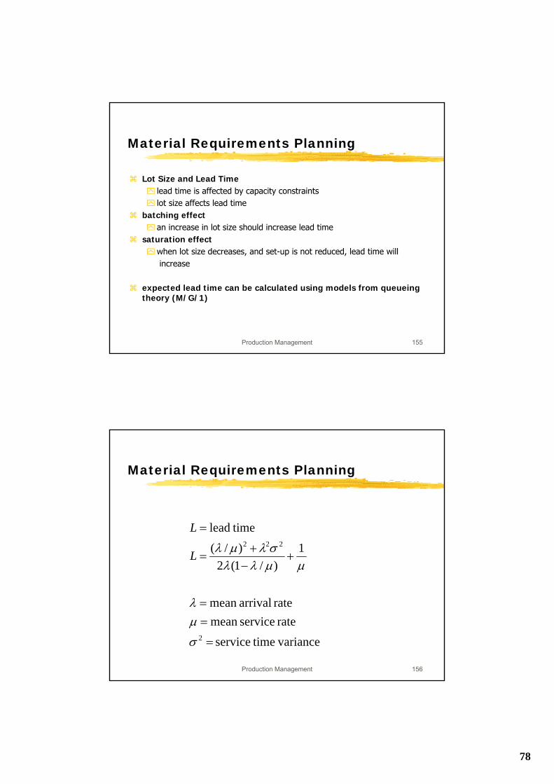
variance timeservice rate servicemean
rate arrivalmean
1)/1(2
)/( timelead
2
222
=
==
+−+
=
=
σ
μλ
μμλλσλμλL
L
79
Production Management 157
Material Requirements Planning
2
1
1
2
2n
1jj
1
1 1
j
j
j
1)()(
1
: variancetime-service: timeservicemean
:batches of rate arrivalmean
jproduct for lotsizeQ
jproduct for timeup-setS
jproduct for timeproduction-unitt
jproduct for periodper demand
⎟⎟⎠
⎞⎜⎜⎝
⎛−
+=
+=
==
=
=
=
=
∑
∑
∑
∑
∑ ∑
=
=
=
=
= =
μλ
λσ
μ
λλ
λ
λn
jj
n
jjjjjjjj
n
jj
n
j
n
j j
jj
j
QtSQtS
QD
D
Production Management 158
Material Requirements Planning
80
Production Management 159
Material Planning
Work to do: 7.7ab, 7.8, 7.10, 7.11, 7.14 (additional information: available hours: 225 (Paint), 130 (Mast), 100 (Rope)), 7.15, 7.16, 7.17, 7.31-7.34
Chapter 8
Operations Scheduling
81
Production Management 161
Operations Scheduling
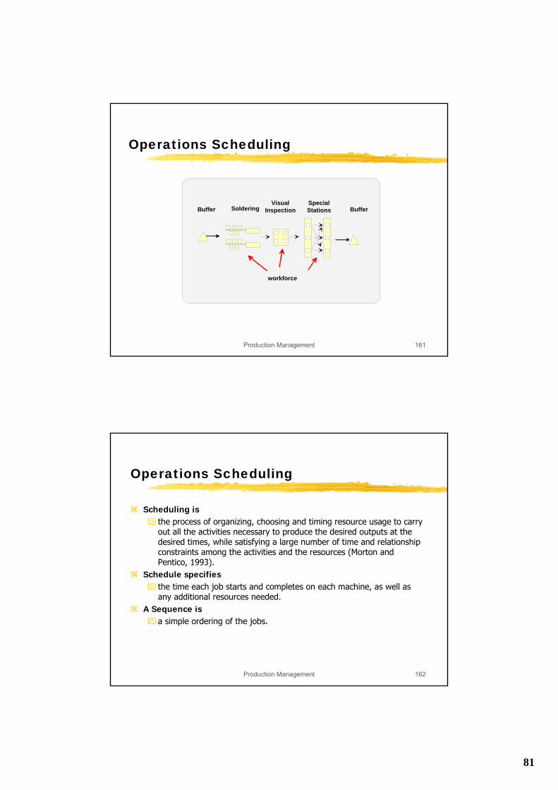
SolderingBuffer Buffer
workforce
VisualInspection
SpecialStations
Production Management 162
Operations Scheduling
Scheduling is the process of organizing, choosing and timing resource usage to carry out all the activities necessary to produce the desired outputs at the desired times, while satisfying a large number of time and relationship constraints among the activities and the resources (Morton and Pentico, 1993).
Schedule specifiesthe time each job starts and completes on each machine, as well as any additional resources needed.
A Sequence isa simple ordering of the jobs.
82
Production Management 163
Determining a best sequence32 jobs on a single machine32! Possible sequences approx. 2.6x1035
⌧suppose a computer could examine one billion sequences per second⌧it would take 8.4x10¹⁵ centuries
real life problems are much more complicatedScheduling theory helps to ⌧classify the problems⌧identify appropriate measures⌧develop solution procedures
Operations Scheduling
Production Management 164
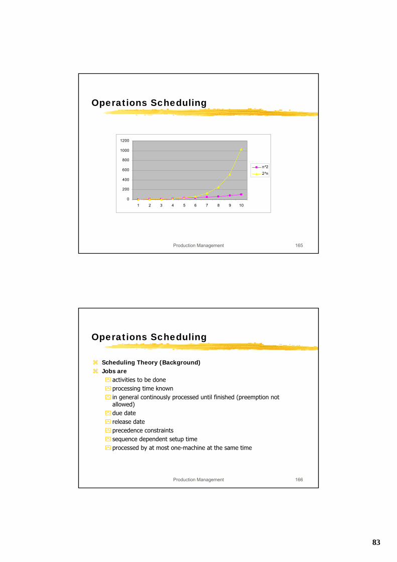
Algorithmic complexityan efficient algorithm is one whose effort of any problem instance is bounded by a polynomial in the problem size, e.g. # of jobsminimal spanning tree can be solved in at most n2 iterationsn: number of edgesO(n2)
if effort is exponential O(2n) the algorithm is not efficientbranch and bound algorithm for 0/1 variables
NP-hard problems: no exact algorithm in polynomial time is known. e.g. Traveling salesman problemHeuristics are usually polynomial algorithms tailored to the specific problem structure
Operations Scheduling
83
Production Management 165
Operations Scheduling
0
200
400
600
800
1000
1200
1 2 3 4 5 6 7 8 9 10
n^2
2^n
Production Management 166
Scheduling Theory (Background)Jobs are
activities to be doneprocessing time knownin general continously processed until finished (preemption not allowed)due date release dateprecedence constraintssequence dependent setup timeprocessed by at most one-machine at the same time
Operations Scheduling
84
Production Management 167
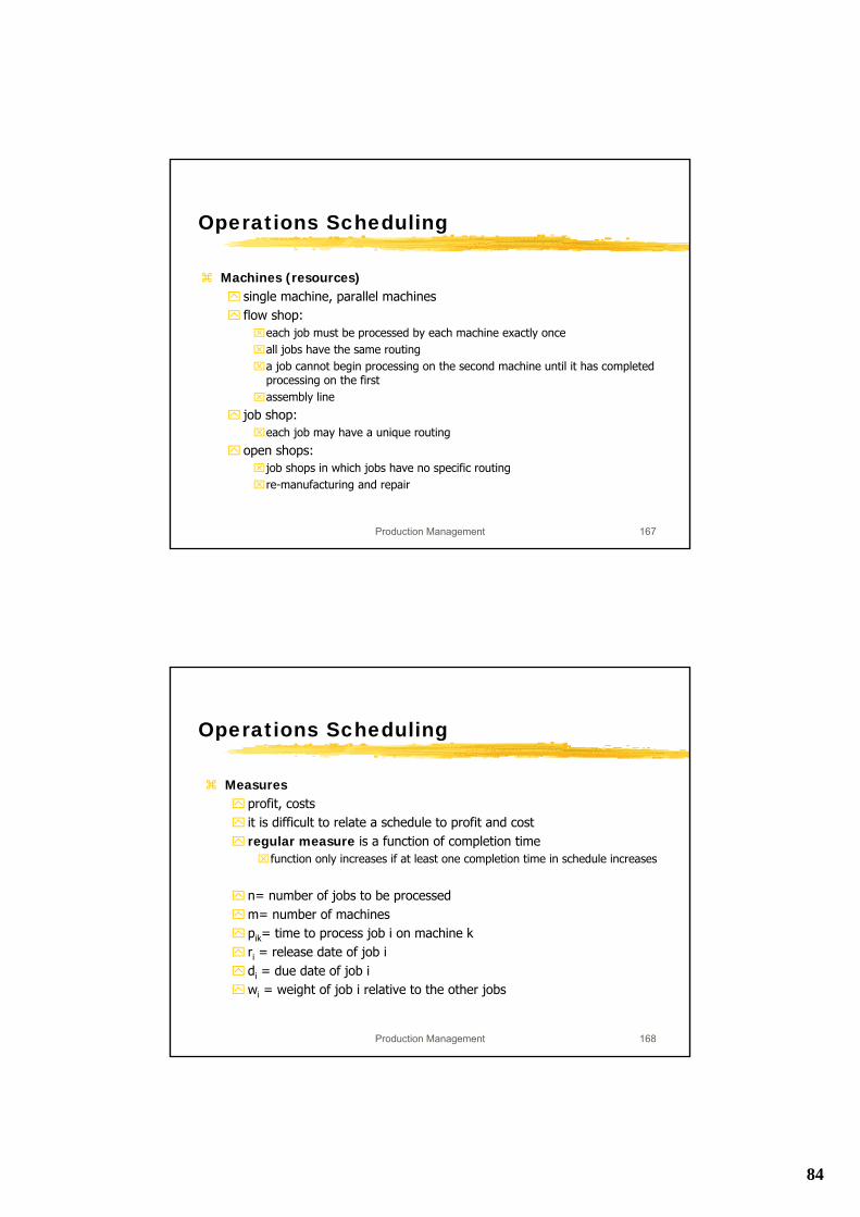
Machines (resources)single machine, parallel machinesflow shop: ⌧each job must be processed by each machine exactly once⌧all jobs have the same routing⌧a job cannot begin processing on the second machine until it has completed
processing on the first⌧assembly line
job shop:⌧each job may have a unique routing
open shops:⌧job shops in which jobs have no specific routing⌧re-manufacturing and repair
Operations Scheduling
Production Management 168
Measuresprofit, costsit is difficult to relate a schedule to profit and costregular measure is a function of completion time⌧function only increases if at least one completion time in schedule increases
n= number of jobs to be processedm= number of machinespik= time to process job i on machine kri = release date of job idi = due date of job iwi = weight of job i relative to the other jobs
Operations Scheduling
85
Production Management 169
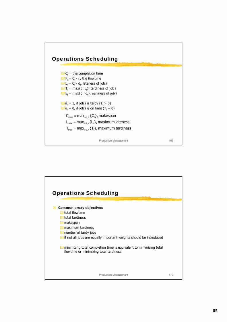
Ci = the completion timeFi = Ci - ri, the flowtimeLi = Ci - di, lateness of job iTi = max{0, Li}, tardiness of job iEi = max{0, -Li}, earliness of job i
δi = 1, if job i is tardy (Ti > 0)δi = 0, if job i is on time (Ti = 0)
Operations Scheduling
tardiness maximum },{Tmax T
lateness maximum },{Lmax L
makespan},{Cmax C
in1,imax
in1,imax
in1,imax
=
=
=
=
=
=
Production Management 170
Operations Scheduling
Common proxy objectivestotal flowtimetotal tardinessmakespanmaximum tardinessnumber of tardy jobsif not all jobs are equally important weights should be introduced
minimizing total completion time is equivalent to minimizing total flowtime or minimizing total tardiness
86
Production Management 171
Operations Scheduling
Algorithms:exact algorithms often based on (worst case scenario) enumeration (e.g. Branch and Bound, Dynamic Programming)
heuristic algorithm judged by quality (difference to the optimalsolution) and efficacy (computational effort)worst-case bounds are desirable to motivate use of a certain heuristic
Production Management 172
Operations Scheduling
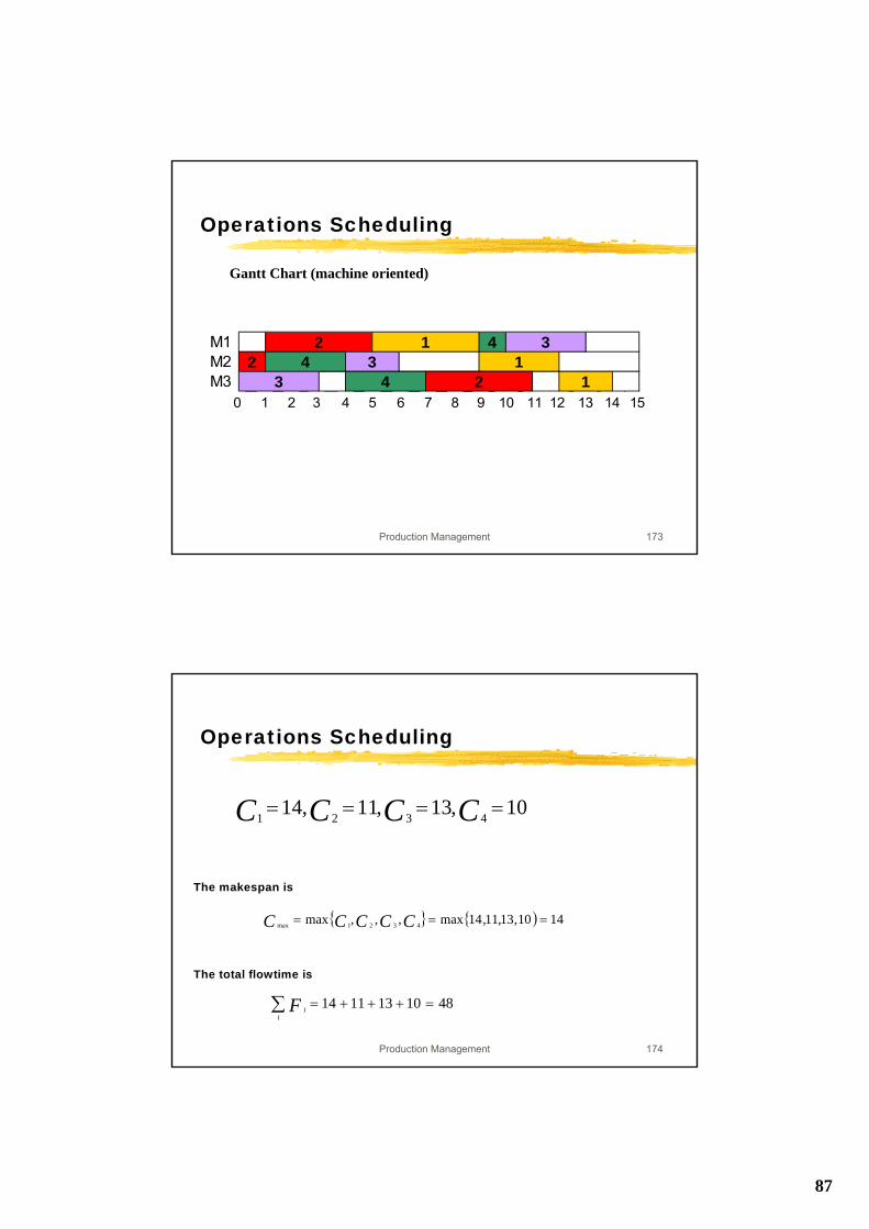
Assume the following sequences:2-1-4-3 on M12-4-3-1 on M23-4-2-1 on M3
Consider the following four-job, three-machine job-shop scheduling problem:
Processing time/machine number
Job Op.1 Op.2 Op.3 Release Date Due date
1 4/1 3/2 2/3 0 162 1/2 4/1 4/3 0 143 3/3 2/2 3/1 0 104 3/2 3/3 1/1 0 8
87
Production Management 173
Operations Scheduling
Gantt Chart (machine oriented)
M1 4M2 2M3 2
11
133
34
4
2
0 1 2 3 4 5 6 7 8 9 10 11 12 13 14 15
Production Management 174
Operations Scheduling
The makespan is
The total flowtime is
{ } ){ 1410,13,11,14max,,,max 4321max === CCCCC
4810131114 =+++=∑i
iF
10,13,11,144321==== CCCC
88
Production Management 175
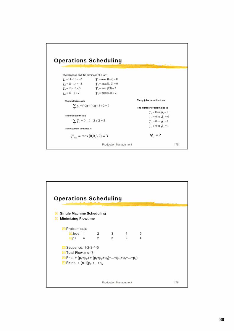
Operations Scheduling
The lateness and the tardiness of a job:
281031013
3141121614
4
3
2
1
=−=
=−=
−=−=
−=−=
LLLL
2}2,0max{3}3,0max{
0}3,0max{0}2,0max{
4
3
2
1
==
==
=−=
=−=
TTTT
The total lateness is
The total tardiness is
The maximum tardiness is
023)3()2( =++−+−=∑i
iL
∑ =+++=i
iT 52300
3}2,3,0,0max{max ==T
Tardy jobs have δi =1, so
The number of tardy jobs is
10100000
44
33
22
11
=⇒>
=⇒>
=⇒=
=⇒=
δδδδ
TTTT
2=NT
Production Management 176
Operations Scheduling
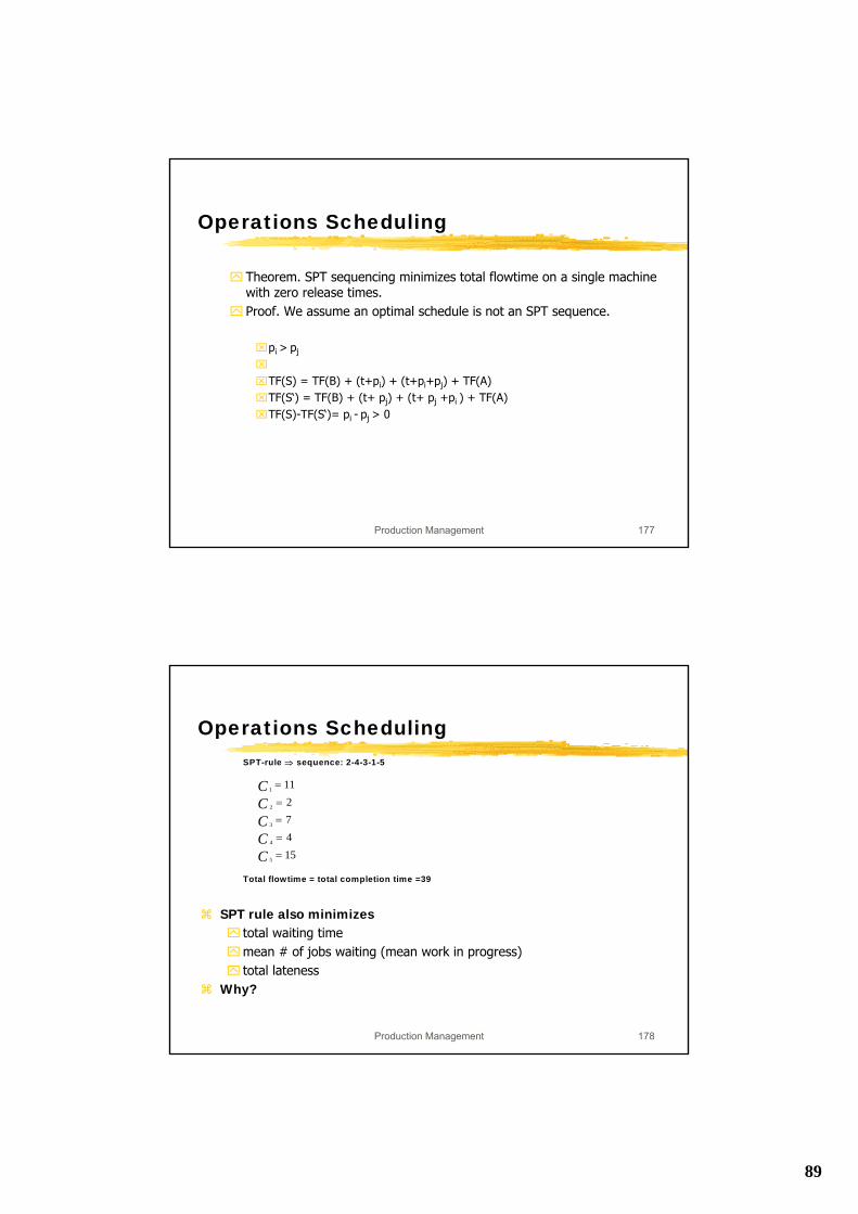
Single Machine SchedulingMinimizing Flowtime
Problem data⌧Job i 1 2 3 4 5⌧p i 4 2 3 2 4
Sequence: 1-2-3-4-5Total Flowtime=?F=p1 + (p1+p2) + (p1+p2+p3)+...+(p1+p2+...+pn)F= np1 + (n-1)p2 +...+pn
89
Production Management 177
Operations Scheduling
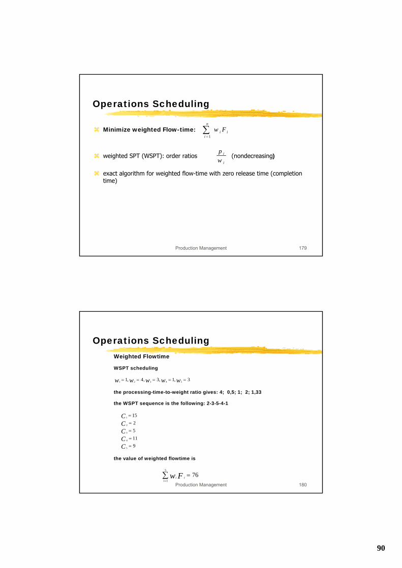
Theorem. SPT sequencing minimizes total flowtime on a single machine with zero release times.Proof. We assume an optimal schedule is not an SPT sequence.
⌧pi > pj
⌧
⌧TF(S) = TF(B) + (t+pi) + (t+pi+pj) + TF(A)⌧TF(S‘) = TF(B) + (t+ pj) + (t+ pj +pi ) + TF(A)⌧TF(S)-TF(S‘)= pi - pj > 0
Production Management 178
SPT-rule ⇒ sequence: 2-4-3-1-5
Total flowtime = total completion time =39
1547211
5
4
3
2
1
=
=
=
=
=
CCCCC
Operations Scheduling
SPT rule also minimizestotal waiting time mean # of jobs waiting (mean work in progress)total lateness
Why?
90
Production Management 179
Operations Scheduling
Minimize weighted Flow-time:
weighted SPT (WSPT): order ratios (nondecreasing)
exact algorithm for weighted flow-time with zero release time (completion time)
∑=
n
iii Fw
1
i
i
wp
Production Management 180
Operations SchedulingWeighted Flowtime
WSPT scheduling
the processing-time-to-weight ratio gives: 4; 0,5; 1; 2; 1,33
the WSPT sequence is the following: 2-3-5-4-1
the value of weighted flowtime is
3,1,3,4,1 54321 ===== wwwww
9115215
5
4
3
2
1
=
=
=
=
=
CCCCC
∑=
=5
176
iii Fw
91
Production Management 181
Operations Scheduling
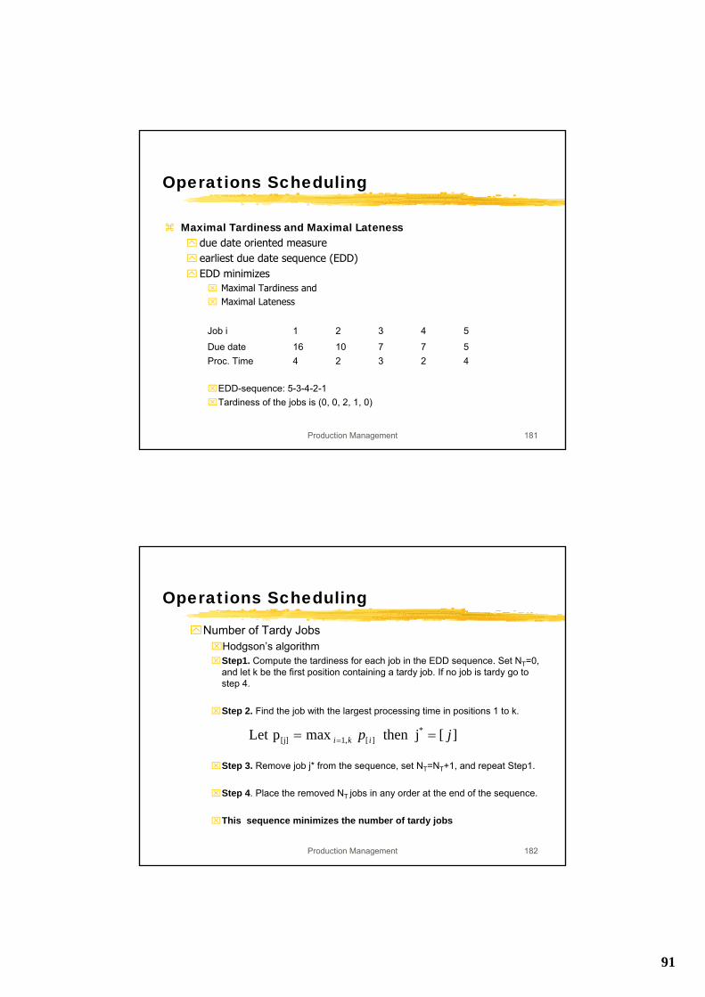
Maximal Tardiness and Maximal Latenessdue date oriented measureearliest due date sequence (EDD)EDD minimizes⌧ Maximal Tardiness and ⌧ Maximal Lateness
Job i 1 2 3 4 5
Due date 16 10 7 7 5Proc. Time 4 2 3 2 4
⌧EDD-sequence: 5-3-4-2-1⌧Tardiness of the jobs is (0, 0, 2, 1, 0)
Production Management 182
Operations Scheduling
Number of Tardy Jobs⌧Hodgson’s algorithm⌧Step1. Compute the tardiness for each job in the EDD sequence. Set NT=0,
and let k be the first position containing a tardy job. If no job is tardy go to step 4.
⌧Step 2. Find the job with the largest processing time in positions 1 to k.
⌧Step 3. Remove job j* from the sequence, set NT=NT+1, and repeat Step1.
⌧Step 4. Place the removed NT jobs in any order at the end of the sequence.
⌧This sequence minimizes the number of tardy jobs
][j then maxpLet *][,1[j] jp iki == =
92
Production Management 183
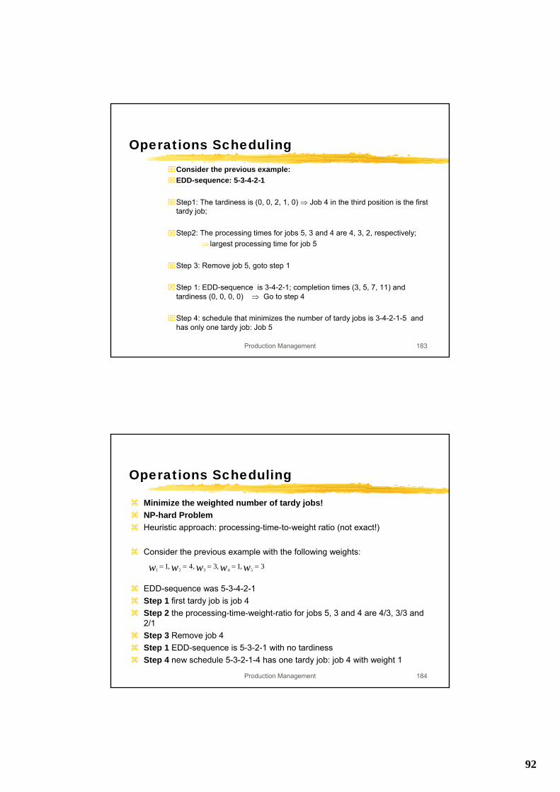
Operations Scheduling⌧Consider the previous example:⌧EDD-sequence: 5-3-4-2-1
⌧Step1: The tardiness is (0, 0, 2, 1, 0) ⇒ Job 4 in the third position is the first tardy job;
⌧Step2: The processing times for jobs 5, 3 and 4 are 4, 3, 2, respectively;⇒ largest processing time for job 5
⌧Step 3: Remove job 5, goto step 1
⌧Step 1: EDD-sequence is 3-4-2-1; completion times (3, 5, 7, 11) and tardiness (0, 0, 0, 0) ⇒ Go to step 4
⌧Step 4: schedule that minimizes the number of tardy jobs is 3-4-2-1-5 and has only one tardy job: Job 5
Production Management 184
Operations Scheduling
Minimize the weighted number of tardy jobs!NP-hard ProblemHeuristic approach: processing-time-to-weight ratio (not exact!)
Consider the previous example with the following weights:
EDD-sequence was 5-3-4-2-1Step 1 first tardy job is job 4Step 2 the processing-time-weight-ratio for jobs 5, 3 and 4 are 4/3, 3/3 and 2/1Step 3 Remove job 4Step 1 EDD-sequence is 5-3-2-1 with no tardinessStep 4 new schedule 5-3-2-1-4 has one tardy job: job 4 with weight 1
3,1,3,4,1 54321 ===== wwwww
93
Production Management 185
Operations Scheduling
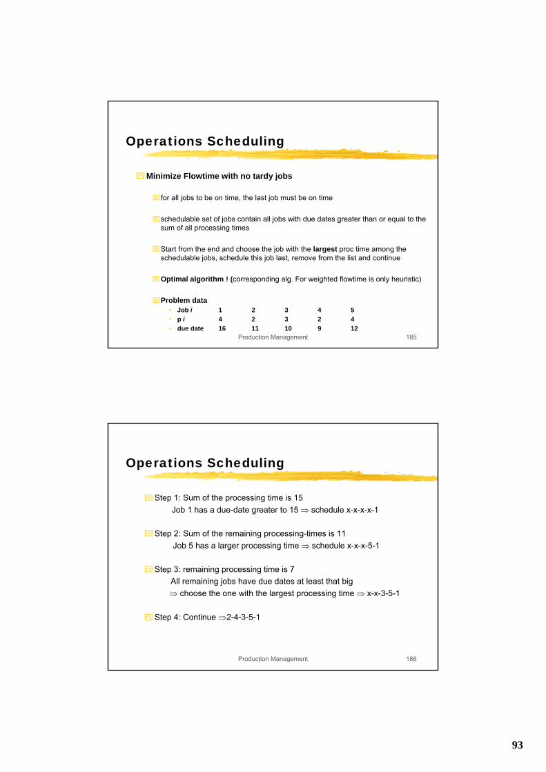
Minimize Flowtime with no tardy jobs
⌧for all jobs to be on time, the last job must be on time
⌧schedulable set of jobs contain all jobs with due dates greater than or equal to the sum of all processing times
⌧Start from the end and choose the job with the largest proc time among the schedulable jobs, schedule this job last, remove from the list and continue
⌧Optimal algorithm ! (corresponding alg. For weighted flowtime is only heuristic)
⌧Problem data• Job i 1 2 3 4 5• p i 4 2 3 2 4• due date 16 11 10 9 12
Production Management 186
Operations Scheduling
Step 1: Sum of the processing time is 15 Job 1 has a due-date greater to 15 ⇒ schedule x-x-x-x-1
Step 2: Sum of the remaining processing-times is 11Job 5 has a larger processing time ⇒ schedule x-x-x-5-1
Step 3: remaining processing time is 7All remaining jobs have due dates at least that big⇒ choose the one with the largest processing time ⇒ x-x-3-5-1
Step 4: Continue ⇒2-4-3-5-1
94
Production Management 187
Operations Scheduling
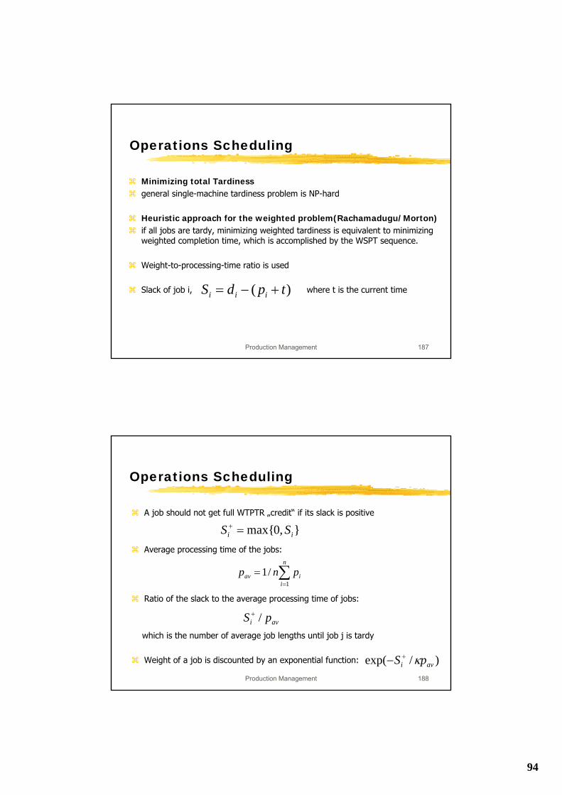
Minimizing total Tardinessgeneral single-machine tardiness problem is NP-hard
Heuristic approach for the weighted problem(Rachamadugu/Morton)if all jobs are tardy, minimizing weighted tardiness is equivalent to minimizing weighted completion time, which is accomplished by the WSPT sequence.
Weight-to-processing-time ratio is used
Slack of job i, where t is the current time)( tpdS iii +−=
Production Management 188
Operations Scheduling
A job should not get full WTPTR „credit“ if its slack is positive
Average processing time of the jobs:
Ratio of the slack to the average processing time of jobs:
which is the number of average job lengths until job j is tardy
Weight of a job is discounted by an exponential function:
},0max{ ii SS =+
∑=
=n
iiav pnp
1/1
avi pS /+
)/exp( avi pS κ+−
95
Production Management 189
Operations Scheduling
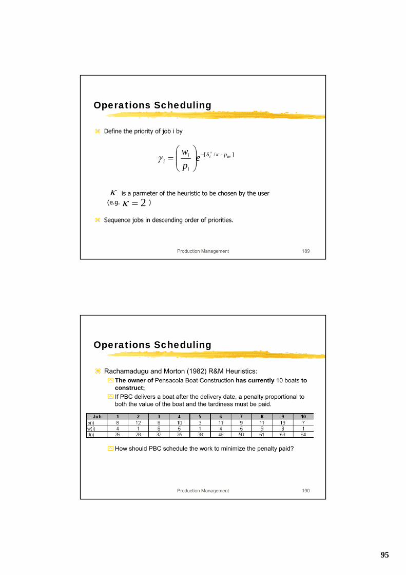
Define the priority of job i by
is a parmeter of the heuristic to be chosen by the user (e.g. )
Sequence jobs in descending order of priorities.
]/[ avi pS
i
ii e
pw ⋅− +
⎟⎟⎠
⎞⎜⎜⎝
⎛= κγ
κ2=κ
Production Management 190
Operations Scheduling
Rachamadugu and Morton (1982) R&M Heuristics:The owner of Pensacola Boat Construction has currently 10 boats to construct;If PBC delivers a boat after the delivery date, a penalty proportional to both the value of the boat and the tardiness must be paid.
How should PBC schedule the work to minimize the penalty paid?
96
Production Management 191
Operations Scheduling
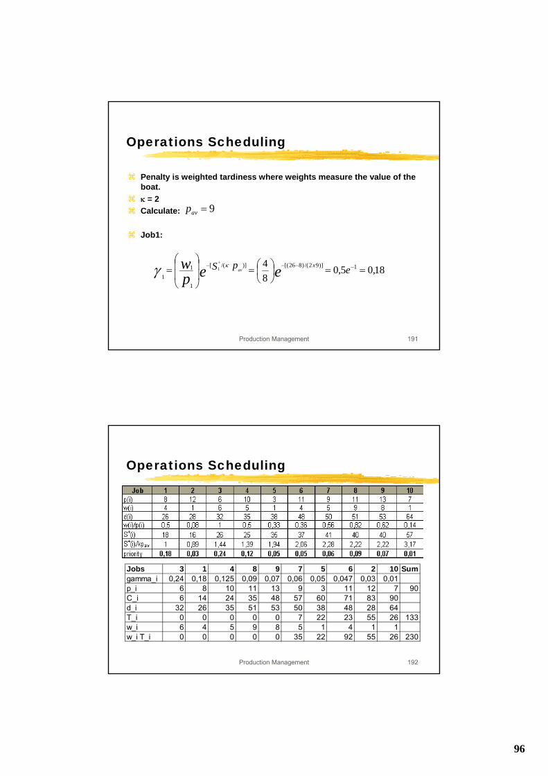
Penalty is weighted tardiness where weights measure the value of the boat.κ = 2Calculate:
Job1:
18,05,084 1)]92/()826[()]/([
1
11
1 ==⎟⎠⎞
⎜⎝⎛=⎟
⎟
⎠
⎞
⎜⎜
⎝
⎛= −−−−
+
epS eepw x
avκγ
9=avp
Production Management 192
Operations Scheduling
Jobs 3 1 4 8 9 7 5 6 2 10 Sumgamma_i 0,24 0,18 0,125 0,09 0,07 0,06 0,05 0,047 0,03 0,01p_i 6 8 10 11 13 9 3 11 12 7 90C_i 6 14 24 35 48 57 60 71 83 90d_i 32 26 35 51 53 50 38 48 28 64T_i 0 0 0 0 0 7 22 23 55 26 133w_i 6 4 5 9 8 5 1 4 1 1w_i T_i 0 0 0 0 0 35 22 92 55 26 230
97
Production Management 193
Operations Scheduling
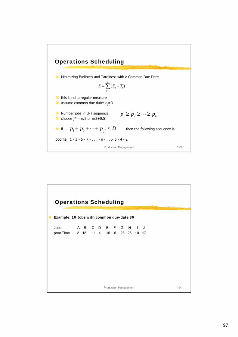
Minimizing Earliness and Tardiness with a Common Due-Date
this is not a regular measureassume common due date: dj=D
Number jobs in LPT sequence: choose j* = n/2 or n/2+0.5
if then the following sequence is
optimal: 1 - 3 - 5 - 7 - . . . - n - . . .- 6 - 4 - 2
∑=
+=n
iii TEZ
1
)(
nppp ≥≥≥ L21
Dppp j ≤+++ *31 L
Production Management 194
Operations Scheduling
Example: 10 Jobs with common due-date 80
Jobs A B C D E F G H I Jproc Time 8 18 11 4 15 5 23 25 10 17
98
Production Management 195
Operations Scheduling
if then apply a heuristic (bySundararaghavan & Ahmed, 1984)
Step 0: Set ; use the LPT sequenceStep 1: If B>A:
assign job k to position bb:=b+1B:=B-pk
elseassign job k to position aa:=a-1A:=A-pk
Step 2: k:=k-1; if k<=n go to step 1.
na ;1 ; ;1
===−== ∑=
n
ii bkDpADB
Dpppj>+++ *31 L
Production Management 196
Operations Scheduling
Problems with non-zero release time
Non-zero release times typically makes scheduling problems much harder, e.g. SPT does in general not minimize total flowtime
Heuristic Approach:At each time t determine the set of schedulable jobs: jobs that have been released but not yet processed.
Choose from the schedulable jobs according to some rule (e.g. SPT for minimizing flowtime)
99
Production Management 197
Operations Scheduling
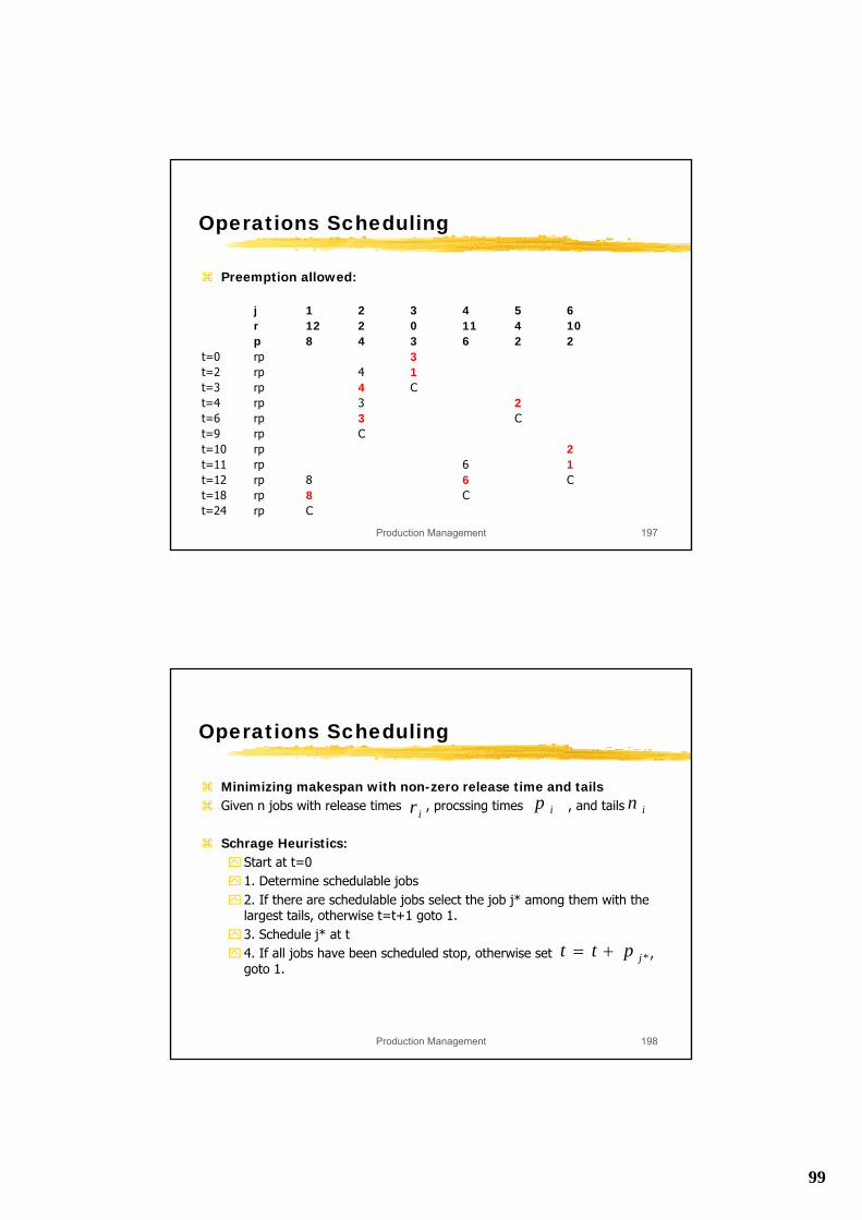
Preemption allowed:
j 1 2 3 4 5 6r 12 2 0 11 4 10p 8 4 3 6 2 2
t=0 rp 3t=2 rp 4 1t=3 rp 4 Ct=4 rp 3 2t=6 rp 3 Ct=9 rp Ct=10 rp 2t=11 rp 6 1t=12 rp 8 6 Ct=18 rp 8 Ct=24 rp C
Production Management 198
Operations Scheduling
Minimizing makespan with non-zero release time and tailsGiven n jobs with release times , procssing times , and tails
Schrage Heuristics:Start at t=01. Determine schedulable jobs2. If there are schedulable jobs select the job j* among them with the largest tails, otherwise t=t+1 goto 1.3. Schedule j* at t4. If all jobs have been scheduled stop, otherwise set , goto 1.
ir ip in
*jptt +=
100
Production Management 199
Operations Scheduling
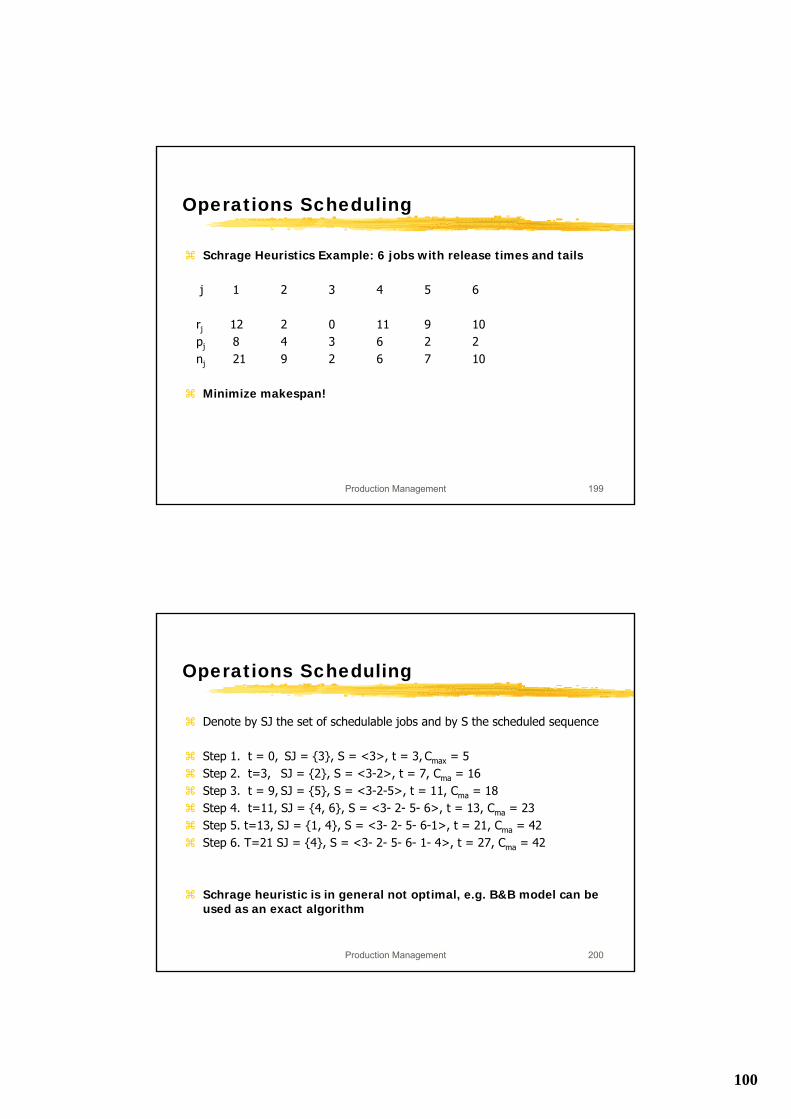
Schrage Heuristics Example: 6 jobs with release times and tails
j 1 2 3 4 5 6
rj 12 2 0 11 9 10pj 8 4 3 6 2 2nj 21 9 2 6 7 10
Minimize makespan!
Production Management 200
Operations Scheduling
Denote by SJ the set of schedulable jobs and by S the scheduled sequence
Step 1. t = 0, SJ = {3}, S = <3>, t = 3, Cmax = 5Step 2. t=3, SJ = {2}, S = <3-2>, t = 7, Cma = 16Step 3. t = 9, SJ = {5}, S = <3-2-5>, t = 11, Cma = 18Step 4. t=11, SJ = {4, 6}, S = <3- 2- 5- 6>, t = 13, Cma = 23Step 5. t=13, SJ = {1, 4}, S = <3- 2- 5- 6-1>, t = 21, Cma = 42Step 6. T=21 SJ = {4}, S = <3- 2- 5- 6- 1- 4>, t = 27, Cma = 42
Schrage heuristic is in general not optimal, e.g. B&B model can be used as an exact algorithm
101
Production Management 201
Operations Scheduling
Minimizing Set-Up Timessequence-dependent set-up timesthe time to change from one product to another may be significant and may depend on the previous part producedpij = time to process job j if it immediately follows job i
Examples:⌧electronics industry⌧paint shops⌧injection molding
minimizes makespanproblem is equivalent to the traveling salesman problem (TSP), which is NP-hard.
Production Management 202
Operations SchedulingSST(=shortest set-up time) heuristic
A metal products manufacturer has contracted to ship metal braces euch day fo four customers.Each brace requires a different set-up on the rolling mill:
Rolling mill set-up timesJob A B C D
A ∞ 3 4 5B 3 ∞ 4 6C 1 6 ∞ 2D 5 4 ∞* ∞
*Job C cannot follow job D, because of quality problems
SST-heuristic:
Step 1 starting arbitrarily by choosing one Job: A
Step 2 B has the smallest set-up time following A; ⇒ A-B
Step 3 C has the smallest set-up time of all the remaining jobs following B; ⇒ A-B-C
Step 4 D is the last remaining job; ⇒ A-B-C-D-A with a makespan of 3 + 4 + 2 + 5 =14
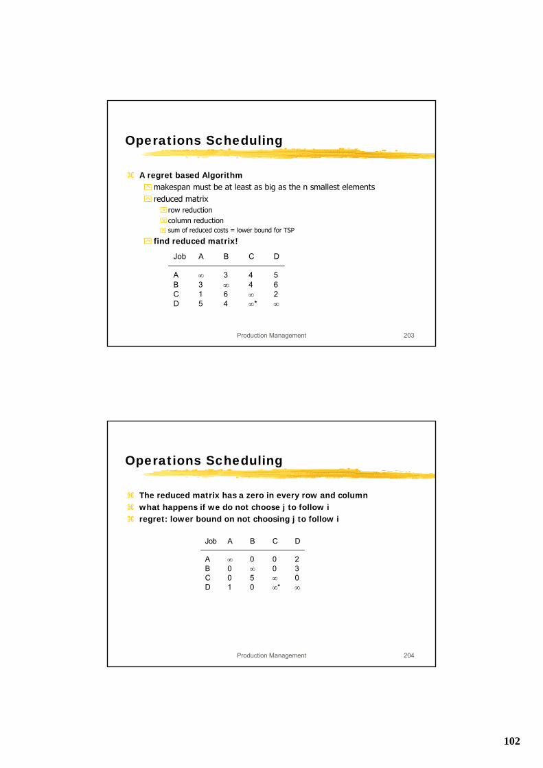
102
Production Management 203
Operations Scheduling
A regret based Algorithmmakespan must be at least as big as the n smallest elementsreduced matrix⌧row reduction⌧column reduction⌧ sum of reduced costs = lower bound for TSP
find reduced matrix!
Job A B C D
A ∞ 3 4 5B 3 ∞ 4 6C 1 6 ∞ 2D 5 4 ∞* ∞
Production Management 204
Operations Scheduling
The reduced matrix has a zero in every row and columnwhat happens if we do not choose j to follow iregret: lower bound on not choosing j to follow i
Job A B C D
A ∞ 0 0 2B 0 ∞ 0 3C 0 5 ∞ 0D 1 0 ∞* ∞
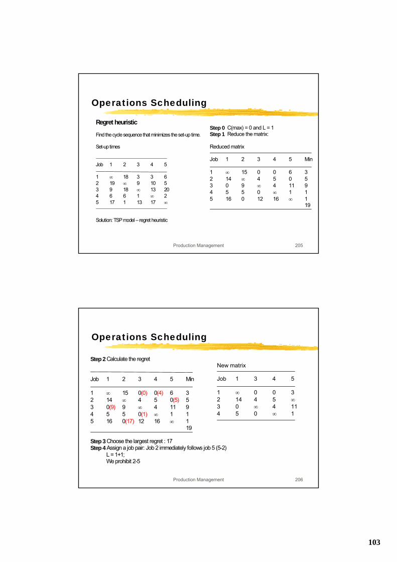
103
Production Management 205
Operations Scheduling
Regret heuristic
Find the cycle sequence that minimizes the set-up time.
Set-up times
Job 1 2 3 4 5
1 ∞ 18 3 3 62 19 ∞ 9 10 53 9 18 ∞ 13 204 6 6 1 ∞ 25 17 1 13 17 ∞
Solution: TSP model – regret heuristic
Step 0 C(max) = 0 and L = 1Step 1 Reduce the matrix:
Reduced matrix
Job 1 2 3 4 5 Min
1 ∞ 15 0 0 6 32 14 ∞ 4 5 0 53 0 9 ∞ 4 11 94 5 5 0 ∞ 1 15 16 0 12 16 ∞ 1
19
Production Management 206
Operations Scheduling
Step 2 Calculate the regret
Job 1 2 3 4 5 Min
1 ∞ 15 0(0) 0(4) 6 32 14 ∞ 4 5 0(5) 53 0(9) 9 ∞ 4 11 94 5 5 0(1) ∞ 1 15 16 0(17) 12 16 ∞ 1
19
Step 3 Choose the largest regret : 17Step 4 Assign a job pair: Job 2 immediately follows job 5 (5-2)
L = 1+1;We prohibit 2-5
New matrix
Job 1 3 4 5
1 ∞ 0 0 32 14 4 5 ∞3 0 ∞ 4 114 5 0 ∞ 1
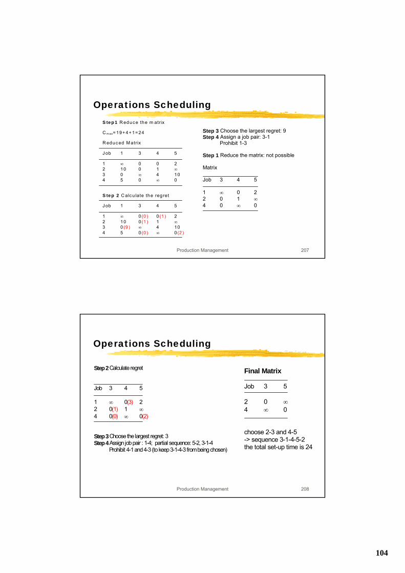
104
Production Management 207
Operations SchedulingS tep 1 R educ e the m atrix C m ax= 19+4+ 1=24 R educ ed M atrix J ob 1 3 4 5 1 ∞ 0 0 2 2 10 0 1 ∞ 3 0 ∞ 4 10 4 5 0 ∞ 0 S tep 2 C alc u late the reg ret J ob 1 3 4 5 1 ∞ 0 (0 ) 0 (1 ) 2 2 10 0 (1 ) 1 ∞ 3 0 (9 ) ∞ 4 10 4 5 0 (0 ) ∞ 0 (2 )
Step 3 Choose the largest regret: 9Step 4 Assign a job pair: 3-1
Prohibit 1-3
Step 1 Reduce the matrix: not possible
Matrix
Job 3 4 5
1 ∞ 0 22 0 1 ∞4 0 ∞ 0
Production Management 208
Operations Scheduling
Step 2 Calculate regret
Job 3 4 5
1 ∞ 0(3) 22 0(1) 1 ∞4 0(0) ∞ 0(2)
Step 3 Choose the largest regret: 3Step 4 Assign job pair : 1-4; partial sequence: 5-2, 3-1-4
Prohibit 4-1 and 4-3 (to keep 3-1-4-3 from being chosen)
Final Matrix
Job 3 5
2 0 ∞4 ∞ 0
choose 2-3 and 4-5-> sequence 3-1-4-5-2the total set-up time is 24
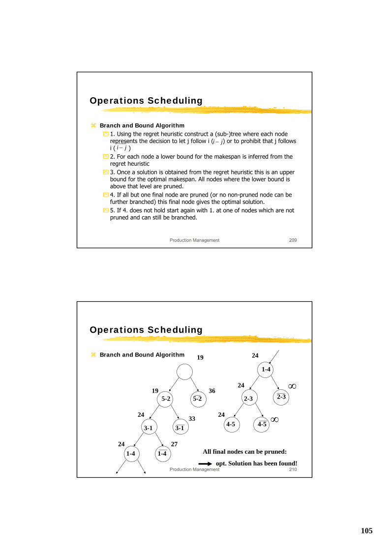
105
Production Management 209
Operations Scheduling
Branch and Bound Algorithm1. Using the regret heuristic construct a (sub-)tree where each node represents the decision to let j follow i ( ) or to prohibit that j follows i ( )2. For each node a lower bound for the makespan is inferred from the regret heuristic3. Once a solution is obtained from the regret heuristic this is an upper bound for the optimal makespan. All nodes where the lower bound is above that level are pruned.4. If all but one final node are pruned (or no non-pruned node can be further branched) this final node gives the optimal solution. 5. If 4. does not hold start again with 1. at one of nodes which are not pruned and can still be branched.
ji −ji −
Production Management 210
Operations Scheduling
Branch and Bound Algorithm
5-2 5-2
3-13-1
1-4 1-4
19
24
24
36
33
27
19
1-4
2-3
4-5 4-5
24
24
2-3
24
∞
∞
All final nodes can be pruned:
opt. Solution has been found!
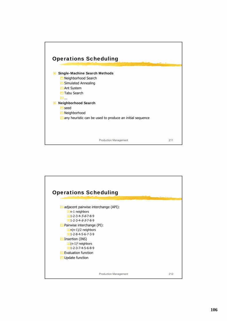
106
Production Management 211
Operations Scheduling
Single-Machine Search MethodsNeighborhood SearchSimulated AnnealingAnt SystemTabu Search...
Neighborhood SearchseedNeighborhoodany heuristic can be used to produce an initial sequence
Production Management 212
Operations Scheduling
adjacent pairwise interchange (API):⌧n-1 neighbors⌧1-2-3-4-5-6-7-8-9⌧1-2-3-4-6-5-7-8-9
Pairwise interchange (PI):⌧n(n-1)/2 neighbors⌧1-2-8-4-5-6-7-3-9
Insertion (INS)⌧(n-1)2 neighbors⌧1-2-3-7-4-5-6-8-9
Evaluation functionUpdate function

107
Production Management 213
Operations SchedulingNeighborhood search
Consider the following single- machine tardiness problem;Use the EDD sequence as the initial seed with an API neighborhood;
Data for neighborhood search
Job 1 2 3 4 5 6
Processing time 10 3 16 8 4 10Due-date 15 16 24 30 35 37
Step 1 Construct the EDD sequence and evaluate its total tardinessSet i = 1 and j = 2
The EDD sequence S*: 1-2-3-4-5-6; tardiness-vector (0, 0 ,5 , 7 , 6, 14)
Production Management 214
Operations Scheduling
Step 2 Swap the jobs in the i-th and j-th position in S*; the sequence is S’with tardiness T’. If T’ < T, go to step4
Step 3 j = j +1: If j >n: go to step 5. Otherwise, i = j-1and go to step 2;
Step 4 Replace S* with S’; i = 1, j = 2; go to step 2
Step 5 Stop; S* is a local optimal sequence.
108
Production Management 215
Operations Scheduling
Neighborhood search solution
Jobs Schedule Tardiness
i j 1 2 3 4 5 6 32
1 2 2 1 3 4 5 6 322 3 1 3 2 4 5 6 423 4 1 2 4 3 5 6 334 5 1 2 3 5 4 6 30
1 2 2 1 3 5 4 6 302 3 1 3 2 5 4 6 403 5 1 2 5 3 4 6 345 4 1 2 3 4 5 6 324 6 1 2 3 5 6 4 32
Production Management 216
Operations Scheduling
Single machine resultsFlowtime - SPT (E)Lateness - SPT (E)Weighted Flowtime -WSPT (E)Maximal Tardiness (Lateness) - EDD (E)Nb. Of tardy jobs - Hodgson (E)weighted nb. Of tardy jobs - modified Hodgson (H)No jobs tardy/flowtime - modified SPT (E)Tardiness - R&M (H)weighted Tardiness - R&M (H)makespan with non-zero release time and tails - Schrage (H)Sequence dependent - SST (H), regret (H), B&B (E)
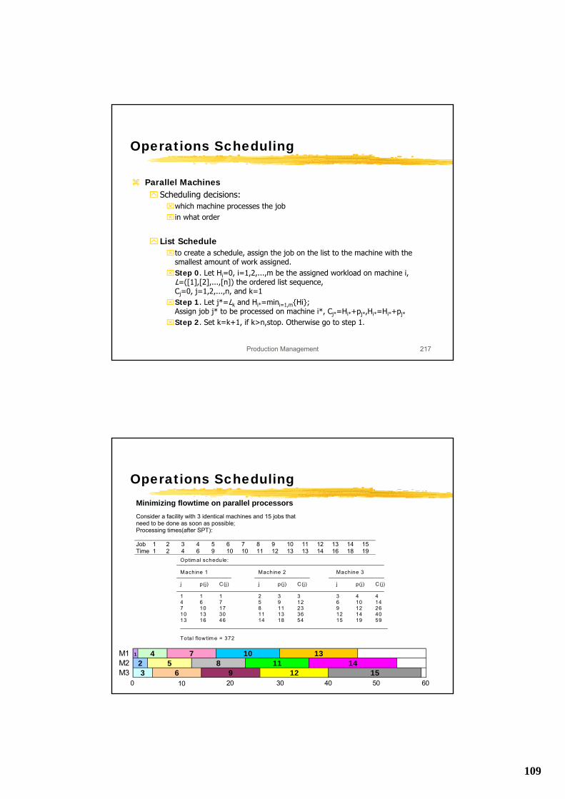
109
Production Management 217
Operations Scheduling
Parallel MachinesScheduling decisions:⌧which machine processes the job⌧in what order
List Schedule⌧to create a schedule, assign the job on the list to the machine with the
smallest amount of work assigned.⌧Step 0. Let Hi=0, i=1,2,...,m be the assigned workload on machine i,
L=([1],[2],...,[n]) the ordered list sequence, Cj=0, j=1,2,...,n, and k=1
⌧Step 1. Let j*=Lk and Hi*=mini=1,m{Hi};Assign job j* to be processed on machine i*, Cj*=Hi*+pj*,Hi*=Hi*+pj*
⌧Step 2. Set k=k+1, if k>n,stop. Otherwise go to step 1.
Production Management 218
Operations SchedulingMinimizing flowtime on parallel processorsConsider a facility with 3 identical machines and 15 jobs thatneed to be done as soon as possible;Processing times(after SPT):
Job 1 2 3 4 5 6 7 8 9 10 11 12 13 14 15Time 1 2 4 6 9 10 10 11 12 13 13 14 16 18 19
Optim al schedule:
Machine 1 Machine 2 Machine 3
j p(j) C(j) j p(j) C(j) j p(j) C(j)
1 1 1 2 3 3 3 4 44 6 7 5 9 12 6 10 147 10 17 8 11 23 9 12 2610 13 30 11 13 36 12 14 4013 16 46 14 18 54 15 19 59
Total flowtim e = 372
M1 1
M2M3 12
1314
1523
45
6
78
9
1011
0 10 20 30 40 50 60
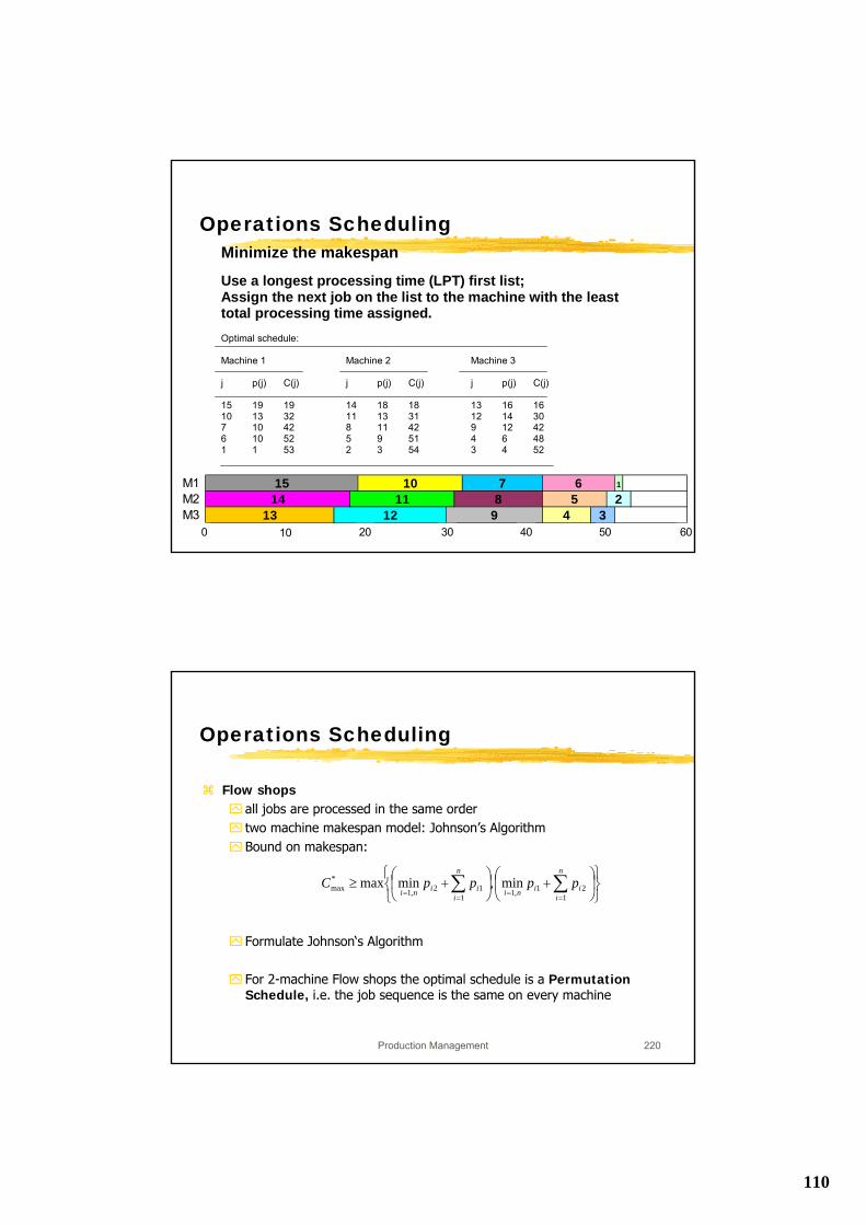
110
Production Management 219
Operations SchedulingMinimize the makespan Use a longest processing time (LPT) first list; Assign the next job on the list to the machine with the least total processing time assigned. Optimal schedule: Machine 1 Machine 2 Machine 3 j p(j) C(j) j p(j) C(j) j p(j) C(j) 15 19 19 14 18 18 13 16 16 10 13 32 11 13 31 12 14 30 7 10 42 8 11 42 9 12 42 6 10 52 5 9 51 4 6 48 1 1 53 2 3 54 3 4 52
M1 1
M2M3
23
1514
13
1011
128
9
7 65
40 10 20 30 40 50 60
Production Management 220
Operations Scheduling
Flow shopsall jobs are processed in the same ordertwo machine makespan model: Johnson’s AlgorithmBound on makespan:
Formulate Johnson‘s Algorithm
For 2-machine Flow shops the optimal schedule is a Permutation Schedule, i.e. the job sequence is the same on every machine
⎭⎬⎫
⎩⎨⎧
⎟⎠
⎞⎜⎝
⎛+⎟
⎠
⎞⎜⎝
⎛+≥ ∑∑
==
==
n
iiini
n
iiini
ppppC1
21,1112,1
*max min,minmax
111
Production Management 221
Operations Scheduling
Makespan with more than two machinesJohnson‘s algorithm will work in special cases, e.g. three machineproblem where the second machine is dominated:
Formulate an artificial two machine problem with
and solve it using the Johnson algorithm gives the optimal solutionfor the three machine problem
)min,max(min 312 iii ppp ≤
322i211 and p iiiii ppppp +=′+=′
Production Management 222
Operations Scheduling
Heuristics for the m-machine problemCambell, Dudek and Smith (1970)convert a m-machine problem into a two machine problemhow?
Start with:k=1 and l=m; then k=2 and l=m-1; until: k=m-1 and l=2m-1 schedules are generatedUse the best of these m-1 schedules
∑∑==
=′=′m
ljiji
k
jiji pppp 2
11 and
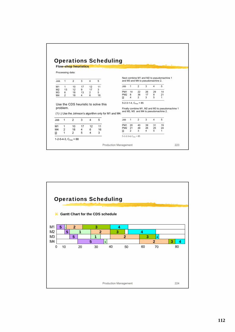
112
Production Management 223
Operations SchedulingFlow-shop heuristics
Processing data:
Job 1 2 3 4 5
M1 1 10 17 12 11M2 13 12 9 17 3M3 6 18 13 2 5M4 2 18 4 6 16
Use the CDS heuristic to solve thisproblem.
(1) i.) Use the Johnson’s algorithm only for M1 and M4:
Job 1 2 3 4 5
M1 1 10 17 12 11M4 2 18 4 6 16[j] 1 2 5 4 3
1-2-5-4-3, Cmax = 88
Next combine M1 and M2 to pseudomachine 1 and M3 and M4 to pseudomachine 2. Job 1 2 3 4 5 PM1 14 22 26 29 14 PM2 8 36 17 8 21 [j] 4 2 3 5 1 5-2-3-1-4, Cmax = 85 Finally combine M1, M2 and M3 to pseudomachine 1 and M2, M3 and M4 to pseudomachine 2. Job 1 2 3 4 5 PM1 20 40 39 31 19 PM2 21 48 26 25 24 [j] 2 3 4 5 1 5-1-2-3-4, Cmax = 85
Production Management 224
Operations Scheduling
Gantt Chart for the CDS schedule
M1 1
M2M3M4 3 4
4
5 1 25 1 2
2 3 45 1 2 3
54
3
0 10 20 30 40 50 60 70 80
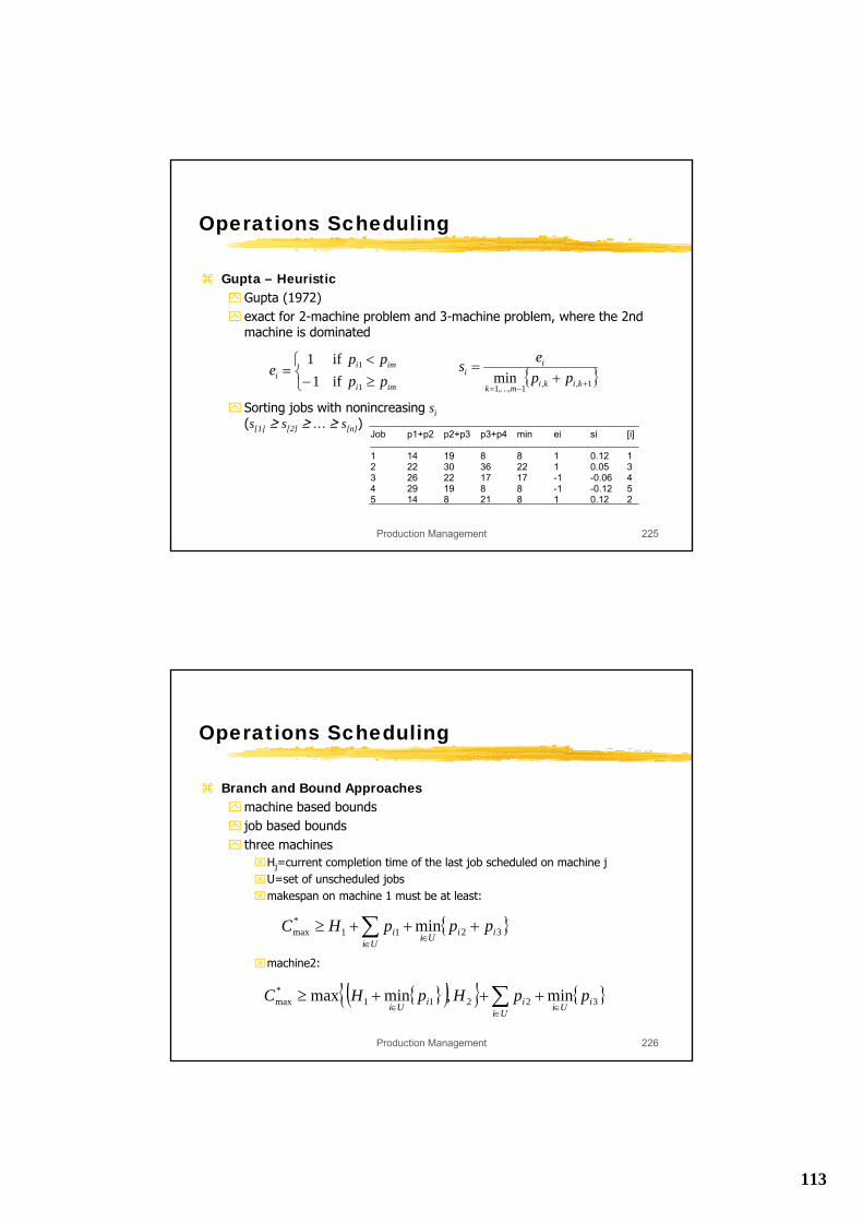
113
Production Management 225
Operations Scheduling
Gupta – HeuristicGupta (1972)exact for 2-machine problem and 3-machine problem, where the 2nd machine is dominated
Sorting jobs with nonincreasing si(s[1] ≥ s[2] ≥ … ≥ s[n])
⎩⎨⎧
≥−<
=imi
imii pp
ppe
1
1
if1 if1
{ }1,,1,,1min +−=
+=
kikimk
ii pp
esK
Job p1+p2 p2+p3 p3+p4 min ei si [i] 1 14 19 8 8 1 0.12 1 2 22 30 36 22 1 0.05 3 3 26 22 17 17 -1 -0.06 4 4 29 19 8 8 -1 -0.12 5 5 14 8 21 8 1 0.12 2
Production Management 226
Operations Scheduling
Branch and Bound Approachesmachine based boundsjob based boundsthree machines⌧Hj=current completion time of the last job scheduled on machine j⌧U=set of unscheduled jobs⌧makespan on machine 1 must be at least:
⌧machine2:
{ }3211*max min iiUiUi
i pppHC +++≥∈
∈∑
{ }( ){ } { }∑∈
∈∈+++≥
UiiUiiiUi
ppHpHC 32211*max min,minmax
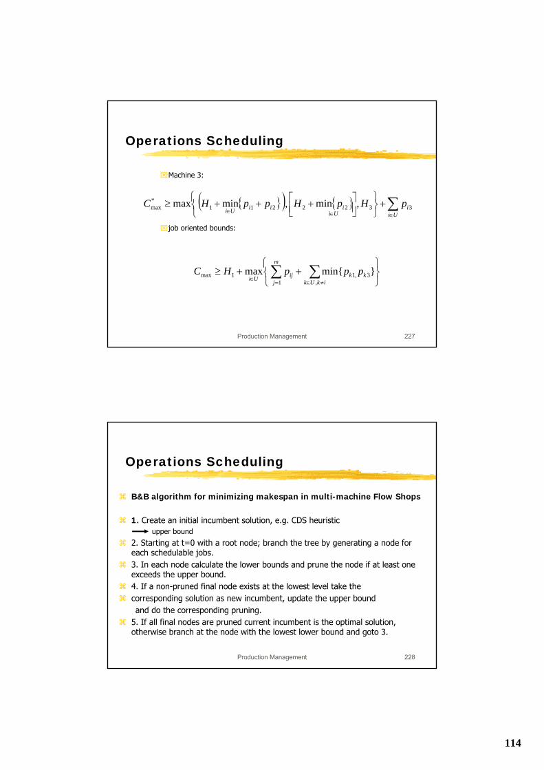
114
Production Management 227
Operations Scheduling
⌧Machine 3:
⌧job oriented bounds:
{ }( ) { } ∑∈∈∈
+⎭⎬⎫
⎩⎨⎧
⎥⎦⎤
⎢⎣⎡ +++≥
Uii
UiiiiUi
pHpHppHC 3322211*max ,min,minmax
⎭⎬⎫
⎩⎨⎧
++≥ ∑∑≠∈=
∈ ikUkkk
m
jijUi
pppHC,
3,11
1max }min{max
Production Management 228
Operations Scheduling
B&B algorithm for minimizing makespan in multi-machine Flow Shops
1. Create an initial incumbent solution, e.g. CDS heuristicupper bound
2. Starting at t=0 with a root node; branch the tree by generating a node foreach schedulable jobs.3. In each node calculate the lower bounds and prune the node if at least oneexceeds the upper bound.4. If a non-pruned final node exists at the lowest level take thecorresponding solution as new incumbent, update the upper boundand do the corresponding pruning.
5. If all final nodes are pruned current incumbent is the optimal solution, otherwise branch at the node with the lowest lower bound and goto 3.
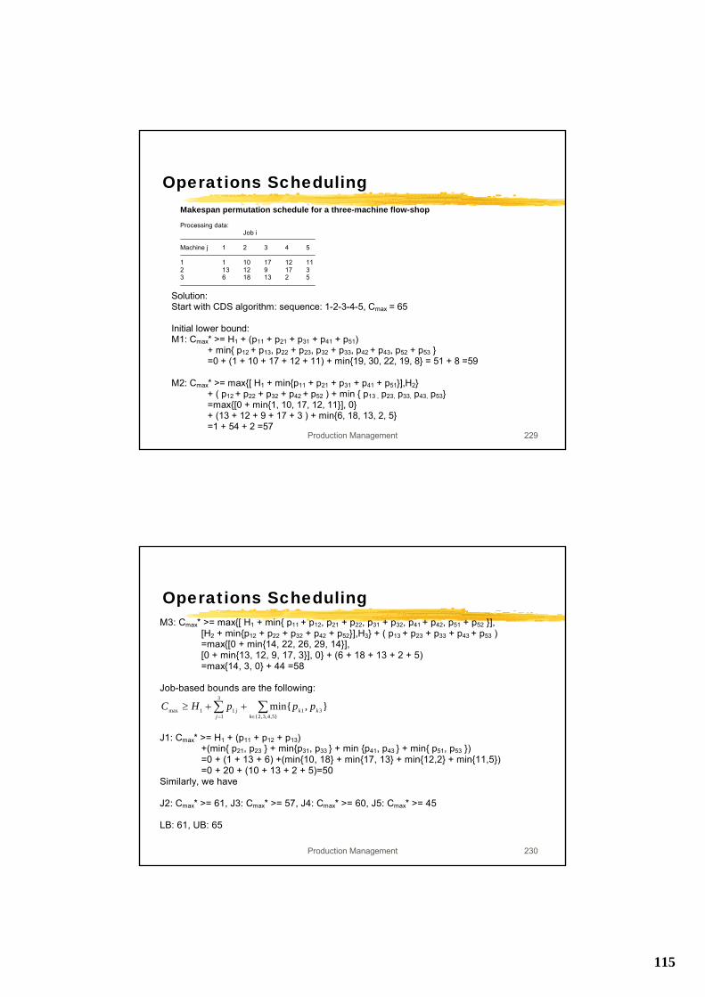
115
Production Management 229
Operations SchedulingMakespan permutation schedule for a three-machine flow-shop
Processing data:Job i
Machine j 1 2 3 4 5
1 1 10 17 12 112 13 12 9 17 33 6 18 13 2 5
Solution: Start with CDS algorithm: sequence: 1-2-3-4-5, Cmax = 65 Initial lower bound: M1: Cmax* >= H1 + (p11 + p21 + p31 + p41 + p51) + min{ p12 + p13, p22 + p23, p32 + p33, p42 + p43, p52 + p53 } =0 + (1 + 10 + 17 + 12 + 11) + min{19, 30, 22, 19, 8} = 51 + 8 =59 M2: Cmax* >= max{[ H1 + min{p11 + p21 + p31 + p41 + p51}],H2} + ( p12 + p22 + p32 + p42 + p52 ) + min { p13 , p23, p33, p43, p53} =max{[0 + min{1, 10, 17, 12, 11}], 0} + (13 + 12 + 9 + 17 + 3 ) + min{6, 18, 13, 2, 5} =1 + 54 + 2 =57
Production Management 230
Operations SchedulingM3: Cmax* >= max{[ H1 + min{ p11 + p12, p21 + p22, p31 + p32, p41 + p42, p51 + p52 }], [H2 + min{p12 + p22 + p32 + p42 + p52}],H3} + ( p13 + p23 + p33 + p43 + p53 ) =max{[0 + min{14, 22, 26, 29, 14}], [0 + min{13, 12, 9, 17, 3}], 0} + (6 + 18 + 13 + 2 + 5) =max{14, 3, 0} + 44 =58 Job-based bounds are the following:
J1: Cmax* >= H1 + (p11 + p12 + p13) +(min{ p21, p23 } + min{p31, p33 } + min {p41, p43 } + min{ p51, p53 }) =0 + (1 + 13 + 6) +(min{10, 18} + min{17, 13} + min{12,2} + min{11,5}) =0 + 20 + (10 + 13 + 2 + 5)=50 Similarly, we have J2: Cmax* >= 61, J3: Cmax* >= 57, J4: Cmax* >= 60, J5: Cmax* >= 45 LB: 61, UB: 65
∑∑∈=
++≥}5,4,3,2{
31
3
111max },min{
kkk
jj pppHC
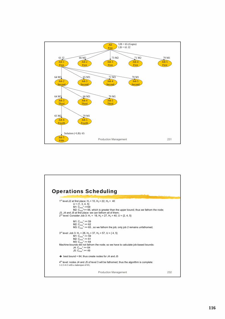
116
Production Management 231
AllFree
UB = 65 (Gupta)LB = 61 J2
Job 1First
Job 2First
Job 3First
Job 4First
Job 5First
61 J2 66 M2 73 M2 71 M2 70 M1
Job 2Second
Job 3Second
Job 4Second
Job 5Second
64 M3 65 M3 72 M3 70 M1
Job 3Third
Job 4Third
Job 5Third
64 M3 66 M3 70 M1
Job 4Fourth
Job 5Fourth
65 M2 70 M1
Job 5Fifth
Solution (=LB): 65
Production Management 232
Operations Scheduling1st level:J2 at first place: H1 = 10, H2 = 22, H3 = 40
U = {1, 3, 4, 5}M1: Cmax* >=59M2: Cmax*>= 66, which is greater than the upper bound; thus we fathom the node;
J3, J4 and J5 at first place: we can fathom all of them;2nd level: Consider Job 3: H1 = 18, H2 = 27, H3 = 40, U = {2, 4, 5}
M1: Cmax* >= 59M2: Cmax* >= 62M3: Cmax* >= 65 , so we fathom the job; only job 2 remains unfathomed;
3rd level: Job 3: H1 = 28, H2 = 37, H3 = 57, U = { 4, 5}M1: Cmax* >= 59M2: Cmax* >= 61M3: Cmax* >= 64
Machine-bounds did not fathom the node; so we have to calculate job-based bounds:J4: Cmax* >= 64J5: Cmax* >= 49
best bound = 64; thus create nodes for J4 and J5
4th level: nodes J4 and J5 of level 3 will be fathomed; thus the algorithm is complete:1-2-3-4-5 with a makespan of 65;
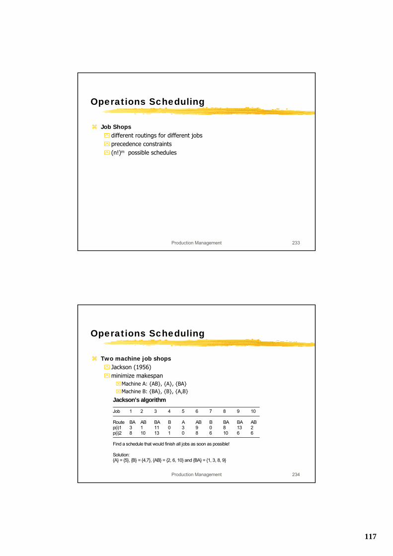
117
Production Management 233
Operations Scheduling
Job Shopsdifferent routings for different jobsprecedence constraints(n!)m possible schedules
Production Management 234
Operations Scheduling
Two machine job shopsJackson (1956)minimize makespan⌧Machine A: {AB}, {A}, {BA}⌧Machine B: {BA}, {B}, {A,B}
Jackson’s algorithm
Job 1 2 3 4 5 6 7 8 9 10
Route BA AB BA B A AB B BA BA ABp(i)1 3 1 11 0 3 9 0 8 13 2p(i)2 8 10 13 1 0 8 6 10 6 6
Find a schedule that would finish all jobs as soon as possible!
Solution:{A} = {5}, {B} = {4,7}, {AB} = {2, 6, 10} and {BA} = {1, 3, 8, 9}
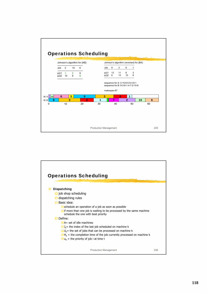
118
Production Management 235
Operations SchedulingJohnson’s algorithm for {AB}:
Job 2 10 6
p(i)1 1 2 9p(i)2 10 6 8
Johnson’s algorithm (reversed) for {BA}:
Job 9 3 8 1
p(i)1 13 11 8 3p(i)2 6 13 10 8
sequence for A: 2-10-6-5-9-3-8-1sequence for B: 9-3-8-1-4-7-2-10-6
makespan:67
M: A
M: B 2 10 69 3 8 110 6 5 9 3 8 1
70 10 20 30 40 50 60
Production Management 236
Operations Scheduling
Dispatchingjob shop schedulingdispatching rulesBasic idea:⌧schedule an operation of a job as soon as possible⌧if more than one job is waiting to be processed by the same machine
schedule the one with best priority
Define:⌧A= set of idle machines⌧Jk= the index of the last job scheduled on machine k⌧Uk= the set of jobs that can be processed on machine k⌧Hk = the completion time of the job currently processed on machine k⌧uit = the priority of job i at time t
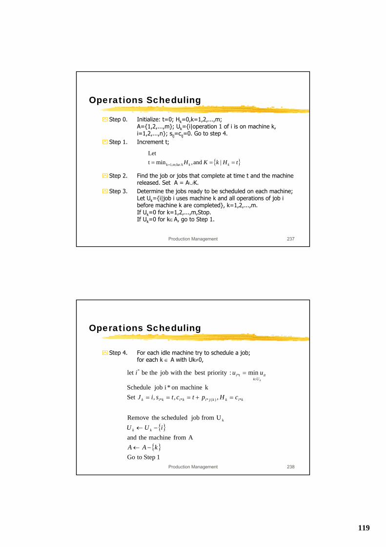
119
Production Management 237
Operations Scheduling
Step 0. Initialize: t=0; Hk=0,k=1,2,...,m;A={1,2,...,m}; Uk={i|operation 1 of i is on machine k, i=1,2,...,n}; sij=cij=0. Go to step 4.
Step 1. Increment t;
Step 2. Find the job or jobs that complete at time t and the machine released. Set A = A∪K.
Step 3. Determine the jobs ready to be scheduled on each machine;Let Uk={i|job i uses machine k and all operations of job i before machine k are completed}, k=1,2,...,m.If Uk=0 for k=1,2,...,m,Stop.If Uk=0 for k∈A, go to Step 1.
{ }tHkKH kk === ∉= | and,mintLet
Akm;1,k
Production Management 238
Operations Scheduling
Step 4. For each idle machine try to schedule a job;for each k ∈ A with Uk≠0,
{}
{ }1 Step toGo
A from machine theand
Ufrom job scheduled theRemove
,,,Set k machineon *i job Schedule
min:prioritybest with thejob thebe let
k
*)(***
*
kAA
iUU
cHptctsiJ
uui
kk
kikkjikikik
Uiiti*t
k
−←
−←
=+===
=∈
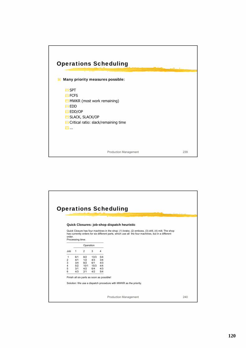
120
Production Management 239
Operations Scheduling
Many priority measures possible:
SPTFCFSMWKR (most work remaining)EDDEDD/OPSLACK, SLACK/OPCritical ratio: slack/remaining time...
Production Management 240
Operations Scheduling
Quick Closures: job-shop dispatch heuristic
Quick Closure has four machines in the shop: (1) brake, (2) emboss, (3) drill, (4) mill; The shophas currently orders for six different parts, which use all the four machines, but in a differentorder.Processing time:
Operation
Job 1 2 3 4
1 6/1 8/2 13/3 5/42 4/1 1/2 4/3 3/43 3/4 8/2 6/1 4/34 5/2 10/1 15/3 4/45 3/1 4/2 6/4 4/36 4/3 2/1 4/2 5/4
Finish all six parts as soon as possible!
Solution: We use a dispatch procedure with MWKR as the priority.
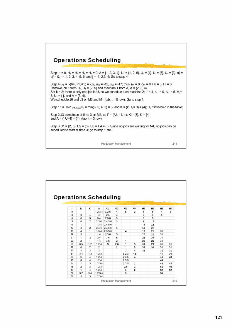
121
Production Management 241
Operations Scheduling
Step1 t = 0, H1 = H2 = H3 = H4 = 0, A = {1, 2, 3, 4}, U1 = {1, 2, 5}, U2 = {4}, U3 = {6}, U4 = {3}; sij = cij = 0, i = 1, 2, 3, 4, 5, 6; and j = 1, 2,3, 4; Go to step 4 Step 4 u10 = -(6+8+13+5) = -32, u20 = -12, u50 = -17; thus s11 = 0, c11 = 0 + 6 = 6, H1 = 6. Remove job 1 from U1, U1 = {2, 5} and machine 1 from A, A = {2, 3, 4}. Set k = 2; there is only one job in U2 so we schedule it on machine 2; i* = 4, s41 = 0, c41 = 5, H2= 5, U2 = { }, and A = {3, 4}. We schedule J6 and J3 on M3 and M4 (tab: t = 0 row). Go to step 1. Step 1 t = min k=1,m:kεAHk = min{6, 5, 4, 3} = 3, and K = {k\Hk = 3} = {4}; Hk min is bold in the table; Step 2 J3 completes at time 3 on M4, so i3 = {i\Jk = i, k ε K} ={3}, K = {4}, and A = {} U {4} = {4}, (tab: t = 3 row) Step 3 U1 = {2, 5}, U2 = {3}, U3 = U4 = { }; Since no jobs are waiting for M4, no jobs can be scheduled to start at time 3; go to step 1 etc.
Production Management 242
Operations Scheduling
t it K A U1 U2 U3 U4 H1 H2 H3 H40 - - 1,2,3,4 1,2,5 4 6 3 6 5 4 33 3 4 4 2,5 3 6 5 44 6 3 3,4 2,5,6 3 6 55 4 2 2,3,4 2,4,5,6 3 6 136 1 1 1,3,4 2,4,5,6 1 16 13
13 3 2 2,3,4 2,3,5,6 1 16 2116 4 1 1,3,4 2,3,5,6 4 19 21 3119 5 1 1,4 2,3,6 5 23 21 3121 1 2 2,4 3,6 5 1 23 25 3123 2 1 1,4 3,6 2 1 25 25 3125 6,5 1,2 1,2,4 3 2,6 1 5 31 29 31 3129 6 2 2 2 1 6 31 30 31 3130 2 2 2 1,2 6 31 31 3131 3,4 1,3 1,2,3 1,2,3 4,6 44 3636 6 4 1,2,4 2,3,5 4 44 4040 4 4 1,2,4 2,3,5 4444 1 3 1,2,3,4 2,3,5 1 48 4948 2 3 1,2,3 3,5 2 52 4949 1 4 1,2,4 5 2 52 5252 3,2 3,4 1,2,3,4 5 5656 5 3 1,2,3,4
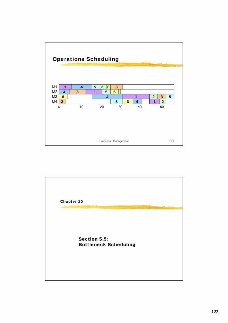
122
Production Management 243
Operations Scheduling
M1M2 2
M3M4 6 4 1 2
33 1 5 6
1 5 2 64463
45
1 2 3 5
0 10 20 30 40 50
Chapter 10
Section 5.5: Bottleneck Scheduling
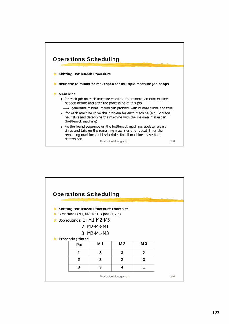
123
Production Management 245
Operations Scheduling
Shifting Bottleneck Procedure
heuristic to minimize makespan for multiple machine job shops
Main idea:1. for each job on each machine calculate the minimal amount of time
needed before and after the processing of this job generates minimal makespan problem with release times and tails
2. for each machine solve this problem for each machine (e.g. Schrage heuristic) and determine the machine with the maximal makespan(bottleneck machine)
3. Fix the found sequence on the bottleneck machine, update release times and tails on the remaining machines and repeat 2. for the remaining machines until schedules for all machines have been determined
Production Management 246
Operations Scheduling
Shifting Bottleneck Procedure Example:3 machines (M1, M2, M3), 3 jobs (1,2,3)
Job routings: 1: M1-M2-M32: M2-M3-M13: M2-M1-M3
Processing times:pik M1 M2 M3
1 3 3 2
2 3 2 3
3 3 4 1
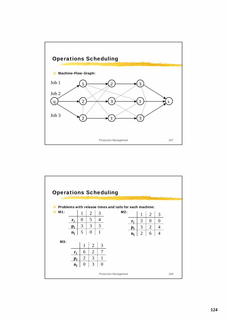
124
Production Management 247
Operations Scheduling
Machine-Flow-Graph:
2
2
1
3
1
2
3
3
sq 1
Job 1
Job 2
Job 3
Production Management 248
Operations Scheduling
Problems with release times and tails for each machine:M1: M2:
M3:
1 2 3rj 0 5 4pj 3 3 3nj 5 0 1
1 2 3rj 3 0 0pj 3 2 4nj 2 6 4
1 2 3rj 6 2 7pj 2 3 1nj 0 3 0
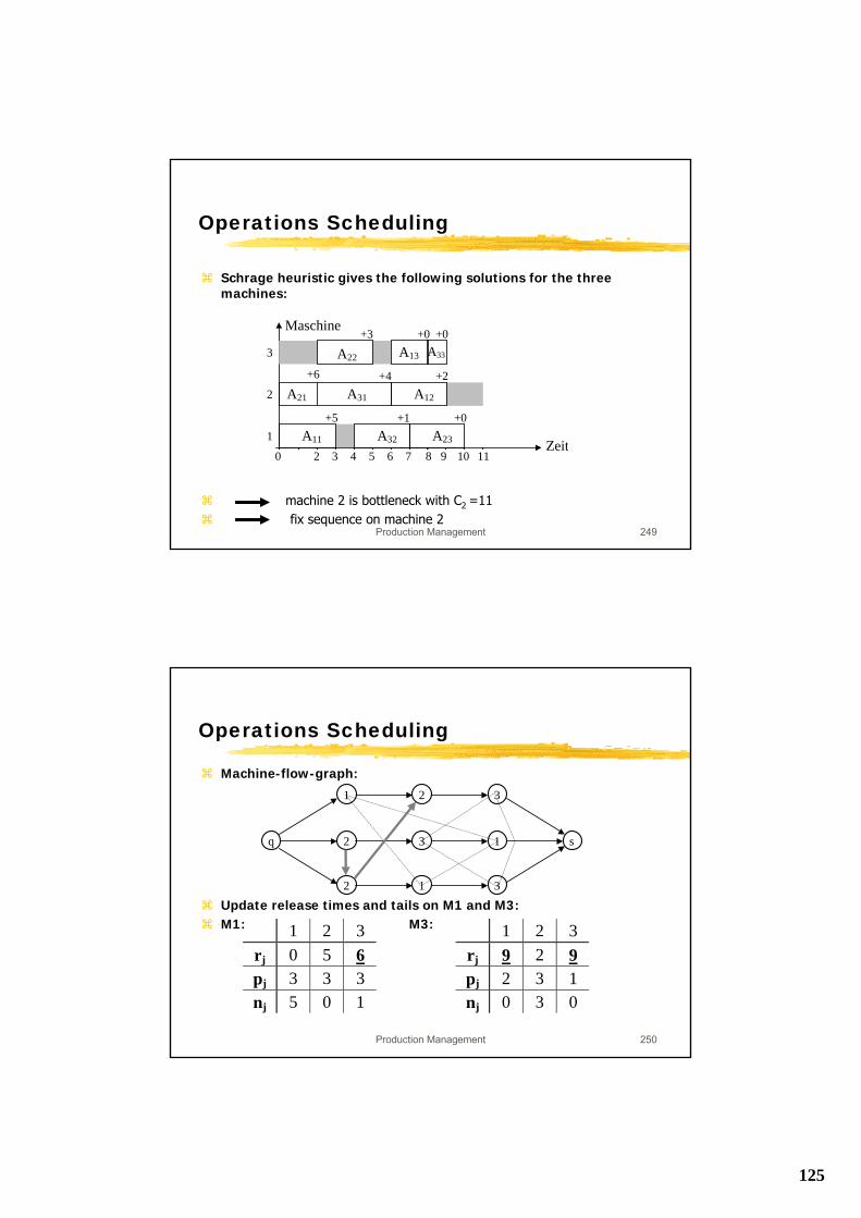
125
Production Management 249
Operations Scheduling
Schrage heuristic gives the following solutions for the three machines:
machine 2 is bottleneck with C2 =11fix sequence on machine 2
A31 A12
Maschine
11109654
+2+4+6
2
320Zeit
A21
87
A32 A23
+0+1+51 A11
A33A13
+0+0+33 A22
Production Management 250
Operations Scheduling
Machine-flow-graph:
Update release times and tails on M1 and M3:M1: M3:
2
2
1
3
1
2
3
3
sq 1
1 2 3rj 0 5 6pj 3 3 3nj 5 0 1
1 2 3rj 9 2 9pj 2 3 1nj 0 3 0
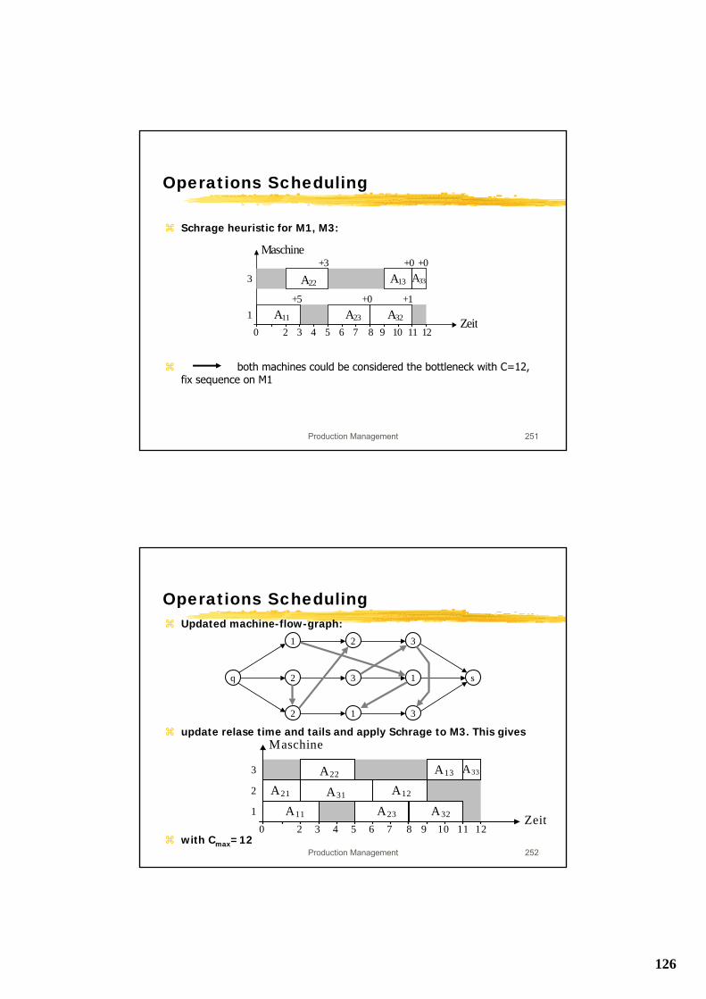
126
Production Management 251
Operations Scheduling
Schrage heuristic for M1, M3:
both machines could be considered the bottleneck with C=12, fix sequence on M1
3
Maschine
11109654320Zeit
87
A32A23
+0 +1+51 A11
A33A13
+0+0+3
A22
12
Production Management 252
Operations SchedulingUpdated machine-flow-graph:
update relase time and tails and apply Schrage to M3. This gives
with Cmax=12
2
2
1
3
1
2
3
3
sq 1
3
Maschine
11109654320Zeit
87
A32A231 A11
A33A13A22
12
2 A12A21 A31
127
Production Management 253
Operations Scheduling
Finite Capacity Scheduling
⌧MRP systems generally assume constant lead times, ignore setups
⌧MRP plans might be unrealistic
⌧Traditionally problem hiden by inventory and excess capacity
⌧Reducing Inventory and capacity makes finite capacity scheduling crucial
⌧Computer-assisted finitie capacity scheduling systems rather than manualscheduling by foreman
Production Management 254
Operations Scheduling
Work to do: 8.3abcde, 8.4, 8.5, 8.6, 8.10, 8.14, 8.16, 8.18 (with the following due dates: 42, 50, 12, 63, 23, 34, 36, 42, 54, 32)8.30ab, 8.32abc, 8.36ab, 8.43, 8.44, 8.49ab, 8.51ab, 8.56, 8.57 (apply shifting bottleneck procedure)
Minicase: Ilana Designs