Chapter 1-7 Goodness of Fit Testing Reliability · 6s ANALYZE Belt Expected Value The expected value is the probability of an event times the sample size. The probability of finding

6s

ANALYZE Le

an S

ix S

igm

a B

lack

Be

lt

Chapter 1-7

Goodness of Fit Testing Reliability

© 2014 Institute of Industrial Engineers 1-7-1

6s

ANALYZE Le

an S

ix S

igm

a B

lack

Be

lt

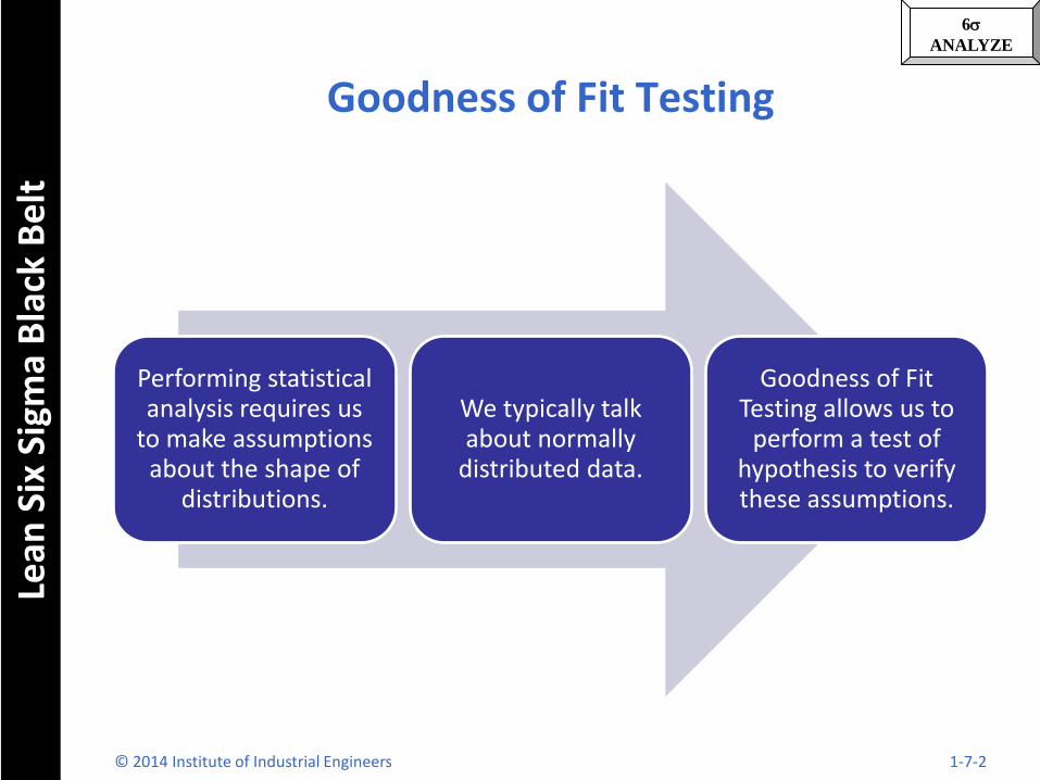
Goodness of Fit Testing

Performing statistical analysis requires us

to make assumptions about the shape of

distributions.

We typically talk about normally

distributed data.

Goodness of Fit Testing allows us to

perform a test of hypothesis to verify these assumptions.


6s

ANALYZE Le

an S

ix S

igm

a B

lack

Be

lt

Expected Value

The expected value is the probability of an event times the sample size.

The probability of finding a defective is .01. A sample of 50,000 will have an expected number of defectives is

(.01)(50,000) = 500


6s

ANALYZE Le

an S

ix S

igm

a B

lack

Be

lt

Developing a Theoretical Distribution

In order to accurately model and predict performance, we should statistically verify that the distribution we are using is not significantly different from the the observed data.

In order to do that we must develop a theoretical distribution.


6s

ANALYZE Le

an S

ix S

igm

a B

lack

Be

lt

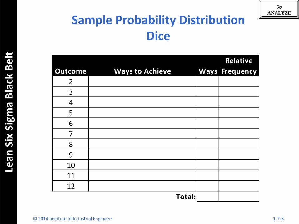
Dice Distribution

• Create a theoretical distribution for a pair of dice.

• How many of each outcome would you expect if you rolled the dice 100 times?


6s

ANALYZE Le

an S

ix S

igm

a B

lack

Be

lt

Sample Probability Distribution Dice

Outcome Ways to Achieve Ways

Relative

Frequency

2

3

4

5

6

7

8

9

10

11

12

Total:


6s

ANALYZE Le

an S

ix S

igm

a B

lack

Be

lt

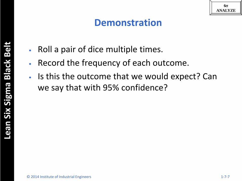
Demonstration

• Roll a pair of dice multiple times.

• Record the frequency of each outcome.

• Is this the outcome that we would expect? Can we say that with 95% confidence?


6s

ANALYZE Le

an S

ix S

igm

a B

lack

Be

lt

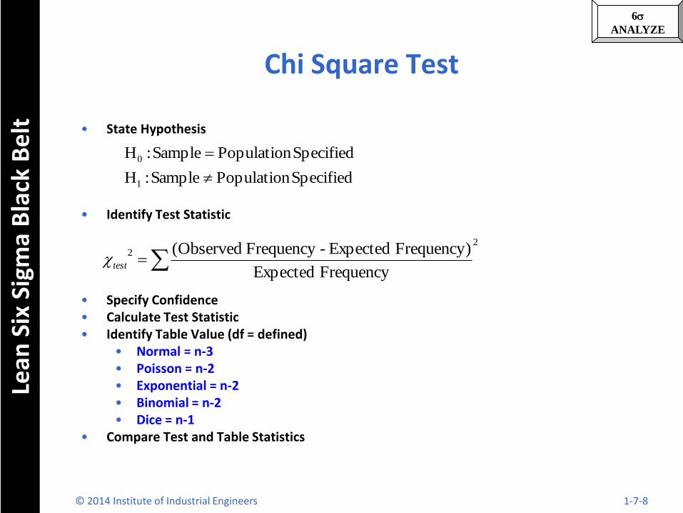
Chi Square Test

• State Hypothesis

• Identify Test Statistic

• Specify Confidence • Calculate Test Statistic • Identify Table Value (df = defined)

• Normal = n-3 • Poisson = n-2 • Exponential = n-2 • Binomial = n-2 • Dice = n-1

• Compare Test and Table Statistics

22

FrequencyExpected

) Frequency Expected- FrequencyObserved(test

Specified Population Sample :H

Specified Population Sample :H

1

0


6s

ANALYZE Le

an S

ix S

igm

a B

lack

Be

lt

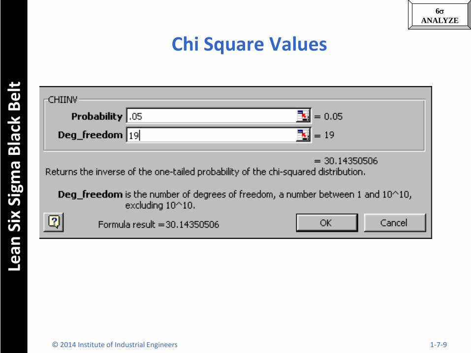
Chi Square Values


6s

ANALYZE Le

an S

ix S

igm

a B

lack

Be

lt

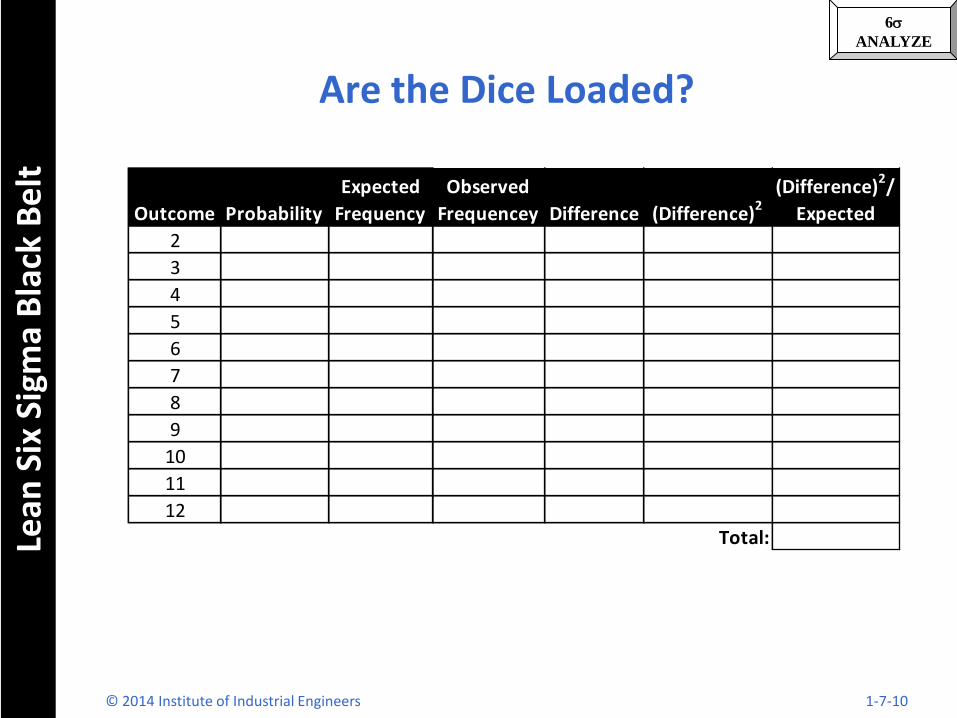
Are the Dice Loaded?

Outcome Probability

Expected

Frequency

Observed

Frequencey Difference (Difference)2(Difference)2/

Expected

2

3

4

5

6

7

8

9

10

11

12

Total:


6s

ANALYZE Le

an S

ix S

igm

a B

lack

Be

lt

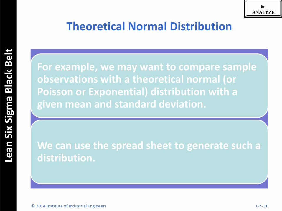
Theoretical Normal Distribution

For example, we may want to compare sample observations with a theoretical normal (or Poisson or Exponential) distribution with a given mean and standard deviation.

We can use the spread sheet to generate such a distribution.


6s

ANALYZE Le

an S

ix S

igm

a B

lack

Be

lt

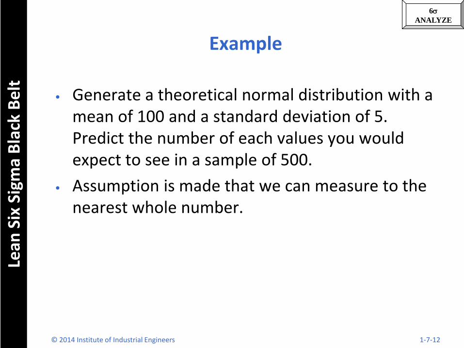
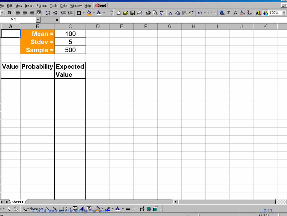
Example

• Generate a theoretical normal distribution with a mean of 100 and a standard deviation of 5. Predict the number of each values you would expect to see in a sample of 500.

• Assumption is made that we can measure to the nearest whole number.


6s

ANALYZE Le

an S

ix S

igm

a B

lack

Be

lt


6s

ANALYZE Le

an S

ix S

igm

a B

lack

Be

lt

Example Continued

Programming the theoretical normal distribution


6s

ANALYZE Le

an S

ix S

igm

a B

lack

Be

lt

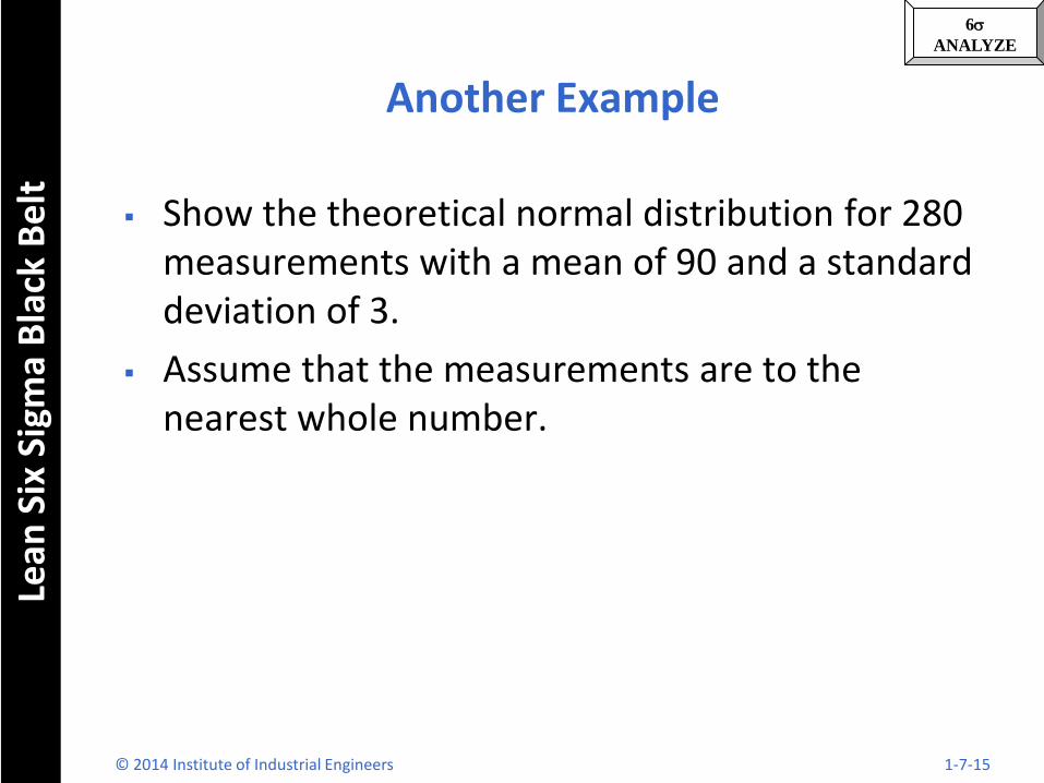
Another Example

Show the theoretical normal distribution for 280 measurements with a mean of 90 and a standard deviation of 3.

Assume that the measurements are to the nearest whole number.


6s

ANALYZE Le

an S

ix S

igm

a B

lack

Be

lt

Example

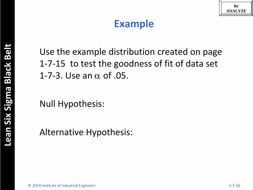
Use the example distribution created on page 1-7-15 to test the goodness of fit of data set 1-7-3. Use an a of .05.

Null Hypothesis:

Alternative Hypothesis:


6s

ANALYZE Le

an S

ix S

igm

a B

lack

Be

lt

Example

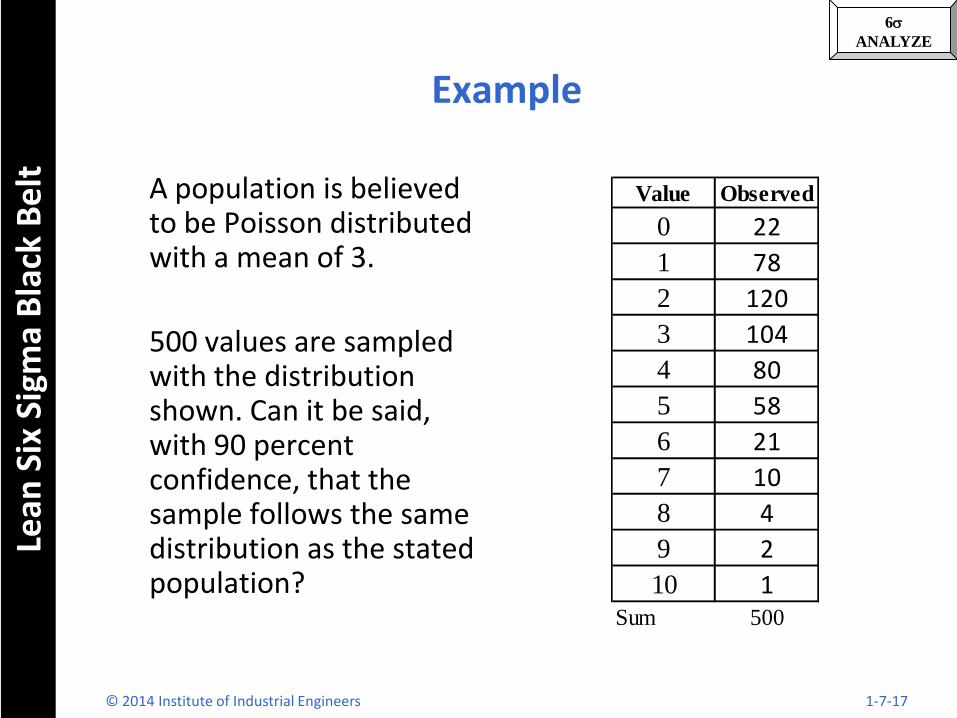
A population is believed to be Poisson distributed with a mean of 3.

500 values are sampled with the distribution shown. Can it be said, with 90 percent confidence, that the sample follows the same distribution as the stated population?

Value Observed

0 22

1 78

2 120

3 104

4 80

5 58

6 21

7 10

8 4

9 2

10 1Sum 500


6s

ANALYZE Le

an S

ix S

igm

a B

lack

Be

lt

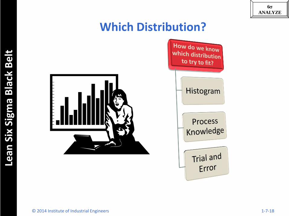
Which Distribution?


6s

ANALYZE Le

an S

ix S

igm

a B

lack

Be

lt

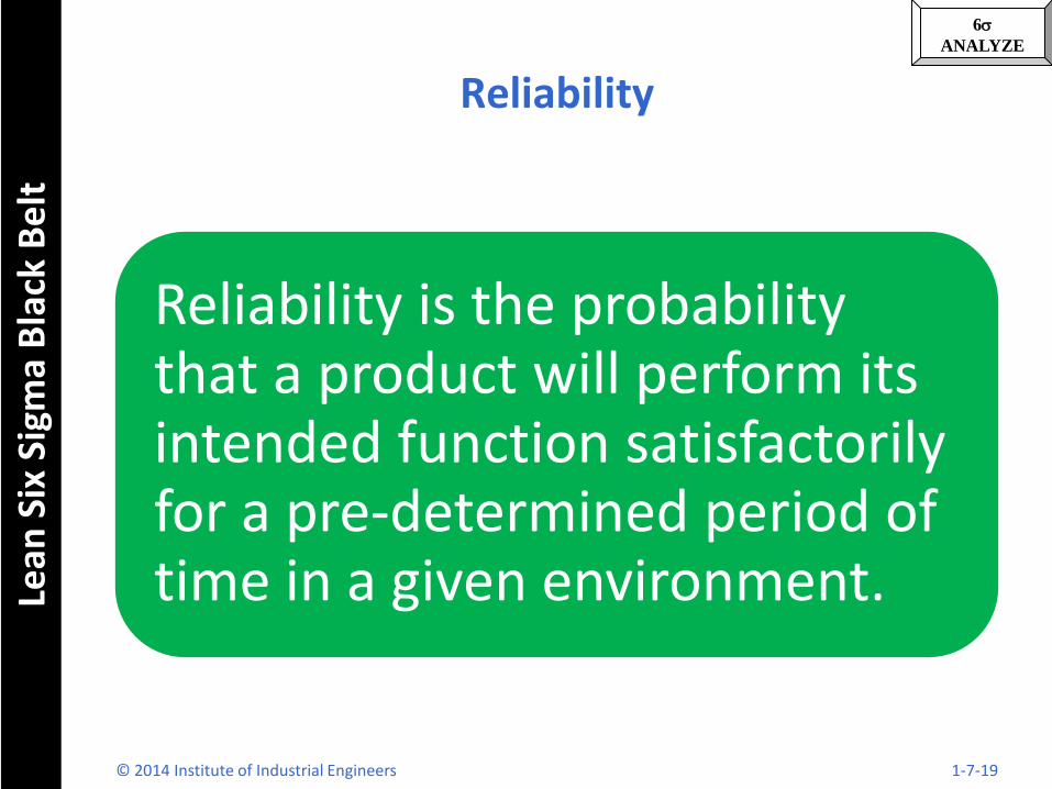
Reliability

Reliability is the probability that a product will perform its intended function satisfactorily for a pre-determined period of time in a given environment.


6s

ANALYZE Le

an S

ix S

igm

a B

lack

Be

lt

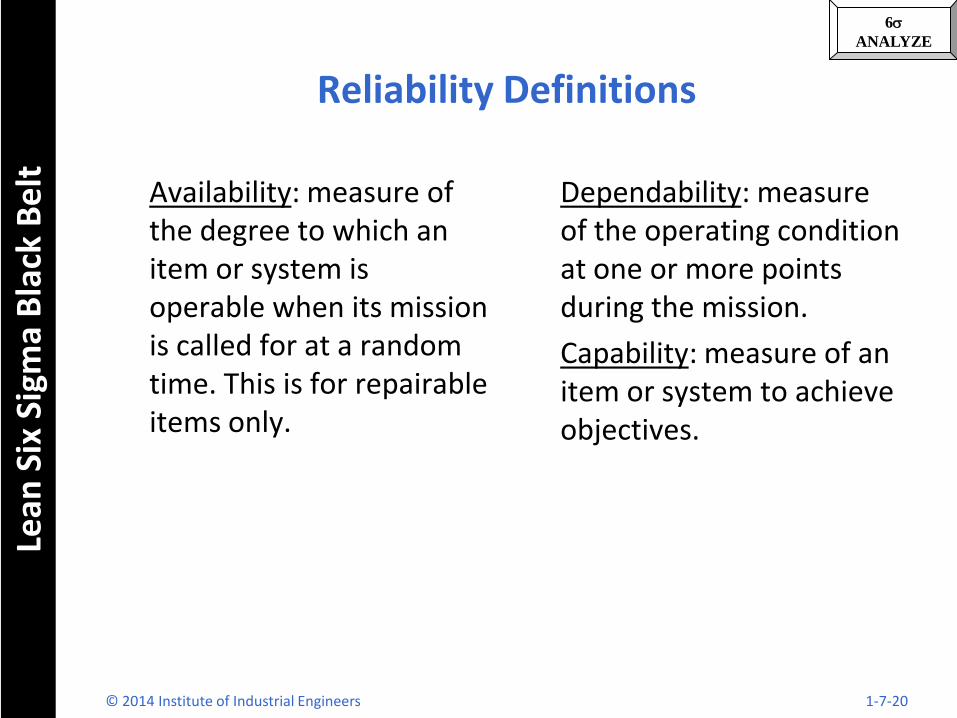
Reliability Definitions

Availability: measure of the degree to which an item or system is operable when its mission is called for at a random time. This is for repairable items only.

Dependability: measure of the operating condition at one or more points during the mission.

Capability: measure of an item or system to achieve objectives.


6s

ANALYZE Le

an S

ix S

igm

a B

lack

Be

lt

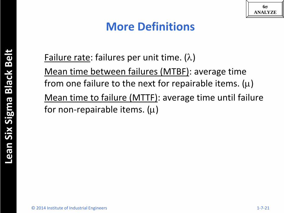
More Definitions

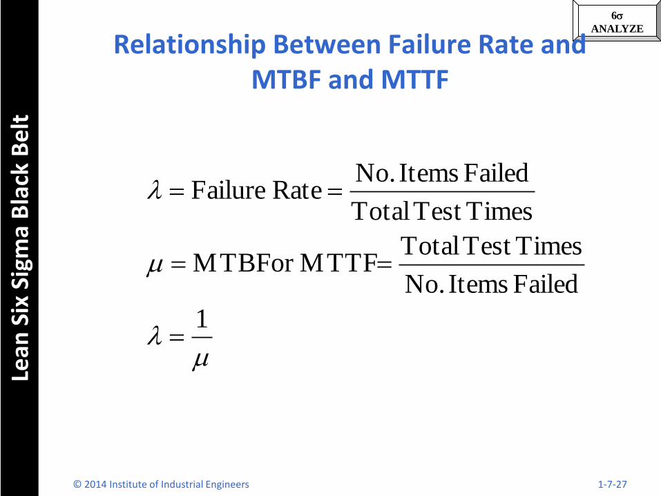
Failure rate: failures per unit time. (l)

Mean time between failures (MTBF): average time from one failure to the next for repairable items. (m)

Mean time to failure (MTTF): average time until failure for non-repairable items. (m)


6s

ANALYZE Le

an S

ix S

igm

a B

lack

Be

lt

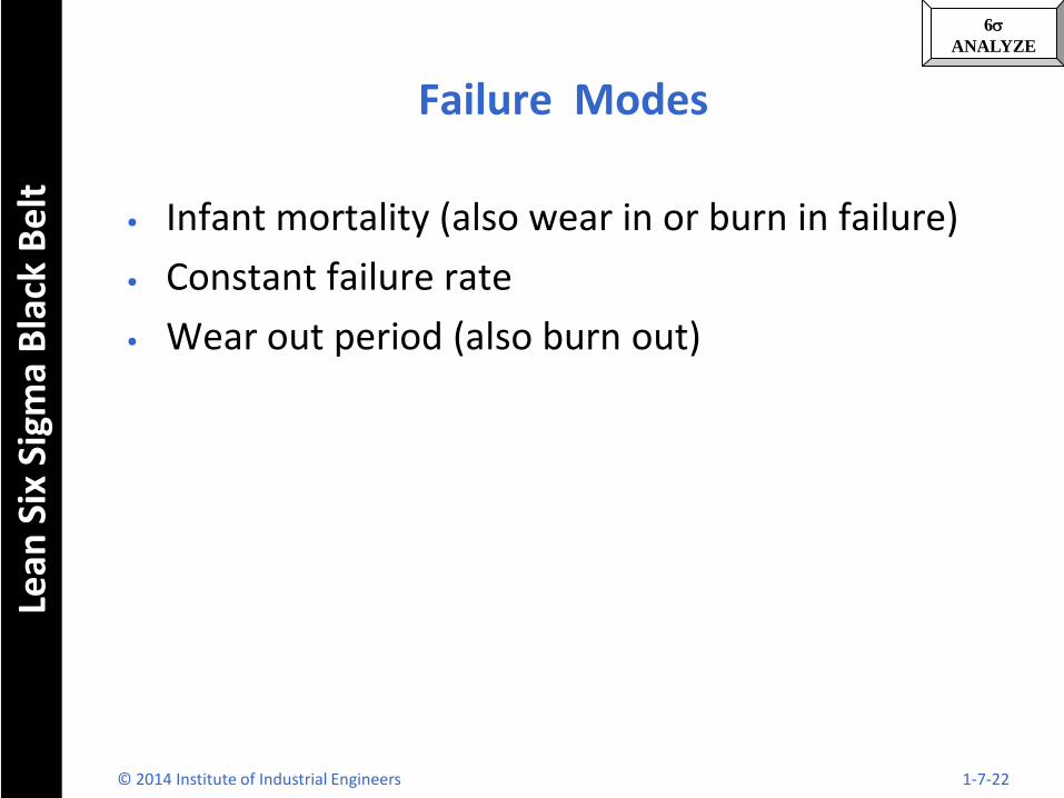
Failure Modes

• Infant mortality (also wear in or burn in failure)

• Constant failure rate

• Wear out period (also burn out)


6s

ANALYZE Le

an S

ix S

igm

a B

lack

Be

lt

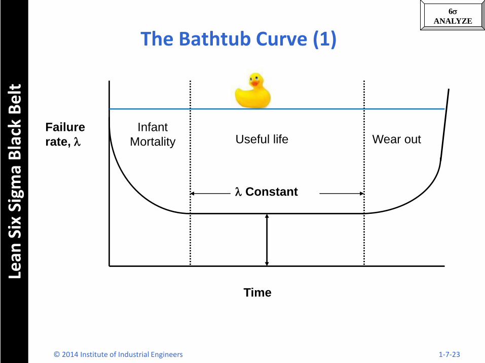
The Bathtub Curve (1)

Time

Failure

rate, l

l Constant

Useful life Wear out Infant

Mortality


6s

ANALYZE Le

an S

ix S

igm

a B

lack

Be

lt

The Bathtub Curve (2)

1. An “infant mortality” early life phase characterized by a decreasing failure rate (Phase 1). Failure occurrence during this period is not random in time but rather the result of substandard components with gross defects and the lack of adequate controls in the manufacturing process. Parts fail at a high but decreasing rate. 2. A “useful life” period where electronics have a relatively constant failure rate caused by randomly occurring defects and stresses (Phase 2). This corresponds to a normal wear and tear period where failures are caused by unexpected and sudden over stress conditions. Most reliability analyses pertaining to electronic systems are concerned with lowering the failure frequency (i.e., lconst shown in the Figure) during this period. 3. A “wear out” period where the failure rate increases due to critical parts wearing out (Phase 3). As they wear out, it takes less stress to cause failure and the overall system failure rate increases, accordingly failures do not occur randomly in time.


6s

ANALYZE Le

an S

ix S

igm

a B

lack

Be

lt

Distribution of Time Between Failures

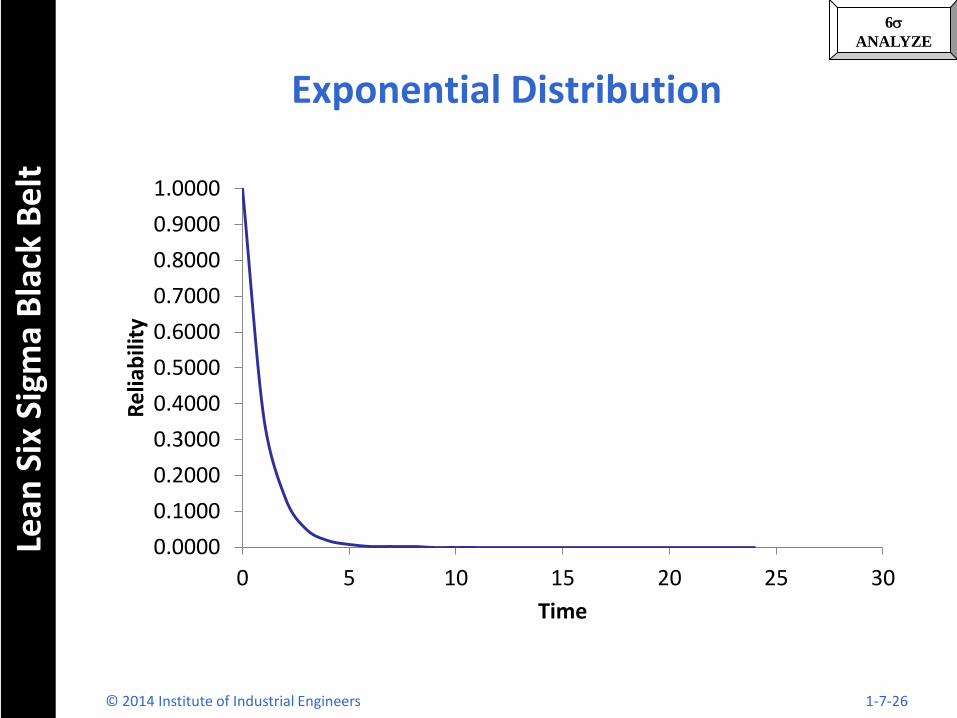
• Along with concern for high failures during the infant mortality period, customers must be concerned with the length of time that a product will run without failure.

• Often this failure rate is constant with the time between failures distributed exponentially.


6s

ANALYZE Le

an S

ix S

igm

a B

lack

Be

lt

Exponential Distribution

0.0000

0.1000

0.2000

0.3000

0.4000

0.5000

0.6000

0.7000

0.8000

0.9000

1.0000

0 5 10 15 20 25 30

Re

liab

ility

Time


6s

ANALYZE Le

an S

ix S

igm

a B

lack

Be

lt

Relationship Between Failure Rate and MTBF and MTTF

ml

m

l

1

Failed Items No.

TimesTest Total MTTFor MTBF

TimesTest Total

Failed Items No.Rate Failure


6s

ANALYZE Le

an S

ix S

igm

a B

lack

Be

lt

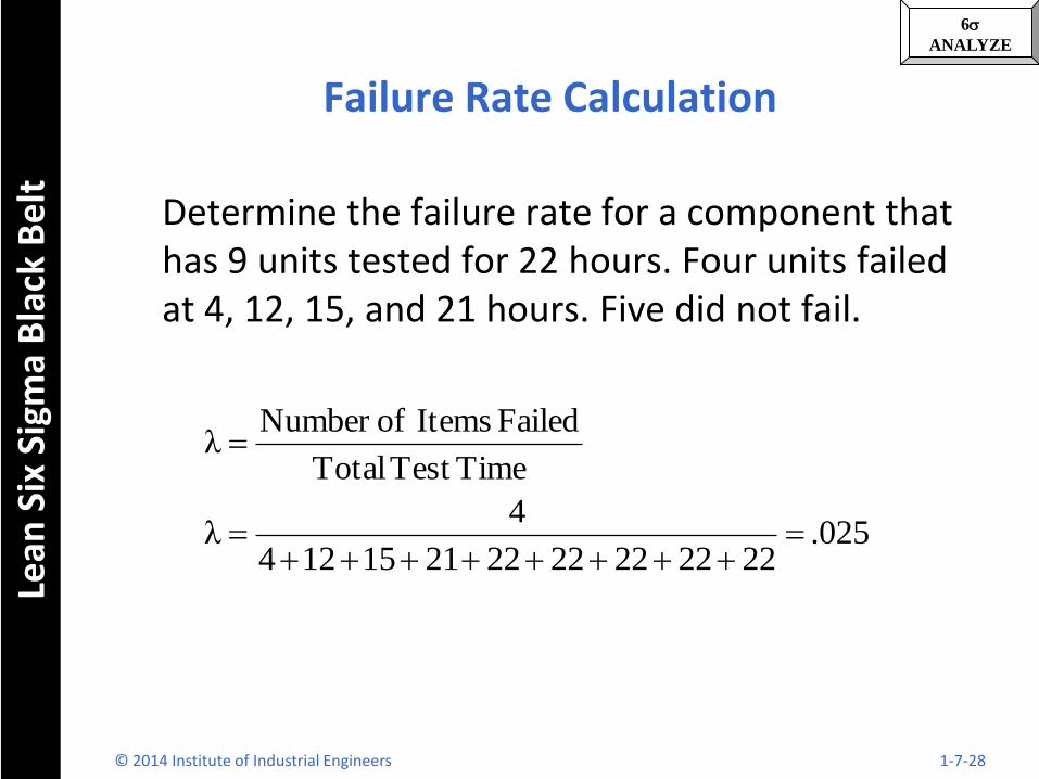
Failure Rate Calculation

Determine the failure rate for a component that has 9 units tested for 22 hours. Four units failed at 4, 12, 15, and 21 hours. Five did not fail.

025.22222222222115124

4λ

TimeTest Total

Failed Items ofNumber λ


6s

ANALYZE Le

an S

ix S

igm

a B

lack

Be

lt

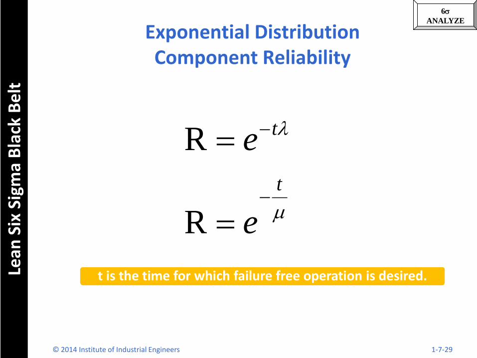
Exponential Distribution Component Reliability

m

l

t

t

e

e

R

R

t is the time for which failure free operation is desired.


6s

ANALYZE Le

an S

ix S

igm

a B

lack

Be

lt

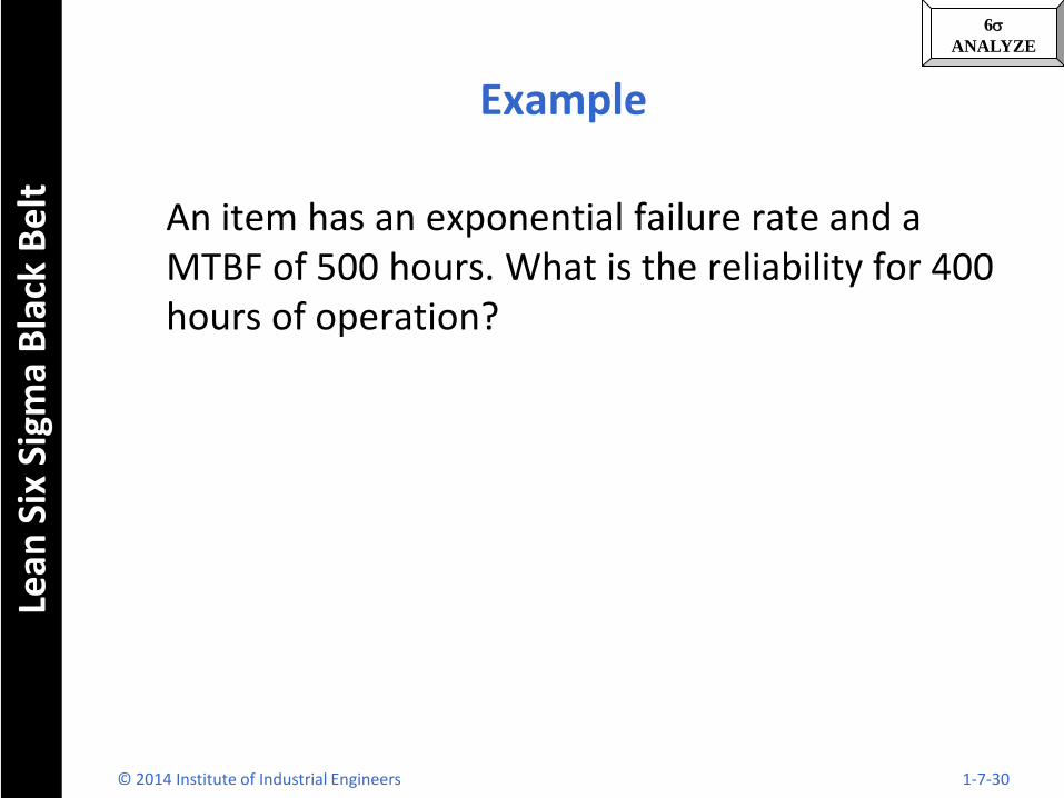
Example

An item has an exponential failure rate and a MTBF of 500 hours. What is the reliability for 400 hours of operation?


6s

ANALYZE Le

an S

ix S

igm

a B

lack

Be

lt

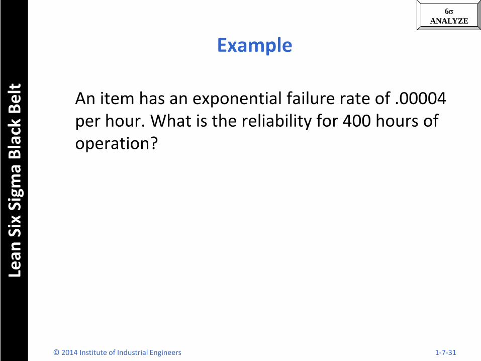
Example

An item has an exponential failure rate of .00004 per hour. What is the reliability for 400 hours of operation?


6s

ANALYZE Le

an S

ix S

igm

a B

lack

Be

lt

System Reliability

Series Design

Parallel Design


6s

ANALYZE Le

an S

ix S

igm

a B

lack

Be

lt

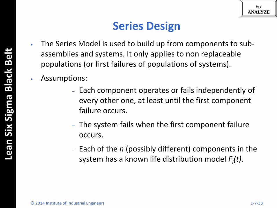
Series Design

• The Series Model is used to build up from components to sub-assemblies and systems. It only applies to non replaceable populations (or first failures of populations of systems).

• Assumptions:

– Each component operates or fails independently of every other one, at least until the first component failure occurs.

– The system fails when the first component failure occurs.

– Each of the n (possibly different) components in the system has a known life distribution model Fi(t).


6s

ANALYZE Le

an S

ix S

igm

a B

lack

Be

lt

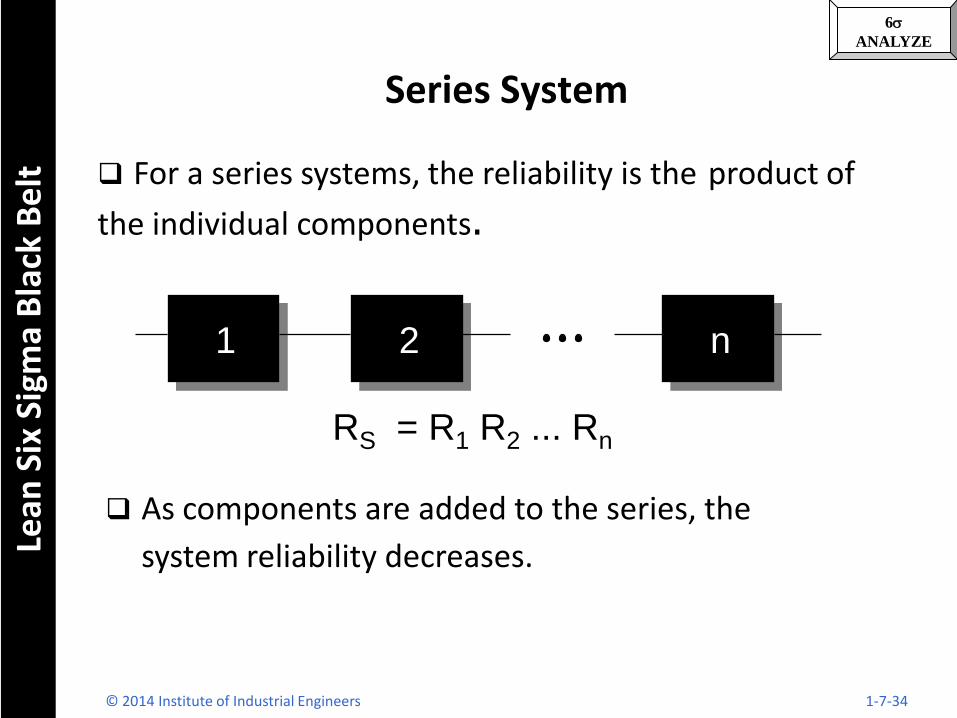
RS = R1 R2 ... Rn

1 2 n

For a series systems, the reliability is the product of

the individual components.

As components are added to the series, the

system reliability decreases.

Series System


6s

ANALYZE Le

an S

ix S

igm

a B

lack

Be

lt

Series Reliability

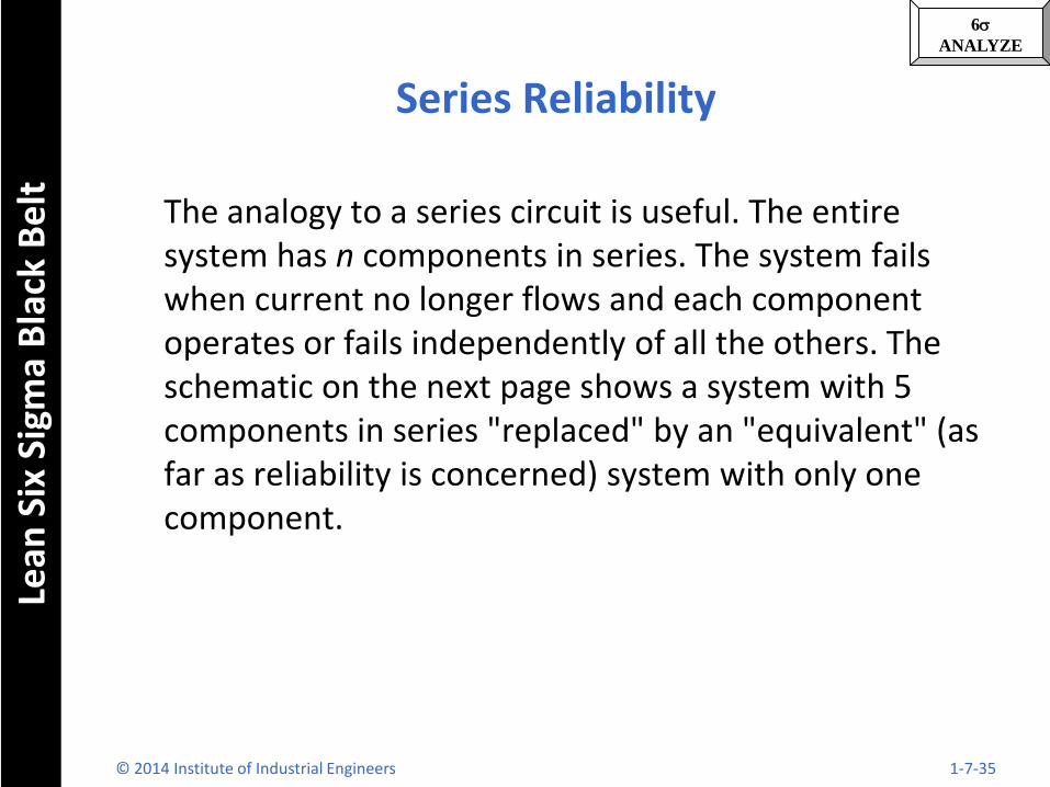
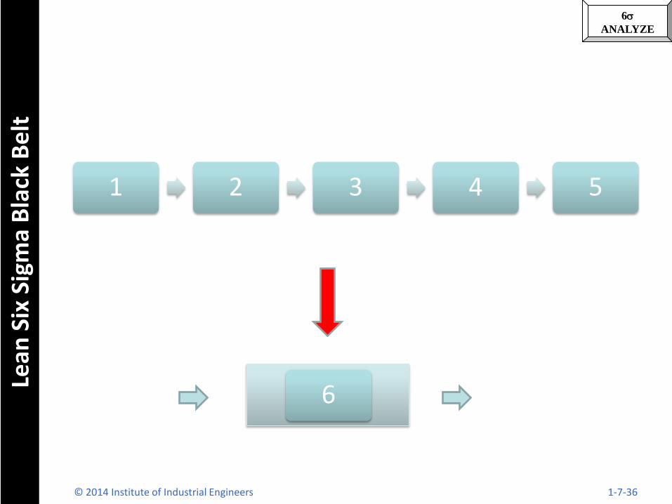
The analogy to a series circuit is useful. The entire system has n components in series. The system fails when current no longer flows and each component operates or fails independently of all the others. The schematic on the next page shows a system with 5 components in series "replaced" by an "equivalent" (as far as reliability is concerned) system with only one component.


6s

ANALYZE Le

an S

ix S

igm

a B

lack

Be

lt

1 2 3 4 5

6


6s

ANALYZE Le

an S

ix S

igm

a B

lack

Be

lt

Example

If in the preceding diagram each component had a reliability of .85 what would the system reliability be?


6s

ANALYZE Le

an S

ix S

igm

a B

lack

Be

lt

Parallel Reliability

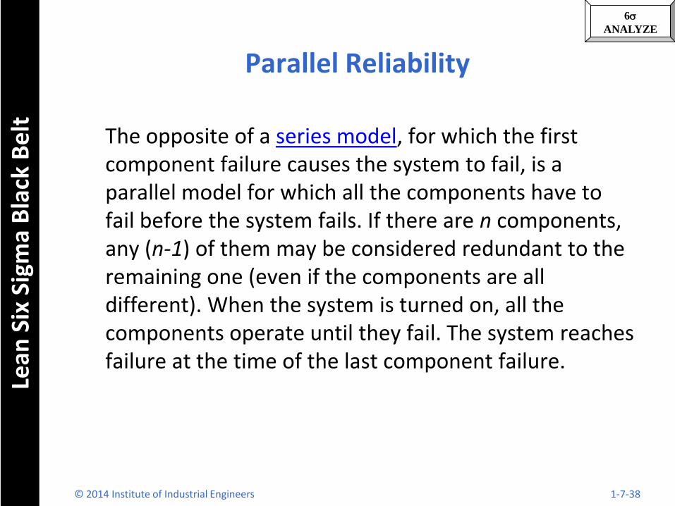
The opposite of a series model, for which the first component failure causes the system to fail, is a parallel model for which all the components have to fail before the system fails. If there are n components, any (n-1) of them may be considered redundant to the remaining one (even if the components are all different). When the system is turned on, all the components operate until they fail. The system reaches failure at the time of the last component failure.


6s

ANALYZE Le

an S

ix S

igm

a B

lack

Be

lt

Parallel

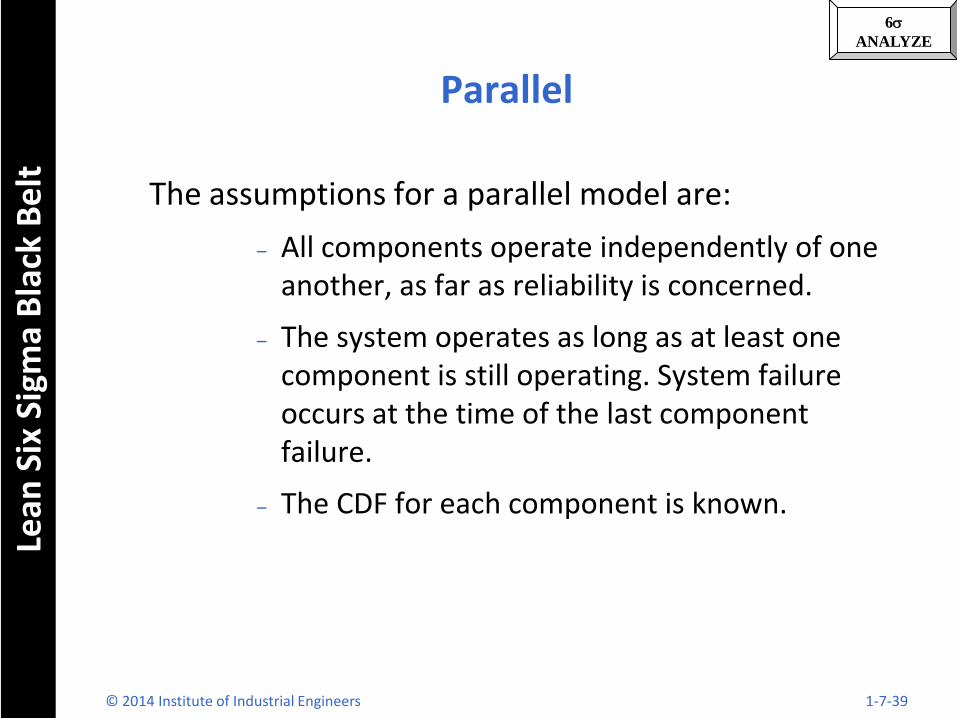
The assumptions for a parallel model are:

– All components operate independently of one another, as far as reliability is concerned.

– The system operates as long as at least one component is still operating. System failure occurs at the time of the last component failure.

– The CDF for each component is known.


6s

ANALYZE Le

an S

ix S

igm

a B

lack

Be

lt

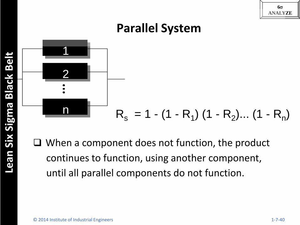
Rs = 1 - (1 - R1) (1 - R2)... (1 - Rn)

1

2

n

When a component does not function, the product

continues to function, using another component,

until all parallel components do not function.

Parallel System


6s

ANALYZE Le

an S

ix S

igm

a B

lack

Be

lt

Parallel Model

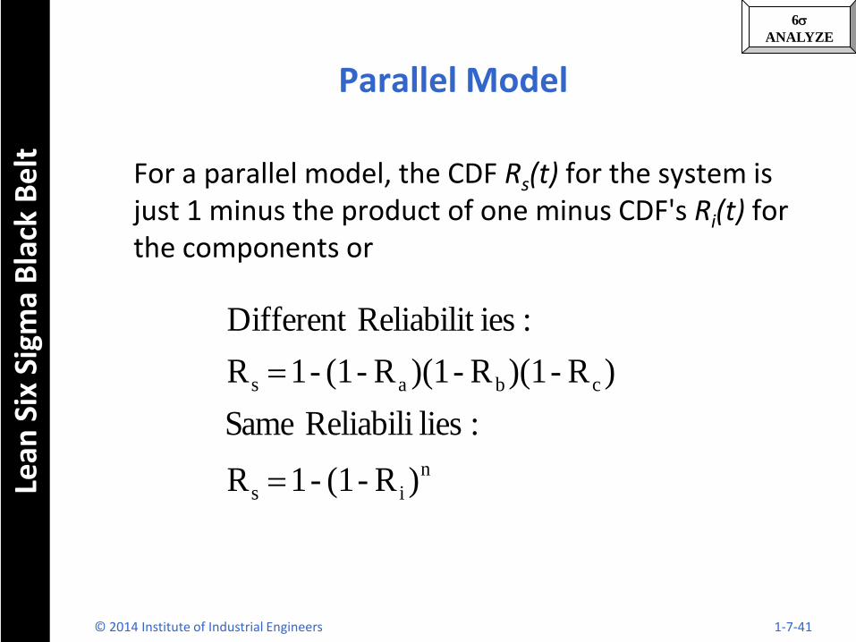
For a parallel model, the CDF Rs(t) for the system is just 1 minus the product of one minus CDF's Ri(t) for the components or

n

is

cbas

)R-(1 - 1 R

:lies ReliabiliSame

)R-)(1R-)(1R-(1-1 R

:iesReliabilitDifferent


6s

ANALYZE Le

an S

ix S

igm

a B

lack

Be

lt

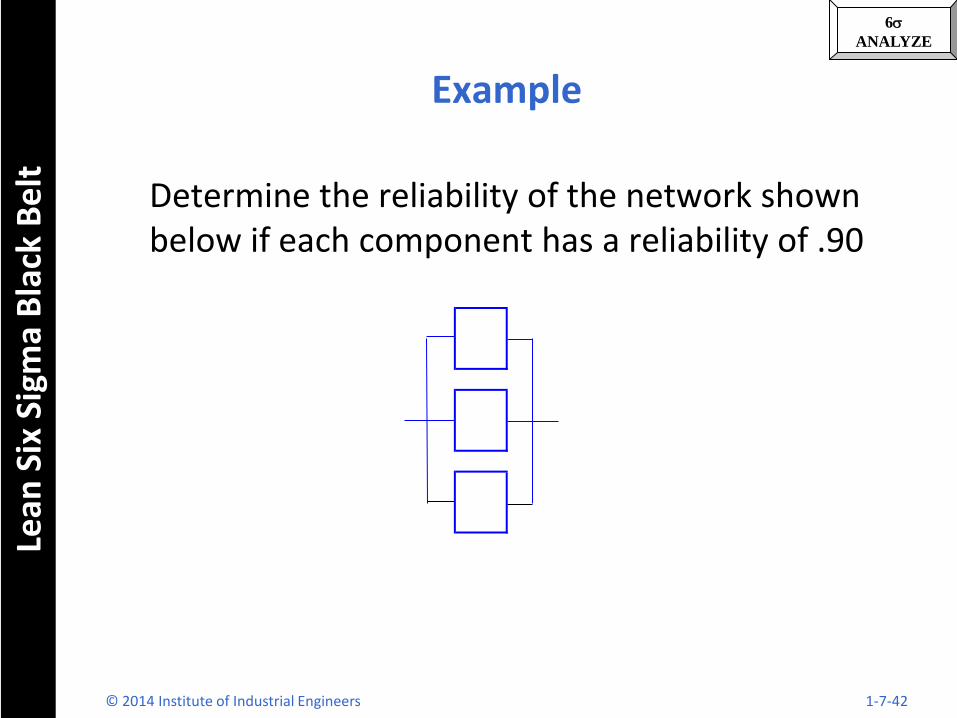
Example

Determine the reliability of the network shown below if each component has a reliability of .90


6s

ANALYZE Le

an S

ix S

igm

a B

lack

Be

lt

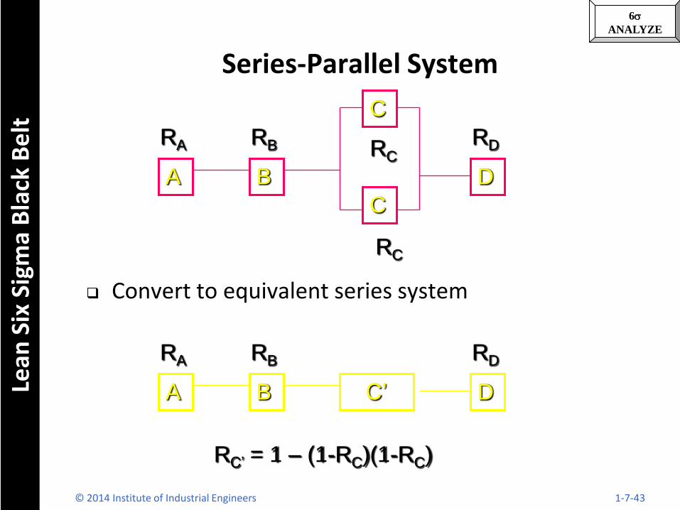
Convert to equivalent series system

A B

C

C

D

RA RB RC

RD

RC

A B C’ D

RA RB RD

RC’ = 1 – (1-RC)(1-RC)

Series-Parallel System


6s

ANALYZE Le

an S

ix S

igm

a B

lack

Be

lt

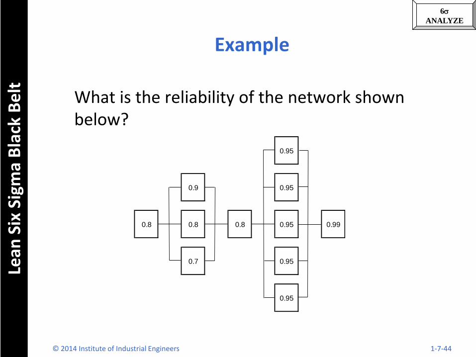
Example

What is the reliability of the network shown below?

0.95

0.9 0.95

0.8 0.8 0.8 0.95 0.99

0.7 0.95

0.95


6s

ANALYZE Le

an S

ix S

igm

a B

lack

Be

lt

Reference

http://www.itl.nist.gov/div898/handbook/


Documents

Chapter 1-7 Goodness of Fit Testing Reliability · 6s ANALYZE Belt Expected Value The expected value is the probability of an event times the sample size. The probability of finding