Chapter 1 · Chapter 1 A PRIMER IN COLUMN ... linear and in particular in integer programming. We touch on both, ... BB0: The linear programming relaxation of the master problem

Chapter 1

A PRIMER IN COLUMN GENERATION

Jacques DesrosiersMarco E. Lubbecke

Abstract We give a didactic introduction to the use of the column generation technique inlinear and in particular in integer programming. We touch on both, the relevantbasic theory and more advanced ideas which help in solving large scale practicalproblems. Our discussion includes embedding Dantzig-Wolfe decomposition andLagrangian relaxation within a branch-and-bound framework, deriving naturalbranching and cutting rules by means of a so-called compact formulation, andunderstanding and influencing the behavior of the dual variables during columngeneration. Most concepts are illustrated via a small example. We close with adiscussion of the classical cutting stock problem and some suggestions for furtherreading.

1. Hands-On ExperienceLet us start right away by solving a constrained shortest path problem. Con-

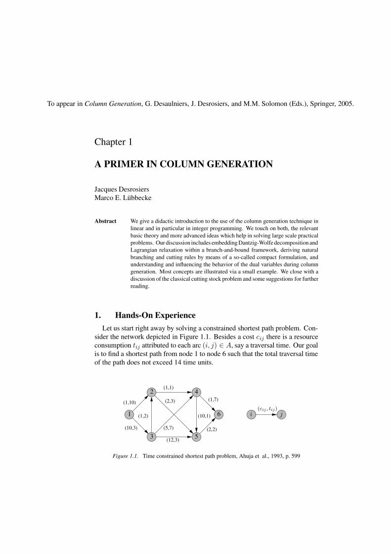
sider the network depicted in Figure 1.1. Besides a cost cij there is a resourceconsumption tij attributed to each arc (i, j) ∈ A, say a traversal time. Our goalis to find a shortest path from node 1 to node 6 such that the total traversal timeof the path does not exceed 14 time units.

To appear in Column Generation, G. Desaulniers, J. Desrosiers, and M.M. Solomon (Eds.), Springer, 2005.

3 5

1

42

i6 j(cij , tij)

(2,3)

(5,7)

(10,1)

(2,2)

(12,3)

(1,7)

(1,1)

(1,2)

(1,10)

(10,3)

Figure 1.1. Time constrained shortest path problem, Ahuja et al., 1993, p. 599

2

One way to state this particular network flow problem is as the integer pro-gram (1.1)–(1.6). One unit of flow has to leave the source (1.2) and has to enterthe sink (1.4), while flow conservation (1.3) holds at all other nodes. The timeresource constraint appears as (1.5).

z? := min∑

(i,j)∈A

cijxij (1.1)

subject to∑

j:(1,j)∈A

x1j = 1 (1.2)

∑

j:(i,j)∈A

xij −∑

j:(j,i)∈A

xji = 0 i = 2, 3, 4, 5 (1.3)

∑

i:(i,6)∈A

xi6 = 1 (1.4)

∑

(i,j)∈A

tijxij ≤ 14 (1.5)

xij = 0 or 1 (i, j) ∈ A (1.6)

An inspection shows that there are nine possible paths, three of which consumetoo much time. The optimal integer solution is path 13246 of cost 13 with atraversal time of 13. How would we find this out? First note that the resourceconstraint (1.5) prevents us from solving our problem with a classical shortestpath algorithm. In fact, no polynomial time algorithm is likely to exist sincethe resource constrained shortest path problem is NP-hard. However, sincethe problem is almost a shortest path problem, we would like to exploit thisembedded well-studied structure algorithmically.

1.1 An Equivalent Reformulation: Arcs vs. PathsIf we ignore the complicating constraint (1.5), the easily tractable remainder

is X = {xij = 0 or 1 | (1.2)–(1.4)}. It is a well-known result in networkflow theory that an extreme point xp = (xpij) of the polytope defined by theconvex hull of X corresponds to a path p ∈ P in the network. This enables usto express any arc flow as a convex combination of path flows:

xij =∑

p∈P

xpijλp (i, j) ∈ A (1.7)

∑

p∈P

λp = 1 (1.8)

λp ≥ 0 p ∈ P. (1.9)

A Primer in Column Generation 3

If we substitute for x in (1.1) and (1.5) we obtain the so-called master problem:

z? = min∑

p∈P

(∑

(i,j)∈A

cijxpij)λp (1.10)

subject to∑

p∈P

(∑

(i,j)∈A

tijxpij)λp ≤ 14 (1.11)

∑

p∈P

λp = 1 (1.12)

λp ≥ 0 p ∈ P (1.13)∑

p∈P

xpijλp = xij (i, j) ∈ A (1.14)

xij = 0 or 1 (i, j) ∈ A . (1.15)

Loosely speaking, the structural information X that we are looking for a pathis hidden in “p ∈ P .” The cost coefficient of λp is the cost of path p and itscoefficient in (1.11) is path p’s duration. Via (1.14) and (1.15) we explicitlypreserve the linking of variables (1.7) in the formulation, and we may recover asolution x to our original problem (1.1)–(1.6) from a master problem’s solution.Always remember that integrality must hold for the original x variables.

1.2 The Linear Relaxation of the Master ProblemOne starts with solving the linear programming (LP) relaxation of the master

problem. If we relax (1.15), there is no longer a need to link the x and λ

variables, and we may drop (1.14) as well. There remains a problem withnine path variables and two constraints. Associate with (1.11) and (1.12) dualvariables π1 and π0, respectively. For large networks, the cardinality of Pbecomes prohibitive, and we cannot even explicitly state all the variables of themaster problem. The appealing idea of column generation is to work only witha sufficiently meaningful subset of variables, forming the so-called restrictedmaster problem (RMP). More variables are added only when needed: like inthe simplex method we have to find in every iteration a promising variable toenter the basis. In column generation an iteration consists (a) of optimizing therestricted master problem in order to determine the current optimal objectivefunction value z and dual multipliers π, and (b) of finding, if there still is one,a variable λp with negative reduced cost

cp =∑

(i,j)∈A

cijxpij − π1(∑

(i,j)∈A

tijxpij) − π0 < 0. (1.16)

The implicit search for a minimum reduced cost variable amounts to optimizinga subproblem, precisely in our case: a shortest path problem in the network of

4

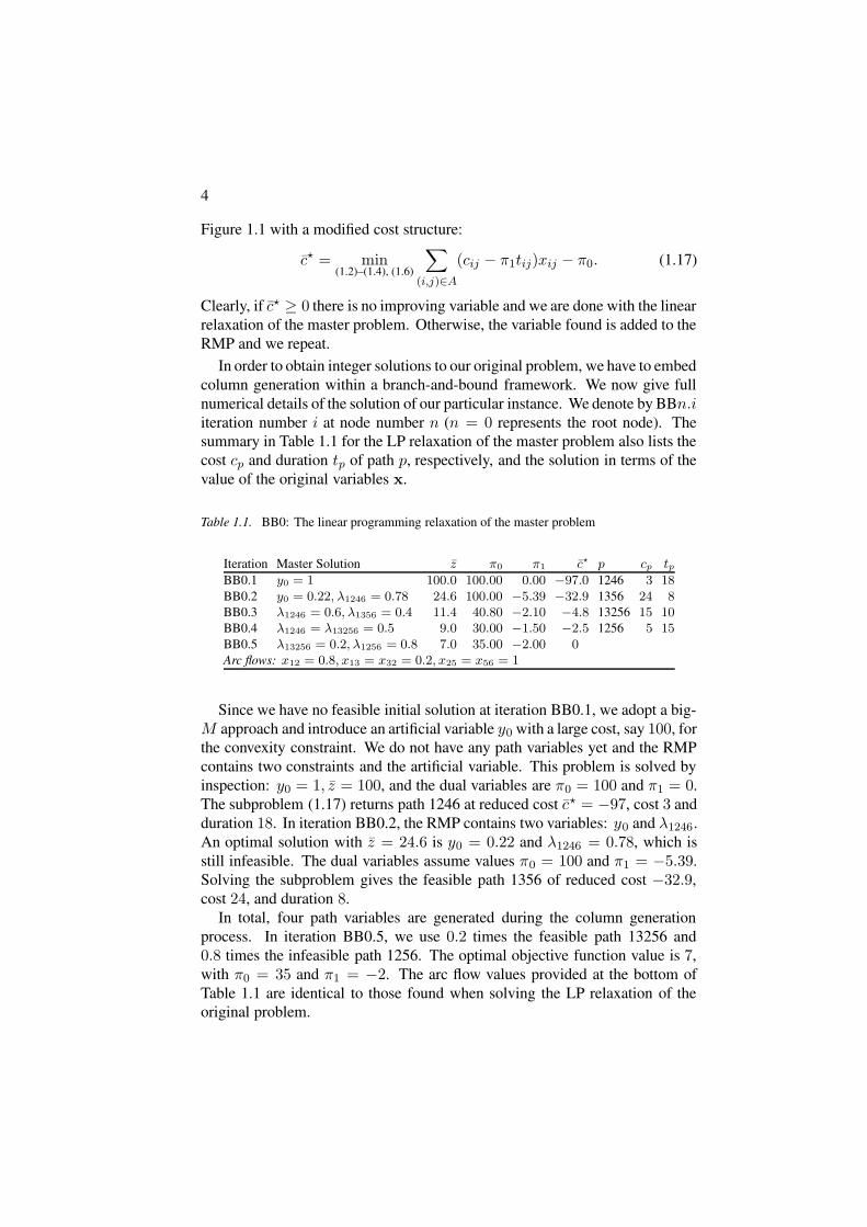
Figure 1.1 with a modified cost structure:

c? = min(1.2)–(1.4), (1.6)

∑

(i,j)∈A

(cij − π1tij)xij − π0. (1.17)

Clearly, if c? ≥ 0 there is no improving variable and we are done with the linearrelaxation of the master problem. Otherwise, the variable found is added to theRMP and we repeat.

In order to obtain integer solutions to our original problem, we have to embedcolumn generation within a branch-and-bound framework. We now give fullnumerical details of the solution of our particular instance. We denote by BBn.iiteration number i at node number n (n = 0 represents the root node). Thesummary in Table 1.1 for the LP relaxation of the master problem also lists thecost cp and duration tp of path p, respectively, and the solution in terms of thevalue of the original variables x.

Table 1.1. BB0: The linear programming relaxation of the master problem

Iteration Master Solution z π0 π1 c? p cp tp

BB0.1 y0 = 1 100.0 100.00 0.00 −97.0 1246 3 18BB0.2 y0 = 0.22, λ1246 = 0.78 24.6 100.00 −5.39 −32.9 1356 24 8BB0.3 λ1246 = 0.6, λ1356 = 0.4 11.4 40.80 −2.10 −4.8 13256 15 10BB0.4 λ1246 = λ13256 = 0.5 9.0 30.00 −1.50 −2.5 1256 5 15BB0.5 λ13256 = 0.2, λ1256 = 0.8 7.0 35.00 −2.00 0Arc flows: x12 = 0.8, x13 = x32 = 0.2, x25 = x56 = 1

Since we have no feasible initial solution at iteration BB0.1, we adopt a big-M approach and introduce an artificial variable y0 with a large cost, say 100, forthe convexity constraint. We do not have any path variables yet and the RMPcontains two constraints and the artificial variable. This problem is solved byinspection: y0 = 1, z = 100, and the dual variables are π0 = 100 and π1 = 0.The subproblem (1.17) returns path 1246 at reduced cost c? = −97, cost 3 andduration 18. In iteration BB0.2, the RMP contains two variables: y0 and λ1246.An optimal solution with z = 24.6 is y0 = 0.22 and λ1246 = 0.78, which isstill infeasible. The dual variables assume values π0 = 100 and π1 = −5.39.Solving the subproblem gives the feasible path 1356 of reduced cost −32.9,cost 24, and duration 8.

In total, four path variables are generated during the column generationprocess. In iteration BB0.5, we use 0.2 times the feasible path 13256 and0.8 times the infeasible path 1256. The optimal objective function value is 7,with π0 = 35 and π1 = −2. The arc flow values provided at the bottom ofTable 1.1 are identical to those found when solving the LP relaxation of theoriginal problem.


1.3 Branch-and-Bound: The Reformulation RepeatsExcept for the integrality requirement (1.6) (or 1.15) all constraints of the

original (and of the master) problem are satisfied, and a subsequent branch-and-bound process is used to compute an optimal integer solution. Even though itcannot happen for our example problem, in general the generated set of columnsmay not contain an integer feasible solution. To proceed, we have to start thereformulation and column generation again in each node.

Let us first explore some “standard” ways of branching on fractional vari-ables, e.g., branching on x12 = 0.8. For x12 = 0, the impact on the RMP is thatwe have to remove path variables λ1246 and λ1256, that is, those paths whichcontain arc (1, 2). In the subproblem, this arc is removed from the network.When the RMP is re-optimized, the artificial variable assumes a positive value,and we would have to generate new λ variables. On branch x12 = 1, arcs(1, 3) and (3, 2) cannot be used. Generated paths which contain these arcs arediscarded from the RMP, and both arcs are removed from the subproblem.

There are also many strategies involving more than a single arc flow variable.One is to branch on the sum of all flow variables which currently is 3.2. Sincethe solution is a path, an integer number of arcs has to be used, in fact, atleast three and at most five in our example. Our freedom of making branchingdecisions is a powerful tool when properly applied.

Alternatively, we branch on x13 + x32 = 0.4. On branch x13 + x32 = 0,we simultaneously treat two flow variables; impacts on the RMP and the sub-problem are similar to those described above. On branch x13 + x32 ≥ 1, thisconstraint is first added to the original formulation. We exploit again the pathsubstructure X , go through the reformulation process via (1.7), and obtain anew RMP to work with. Details of the search tree are summarized in Table 1.2.

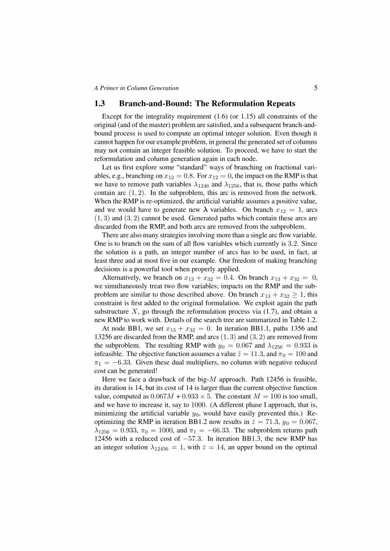
At node BB1, we set x13 + x32 = 0. In iteration BB1.1, paths 1356 and13256 are discarded from the RMP, and arcs (1, 3) and (3, 2) are removed fromthe subproblem. The resulting RMP with y0 = 0.067 and λ1256 = 0.933 isinfeasible. The objective function assumes a value z = 11.3, and π0 = 100 andπ1 = −6.33. Given these dual multipliers, no column with negative reducedcost can be generated!

Here we face a drawback of the big-M approach. Path 12456 is feasible,its duration is 14, but its cost of 14 is larger than the current objective functionvalue, computed as 0.067M + 0.933 × 5. The constant M = 100 is too small,and we have to increase it, say to 1000. (A different phase I approach, that is,minimizing the artificial variable y0, would have easily prevented this.) Re-optimizing the RMP in iteration BB1.2 now results in z = 71.3, y0 = 0.067,λ1256 = 0.933, π0 = 1000, and π1 = −66.33. The subproblem returns path12456 with a reduced cost of −57.3. In iteration BB1.3, the new RMP hasan integer solution λ12456 = 1, with z = 14, an upper bound on the optimal

6

Table 1.2. Details of the branch-and-bound decisions

Iteration Master Solution z π0 π1 π2 c? p cp tp

BB1: BB0 and x13 + x32 = 0BB1.1 y0 = 0.067, λ1256 = 0.933 11.3 100 −6.33 – 0BB1.2 Big-M increased to 1000

y0 = 0.067, λ1256 = 0.933 71.3 1000 −66.33 – −57.3 12456 14 14BB1.3 λ12456 = 1 14 1000 −70.43 – 0

BB2: BB0 and x13 + x32 ≥ 1BB2.1 λ1246 = λ13256 = 0.5 9 15 −0.67 3.33 0Arc flows: x12 = x13 = x24 = x25 = x32 = x46 = x56 = 0.5

BB3: BB2 and x12 = 0BB3.1 λ13256 = 1 15 15 0 0 -2 13246 13 13BB3.2 λ13246 = 1 13 13 0 0 0

BB4: BB2 and x12 = 1BB4.1 y0 = 0.067, λ1256 = 0.933 111.3 100 −6.33 100 0Infeasible arc flows

path cost. The dual multipliers are π0 = 1000 and π1 = −70.43, and no newvariable is generated.

At node BB2, we impose x13+x32 ≥ 1 to the original formulation, and again,we reformulate these x variables in terms of the λ variables. The resulting newconstraint (with dual multiplier π2) in the RMP is

∑

p∈P (xp13 + xp32)λp ≥ 1.

From the value of (xp13 + xp32) we learn how often arcs (1, 3) and (3, 2) areused in path p. The current problem at node BB2.1 is the following:

min 100y0 + 3λ1246 + 24λ1356 + 15λ13256 + 5λ1256

subject to: 18λ1246 + 8λ1356 + 10λ13256 + 15λ1256 ≤ 14 [π1]λ1356 + 2λ13256 ≥ 1 [π2]

y0 + λ1246 + λ1356 + λ13256 + λ1256 = 1 [π0]y0, λ1246, λ1356, λ13256, λ1256 ≥ 0

From solving this linear program we obtain an increase in the objectivefunction z from 7 to 9 with variables λ1246 = λ13256 = 0.5, and dual multipliersπ0 = 15, π1 = −0.67, and π2 = 3.33. The new subproblem is given by

c? = min(1.2)–(1.4), (1.6)

∑

(i,j)∈A

(cij − π1tij)xij − π0 − π2(x13 + x32). (1.18)

For these multipliers no path of negative reduced cost exists. The solution ofthe flow variables is x12 = x13 = x24 = x25 = x32 = x46 = x56 = 0.5.

Next, we arbitrarily choose variable x12 = 0.5 to branch on. Two iterationsare needed when x12 is set to zero. In iteration BB3.1, path variables λ1246


and λ1256 are discarded from the RMP and arc (1, 2) is removed from thesubproblem. The RMP is integer feasible with λ13256 = 1 at cost 15. Dualmultipliers are π0 = 15, π1 = 0, and π2 = 0. Path 13246 of reduced cost−2, cost 13 and duration 13 is generated and used in the next iteration BB3.2.Again the RMP is integer feasible with path variable λ13246 = 1 and a new bestinteger solution at cost 13, with dual multipliers π0 = 15, π1 = 0, and π2 = 0for which no path of negative reduced cost exists.

On the alternative branch x12 = 1 the RMP is optimal after a single iteration.In iteration BB4.1, variable x13 can be set to zero and variables λ1356, λ13256,and λ13246 are discarded from the current RMP. After the introduction of anartificial variable y2 in the second row, the RMP is infeasible since y0 > 0 (ascan be seen also from the large objective function value z = 111.3). Given thedual multipliers, no columns of negative reduced cost can be generated, andthe RMP remains infeasible. The optimal solution (found at node BB3) is path13246 of cost 13 with a duration of 13 as well.

2. Some Theoretical BackgroundIn the previous example we already saw all the necessary building blocks

for a column generation based solution approach to integer programs: (1) anoriginal formulation to solve which acts as the control center to facilitate thedesign of natural branching rules and cutting planes; (2) a master problem todetermine the currently optimal dual multipliers and to provide a lower boundat each node of the branch-and-bound tree; (3) a pricing subproblem whichexplicitly reflects an embedded structure we wish to exploit. In this section wedetail the underlying theory.

2.1 Column GenerationLet us call the following linear program the master problem (MP).

z?MP := min

∑

j∈J

cjλj

subject to∑

j∈J

ajλj ≥ b

λj ≥ 0, j ∈ J.

(1.19)

In each iteration of the simplex method we look for a non-basic variable to priceout and enter the basis. That is, given the non-negative vector π of dual variableswe wish to find a j ∈ J which minimizes cj := cj −π

taj . This explicit pricingis a too costly operation when |J | is huge. Instead, we work with a reasonablysmall subset J ′ ⊆ J of columns—the restricted master problem (RMP)—andevaluate reduced costs only by implicit enumeration. Let λ and π assumeprimal and dual optimal solutions of the current RMP, respectively. When

8

columns aj , j ∈ J , are given as elements of a set A, and the cost coefficient cj

can be computed from aj via a function c then the subproblem

c? := min{

c(a) − πta | a ∈ A

}

(1.20)

performs the pricing. If c? ≥ 0, there is no negative cj , j ∈ J , and the solutionλ to the restricted master problem optimally solves the master problem as well.Otherwise, we add to the RMP the column derived from the optimal subproblemsolution, and repeat with re-optimizing the RMP. The process is initialized withan artificial, a heuristic, or a previous (“warm start”) solution. In what regardsconvergence, note that each a ∈ A is generated at most once since no variablein an optimal RMP has negative reduced cost. When dealing with some finiteset A (as is practically always true), the column generation algorithm is exact.In addition, we can make use of bounds. Let z denote the optimal objectivefunction value to the RMP. When an upper bound κ ≥

∑

j∈J λj holds for theoptimal solution of the master problem, we have not only an upper bound z onz?MP in each iteration, but also a lower bound: we cannot reduce z by more

than κ times the smallest reduced cost c?:

z + κc? ≤ z?MP ≤ z. (1.21)

Thus, we may verify the solution quality at any time. In the optimum of (1.19),c? = 0 for the basic variables, and z = z?

MP .

2.2 Dantzig-Wolfe Decomposition for Integer ProgramsIn many applications we are interested in optimizing over a discrete set X .

For X = {x ∈ Zn+ | Dx ≥ d} 6= ∅ we have the special case of integer linear

programming. Consider the following (original or compact) program:

z? := min ctx

subject to Ax ≥ b

x ∈ X.(1.22)

Replacing X by conv(X) in (1.22) does not change z? which we assume tobe finite. The Minkowski and Weyl theorems (see Schrijver, 1986) enable usto represent each x ∈ X as a convex combination of extreme points {xp}p∈P

plus a non-negative combination of extreme rays {xr}r∈R of conv(X), i.e.,

x =∑

p∈P

xpλp +∑

r∈R

xrλr,∑

p∈P

λp = 1, λ ∈ R|P |+|R|+ (1.23)

where the index sets P and R are finite. Substituting for x in (1.22) and applyingthe linear transformations cj = ctxj and aj = Axj , j ∈ P ∪ R we obtain an


equivalent extensive formulation

z? := min∑

p∈P

cpλp +∑

r∈R

crλr (1.24)

subject to∑

p∈P

apλp +∑

r∈R

arλr ≥ b (1.25)

∑

p∈P

λp = 1 (1.26)

λ ≥ 0 (1.27)∑

p∈P

xpλp +∑

r∈R

xrλr = x (1.28)

x ∈ Zn+. (1.29)

Equation (1.26) is referred to as the convexity constraint. When we relax theintegrality of x, there is no need to link x and λ, and we may also relax (1.28).The columns of this special master problem are defined by the extreme pointsand extreme rays of conv(X). We solve the master by column generation toget its optimal objective function value z?

MP . Given an optimal dual solutionπ and π0 to the current RMP, where variable π0 corresponds to the convex-ity constraint, the subproblem is to determine minj∈P{cj − π

taj − π0} andminj∈R{cj − π

taj}. By our previous linear transformation and since π0 is aconstant, this results in

c? := min{

(ct − πtA)x − π0 | x ∈ X

}

. (1.30)

This subproblem is an integer linear program. When c? ≥ 0, there is no negativereduced cost column, and the algorithm terminates. When c? < 0 and finite, anoptimal solution to (1.30) is an extreme point xp of conv(X), and we add thecolumn [ctxp, (Axp)

t, 1]t to the RMP. When c? = −∞ we identify an extremeray xr of conv(X) as a solution x ∈ X to (ct − π

tA)x = 0, and add thecolumn [ctxr, (Axr)

t, 0]t to the RMP.From (1.21) together with the convexity constraint we obtain in each iteration

z + c? ≤ z?MP ≤ z, (1.31)

where z = πtb + π0 is again the optimal objective function value of the RMP.

Since z?MP ≤ z?, z + c? is also a lower bound on z?. In general, z is not a valid

upper bound on z?, except if the current x variables are integer. The algorithmis exact and finite as long as finiteness is ensured in optimizing the RMP.

The original formulation is the starting point to obtain integer solutions in thex variables. Branching and cutting constraints are added there, the reformula-tion as in Section 1.1.1 is re-applied, and the process continues with an updated

10

master problem. It is important to see that it is our choice as to whether theadditional constraints remain in the master problem (as in the previous section)or go into the subproblem (as we will see later).

Pricing Out the Original x Variables. Assume that in (1.22) we have alinear subproblem X = {x ∈ R

n+ | Dx ≥ d} 6= ∅. Column generation then

essentially solves the linear program

min ctx subject to Ax ≥ b, Dx ≥ d, x ≥ 0.

We obtain an optimal primal solutionx but only the dual multipliers π associatedwith the constraint set Ax ≥ b. However, following an idea of Walker, 1969we can also retrieve the dual variables σ associated with Dx ≥ d: it is thevector obtained from solving the linear subproblem in the last iteration of thecolumn generation process. This full dual information allows for a pricing ofthe original variables, and therefore a possible elimination of some of them.Given an upper bound on the integer optimal objective function value of theoriginal problem, one can eliminate an x variable if its reduced cost is largerthan the optimality gap.

In the general case of a linear integer or even non-linear pricing subproblem,the above procedure does not work. Poggi de Aragao and Uchoa, 2003 suggestto directly use the extensive formulation: if we keep the coupling constraint(1.28) in the master problem, it suffices to impose the constraint x ≥ ε, for asmall ε > 0, at the end of the process. The shadow prices of these constraints arethe reduced costs of the x vector of original variables. Note that there is no needto apply the additional constraints to already positive variables. Computationalexperiments underline the benefits of this procedure.

Block Diagonal Structure. For practical problems Dantzig-Wolfe decom-position can typically exploit a block diagonal structure of D, i.e.,

D =

D1

D2

. . .Dκ

d =

d1

d2

...dκ.

(1.32)

Each Xk = {Dkxk ≥ dk, xk ≥ 0 and integer}, k ∈ K := {1, . . . , κ}, givesrise to a representation as in (1.23). The decomposition yields κ subproblems,each with its own convexity constraint and associated dual variable:

ck? := min{(ckT − πtAk)xk − πk

0 | xk ∈ Xk}, k ∈ K. (1.33)

The superscript k to all entities should be interpreted in the canonical way. Thealgorithm terminates when ck? ≥ 0, for all k ∈ K . Otherwise, extreme points


and rays identified in (1.33) give rise to new columns to be added to the RMP. Bylinear programming duality, z = π

tb+∑κ

k=1 πk0 , and we obtain the following

bounds, see Lasdon, 1970:

z +

κ∑

k=1

ck? ≤ z?MP ≤ z. (1.34)

2.3 Useful Working KnowledgeWhen problems get larger and computationally much more difficult than

our small constrained shortest path problem it is helpful to know more aboutmechanisms, their consequences, and how to exploit them.

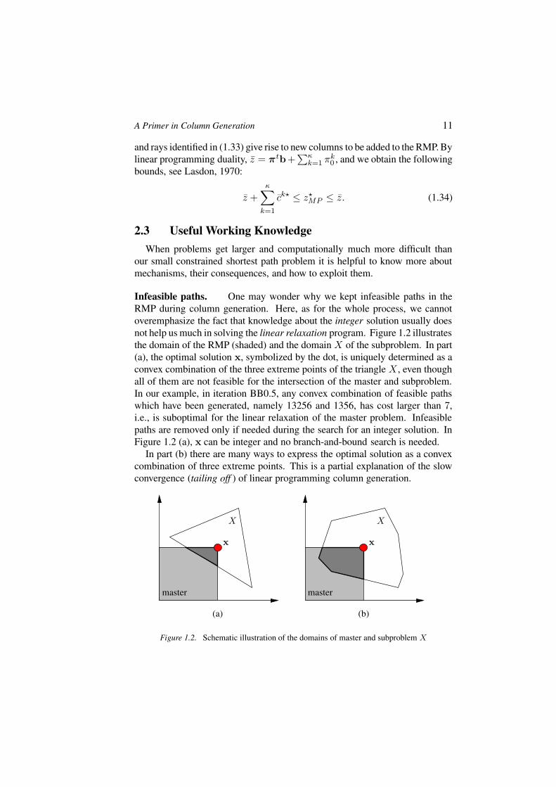
Infeasible paths. One may wonder why we kept infeasible paths in theRMP during column generation. Here, as for the whole process, we cannotoveremphasize the fact that knowledge about the integer solution usually doesnot help us much in solving the linear relaxation program. Figure 1.2 illustratesthe domain of the RMP (shaded) and the domain X of the subproblem. In part(a), the optimal solution x, symbolized by the dot, is uniquely determined as aconvex combination of the three extreme points of the triangle X , even thoughall of them are not feasible for the intersection of the master and subproblem.In our example, in iteration BB0.5, any convex combination of feasible pathswhich have been generated, namely 13256 and 1356, has cost larger than 7,i.e., is suboptimal for the linear relaxation of the master problem. Infeasiblepaths are removed only if needed during the search for an integer solution. InFigure 1.2 (a), x can be integer and no branch-and-bound search is needed.

In part (b) there are many ways to express the optimal solution as a convexcombination of three extreme points. This is a partial explanation of the slowconvergence (tailing off ) of linear programming column generation.

(a)

x x

(b)

XX

master master

Figure 1.2. Schematic illustration of the domains of master and subproblem X

12

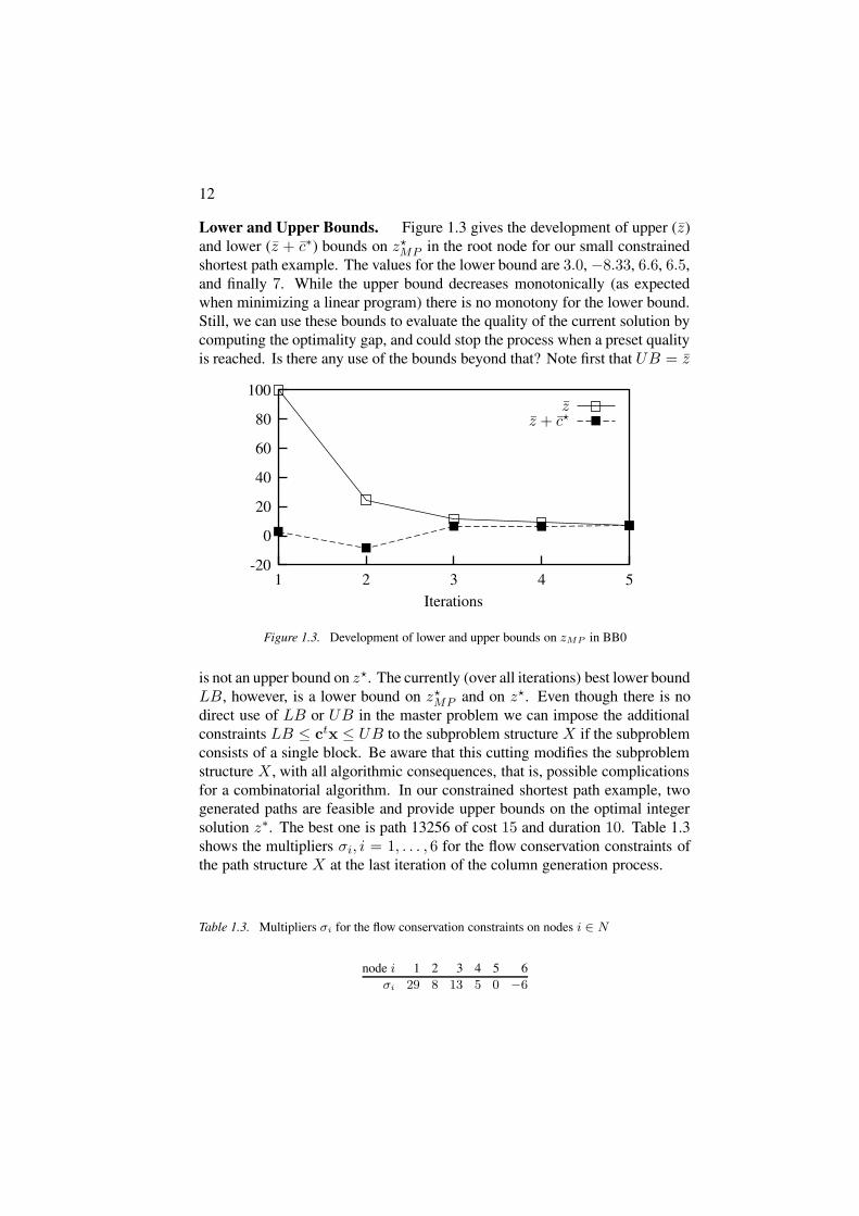
Lower and Upper Bounds. Figure 1.3 gives the development of upper (z)and lower (z + c∗) bounds on z?

MP in the root node for our small constrainedshortest path example. The values for the lower bound are 3.0, −8.33, 6.6, 6.5,and finally 7. While the upper bound decreases monotonically (as expectedwhen minimizing a linear program) there is no monotony for the lower bound.Still, we can use these bounds to evaluate the quality of the current solution bycomputing the optimality gap, and could stop the process when a preset qualityis reached. Is there any use of the bounds beyond that? Note first that UB = z

z + c?z

Iterations54321

100

80

60

40

20

0

-20

Figure 1.3. Development of lower and upper bounds on zMP in BB0

is not an upper bound on z?. The currently (over all iterations) best lower boundLB, however, is a lower bound on z?

MP and on z?. Even though there is nodirect use of LB or UB in the master problem we can impose the additionalconstraints LB ≤ ctx ≤ UB to the subproblem structure X if the subproblemconsists of a single block. Be aware that this cutting modifies the subproblemstructure X , with all algorithmic consequences, that is, possible complicationsfor a combinatorial algorithm. In our constrained shortest path example, twogenerated paths are feasible and provide upper bounds on the optimal integersolution z∗. The best one is path 13256 of cost 15 and duration 10. Table 1.3shows the multipliers σi, i = 1, . . . , 6 for the flow conservation constraints ofthe path structure X at the last iteration of the column generation process.

Table 1.3. Multipliers σi for the flow conservation constraints on nodes i ∈ N

node i 1 2 3 4 5 6σi 29 8 13 5 0 −6


Therefore, given the optimal multiplier π1 = −2 for the resource constraint,the reduced cost of an arc is given by cij = cij − σi + σj − tijπ1, (i, j) ∈ A.The reader can verify that c34 = 3 − 13 + 5 − (7)(−2) = 11. This is theonly reduced cost which exceeds the current optimality gap which equals to15 − 7 = 8. Arc (3, 4) can be permanently discarded from the network andpaths 1346 and 13456 will never be generated.

Integrality Property. Solving the subproblem as an integer program usuallyhelps in closing part of the integrality gap of the master problem (Geoffrion,1974), except when the subproblem possesses the integrality property. Thisproperty means that solutions to the pricing problem are naturally integer whenit is solved as a linear program. This is the case for our shortest path subproblemand this is why we obtained the value of the linear relaxation of the originalproblem as the value of the linear relaxation of the master problem.

When looking for an integer solution to the original problem, we need toimpose new restrictions on (1.1)–(1.6). One way is to take advantage of a newX structure. However, if the new subproblem is still solved as a linear program,z?MP remains 7. Only solving the new X structure as an integer program may

improve z?MP .

Once we understand that we can modify the subproblem structure, we candevise other decomposition strategies. One is to define the X structure as

∑

(i,j)∈A

tijxij ≤ 14, xij binary, (i, j) ∈ A (1.35)

so that the subproblem becomes a knapsack problem which does not possess theintegrality property. Unfortunately, in this example, z?

MP remains 7. However,improvements can be obtained by imposing more and more constraints to thesubproblem. An example is to additionally enforce the selection of one arcto leave the source (1.2) and another one to enter the sink (1.4), and imposeconstraint 3 ≤

∑

(i,j)∈A xij ≤ 5 on the minimum and maximum number ofselected arcs. Richer subproblems, as long as they can be solved efficiently anddo not possess the integrality property, may help in closing the integrality gap.

It is also our decision how much branching and cutting information (rangingfrom none to all) we put into the subproblem. This choice depends on wherethe additional constraints are more easily accommodated in terms of algorithmsand computational tractability. Branching decisions imposed on the subproblemcan reduce its solution space and may turn out to facilitate a solution as integerprogram. As an illustration we describe adding the lower bound cut in the rootnode of our small example.

Imposing the Lower Bound Cut ctx ≥ 7. Assume that we have solvedthe relaxed RMP in the root node and instead of branching, we impose the lower

14

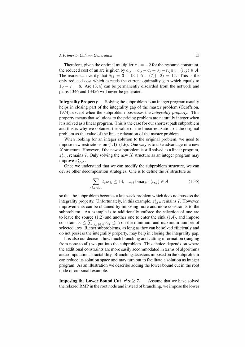
bound cut on the X structure, see Table 1.4. Note that this cut would not havehelped in the RMP since z = ctx = 7 already holds. We start modifying theRMP by removing variables λ1246 and λ1256 as their cost is smaller than 7. Initeration BB0.6, for the re-optimized RMP λ13256 = 1 is optimal at cost 15; itcorresponds to a feasible path of duration 10. UB is updated to 15 and the dualmultipliers are π0 = 15 and π1 = 0. The X structure is modified by addingconstraint ctx ≥ 7. Path 13246 is generated with reduced cost −2, cost 13,and duration 13. The new lower bound is 15 − 2 = 13. On the downside ofthis significant improvement is the fact that we have destroyed the pure networkstructure of the subproblem which we have to solve as an integer program now.We may pass along with this circumstance if it pays back a better bound.

We re-optimize the RMP in iteration BB0.7 with the added variable λ13246.This variable is optimal at value 1 with cost and duration equal to 13. Since thisvariable corresponds to a feasible path, it induces a better upper bound whichis equal to the lower bound: optimality is proven. There is no need to solve thesubproblem.

Table 1.4. Lower bound cut added to the subproblem at the end of the root node

Iteration Master Solution z π0 π1 c? p cp tp UB LB

BB0.6 λ13256 = 1 15 15 0 −2 13246 13 13 15 13BB0.7 λ13246 = 1 13 13 0 13 13

Note that using the dynamically adapted lower bound cut right from the starthas an impact on the solution process. For example, the first generated path1246 would be eliminated in iteration BB0.3 since the lower bound reaches 6.6,and path 1256 is never generated. Additionally adding the upper bound cut hasa similar effect.

Acceleration Strategies. Often acceleration techniques are key elements forthe viability of the column generation approach. Without them, it would havebeen almost impossible to obtain quality solutions to various applications, in areasonable amount of computation time. We sketch here only some strategies,see e.g., Desaulniers et al., 2001 for much more.

The most widely used strategy is to return to the RMP many negative reducedcost columns in each iteration. This generally decreases the number of columngeneration iterations, and is particularly easy when the subproblem is solved bydynamic programming. When the number of variables in the RMP becomes toolarge, non-basic columns with current reduced cost exceeding a given thresholdmay be removed. Accelerating the pricing algorithm itself usually yields mostsignificant speed-ups. Instead of investing in a most negative reduced cost


column, any variable with negative reduced cost suffices. Often, such a columncan be obtained heuristically or from a pool of columns containing not yetused columns from previous calls to the subproblem. In the case of manysubproblems, it is often beneficial to consider only few of them each time thepricing problem is called. This is the well-known partial pricing. Finally, inorder to reduce the tailing off behavior of column generation, a heuristic rulecan be devised to prematurely stop the linear relaxation solution process, forexample, when the value of the objective function does not improve sufficientlyin a given number of iterations. In this case, the approximate LP solution doesnot necessarily provide a lower bound but using the current dual multipliers, alower bound can still be computed.

With a careful use of these ideas one may confine oneself with a non-optimalsolution in favor of being able to solve much larger problems. This turns columngeneration into optimization based heuristics which may be used for comparisonwith other methods for a given class of problems.

3. A Dual Point of ViewThe dual program of the RMP is a relaxation of the dual of the master problem,

since constraints are omitted. Viewing column generation as row generationin the dual, it is a special case of Kelley’s cutting plane method from 1961.Recently, this dual perspective attracted considerable attention and we will seethat it provides us with several key insights. Observe that the generation processas well as the stopping criteria are driven entirely by the dual multipliers.

3.1 Lagrangian RelaxationA practically often used dual approach to solving (1.22) is Lagrangian relax-

ation, see Geoffrion, 1974. Penalizing the violation of Ax ≥ b via Lagrangianmultipliers π ≥ 0 in the objective function results in the Lagrangian subprob-lem relative to constraint set Ax ≥ b

L(π) := minx∈X

ctx− πt(Ax − b). (1.36)

Since L(π) ≤ min{ctx − πt(Ax − b) | Ax ≥ b,x ∈ X} ≤ z?, L(π) is

a lower bound on z?. The best such bound on z? is provided by solving theLagrangian dual problem

L := maxπ≥0

L(π). (1.37)

Note that (1.37) is a problem in the dual space while (1.36) is a problem inx. TheLagrangian function L(π),π ≥ 0 is the lower envelope of a family of functionslinear in π, and therefore is a concave function of π. It is piecewise linear withbreakpoints where the optimal solution of L(π) is not unique. In particular,L(π) is not differentiable, but only sub-differentiable. The most popular, since

16

very easy to implement, choice to obtain optimal or near optimal multipliers aresubgradient algorithms. However, let us describe an alternative computationmethod, see Nemhauser and Wolsey, 1988. We know that replacing X byconv(X) in (1.22) does not change z? and this will enable us to write (1.37) asa linear program.

When X = ∅, which may happen during branch-and-bound, then L = ∞.Otherwise, given some multipliers π, the Lagrangian bound is

L(π) =

{

−∞ if (ct − πtA)xr < 0 for some r ∈ R

ctxp − πt(Axp − b) for some p ∈ P otherwise.

Since we assumed z? to be finite, we avoid unboundedness by writing (1.37) as

maxπ≥0

minp∈P

ctxp − πt(Axp − b) such that (ct − π

tA)xr ≥ 0,∀r ∈ R,

or as a linear program with many constraints

L = max π0

subject to πt(Axp − b) + π0 ≤ ctxp, p ∈ P

πtAxr ≤ ctxr, r ∈ R

π ≥ 0.

(1.38)

The dual of (1.38) reads as the linear relaxation of the master problem (1.24)–(1.29):

L = min∑

p∈P

ctxpλp +∑

r∈R

ctxrλr

subject to∑

p∈P

Axpλp +∑

r∈R

Axrλr ≥ b∑

p∈P

λp

∑

p∈P

λp = 1

λ ≥ 0.

(1.39)

Observe that for a given vector π of multipliers and a constant π0,

L(π) = (πtb + π0) + minx∈conv(X)

(ct − πtA)x− π0 = z + c?,

that is, each time the RMP is solved during the Dantzig-Wolfe decomposition,the computed lower bound in (1.31) is the same as the Lagrangian bound, thatis, for optimal x and π we have z? = ctx = L(π).

When we apply Dantzig-Wolfe decomposition to (1.22) we satisfy comple-mentary slackness conditions, we have x ∈ conv(X), and we satisfy Ax ≥ b.Therefore only the integrality of x remains to be checked. The situation isdifferent for subgradient algorithms. Given optimal multipliers π for (1.37),


we can solve (1.36) which ensures that the solution, denoted xπ, is (integer)feasible for X and π

t(Axπ − b) = 0. Still, we have to check whether therelaxed constraints are satisfied, that is, Axπ ≥ b to prove optimality. If thiscondition is violated, we have to recover optimality of a primal-dual pair (x,π)by branch-and-bound. For many applications, one is able to slightly modify in-feasible solutions obtained from the Lagrangian subproblems with only a smalldegradation of the objective value. Of course these are only approximate so-lutions to the original problem. We only remark that there are more advanced(non-linear) alternatives to solve the Lagrangian dual like the bundle method(Hiriart-Urruty and Lemarechal, 1993) based on quadratic programming, andthe analytic center cutting plane method (Goffin and Vial, 1999), an interiorpoint solution approach. However, the performance of these methods is still tobe evaluated in the context of integer programming.

3.2 Dual Restriction / Primal RelaxationLinear programming column generation remained “as is” for a long time.

Recently, the dual point of view prepared the ground for technical advances.

Structural Dual Information. Consider a master problem and its dualand assume both are feasible and bounded. In some situations we may haveadditional knowledge about an optimal dual solution which we may express asadditional valid inequalities F t

π ≤ f in the dual. To be more precise, we wouldlike to add inequalities which are satisfied by at least one optimal dual solution.Such valid inequalities correspond to additional primal variables y ≥ 0 of costf that are not present in the original master problem. From the primal perspec-tive, we therefore obtain a relaxation. Devising such dual-optimal inequalitiesrequires (but also exploits) a specific problem knowledge. This has been suc-cessfully applied to the one-dimensional cutting stock problem, see Valerio deCarvalho, 2003 and Ben Amor et al., 2003.

Oscillation. It is an important observation that the dual variable valuesdo not develop smoothly but they very much oscillate during column genera-tion. In the first iterations, the RMP contains too few columns to provide anyuseful dual information, in turn resulting in non useful variables to be added.Initially, often the penalty cost of artificial variables guide the values of dualmultipliers (Vanderbeck, 2005 calls this the heading-in effect). One observesthat the variables of an optimal master problem solution are generated in thelast iterations of the process when dual variables finally come close to theirrespective optimal values. Understandably, dual oscillation has been identifiedas a major efficiency issue. One way to control this behavior is to impose lowerand upper bounds, that is, we constrain the vector of dual variables to lie “in abox” around its current value. As a result, the RMP is modified by adding slack

18

and surplus variables in the corresponding constraints. After re-optimization ofthe new RMP, if the new dual optimum is attained on the boundary of the box,we have a direction towards which the box should be relocated. Otherwise, theoptimum is attained in the box’s interior, producing the global optimum. Thisis the principle of the Boxstep method (Marsten, 1975; Marsten et al., 1975).

Stabilization. Stabilized column generation (see du Merle et al., 1999;Ben Amor and Desrosiers, 2003) offers more flexibility for controlling theduals. Again, the dual solution π is restricted to stay in a box, however, thebox may be left at a certain penalty cost. This penalty may be a piecewiselinear function. The size of the box and the penalty are updated dynamicallyso as to make greatest use of the latest available information. With intentto reduce the dual variables’ variation, select a small box containing the (inthe beginning estimated) current dual solution, and solve the modified masterproblem. Componentwise, if the new dual solution lies in the box, reduce itswidth and increase the penalty. Otherwise, enlarge the box and decrease thepenalty. This allows for fresh dual solutions when the estimate was bad. Theupdate could be performed in each iteration, or alternatively, each time a dualsolution of currently best quality is obtained.

3.3 Dual Aspects of our Shortest Path ExampleOptimal Primal Solutions. Assume that we penalize the violation ofresource constraint (1.5) via the objective function with the single multiplierπ1 ≤ 0 which we determine using a subgradient method. Its optimal valueis π1 = −2, as we know from solving the primal master problem by columngeneration. The aim now is to find an optimal integer solution x to our originalproblem. From the Lagrangian subproblem with π1 we get L(−2) = 7 andgenerate either the infeasible path 1256 of cost 5 and duration 15, or the feasiblepath 13256 of cost 15 and duration 10. The important issue now, left out intextbooks, is how to perform branch-and-bound in that context?

Assume that we generated path 1256. A possible strategy to start the branch-and-bound search tree is to introduce cut x12 + x25 + x56 ≤ 2 in the originalformulation (1.1)–(1.6), and then either incorporate it in X or relax it (andpenalize its violation) in the objective function via a second multiplier. The firstalternative prevents the generation of path 1256 for any value of π1. However,we need to re-compute its optimal value according to the modified X structure,i.e., π?

1 = −1.5. In this small example, a simple way to get this value is to solvethe linear relaxation of the full master problem excluding the discarded path.Solving the new subproblem results in an improved lower bound L(−1.5) = 9,and the generated path 13256 of cost 15 and duration 10. This path is feasiblebut suboptimal. In fact, this solution x is integer, satisfies the path constraintsbut does not satisfy complementary slackness for the resource constraint. That


is, π1(∑

(i,j)∈A tijxij − 14) = −1.5(10 − 14) 6= 0. The second cut x13 +x32 + x25 + x56 ≤ 3 in the X structure results in π?

1 = −2, an improved lowerbound of L(−2) = 11, and the generated path 1246 of cost 3 and duration 18.This path is infeasible, and adding the third cut x12 + x24 + x46 ≤ 2 in thesubproblem X gives us the optimal solution, that is, π1 = 0, L(0) = 13 withthe generated path 13245 of cost 13 and duration 13.

Alternatively, we could have penalized the cuts via the objective functionwhich would not have destroyed the subproblem structure. We encourage thereader to find the optimal solution this way, making use of any kind of branchingand cutting decisions that can be defined on the x variables.

A Box Method. It is worthwhile to point out that a good deal of the operationsresearch literature is about Lagrangian relaxation. We can steal ideas there abouthow to decompose problems and use them in column generation algorithms (seeGuignard, 2004). In fact, the complementary availability of both, primal anddual ideas, brings us in a strong position which e.g., motivates the following.Given optimal multipliers π obtained by a subgradient algorithm, one can usevery small boxes around these in order to rapidly derive an optimal primalsolution x on which branching and cutting decisions are applied. The dualinformation is incorporated in the primal RMP in the form of initial columnstogether with the columns corresponding to the generated subgradients. Thisgives us the opportunity to initiate column generation with a solution whichintuitively bears both, relevant primal and dual information.

Alternatively, we have applied a box method to solve the primal masterproblem by column generation, c.f. Table 1.5. We impose the box constraint−2.1 ≤ π1 ≤ −1.9. At start, the RMP contains the artificial variable y0 in theconvexity constraint, and surplus (s1 with cost coefficient 1.9) and slack (s2

with cost coefficient 2.1) variables in the resource constraint.

Table 1.5. A box method in the root node with −2.1 ≤ π1 ≤ −1.9

Iteration Master Solution z π0 π1 c? p cp tp UB LB

BoxBB0.1 y0 = 1, s2 = 14 73.4 100.0 −1.9 −66.5 1256 5 15 – 6.9BoxBB0.2 λ1256 = 1, s1 = 1 7.1 36.5 −2.1 −0.5 13256 15 10 7.1 6.6BoxBB0.3 λ13256 = 0.2, λ1256 = 0.8 7.0 35.0 −2.0 0 7 7Arc flows: x12 = 0.8, x13 = x32 = 0.2, x25 = x56 = 1

In the first iteration, denoted BoxBB0.1, the artificial variable y0 = 1 andthe slack variable s2 = 14 constitute a solution. The current dual multipliersare π0 = 100 and π1 = −1.9. Path 1256 is generated (cost 5 and duration 15)and the lower bound already reaches 6.9. In the second iteration, λ1256 = 1 and

20

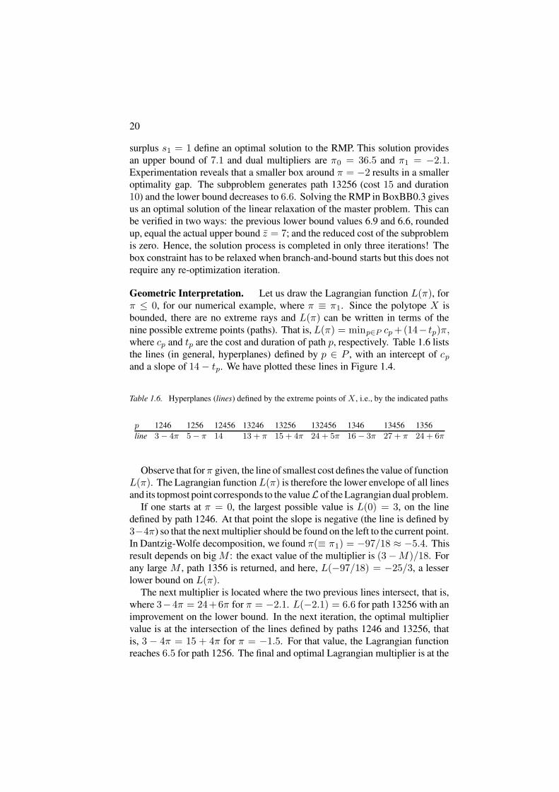
surplus s1 = 1 define an optimal solution to the RMP. This solution providesan upper bound of 7.1 and dual multipliers are π0 = 36.5 and π1 = −2.1.Experimentation reveals that a smaller box around π = −2 results in a smalleroptimality gap. The subproblem generates path 13256 (cost 15 and duration10) and the lower bound decreases to 6.6. Solving the RMP in BoxBB0.3 givesus an optimal solution of the linear relaxation of the master problem. This canbe verified in two ways: the previous lower bound values 6.9 and 6.6, roundedup, equal the actual upper bound z = 7; and the reduced cost of the subproblemis zero. Hence, the solution process is completed in only three iterations! Thebox constraint has to be relaxed when branch-and-bound starts but this does notrequire any re-optimization iteration.

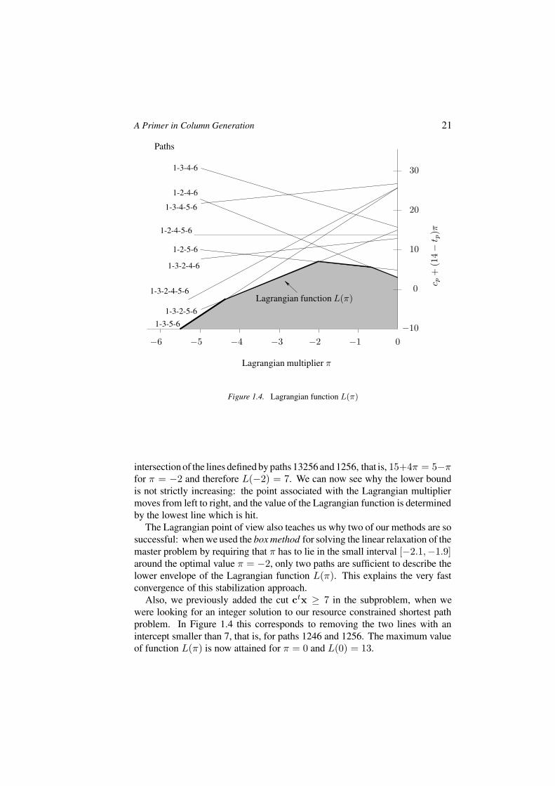
Geometric Interpretation. Let us draw the Lagrangian function L(π), forπ ≤ 0, for our numerical example, where π ≡ π1. Since the polytope X isbounded, there are no extreme rays and L(π) can be written in terms of thenine possible extreme points (paths). That is, L(π) = minp∈P cp +(14− tp)π,where cp and tp are the cost and duration of path p, respectively. Table 1.6 liststhe lines (in general, hyperplanes) defined by p ∈ P , with an intercept of cp

and a slope of 14 − tp. We have plotted these lines in Figure 1.4.

Table 1.6. Hyperplanes (lines) defined by the extreme points of X , i.e., by the indicated paths

p 1246 1256 12456 13246 13256 132456 1346 13456 1356line 3 − 4π 5 − π 14 13 + π 15 + 4π 24 + 5π 16 − 3π 27 + π 24 + 6π

Observe that for π given, the line of smallest cost defines the value of functionL(π). The Lagrangian function L(π) is therefore the lower envelope of all linesand its topmost point corresponds to the valueL of the Lagrangian dual problem.

If one starts at π = 0, the largest possible value is L(0) = 3, on the linedefined by path 1246. At that point the slope is negative (the line is defined by3−4π) so that the next multiplier should be found on the left to the current point.In Dantzig-Wolfe decomposition, we found π(≡ π1) = −97/18 ≈ −5.4. Thisresult depends on big M : the exact value of the multiplier is (3 −M)/18. Forany large M , path 1356 is returned, and here, L(−97/18) = −25/3, a lesserlower bound on L(π).

The next multiplier is located where the two previous lines intersect, that is,where 3−4π = 24+6π for π = −2.1. L(−2.1) = 6.6 for path 13256 with animprovement on the lower bound. In the next iteration, the optimal multipliervalue is at the intersection of the lines defined by paths 1246 and 13256, thatis, 3 − 4π = 15 + 4π for π = −1.5. For that value, the Lagrangian functionreaches 6.5 for path 1256. The final and optimal Lagrangian multiplier is at the


Paths

Lagrangian multiplier π

0

Lagrangian function L(π)0

c p+

(14−

t p)π

−4 −3 −2 −1−5

−10

10

20

301-3-4-6

1-2-4-6

1-3-4-5-6

1-2-4-5-6

1-2-5-6

1-3-2-4-6

1-3-2-5-6

1-3-5-6

1-3-2-4-5-6

−6

Figure 1.4. Lagrangian function L(π)

intersection of the lines defined by paths 13256 and 1256, that is, 15+4π = 5−πfor π = −2 and therefore L(−2) = 7. We can now see why the lower boundis not strictly increasing: the point associated with the Lagrangian multipliermoves from left to right, and the value of the Lagrangian function is determinedby the lowest line which is hit.

The Lagrangian point of view also teaches us why two of our methods are sosuccessful: when we used the box method for solving the linear relaxation of themaster problem by requiring that π has to lie in the small interval [−2.1,−1.9]around the optimal value π = −2, only two paths are sufficient to describe thelower envelope of the Lagrangian function L(π). This explains the very fastconvergence of this stabilization approach.

Also, we previously added the cut ctx ≥ 7 in the subproblem, when wewere looking for an integer solution to our resource constrained shortest pathproblem. In Figure 1.4 this corresponds to removing the two lines with anintercept smaller than 7, that is, for paths 1246 and 1256. The maximum valueof function L(π) is now attained for π = 0 and L(0) = 13.

22

4. On Finding a Good FormulationMany vehicle routing and crew scheduling problems, but also many others,

possess a multicommodity flow problem as an underlying basic structure (seeDesaulniers et al., 1998). Interestingly, Ford and Fulkerson, 1958, suggestedto solve this “problem of some importance in applications” via a “specializedcomputing scheme that takes advantage of the structure”: the birth of col-umn generation which then inspired Dantzig and Wolfe, 1960 to generalizethe framework to a decomposition scheme for linear programs as presented inSection 1.2.1. Ford and Fulkerson had no idea “whether the method is practica-ble.” In fact, at that time, it was not. Not only because of the lack of powerfulcomputers but mainly because (only) linear programming was used to attackinteger programs: “That integers should result as the solution of the exampleis, of course, fortuitous” (Gilmore and Gomory, 1961).

In this section we stress the importance (and the efforts) to find a “good”formulation which is amenable to column generation. Our example is theclassical column generation application, see Ben Amor and Valerio de Carvalho,2005. Given a set of rolls of width L and integer demands ni for items of lengthì, i ∈ I the aim of the cutting stock problem is to find patterns to cut the rollsto fulfill the demand while minimizing the number of used rolls. An item mayappear more than once in a cutting pattern and a cutting pattern may be usedmore than once in a feasible solution.

4.1 Gilmore and Gomory (1961, 1963)Let R be the set of all feasible cutting patterns. Let coefficient air denote how

often item i ∈ I is used in pattern r ∈ R. Feasibility of r is expressed by theknapsack constraint

∑

i∈I airì ≤ L. The classical formulation of Gilmore andGomory (1961, 1963) makes use of non-negative integer variables: λr reflectshow often pattern r is cut in the solution. We are first interested in solvingthe linear relaxation of that formulation by column generation. Consider thefollowing primal and dual linear master problems PCS and DCS , respectively:

(PCS) : min∑

r∈R λr∑

r∈R airλr ≥ ni, i ∈ Iλr ≥ 0, r ∈ R

(DCS) : max∑

i∈I niπi∑

i∈I airπi ≤ 1, r ∈ Rπi ≥ 0, i ∈ I .

For i ∈ I , let πi denote the associated dual multiplier, and let xi count thefrequency item i is selected in a pattern. Negative reduced cost patterns aregenerated by solving

min 1 −∑

i∈I

πi xi ≡ max∑

i∈I

πixi such that∑

i∈I

xiì ≤ L, xi ∈ Z+, i ∈ I.


This pricing subproblem is a knapsack problem and the coefficients of thegenerated columns are given by the value of variables xi, i ∈ I .

Gilmore and Gomory, 1961 showed that equality in the demand constraintscan be replaced by greater than or equal. Column generation is accelerated bythis transformation: dual variables πi, i ∈ I then assume only non-negativevalues and it is easily shown by contradiction that these dual non-negativityconstraints are satisfied by all optimal solutions. Therefore they define a set of(simple) dual-optimal inequalities.

Although PCS is known to provide a strong lower bound on the optimalnumber of rolls, its solution can be fractional and one has to resort to branch-and-bound. In the literature one finds several tailored branching strategies basedon decisions made on the λ variables, see Barnhart et al., 1998; Vanderbeckand Wolsey, 1996. However, we have seen that branching rules with a potentialfor exploiting more structural information can be devised when some compactformulation is available.

4.2 Kantorovich (1939, 1960)From a technical point of view, the proposal by Gilmore and Gomory is a

master problem and a pricing subproblem. For precisely this situation, Vil-leneuve et al., 2003 show that an equivalent compact formulation exists underthe assumption that the sum of the variables of the master problem be boundedby an integer κ and that we have the possibility to also bound the domain of thesubproblem. The variables and the domain of the subproblem are duplicatedκ times, and the resulting formulation has a block diagonal structure with κidentical subproblems. Formally, when we start from Gilmore and Gomory’sformulation, this yields the following formulation of the cutting stock problem.

Given the dual multipliers πi, i ∈ I , the pricing subproblem can alternativelybe written as

min (x0 −∑

i∈I

πi xi)

subject to∑

i∈I

ì xi ≤ L x0

x0 ∈ {0, 1}xi ∈ Z+ i ∈ I ,

(1.40)

where x0 is a binary variable assuming value 1 if a roll is used and 0 otherwise.When x0 is set to 1, (1.40) is equivalent to solving a knapsack problem whileif x0 = 0, then xi = 0 for all i ∈ I and this null solution corresponds to anempty pattern, i.e., a roll that is not cut.

The constructive procedure to recover a compact formulation leads to thedefinition of a specific subproblem for each roll. Let K := {1, . . . , κ} be a setof rolls of width L such that

∑

r∈R λr ≤ κ for some feasible solution λ. Let

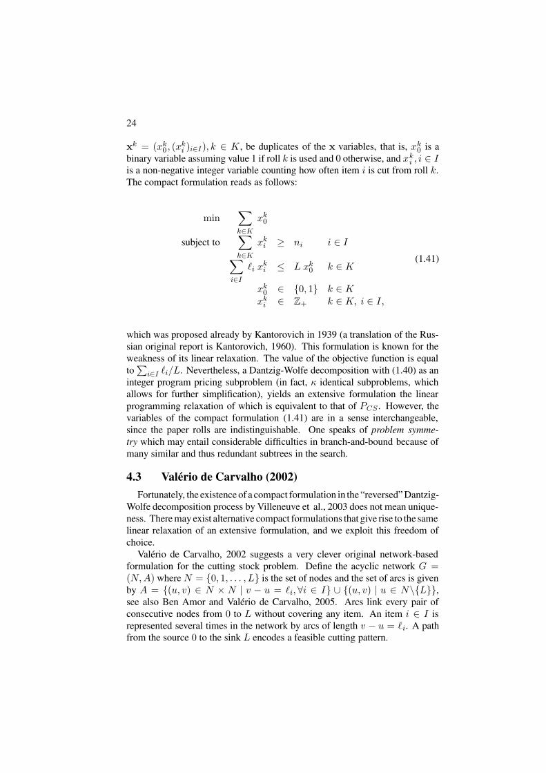
24

xk = (xk0 , (x

ki )i∈I), k ∈ K , be duplicates of the x variables, that is, xk

0 is abinary variable assuming value 1 if roll k is used and 0 otherwise, and xk

i , i ∈ Iis a non-negative integer variable counting how often item i is cut from roll k.The compact formulation reads as follows:

min∑

k∈K

xk0

subject to∑

k∈K

xki ≥ ni i ∈ I

∑

i∈I

ì xki ≤ L xk

0 k ∈ K

xk0 ∈ {0, 1} k ∈ K

xki ∈ Z+ k ∈ K, i ∈ I,

(1.41)

which was proposed already by Kantorovich in 1939 (a translation of the Rus-sian original report is Kantorovich, 1960). This formulation is known for theweakness of its linear relaxation. The value of the objective function is equalto

∑

i∈I ì/L. Nevertheless, a Dantzig-Wolfe decomposition with (1.40) as aninteger program pricing subproblem (in fact, κ identical subproblems, whichallows for further simplification), yields an extensive formulation the linearprogramming relaxation of which is equivalent to that of PCS . However, thevariables of the compact formulation (1.41) are in a sense interchangeable,since the paper rolls are indistinguishable. One speaks of problem symme-try which may entail considerable difficulties in branch-and-bound because ofmany similar and thus redundant subtrees in the search.

4.3 Valerio de Carvalho (2002)Fortunately, the existence of a compact formulation in the “reversed” Dantzig-

Wolfe decomposition process by Villeneuve et al., 2003 does not mean unique-ness. There may exist alternative compact formulations that give rise to the samelinear relaxation of an extensive formulation, and we exploit this freedom ofchoice.

Valerio de Carvalho, 2002 suggests a very clever original network-basedformulation for the cutting stock problem. Define the acyclic network G =(N,A) where N = {0, 1, . . . , L} is the set of nodes and the set of arcs is givenby A = {(u, v) ∈ N × N | v − u = ì,∀i ∈ I} ∪ {(u, v) | u ∈ N\{L}},see also Ben Amor and Valerio de Carvalho, 2005. Arcs link every pair ofconsecutive nodes from 0 to L without covering any item. An item i ∈ I isrepresented several times in the network by arcs of length v − u = ì. A pathfrom the source 0 to the sink L encodes a feasible cutting pattern.


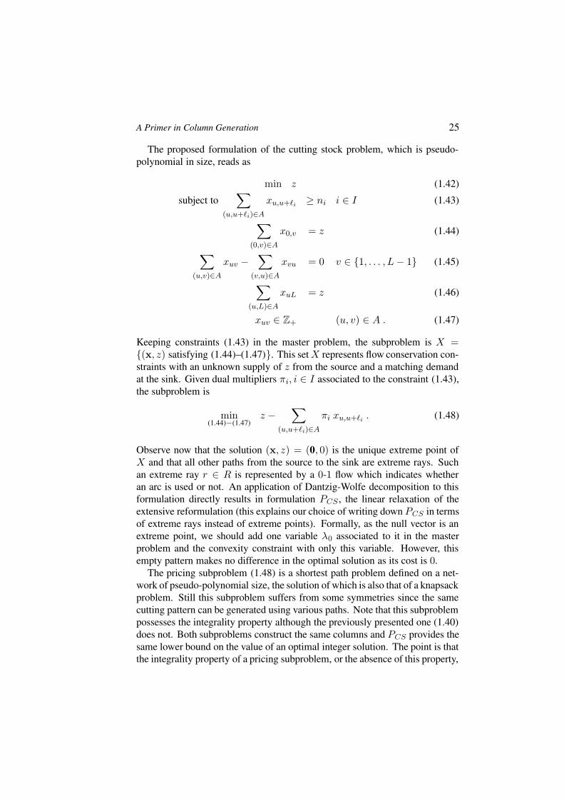
The proposed formulation of the cutting stock problem, which is pseudo-polynomial in size, reads as

min z (1.42)

subject to∑

(u,u+ì)∈A

xu,u+ì≥ ni i ∈ I (1.43)

∑

(0,v)∈A

x0,v = z (1.44)

∑

(u,v)∈A

xuv −∑

(v,u)∈A

xvu = 0 v ∈ {1, . . . , L − 1} (1.45)

∑

(u,L)∈A

xuL = z (1.46)

xuv ∈ Z+ (u, v) ∈ A . (1.47)

Keeping constraints (1.43) in the master problem, the subproblem is X ={(x, z) satisfying (1.44)–(1.47)}. This set X represents flow conservation con-straints with an unknown supply of z from the source and a matching demandat the sink. Given dual multipliers πi, i ∈ I associated to the constraint (1.43),the subproblem is

min(1.44)−(1.47)

z −∑

(u,u+ì)∈A

πi xu,u+ì. (1.48)

Observe now that the solution (x, z) = (0, 0) is the unique extreme point ofX and that all other paths from the source to the sink are extreme rays. Suchan extreme ray r ∈ R is represented by a 0-1 flow which indicates whetheran arc is used or not. An application of Dantzig-Wolfe decomposition to thisformulation directly results in formulation PCS , the linear relaxation of theextensive reformulation (this explains our choice of writing down PCS in termsof extreme rays instead of extreme points). Formally, as the null vector is anextreme point, we should add one variable λ0 associated to it in the masterproblem and the convexity constraint with only this variable. However, thisempty pattern makes no difference in the optimal solution as its cost is 0.

The pricing subproblem (1.48) is a shortest path problem defined on a net-work of pseudo-polynomial size, the solution of which is also that of a knapsackproblem. Still this subproblem suffers from some symmetries since the samecutting pattern can be generated using various paths. Note that this subproblempossesses the integrality property although the previously presented one (1.40)does not. Both subproblems construct the same columns and PCS provides thesame lower bound on the value of an optimal integer solution. The point is thatthe integrality property of a pricing subproblem, or the absence of this property,

26

has to be evaluated relative to its own compact formulation. In the present case,the linear relaxation of Kantorovich’s formulation provides a lower bound thatis weaker than that of PCS , although it can be improved by solving the integerknapsack pricing subproblem (1.40). On the other hand, the linear relaxationof Valerio de Carvalho’s formulation already provides the same lower boundas PCS . Using this original formulation, one can design branching and cut-ting decisions on the arc flow variables of network G to get an optimal integersolution.

Let us mention that there are many important applications which have anatural formulation as set covering or set partitioning problems, without anydecomposition. In such models it is usually the master problem itself which hasto be solved in integers (Barnhart et al., 1998). Even though there is no explicitoriginal formulation used, customized branching rules can often be interpretedas branching on variables of such a formulation.

5. Further ReadingEven though column generation originates from linear programming, its

strengths unfold in solving integer programming problems. The simultaneoususe of two concurrent formulations, compact and extensive, allows for a betterunderstanding of the problem at hand and stimulates our inventiveness in whatconcerns for example branching rules.

We have said only little about implementation issues, but there would beplenty to discuss. Every ingredient of the process deserves its own attention,see e.g., Desaulniers et al., 2001, who collect a wealth of acceleration ideas andshare their experience. Clearly, an implementation benefits from customizationto a particular application. Still, it is our impression that an off-the-shelf columngeneration software to solve large scale integer programs is in reach reasonablysoon; the necessary building blocks are already available. A crucial part is toautomatically detect how to “best” decompose a given original formulation,see Vanderbeck, 2005. This means in particular exploiting the absence ofthe subproblem’s integrality property, if applicable, since this may reduce theintegrality gap without negative consequences for the linear master program.Let us also remark that instead of a convexification of the subproblem’s domainX (when bounded), one can explicitly represent all integer points in X via adiscretization approach formulated by Vanderbeck, 2000. The decompositionthen leads to a master problem which itself has to be solved in integer variables.

In what regards new and important technical developments, in addition to thestabilization of dual variables already mentioned, one can find a dynamic rowaggregation technique for set partitioning master problems in Elhallaoui et al.,2003. This allows for a considerable reduction in size of the restricted masterproblem in each iteration. An interesting approach is also proposed by Valerio


de Carvalho, 1999 where variables and rows of the original formulation aredynamically generated from the solutions of the subproblem. This techniqueexploits the fact that the subproblem possesses the integrality property. Fora presentation of this idea in the context of a multicommodity network flowproblem we refer to Mamer and McBride, 2000.

This primer is based on our recent survey (Lubbecke and Desrosiers, 2002),and a much more detailed presentation and over one hundred references can befound there. For those interested in the many column generation applicationsin practice, the survey articles in this book will serve the reader as entry pointsto the large body of literature. Last, but not least, we recommend the book byLasdon, 1970, also in its recent second edition, as an indispensable source foralternative methods of decomposition.

Acknowledgments. We would like to thank Steffen Rebennack for cross-checking our numerical example, and Marcus Poggi de Aragao, Eduardo Uchoa,Geir Hasle, and Jose Manuel Valerio de Carvalho, and the two referees forgiving us useful feedback on an earlier draft of this chapter. This research wassupported in part by an NSERC grant for the first author.

ReferencesAhuja, R.K., Magnanti, T.L., and Orlin, J.B. (1993). Network Flows: Theory,

Algorithms and Applications. Prentice-Hall, Inc., Englewood Cliffs, NewJersey 07632.

Barnhart, C., Johnson, E.L., Nemhauser, G.L., Savelsbergh, M.W.P., and Vance,P.H. (1998). Branch-and-price: Column generation for solving huge integerprograms. Oper. Res., 46(3):316–329.

Ben Amor, H. and Desrosiers, J. (2003) A Proximal Trust Region Algorithmfor Column Generation Stabilization. Les Cahiers du GERAD G-2003-43(2003). To appear in Comp. & OR.

Ben Amor, H., Desrosiers, J., and Valerio de Carvalho, J.M. (2003). Dual-optimal inequalities for stabilized column generation. Les Cahiers du GERADG-2003-20, HEC Montreal. Under revision for Oper. Res.

Ben Amor, H. and Valerio de Carvalho, J.M. (2005). Cutting stock problems. InDesaulniers, G., Desrosiers, J., and Solomon, M.M., editors, Column Gen-eration. Kluwer Academic Publishers, Boston, MA.

Dantzig, G.B. and Wolfe, P. (1960). Decomposition principle for linear pro-grams. Oper. Res., 8:101–111.

Desaulniers, G., Desrosiers, J., Ioachim, I., Solomon, M.M., Soumis, F., and Vil-leneuve, D. (1998). A unified framework for deterministic time constrainedvehicle routing and crew scheduling problems. In Crainic, T.G. and Laporte,G., editors, Fleet Management and Logistics, pages 57–93. Kluwer, Norwell,MA.

28

Desaulniers, G., Desrosiers, J., and Solomon, M.M. (2001). Accelerating strate-gies in column generation methods for vehicle routing and crew schedulingproblems. In Ribeiro, C.C. and Hansen, P., editors, Essays and Surveys inMetaheuristics, pages 309–324, Boston. Kluwer.

du Merle, O., Villeneuve, D., Desrosiers, J., and Hansen, P. (1999). Stabilizedcolumn generation. Discrete Math., 194:229–237.

Elhallaoui, I., Villeneuve, D., Soumis, F., and Desaulniers, G. (2003). Dynamicaggregation of set partitioning constraints in column generation. Les Cahiersdu GERAD G-2003-45, HEC Montreal. Under revision for Oper. Res.

Ford, L.R. and Fulkerson, D.R. (1958). A suggested computation for maximalmulticommodity network flows. Management Sci., 5:97–101.

Geoffrion, A.M. (1974). Lagrangean relaxation for integer programming. Math.Programming Stud., 2:82–114.

Gilmore, P.C. and Gomory, R.E. (1961). A linear programming approach to thecutting-stock problem. Oper. Res., 9:849–859.

Gilmore, P.C. and Gomory, R.E. (1963). A linear programming approach to thecutting stock problem—Part II. Oper. Res., 11:863–888.

Goffin, J.-L. and Vial, J.-Ph. (1999). Convex nondifferentiable optimization:A survey focussed on the analytic center cutting plane method. TechnicalReport 99.02, Logilab, Universite de Geneve. To appear in Optim. MethodsSoftw.

Guignard, M. (2004). Lagrangean relaxation. In Resende, M. and Pardalos, P.,editors, Handbook of Applied Optimization. Oxford University Press.

Hiriart-Urruty, J.-B. and Lemarechal, C. (1993). Convex analysis and minimiza-tion algorithms, part 2: Advanced theory and bundle methods, volume 306of Grundlehren der mathematischen Wissenschaften. Springer, Berlin.

Kantorovich, L. (1960). Mathematical methods of organising and planning pro-duction (translated from a report in russian, dated 1939). Management Sci-ence, 6:366–422.

Kelley Jr., J.E. (1961). The cutting-plane method for solving convex programs.J. Soc. Ind. Appl. Math., 8(4):703–712.

Lasdon, L.S. (1970). Optimization Theory for Large Systems. Macmillan, Lon-don.

Lubbecke, M.E. and Desrosiers, J. (2002). Selected topics in column generation.Les Cahiers du GERAD G-2002-64, HEC Montreal. Under revision for Oper.Res.

Nemhauser, G.L. and Wolsey, L.A. (1988), Integer and Combinatorial Opti-mization. John Wiley & Sons, Chichester.

Mamer, J.W. and McBride, R.D. (2000). A decomposition-based pricing pro-cedure for large-scale linear programs – An application to the linear multi-commodity flow problem. Management Sci., 46(5):693–709.


Marsten, R.E. (1975). The use of the boxstep method in discrete optimization.Math. Programming Stud., 3:127–144.

Marsten, R.E., Hogan, W.W., and Blankenship, J.W. (1975). The Boxstep

method for large-scale optimization. Oper. Res., 23:389–405.Poggi de Aragao, M. and Uchoa, E. (2003). Integer program reformulation

for robust branch-and-cut-and-price algorithms. In Proceedings of the Con-ference Mathematical Program in Rio: A Conference in Honour of NelsonMaculan, pages 56–61.

Schrijver, A. (1986). Theory of Linear and Integer Programming. John Wiley& Sons, Chichester.

Valerio de Carvalho, J.M. (1999). Exact solution of bin-packing problems usingcolumn generaion and branch-and-bound. Annals of Operations Research,86:629–659.

Valerio de Carvalho, J.M. (2002). LP models for bin-packing and cutting stockproblems. European J. Oper. Res., 141(2):253–273.

Valerio de Carvalho, J.M. (2003). Using extra dual cuts to accelerate conver-gence in column generation. To appear in INFORMS J. Comput.

Vanderbeck, F. (2000). On Dantzig-Wolfe decomposition in integer program-ming and ways to perform branching in a branch-and-price algorithm. Oper.Res., 48(1):111–128.

Vanderbeck, F. (2005). Implementing mixed integer column generation. In De-saulniers, G., Desrosiers, J., and Solomon, M.M., editors, Column Genera-tion. Kluwer Academic Publishers, Boston, MA.

Vanderbeck, F. and Wolsey, L.A. (1996). An exact algorithm for IP columngeneration. Oper. Res. Lett., 19:151–159.

Villeneuve, D., Desrosiers, J., Lubbecke, M.E., and Soumis, F. (2003). Oncompact formulations for integer programs solved by column generation.Les Cahiers du GERAD G-2003-06, HEC Montreal. To appear in Ann. Oper.Res.

Walker, W.E. (1969). A method for obtaining the optimal dual solution to a linearprogram using the Dantzig-Wolfe decomposition. Oper. Res., 17:368–370.

Documents

Chapter 1 · Chapter 1 A PRIMER IN COLUMN ... linear and in particular in integer programming. We touch on both, ... BB0: The linear programming relaxation of the master problem