Embed Size (px)
Citation preview
PART 4
WAVES ANDAPPLICATIONS
Chapter y
MAXWELL'S EQUATIONS
Do you want to be a hero? Don't be the kind of person who watches others do
great things or doesn't know what's happening. Go out and make things happen.
The people who get things done have a burning desire to make things happen, get
ahead, serve more people, become the best they can possibly be, and help
improve the world around them.
—GLENN VAN EKEREN
9.1 INTRODUCTION
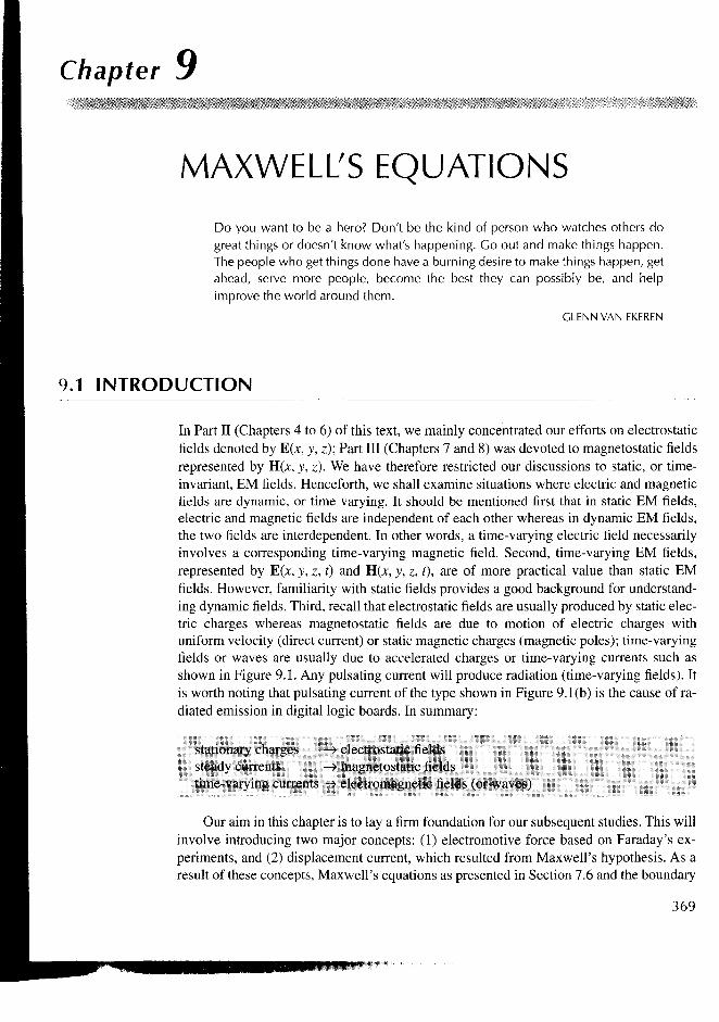
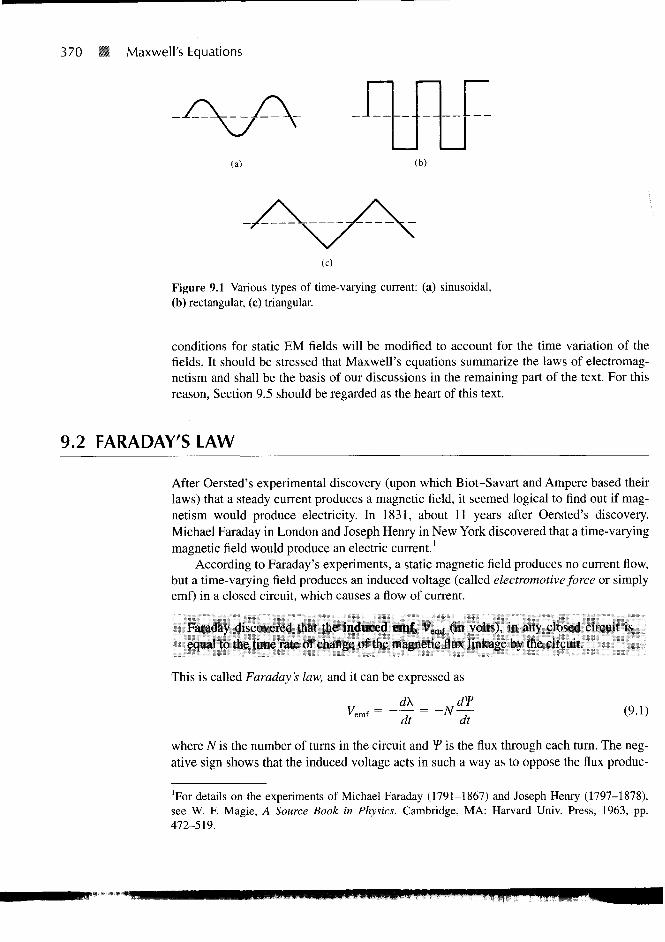
In Part II (Chapters 4 to 6) of this text, we mainly concentrated our efforts on electrostaticfields denoted by E(x, y, z); Part III (Chapters 7 and 8) was devoted to magnetostatic fieldsrepresented by H(JC, y, z). We have therefore restricted our discussions to static, or time-invariant, EM fields. Henceforth, we shall examine situations where electric and magneticfields are dynamic, or time varying. It should be mentioned first that in static EM fields,electric and magnetic fields are independent of each other whereas in dynamic EM fields,the two fields are interdependent. In other words, a time-varying electric field necessarilyinvolves a corresponding time-varying magnetic field. Second, time-varying EM fields,represented by E(x, y, z, t) and H(x, y, z, t), are of more practical value than static EMfields. However, familiarity with static fields provides a good background for understand-ing dynamic fields. Third, recall that electrostatic fields are usually produced by static elec-tric charges whereas magnetostatic fields are due to motion of electric charges withuniform velocity (direct current) or static magnetic charges (magnetic poles); time-varyingfields or waves are usually due to accelerated charges or time-varying currents such asshown in Figure 9.1. Any pulsating current will produce radiation (time-varying fields). Itis worth noting that pulsating current of the type shown in Figure 9.1(b) is the cause of ra-diated emission in digital logic boards. In summary:
charges —> electrostatic fieldssteady currenis —» magnclosiatic fieldstime-varying currenis ••» electromagnetic fields (or wavesj
Our aim in this chapter is to lay a firm foundation for our subsequent studies. This willinvolve introducing two major concepts: (1) electromotive force based on Faraday's ex-periments, and (2) displacement current, which resulted from Maxwell's hypothesis. As aresult of these concepts, Maxwell's equations as presented in Section 7.6 and the boundary
369
370 Maxwell's Equations
(a) (b)
(0
Figure 9.1 Various types of time-varying current: (a) sinusoidal,(b) rectangular, (c) triangular.
conditions for static EM fields will be modified to account for the time variation of thefields. It should be stressed that Maxwell's equations summarize the laws of electromag-netism and shall be the basis of our discussions in the remaining part of the text. For thisreason, Section 9.5 should be regarded as the heart of this text.
9.2 FARADAY'S LAW
After Oersted's experimental discovery (upon which Biot-Savart and Ampere based theirlaws) that a steady current produces a magnetic field, it seemed logical to find out if mag-netism would produce electricity. In 1831, about 11 years after Oersted's discovery,Michael Faraday in London and Joseph Henry in New York discovered that a time-varyingmagnetic field would produce an electric current.'
According to Faraday's experiments, a static magnetic field produces no current flow,but a time-varying field produces an induced voltage (called electromotive force or simplyemf) in a closed circuit, which causes a flow of current.
Faraday discovered that the induced emf. \\.iM (in volts), in any closed circuit isequal to the time rale of change of the magnetic flux linkage by the circuit.
This is called Faraday's law, and it can be expressed as
dt dt• e m f (9.1)
where N is the number of turns in the circuit and V is the flux through each turn. The neg-ative sign shows that the induced voltage acts in such a way as to oppose the flux produc-
'For details on the experiments of Michael Faraday (1791-1867) and Joseph Henry (1797-1878),see W. F. Magie, A Source Book in Physics. Cambridge, MA: Harvard Univ. Press, 1963, pp.472-519.
9.2 FARADAY'S LAW 371
battery
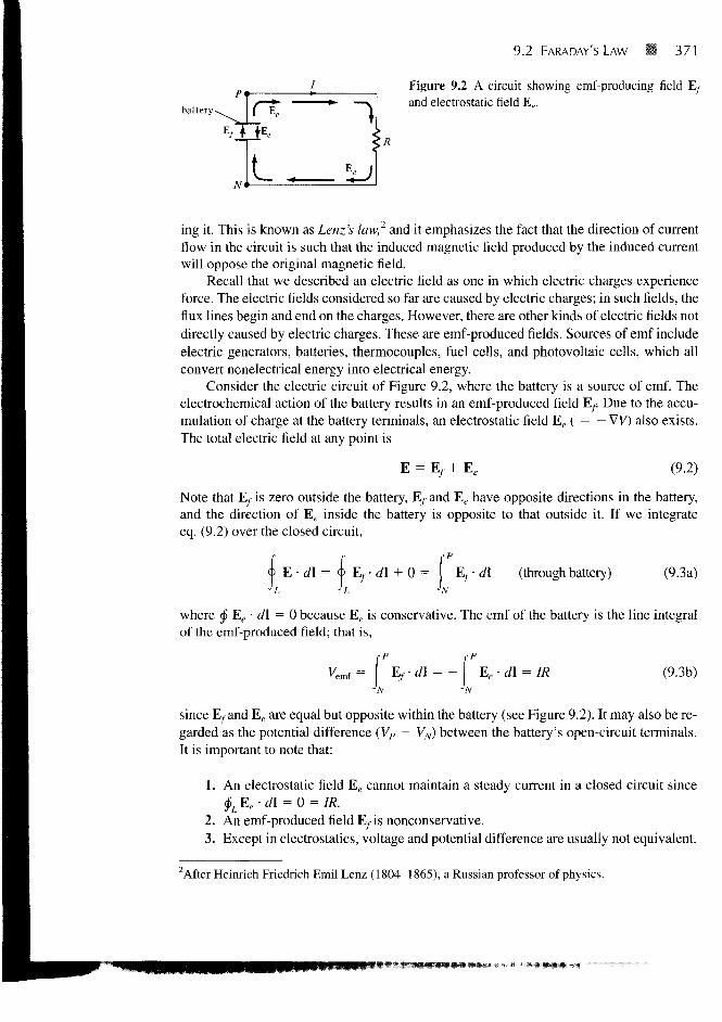
Figure 9.2 A circuit showing emf-producing fieldand electrostatic field E,.
ing it. This is known as Lenz's law,2 and it emphasizes the fact that the direction of currentflow in the circuit is such that the induced magnetic field produced by the induced currentwill oppose the original magnetic field.
Recall that we described an electric field as one in which electric charges experienceforce. The electric fields considered so far are caused by electric charges; in such fields, theflux lines begin and end on the charges. However, there are other kinds of electric fields notdirectly caused by electric charges. These are emf-produced fields. Sources of emf includeelectric generators, batteries, thermocouples, fuel cells, and photovoltaic cells, which allconvert nonelectrical energy into electrical energy.
Consider the electric circuit of Figure 9.2, where the battery is a source of emf. Theelectrochemical action of the battery results in an emf-produced field Ey. Due to the accu-mulation of charge at the battery terminals, an electrostatic field Ee{ = — VV) also exists.The total electric field at any point is
E = Ey + Ee (9.2)
Note that Ey is zero outside the battery, Ey and Ee have opposite directions in the battery,and the direction of Ee inside the battery is opposite to that outside it. If we integrateeq. (9.2) over the closed circuit,
E • d\ = <f Ey • d\ + 0 = Ef-dl (through battery) (9.3a)
where § Ee • d\ = 0 because Ee is conservative. The emf of the battery is the line integralof the emf-produced field; that is,
d\ = - (9.3b)
since Eyand Ee are equal but opposite within the battery (see Figure 9.2). It may also be re-garded as the potential difference (VP - VN) between the battery's open-circuit terminals.It is important to note that:
1. An electrostatic field Ee cannot maintain a steady current in a closed circuit since$LEe-dl = 0 = //?.
2. An emf-produced field Eyis nonconservative.3. Except in electrostatics, voltage and potential difference are usually not equivalent.
2After Heinrich Friedrich Emil Lenz (1804-1865), a Russian professor of physics.
372 B Maxwell's Equations
9.3 TRANSFORMER AND MOTIONAL EMFs
Having considered the connection between emf and electric field, we may examine howFaraday's law links electric and magnetic fields. For a circuit with a single turn (N = 1),eq. (9.1) becomes
V - ** (9.4)
In terms of E and B, eq. (9.4) can be written as
yemf = f E • d\ = - - Bh dt 4
(9.5)
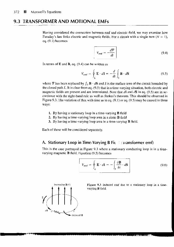
where *P has been replaced by Js B • dS and S is the surface area of the circuit bounded bythe closed path L. It is clear from eq. (9.5) that in a time-varying situation, both electric andmagnetic fields are present and are interrelated. Note that d\ and JS in eq. (9.5) are in ac-cordance with the right-hand rule as well as Stokes's theorem. This should be observed inFigure 9.3. The variation of flux with time as in eq. (9.1) or eq. (9.5) may be caused in threeways:
1. By having a stationary loop in a time-varying B field2. By having a time-varying loop area in a static B field3. By having a time-varying loop area in a time-varying B field.
Each of these will be considered separately.
A. Stationary Loop in Time-Varying B Fit transformer emf)
This is the case portrayed in Figure 9.3 where a stationary conducting loop is in a time-varying magnetic B field. Equation (9.5) becomes
(9.6)
Increasing B(t) Figure 9.3 Induced emf due to a stationary loop in a time-varying B field.
:ed B
9.3 TRANSFORMER AND MOTIONAL EMFS 373
This emf induced by the time-varying current (producing the time-varying B field) in a sta-tionary loop is often referred to as transformer emf in power analysis since it is due totransformer action. By applying Stokes's theorem to the middle term in eq. (9.6), we obtain
(V X E) • dS = - I — • dS
For the two integrals to be equal, their integrands must be equal; that is,
(9.7)
dt(9.8)
This is one of the Maxwell's equations for time-varying fields. It shows that the time-varying E field is not conservative (V X E + 0). This does not imply that the principles ofenergy conservation are violated. The work done in taking a charge about a closed path ina time-varying electric field, for example, is due to the energy from the time-varying mag-netic field. Observe that Figure 9.3 obeys Lenz's law; the induced current / flows such asto produce a magnetic field that opposes B(f).
B. Moving Loop in Static B Field (Motional emf)
When a conducting loop is moving in a static B field, an emf is induced in the loop. Werecall from eq. (8.2) that the force on a charge moving with uniform velocity u in a mag-netic field B is
Fm = Qu X B
We define the motional electric field Em as
(8.2)
Em = - ^ = u X B (9.9)
If we consider a conducting loop, moving with uniform velocity u as consisting of a largenumber of free electrons, the emf induced in the loop is
(9.10)
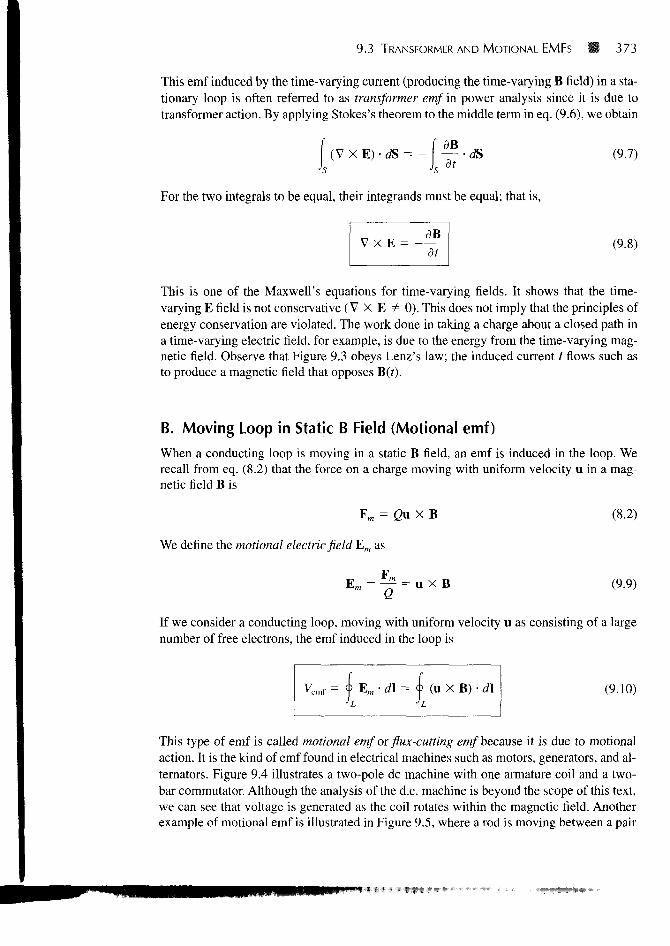
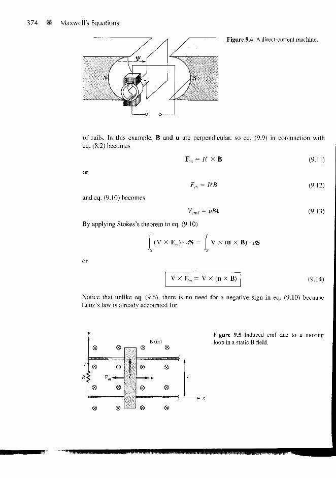
This type of emf is called motional emf or flux-cutting emf because it is due to motionalaction. It is the kind of emf found in electrical machines such as motors, generators, and al-ternators. Figure 9.4 illustrates a two-pole dc machine with one armature coil and a two-bar commutator. Although the analysis of the d.c. machine is beyond the scope of this text,we can see that voltage is generated as the coil rotates within the magnetic field. Anotherexample of motional emf is illustrated in Figure 9.5, where a rod is moving between a pair
374 11 Maxwell's Equations
Figure 9.4 A direct-current machine.
of rails. In this example, B and u are perpendicular, so eq. (9.9) in conjunction witheq. (8.2) becomes
or
and eq. (9.10) becomes
Fm = U X B
Fm = KB
Vem( =
By applying Stokes's theorem to eq. (9.10)
( V X E J ' d S = V X (u X B) • dS's 's
or
V X Em = V X (u X B)
(9.11)
(9.12)
(9.13)
(9.14)
Notice that unlike eq. (9.6), there is no need for a negative sign in eq. (9.10) becauseLenz's law is already accounted for.
B(in)Figure 9.5 Induced emf due to a movingloop in a static B field.
9.3 TRANSFORMER AND MOTIONAL EMFS 375
To apply eq. (9.10) is not always easy; some care must be exercised. The followingpoints should be noted:
1. The integral in eq. (9.10) is zero along the portion of the loop where u = 0. Thusd\ is taken along the portion of the loop that is cutting the field (along the rod inFigure 9.5), where u has nonzero value.
2. The direction of the induced current is the same as that of Em or u X B. The limitsof the integral in eq. (9.10) are selected in the opposite direction to the inducedcurrent thereby satisfying Lenz's law. In eq. (9.13), for example, the integrationover L is along —av whereas induced current flows in the rod along ay.
C. Moving Loop in Time-Varying Field
This is the general case in which a moving conducting loop is in a time-varying magneticfield. Both transformer emf and motional emf are present. Combining eqs. (9.6) and (9.10)gives the total emf as
(9.15)f
V f = 9J E •d\ =f flB ft (u X B) •d\
or from eqs. (9.8) and (9.14),
V X E = + V X (u X B)dt
(9.16)
Note that eq. (9.15) is equivalent to eq. (9.4), so Vemf can be found using either eq. (9.15)or (9.4). In fact, eq. (9.4) can always be applied in place of eqs. (9.6), (9.10), and (9.15).
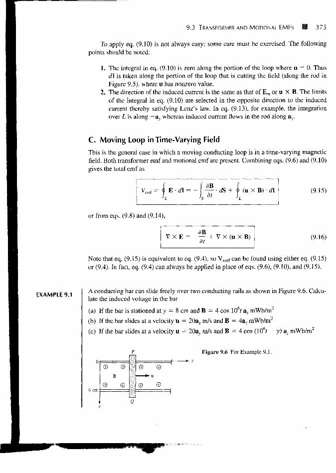
EXAMPLE 9.1A conducting bar can slide freely over two conducting rails as shown in Figure 9.6. Calcu-late the induced voltage in the bar
(a) If the bar is stationed at y = 8 cm and B = 4 cos 106f az mWb/m2
(b) If the bar slides at a velocity u = 20aj, m/s and B = 4az mWb/m2
(c) If the bar slides at a velocity u = 20ay m/s and B = 4 cos (106r — y) az mWb/m2
Figure 9.6 For Example 9.1.
0
6 cm
©
©B
©
©
0 ©
0 ©
376 Maxwell's Equations
Solution:
(a) In this case, we have transformer emf given by
dB
dtdS =
0.08 /-0.06
y=0
sin Wtdxdy
= 4(103)(0.08)(0.06) sin l06t= 19.2 sin 106;V
The polarity of the induced voltage (according to Lenz's law) is such that point P on thebar is at lower potential than Q when B is increasing.
(b) This is the case of motional emf:
Vemf = (" x B) • d\ = {u&y X Baz) • dxax
= -uB( = -20(4.10"3)(0.06)= -4.8 mV
(c) Both transformer emf and motional emf are present in this case. This problem can besolved in two ways.
Method 1: Using eq. (9.15)
Kmf = " I — • dS + | (U X B) • d\
r0.06 ry
(9.1.1)
x=0 ""00
[20ay X 4.10 3 cos(106f - y)aj • dxax
0.06
= 240 cos(106f - / ) - 80(10~3)(0.06) cos(106r - y)
= 240 008(10"? - y) - 240 cos 106f - 4.8(10~j) cos(106f - y)=- 240 cos(106f -y)- 240 cos 106? (9.1.2)
because the motional emf is negligible compared with the transformer emf. Using trigono-metric identity
A + B A - Bcos A - cos B = - 2 sin sin — - —
Veirf = 480 sin MO6? - £ ) sin ^ V (9.1.3)
9.3 TRANSFORMER AND MOTIONAL EMFS
Method 2: Alternatively we can apply eq. (9.4), namely,
Vemt = ~
where
dt
377
(9.1.4)
B-dS
•0.06
4 cos(106r - y) dx dyy=0 JJt=
= -4(0.06) sin(106f - y)
= -0.24 sin(106r - y) + 0.24 sin 10°f mWb
But
Hence,
— = u -> y = ut = 20/
V = -0.24 sin(106r - 200 + 0.24 sin 106f mWb
yemf = = 0.24(106 - 20) cos(106r - 20f) - 0.24(106) cos 106f mVdt
= 240 cos(106f - y) - 240 cos 106f V (9.1.5)
which is the same result in (9.1.2). Notice that in eq. (9.1.1), the dependence of y on timeis taken care of in / (u X B) • d\, and we should not be bothered by it in dB/dt. Why?Because the loop is assumed stationary when computing the transformer emf. This is asubtle point one must keep in mind in applying eq. (9.1.1). For the same reason, the secondmethod is always easier.
PRACTICE EXERCISE 9.1
Consider the loop of Figure 9.5. If B = 0.5az Wb/m2, R = 20 0, € = 10 cm, and therod is moving with a constant velocity of 8ax m/s, find
(a) The induced emf in the rod
(b) The current through the resistor
(c) The motional force on the rod
(d) The power dissipated by the resistor.
Answer: (a) 0.4 V, (b) 20 mA, (c) - a x mN, (d) 8 mW.
378 • Maxwell's Equations
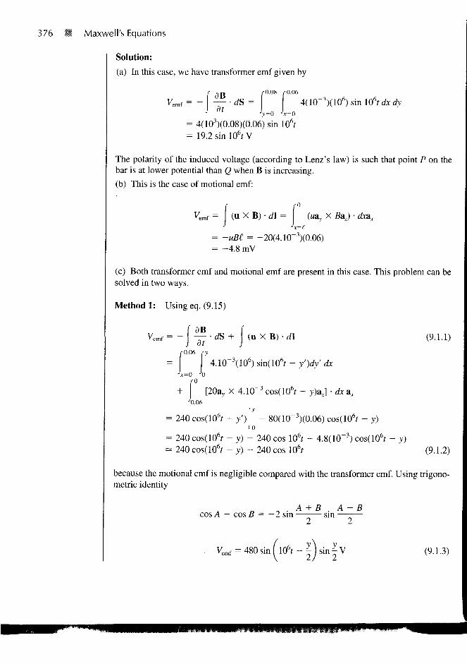
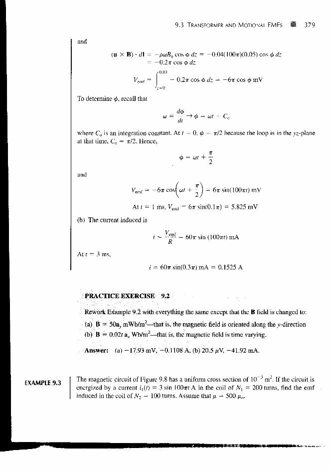
EXAMPLE 9.2The loop shown in Figure 9.7 is inside a uniform magnetic field B = 50 ax mWb/m2. Ifside DC of the loop cuts the flux lines at the frequency of 50 Hz and the loop lies in thejz-plane at time t = 0, find
(a) The induced emf at t = 1 ms
(b) The induced current at t = 3 ms
Solution:
(a) Since the B field is time invariant, the induced emf is motional, that is,
yemf = (u x B) • d\
where
d\ = d\DC = dzaz, u =dt dt
p = AD = 4 cm, a) = 2TT/ = IOOTT
As u and d\ are in cylindrical coordinates, we transform B into cylindrical coordinatesusing eq. (2.9):
B = BQax = Bo (cos <j> ap - sin <t> a0)
where Bo = 0.05. Hence,
u X B = 0 pco 0Bo cos 4> —Bo sin 4> 0
= —puBo cos </> az
Figure 9.7 For Example 9.2; polarity is forincreasing emf.
9.3 TRANSFORMER AND MOTIONAL EMFS • 379
and
(uXB)-dl= -puBo cos <f> dz = - 0 . 0 4 ( 1 0 0 T T ) ( 0 . 0 5 ) COS <t> dz= —0.2-ir cos 0 dz
r 0.03
V e m f = — 0 .2TT COS 4> dz = — 6TT COS <f> m V4=0
To determine <j>, recall that
d<t>co = > 0 = cof + C odt
where Co is an integration constant. At t = 0, 0 = TT/2 because the loop is in the yz-planeat that time, Co = TT/2. Hence,
= CO/ +TT
and
mf = ~6TT cosf cor + — ) = 6TT sin(lOOirf) mV
At f = 1 ms, yemf = 6TT sin(O.lTr) = 5.825 mV
(b) The current induced is
. Vem{
R= 607rsin(100xr)mA
At t = 3 ms,
i = 60TT sin(0.37r) mA = 0.1525 A
PRACTICE EXERCISE 9.2
Rework Example 9.2 with everything the same except that the B field is changed to:
(a) B = 50av. mWb/m2—that is, the magnetic field is oriented along the y-direction
(b) B = 0.02ir ax Wb/m2—that is, the magnetic field is time varying.
Answer: (a) -17.93 mV, -0.1108 A, (b) 20.5 jtV, -41.92 mA.
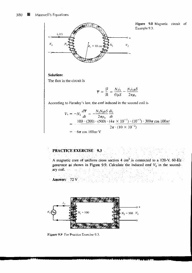
EXAMPLE 9.3The magnetic circuit of Figure 9.8 has a uniform cross section of 10 3 m2. If the circuit isenergized by a current ix{i) = 3 sin IOOTT? A in the coil of N\ = 200 turns, find the emfinduced in the coil of N2 = 100 turns. Assume that JX. = 500 /xo.
380 11 Maxwell's Equations
/Ah(o / r
" l lpo = 10 cm <LJN2
<Dl\
Solution:
The flux in the circuit is
w — —
Figure 9.8 Magnetic circuit ofExample 9.3.
-o +
2irpo
According to Faraday's law, the emf induced in the second coil is
V2 = -N2 —r = — ~ -dt 2-Kp0 dt
100 • (200) • (500) • (4TT X 10"7) • (10~3) • 300TT COS IOOTT?
2x • (10 X 10"2)= -6TTCOS 100ir?V
PRACTICE EXERCISE 9.3
A magnetic core of uniform cross section 4 cm2 is connected to a 120-V, 60-Hzgenerator as shown in Figure 9.9. Calculate the induced emf V2 in the second-ary coil.
Aaswer: 72 V
Vtfc)
Ti
> N2 = 300 V2
Figure 9.9 For Practice Exercise 9.3.
9.4 DISPLACEMENT CURRENT 381
9.4 DISPLACEMENT CURRENT
In the previous section, we have essentially reconsidered Maxwell's curl equation for elec-trostatic fields and modified it for time-varying situations to satisfy Faraday's law. We shallnow reconsider Maxwell's curl equation for magnetic fields (Ampere's circuit law) fortime-varying conditions.
For static EM fields, we recall that
V x H = J (9.17)
But the divergence of the curl of any vector field is identically zero (see Example 3.10).Hence,
V - ( V X H ) = 0 = V - J
The continuity of current in eq. (5.43), however, requires that
(9.18)
(9.19)
Thus eqs. (9.18) and (9.19) are obviously incompatible for time-varying conditions. Wemust modify eq. (9.17) to agree with eq. (9.19). To do this, we add a term to eq. (9.17) sothat it becomes
V X H = J + Jd (9.20)
where id is to be determined and defined. Again, the divergence of the curl of any vector iszero. Hence:
In order for eq. (9.21) to agree with eq. (9.19),
(9.21)
(9.22a)
or
h
3.20) results
V X H =
dD
dt
in
.1 +dX)
dt
(9.22b)
(9.23)
This is Maxwell's equation (based on Ampere's circuit law) for a time-varying field. Theterm Jd = dD/dt is known as displacement current density and J is the conduction current
382 • Maxwell's Equations
(a)
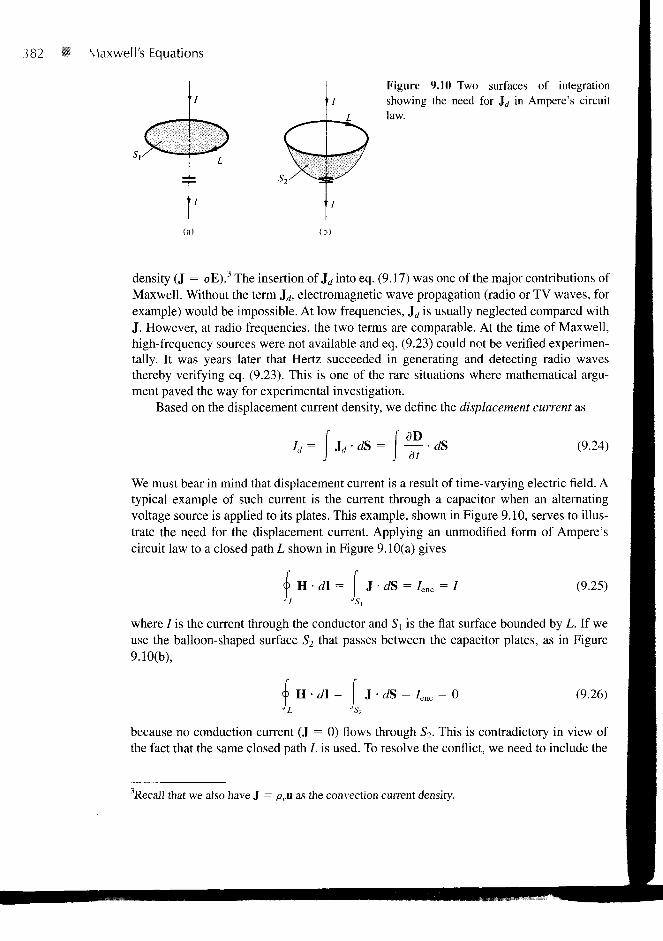
Figure 9.10 Two surfaces of integration/ showing the need for Jd in Ampere's circuit
law.
density (J = aE).3 The insertion of Jd into eq. (9.17) was one of the major contributions ofMaxwell. Without the term Jd, electromagnetic wave propagation (radio or TV waves, forexample) would be impossible. At low frequencies, Jd is usually neglected compared withJ. However, at radio frequencies, the two terms are comparable. At the time of Maxwell,high-frequency sources were not available and eq. (9.23) could not be verified experimen-tally. It was years later that Hertz succeeded in generating and detecting radio wavesthereby verifying eq. (9.23). This is one of the rare situations where mathematical argu-ment paved the way for experimental investigation.
Based on the displacement current density, we define the displacement current as
ld= \jd-dS =dt
dS (9.24)
We must bear in mind that displacement current is a result of time-varying electric field. Atypical example of such current is the current through a capacitor when an alternatingvoltage source is applied to its plates. This example, shown in Figure 9.10, serves to illus-trate the need for the displacement current. Applying an unmodified form of Ampere'scircuit law to a closed path L shown in Figure 9.10(a) gives
(9.25)H d\ = J • dS = /enc = /
where / is the current through the conductor and Sx is the flat surface bounded by L. If weuse the balloon-shaped surface S2 that passes between the capacitor plates, as in Figure9.10(b),
(9.26)H d\ = J • dS = Ieac = 0
4because no conduction current (J = 0) flows through S2- This is contradictory in view ofthe fact that the same closed path L is used. To resolve the conflict, we need to include the
• Recall that we also have J = pvii as the convection current density.
9.4 DISPLACEMENT CURRENT 383
displacement current in Ampere's circuit law. The total current density is J + Jd. Ineq. (9.25), id = 0 so that the equation remains valid. In eq. (9.26), J = 0 so that
H d\ = I id • dS = =- I D • dS = -~ = Idt dt
(9.27)
So we obtain the same current for either surface though it is conduction current in S{ anddisplacement current in S2.
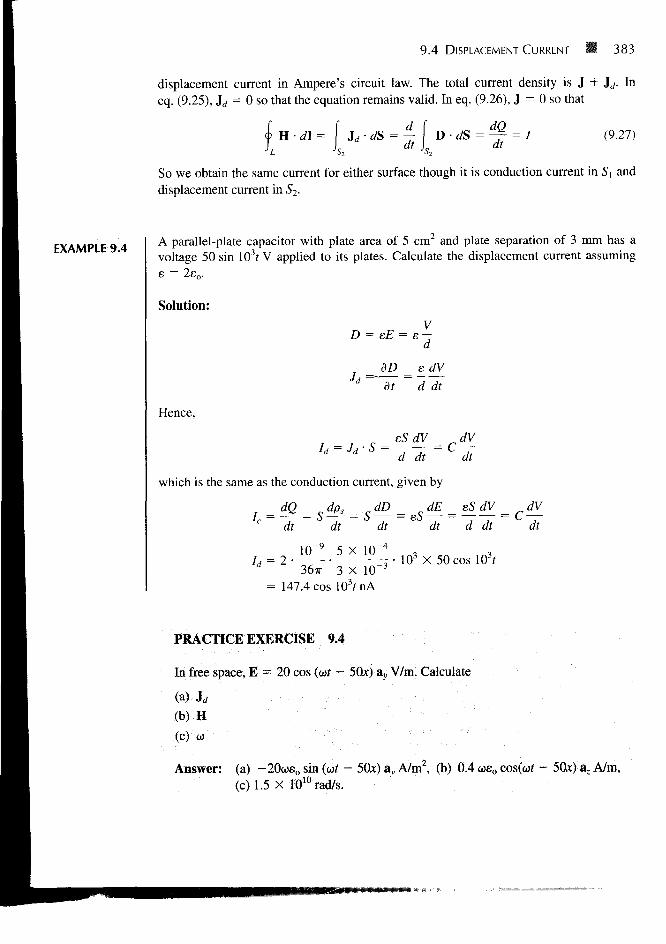
EXAMPLE 9.4A parallel-plate capacitor with plate area of 5 cm2 and plate separation of 3 mm has avoltage 50 sin 103r V applied to its plates. Calculate the displacement current assuminge = 2eo.
Solution:
D = eE = s —d
dDdt
e dv~d dt
Hence,
which is the same as the conduction current, given by
/ = 2
s
dt dt
5
dt
36TT 3 X 10"3
=
dt d dt
103 X 50 cos 10't
dV
dt
= 147.4 cos 103?nA
PRACTICE EXERCISE 9.4
In free space, E = 20 cos (at - 50xj ay V/m. Calculate
(a) h
(b) H
(c) w
Answer: (a) -20a>so sin (wt - 50J:) ay A/m2, (b) 0.4 wso cos(uit - 50x) az A/m,(c)1.5 X 1010rad/s.
384 • Maxwell's Equations
9.5 MAXWELL'S EQUATIONS IN FINAL FORMS
James Clerk Maxwell (1831-1879) is regarded as the founder of electromagnetic theory inits present form. Maxwell's celebrated work led to the discovery of electromagneticwaves.4 Through his theoretical efforts over about 5 years (when he was between 35 and40), Maxwell published the first unified theory of electricity and magnetism. The theorycomprised all previously known results, both experimental and theoretical, on electricityand magnetism. It further introduced displacement current and predicted the existence ofelectromagnetic waves. Maxwell's equations were not fully accepted by many scientistsuntil they were later confirmed by Heinrich Rudolf Hertz (1857-1894), a German physicsprofessor. Hertz was successful in generating and detecting radio waves.
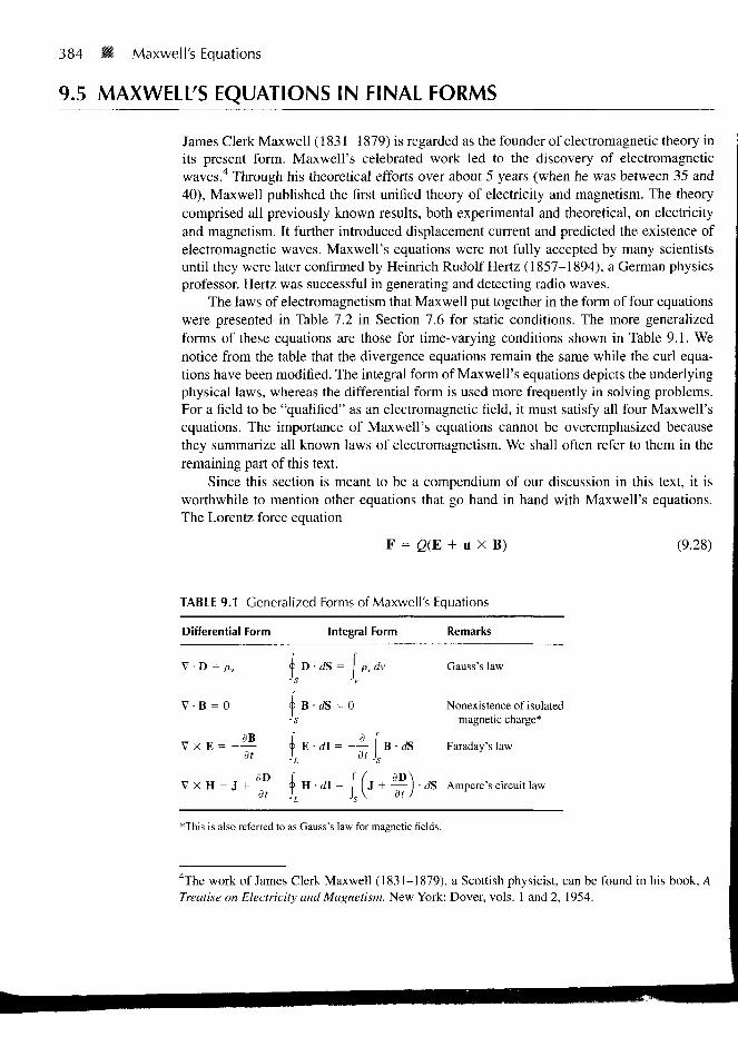
The laws of electromagnetism that Maxwell put together in the form of four equationswere presented in Table 7.2 in Section 7.6 for static conditions. The more generalizedforms of these equations are those for time-varying conditions shown in Table 9.1. Wenotice from the table that the divergence equations remain the same while the curl equa-tions have been modified. The integral form of Maxwell's equations depicts the underlyingphysical laws, whereas the differential form is used more frequently in solving problems.For a field to be "qualified" as an electromagnetic field, it must satisfy all four Maxwell'sequations. The importance of Maxwell's equations cannot be overemphasized becausethey summarize all known laws of electromagnetism. We shall often refer to them in theremaining part of this text.
Since this section is meant to be a compendium of our discussion in this text, it isworthwhile to mention other equations that go hand in hand with Maxwell's equations.The Lorentz force equation
+ u X B) (9.28)
TABLE 9.1 Generalized Forms of Maxwell's Equations
Differential
V • D = pv
V - B = O
V X E = -
V X H = J
Form
3B
dt
3D
at
1 D's
9 B
I,*<P H'L
Integral
• dS = j p,
rfS = 0
dt
Form
,rfv
B-rfS
Remarks
Gauss's law
Nonexistence of isolatedmagnetic charge*
Faraday's law
• dS Ampere's circuit law
*This is also referred to as Gauss's law for magnetic fields.
4The work of James Clerk Maxwell (1831-1879), a Scottish physicist, can be found in his book, ATreatise on Electricity and Magnetism. New York: Dover, vols. 1 and 2, 1954.
9.5 MAXWELL'S EQUATIONS IN FINAL FORMS M 385
is associated with Maxwell's equations. Also the equation of continuity
V • J = - — (9.29)dt
is implicit in Maxwell's equations. The concepts of linearity, isotropy, and homogeneity ofa material medium still apply for time-varying fields; in a linear, homogeneous, andisotropic medium characterized by a, e, and fi, the constitutive relations
D = eE = eoE + P
B = ixH = /no(H + M)
J = CTE + pvu
hold for time-varying fields. Consequently, the boundary conditions
Eu = E2t or (Ej - E2) X anl2 = 0
# u ~ H2t = K or (H, - H2) X anl2 = K
Din - D2n = p, or (D, - D2) • an l2 = p,
Bm - B2n = 0 or (B2 - B,) • aBl2 = 0
(9.30a)
(9.30b)
(9.30c)
(9.31a)
(9.31b)
(9.31c)
(9.31d)
remain valid for time-varying fields. However, for a perfect conductor (a — °°) in a time-varying field,
and hence,
E = 0, H = 0, J = 0
BB = 0, E, = 0
(9.32)
(9.33)
For a perfect dielectric (a — 0), eq. (9.31) holds except that K = 0. Though eqs. (9.28) to(9.33) are not Maxwell's equations, they are associated with them.
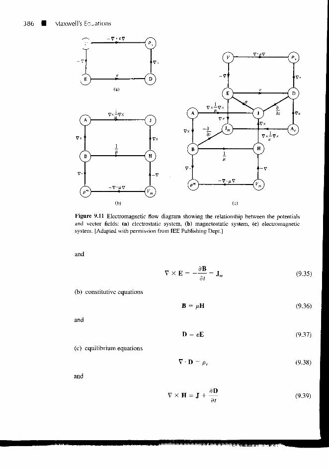
To complete this summary section, we present a structure linking the various poten-tials and vector fields of the electric and magnetic fields in Figure 9.11. This electromag-netic flow diagram helps with the visualization of the basic relationships between fieldquantities. It also shows that it is usually possible to find alternative formulations, for agiven problem, in a relatively simple manner. It should be noted that in Figures 9.10(b) and(c), we introduce pm as the free magnetic density (similar to pv), which is, of course, zero,Ae as the magnetic current density (analogous to J). Using terms from stress analysis, theprincipal relationships are typified as:
(a) compatibility equations
V • B = pm = 0 (9.34)
386 • Maxwell's Eolations
^ -v«v
(a)
Vx—Vx 0Vx ' Vx
V-'
(b) (c)
Figure 9.11 Electromagnetic flow diagram showing the relationship between the potentialsand vector fields: (a) electrostatic system, (b) magnetostatic system, (c) electromagneticsystem. [Adapted with permission from IEE Publishing Dept.]
and
(b) constitutive equations
and
(c) equilibrium equations
and
B = ,uH
D = eE
V • D = Pv
dt
9.6 TIME-VARYING POTENTIALS 387
9.6 TIME-VARYING POTENTIALS
For static EM fields, we obtained the electric scalar potential as
pvdv
and the magnetic vector potential as
V =
A =
AireR
fiJ dv
4wR
(9.40)
(9.41)
We would like to examine what happens to these potentials when the fields are timevarying. Recall that A was defined from the fact that V • B = 0, which still holds for time-varying fields. Hence the relation
B = V X A (9.42)
holds for time-varying situations. Combining Faraday's law in eq. (9.8) with eq. (9.42) gives
V X E = (V X A) (9.43a)
or
V X | E + - | =dt
(9.43b)
Since the curl of the gradient of a scalar field is identically zero (see Practice Exercise3.10), the solution to eq. (9.43b) is
dt
or
dt
(9.44)
(9.45)
From eqs. (9.42) and (9.45), we can determine the vector fields B and E provided that thepotentials A and V are known. However, we still need to find some expressions for A andV similar to those in eqs. (9.40) and (9.41) that are suitable for time-varying fields.
From Table 9.1 or eq. (9.38) we know that V • D = pv is valid for time-varying condi-tions. By taking the divergence of eq. (9.45) and making use of eqs. (9.37) and (9.38), weobtain
V - E = — = - V 2 V - — ( V - A )e dt
388 Maxwell's Equations
or
VV + ( V A )dt e
Taking the curl of eq. (9.42) and incorporating eqs. (9.23) and (9.45) results in
VX V X A = uj + e/n — ( -VVdt V dt
dV
(9.46)
where D = sE and B = fiH have been assumed. By applying the vector identity
V X V X A = V(V • A) - V2A
to eq. (9.47),
V2A - V(V • A) = -f + \dt
d2A—r-dt2
(9.47)
(9.48)
(9.49)
A vector field is uniquely defined when its curl and divergence are specified. The curl of Ahas been specified by eq. (9.42); for reasons that will be obvious shortly, we may choosethe divergence of A as
V • A = -JdV_
dt(9.50)
This choice relates A and V and it is called the Lorentz condition for potentials. We had thisin mind when we chose V • A = 0 for magnetostatic fields in eq. (7.59). By imposing theLorentz condition of eq. (9.50), eqs. (9.46) and (9.49), respectively, become
(9.51)
and
2
V2A JUS
d2V
dt2
a2 A
dt2
Pve
y
/xj (9.52)
which are wave equations to be discussed in the next chapter. The reason for choosing theLorentz condition becomes obvious as we examine eqs. (9.51) and (9.52). It uncoupleseqs. (9.46) and (9.49) and also produces a symmetry between eqs. (9.51) and (9.52). It canbe shown that the Lorentz condition can be obtained from the continuity equation; there-fore, our choice of eq. (9.50) is not arbitrary. Notice that eqs. (6.4) and (7.60) are specialstatic cases of eqs. (9.51) and (9.52), respectively. In other words, potentials V and Asatisfy Poisson's equations for time-varying conditions. Just as eqs. (9.40) and (9.41) are
9.7 TIME-HARMONIC FIELDS 389
the solutions, or the integral forms of eqs. (6.4) and (7.60), it can be shown that the solu-tions5 to eqs. (9.51) and (9.52) are
V =[P.] dv
A-KSR
and
A =A-KR
(9.53)
(9.54)
The term [pv] (or [J]) means that the time t in pv(x, y, z, t) [or J(x, y, z, t)] is replaced by theretarded time t' given by
(9.55)
where R = |r — r ' | is the distance between the source point r ' and the observation point rand
1u = (9.56)
/xe
is the velocity of wave propagation. In free space, u = c — 3 X 1 0 m/s is the speed oflight in a vacuum. Potentials V and A in eqs. (9.53) and (9.54) are, respectively, called theretarded electric scalar potential and the retarded magnetic vector potential. Given pv andJ, V and A can be determined using eqs. (9.53) and (9.54); from V and A, E and B can bedetermined using eqs. (9.45) and (9.42), respectively.
9.7 TIME-HARMONIC FIELDS
So far, our time dependence of EM fields has been arbitrary. To be specific, we shallassume that the fields are time harmonic.
A time-harmonic field is one thai varies periodically or sinusoidally wiih time.
Not only is sinusoidal analysis of practical value, it can be extended to most waveforms byFourier transform techniques. Sinusoids are easily expressed in phasors, which are moreconvenient to work with. Before applying phasors to EM fields, it is worthwhile to have abrief review of the concept of phasor.
Aphasor z is a complex number that can be written as
z = x + jy = r (9.57)
1983, pp. 291-292.
390 Maxwell's Equations
or„ = r „)<$> == r e = r (cos <j> + j sin - (9.58)
where j = V — 1, x is the real part of z, y is the imaginary part of z, r is the magnitude ofz, given by
r —
and cj> is the phase of z, given by
= tan'1 l
(9.59)
(9.60)
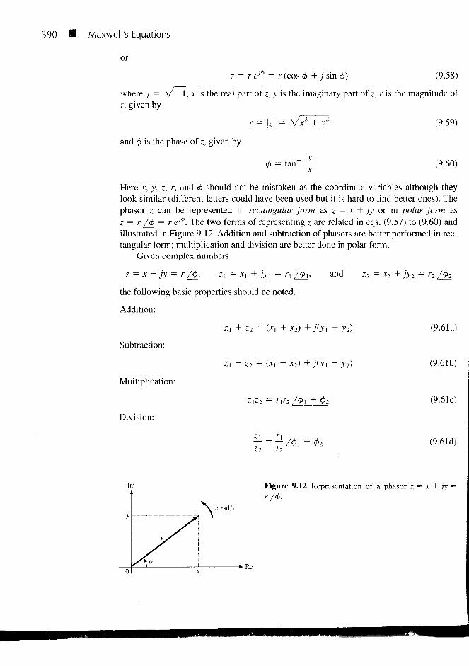
Here x, y, z, r, and 0 should not be mistaken as the coordinate variables although theylook similar (different letters could have been used but it is hard to find better ones). Thephasor z can be represented in rectangular form as z = x + jy or in polar form asz = r [§_ = r e'^. The two forms of representing z are related in eqs. (9.57) to (9.60) andillustrated in Figure 9.12. Addition and subtraction of phasors are better performed in rec-tangular form; multiplication and division are better done in polar form.
Given complex numbers
z = x + jy = r[$_, z, = x, + jy, = r, /
the following basic properties should be noted.
Addition:
Subtraction:
Multiplication:
Division:
x2)
x2)
and z2 = x2 + jy2 = r2 /<j>2
y2) (9.61a)
- y2) (9.61b)
(9.61c)
(9.61d)
lm
co rad/s
Figure 9.12 Representation of a phasor z = x + jyr /<t>.
•Re
9.7 TIME-HARMONIC FIELDS H 391
Square Root:
Complex Conjugate:
Z = Vr
Z* = x — jy = r/—<j> == re
Other properties of complex numbers can be found in Appendix A.2.To introduce the time element, we let
(9.61e)
(9.61f)
(9.62)
where 6 may be a function of time or space coordinates or a constant. The real (Re) andimaginary (Im) parts of
= rejeeJo"
are, respectively, given by
and
Re (rej<t>) = r cos (ut + 0)
Im {rei4>) = r sin (art + 0)
(9.63)
(9.64a)
(9.64b)
Thus a sinusoidal current 7(0 = 7O cos(wt + 0), for example, equals the real part ofIoe
jeeM. The current 7'(0 = h sin(co? + 0), which is the imaginary part of Ioe]ee]01t, can
also be represented as the real part of Ioejeeju"e~j90° because sin a = cos(a - 90°).
However, in performing our mathematical operations, we must be consistent in our use ofeither the real part or the imaginary part of a quantity but not both at the same time.
The complex term Ioeje, which results from dropping the time factor ejo" in 7(0, is
called the phasor current, denoted by 7 ; that is,
]s = io(,J» = 70 / 0 (9.65)
where the subscript s denotes the phasor form of 7(0- Thus 7(0 = 70 cos(cof + 0), the in-stantaneous form, can be expressed as
= Re (9.66)
In general, a phasor could be scalar or vector. If a vector A(*, y, z, t) is a time-harmonicfield, the phasor form of A is As(x, y, z); the two quantities are related as
A = Re (XseJo")
For example, if A = Ao cos (ut — j3x) ay, we can write A as
A = Re (Aoe-j0x a / u ' )
Comparing this with eq. (9.67) indicates that the phasor form of A is
(9.67)
(9.68)
**-s AQ€ (9.69)
392 M Maxwell's Equations
Notice from eq. (9.67) that
(9.70)= Re (/«A/M()
showing that taking the time derivative of the instantaneous quantity is equivalent to mul-tiplying its phasor form byyco. That is,
<3A
Similarly,
(9.71)
(9.72)
Note that the real part is chosen in eq. (9.67) as in circuit analysis; the imaginary partcould equally have been chosen. Also notice the basic difference between the instanta-neous form A(JC, y, z, t) and its phasor form As(x, y, z); the former is time dependent andreal whereas the latter is time invariant and generally complex. It is easier to work with Aand obtain A from As whenever necessary using eq. (9.67).
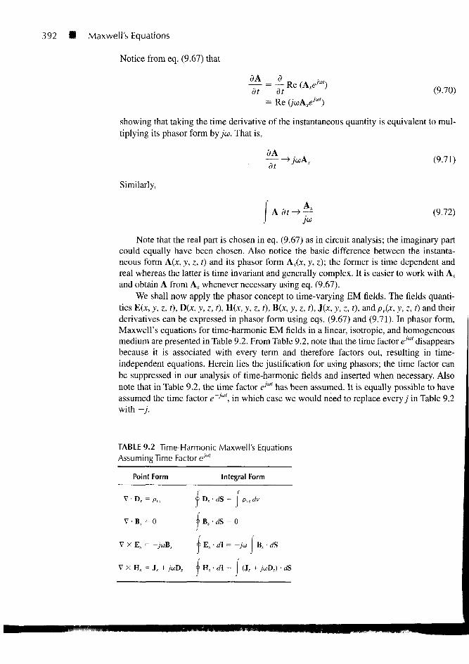
We shall now apply the phasor concept to time-varying EM fields. The fields quanti-ties E(x, y, z, t), D(x, y, z, t), H(x, y, z, t), B(x, y, z, t), J(x, y, z, t), and pv(x, y, z, i) and theirderivatives can be expressed in phasor form using eqs. (9.67) and (9.71). In phasor form,Maxwell's equations for time-harmonic EM fields in a linear, isotropic, and homogeneousmedium are presented in Table 9.2. From Table 9.2, note that the time factor eJa" disappearsbecause it is associated with every term and therefore factors out, resulting in time-independent equations. Herein lies the justification for using phasors; the time factor canbe suppressed in our analysis of time-harmonic fields and inserted when necessary. Alsonote that in Table 9.2, the time factor e'01' has been assumed. It is equally possible to haveassumed the time factor e~ja", in which case we would need to replace every y in Table 9.2with —j.
TABLE 9.2 Time-Harmonic Maxwell's EquationsAssuming Time Factor e'""
Point Form Integral Form
Dv • dS = I pvs dv
B5 • dS = 0
V • D v = />„.,
V • B.v = 0
V X E s = -joiB, <k E s • d\ = -ju> I Bs • dS
V X H, = Js + juDs §Hs-dl= [ (J s + joiDs) • dS
9.7 TIME-HARMONIC FIELDS 393
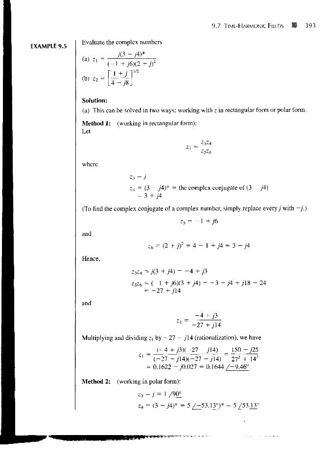
EXAMPLE 9.5Evaluate the complex numbers
7(3 - ;4)*(a) z, =
( -111/2
Solution:
(a) This can be solved in two ways: working with z in rectangular form or polar form.
Method 1: (working in rectangular form):Let
_ Z3Z4
where
£3 =j
z,4 = (3 - j4)* = the complex conjugate of (3 - j4)= 3 + ;4
(To find the complex conjugate of a complex number, simply replace every) with —j.)
z5 = - 1 +76
and
Hence,
z3z4 = j4) = - 4
and
= (-1 + j6)(3 + ;4) = - 3 - ;4= -27+ ;14
- 4 + ;3
- 24
*"' - 2 7 + 7 I 4
Multiplying and dividing z\ by -27 - j\4 (rationalization), we have
(-4 + j3)(-27 - yi4) _ 150 -J25Zl ~ (-27 +yl4)(-27 -j'14) 272 + 142
= 0.1622 -;0.027 = 0.1644 / - 9.46°
Method 2: (working in polar form):
z3=j= 1/90°
z4 = (3 - j4)* = 5 /-53.130)* = 5 /53.13°
394 • Maxwell's Equations
Hence,
as obtained before,
(b) Let
where
and
Hence
z5 = ("I +j6) = V37 /99.46°
zb = (2 + jf = (V5 /26.56°)2 = 5 /53.130
(1 /90°)(5 /53.130)
and
(V37 /99.46°)(5 /53.130)
1 /90° - 99.46° = 0.1644 /-9.46°V37
= 0.1622 - 70.027
1/2
Zs
Z7=l+j= V2/45°
= 4 -78 = 4V5/-63.4O
V2 /45° V2
4V5/-63.40 4V50.1581 7108.4°
/45° 63.4°
z2 = V0.1581 /108.472= 0.3976 754.2°
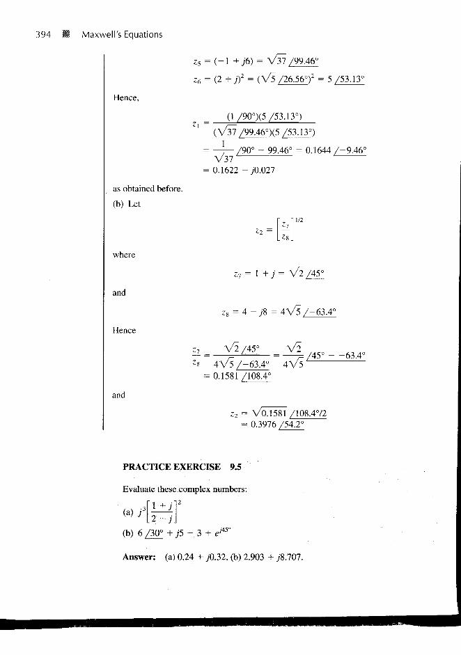
PRACTICE EXERCISE 9.5
Evaluate these complex numbers:
(b) 6 /W_ + ;5 - 3 + ejn
Answer: (a) 0.24 + j0.32, (b) 2.903 + J8.707.
9.7 TIME-HARMONIC FIELDS • 395
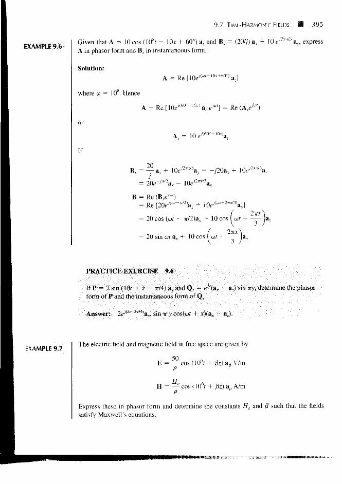
EXAMPLE 9.6Given that A = 10 cos (108? - 10* + 60°) az and Bs = (20//) a, + 10 ej2"B ay, expressA in phasor form and B^ in instantaneous form.
Solution:
where u = 10 . Hence
A = Re[10e'M~1 0 A H
If
A = Re [\0eJ(bU ~lw az e*"] = Re ( A , O
A, = ]0ej
90e / 2" / 3a = - jB, = — a , + 10e / 2" / 3ay = - j20a v
2 / 2 / 3
B = Re (B.e-"0')= Re [20ej(w("7r/2)ax + lO^'(w'+2TJ[/3)a),]
/ 2TT*\= 20 cos (art - 7r/2)a.v + 10 cos I wf + — - lav
= 20 sin o)t ax + 10 cos —r— jav
PRACTICE EXERCISE 9.6
If P = 2 sin (]Qt + x - TT/4) av and Qs = ej*(ax - a.) sin Try, determine the phasorform of P and the instantaneous form of Qv.
Answer: 2eju" Jx/4)av, sin x y cos(wf + jc)(a,. - ar).
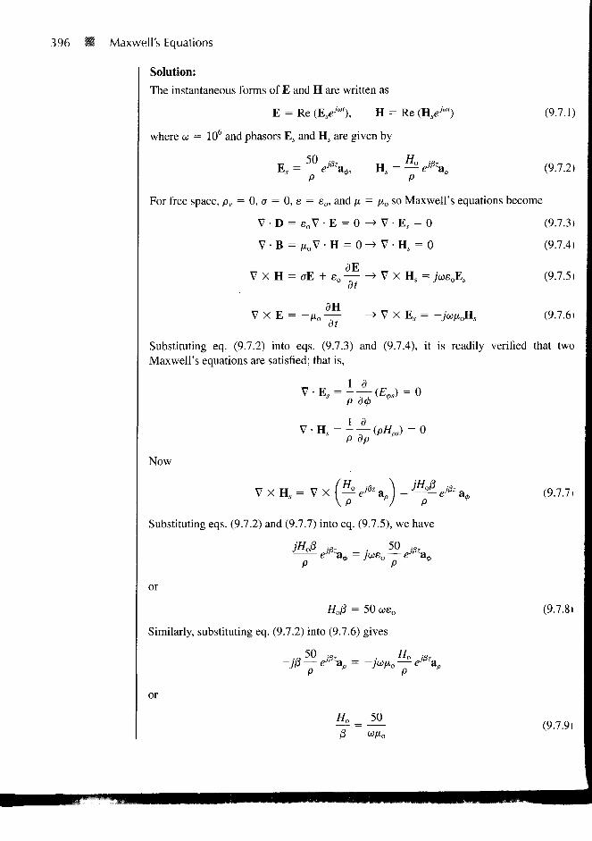
EXAMPLE 9.7The electric field and magnetic field in free space are given by
E = — cos (l06f + /3z) a* V/mP
H = —^ cos (l06f + |3z) a0 A/m
Express these in phasor form and determine the constants Ho and /3 such that the fieldssatisfy Maxwell's equations.
396 • Maxwell's Equations
Solution:
The instantaneous forms of E and H are written as
E = Re (EseJal), H = Re (Hse
J"')
where co = 106 and phasors Es and Hs are given by
50 HE = —' e^a H = — e^za
p *' p "For free space, pv = 0, a = 0, e = eo, and ft = fio so Maxwell's equations become
V-B = |ioV-H = 0-> V-Ha: = 0
dE
dt> V X H S = j
•iii
V X E = -fio —
(9.7.1)
(9.7.2)
(9.7.3)
(9.7.4)
(9.7.5)
(9.7.6)
Substituting eq. (9.7.2) into eqs. (9.7.3) and (9.7.4), it is readily verified that twoMaxwell's equations are satisfied; that is,
Now
V X Hs = V XP V P
Substituting eqs. (9.7.2) and (9.7.7) into eq. (9.7.5), we have
JHOI3 mz . 50 M,
(9.7.7i
or
//o/3 = 50 a)eo
Similarly, substituting eq. (9.7.2) into (9.7.6) gives
P
or
(9.7.8)
(9.7.9)
9.7 TIME-HARMONIC FIELDS 397
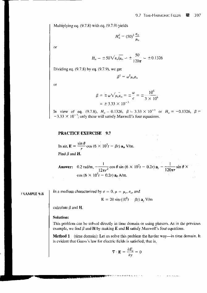
Multiplying eq. (9.7.8) with eq. (9.7.9) yields
or
Mo
50Ho = ±50V sJno = ± 7 ^ " = ± 0 - 1 3 2 6
Dividing eq. (9.7.8) by eq. (9.7.9), we get
I32 = o;2/x0e0
or
0 = ± aVp,
= ±3.33 X 10
10"
3 X 10s
- 3
In view of eq. (9.7.8), Ho = 0.1326, & = 3.33 X 10~3 or Ho = -0.1326, j3 =— 3.33 X 10~3; only these will satisfy Maxwell's four equations.
PRACTICE EXERCISE 9.7
In air, E = ^— cos (6 X 10⁷r - /3r) a* V/m.r
Find j3 and H.
Answer: 0.2 rad/m, r cos 6 sin (6 X 10⁷? - 0.2r) ar — sin S Xllzr2 1207rr
cos (6 X 10⁷f - 0.2r) % A/m.
EXAMPLE 9.8In a medium characterized by a = 0, \x = /xo, eo, and
E = 20 sin (108f - j3z) a7 V/m
calculate /8 and H.
Solution:
This problem can be solved directly in time domain or using phasors. As in the previousexample, we find 13 and H by making E and H satisfy Maxwell's four equations.
Method 1 (time domain): Let us solve this problem the harder way—in time domain. Itis evident that Gauss's law for electric fields is satisfied; that is,
dy
398 • Maxwell's Equations
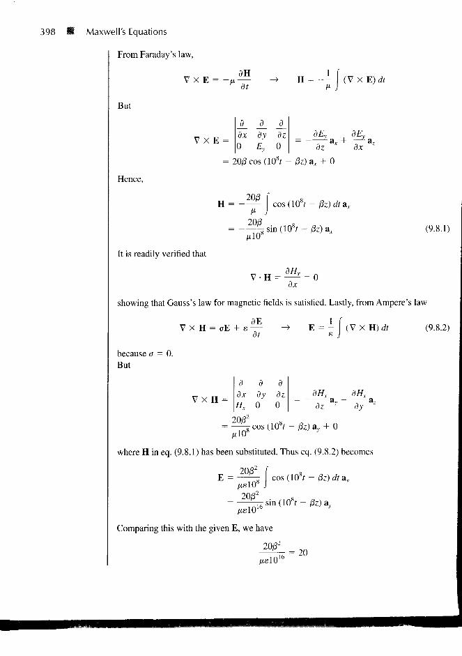
From Faraday's law,
V X E = - /
But
V X E =
dHdt
A A Adx dy dz0 Ey 0
H = - - I (V X E)dt
dEy dEy
dz dx
Hence,
= 20/3 cos (108f - (3z) ax + 0
H = cos (108r - pz) dtax
^ s i - I3z)ax (9.8.1)
It is readily verified that
dx
showing that Gauss's law for magnetic fields is satisfied. Lastly, from Ampere's law
V X H = CTE + £1
E = - | (V X H) (9.8.2)
because a = 0.But
V X H =A A Adx dy dzHr 0 0
dHx dHx
cos(108? - $z)ay + 0
where H in eq. (9.8.1) has been substituted. Thus eq. (9.8.2) becomes
20/S2
E = cos(10 8r- (3z)dtay
2O/32
•sin(108f -
Comparing this with the given E, we have
= 20
9.7 TIME-HARMONIC FIELDS • 399
or
= ± 108Vtis = ± 10SVIXO • 4eo = ±108(2) 108(2)
3 X 10B
From eq. (9.8.1),
or
1 / 2z\H = ± — sin 108?±— axA/m
3TT V 3/
Method 2 (using phasors):
E = Im ( £ y ) -> E, = av
where co =Again
10°.
V X E, =
dy
• -> " H, =V X Es
or
20/3 fr
Notice that V • H, = 0 is satisfied.
V X Hs = ji E, =V X H,
jus
Substituting H^ in eq. (9.8.4) into eq. (9.8.5) gives
2co /xe
Comparing this with the given Es in eq. (9.8.3), we have
^co /xe
(9.8.3)
(9.8.4)
(9.8.5)
400 Maxwell's Equations
or
as obtained before. From eq. (9.8.4),
„ ^ 2 0 ( 2 / 3 ) ^
10 8 (4T X 10 ') 3TT
H = Im (H/" 1 )
= ± — sin (108f ± Qz) ax A/m3TT
as obtained before. It should be noticed that working with phasors provides a considerablesimplification compared with working directly in time domain. Also, notice that we haveused
A = Im (Asejat)
because the given E is in sine form and not cosine. We could have used
A = Re (Asejo")
in which case sine is expressed in terms of cosine and eq. (9.8.3) would be
E = 20 cos (108? - & - 90°) av = Re (EseM)
or
and we follow the same procedure.
PRACTICE EXERCISE 9.8
A medium is characterized by a = 0, n = 2/*,, and s = 5eo. If H = 2cos {(jit — 3y) a_, A/m, calculate us and E.
Answer: 2.846 X l(f rad/s, -476.8 cos (2.846 X 10⁸f - 3v) a, V/m.
SUMMARY 1. In this chapter, we have introduced two fundamental concepts: electromotive force(emf), based on Faraday's experiments, and displacement current, which resulted fromMaxwell's hypothesis. These concepts call for modifications in Maxwell's curl equa-tions obtained for static EM fields to accommodate the time dependence of the fields.
2. Faraday's law states that the induced emf is given by (N = 1)
dt
REVIEW QUESTIONS U 401
For transformer emf, Vemf = — ,
and for motional emf, Vemf = I (u X B) • d\.
3. The displacement current
h = ( h • dS
dDwhere id = (displacement current density), is a modification to Ampere's circuit
dt
law. This modification attributed to Maxwell predicted electromagnetic waves severalyears before it was verified experimentally by Hertz.
4. In differential form, Maxwell's equations for dynamic fields are:
V • D = Pv
V-B = 0
dt
V X H J +
dt
Each differential equation has its integral counterpart (see Tables 9.1 and 9.2) that canbe derived from the differential form using Stokes's or divergence theorem. Any EMfield must satisfy the four Maxwell's equations simultaneously.
5. Time-varying electric scalar potential V(x, y, z, t) and magnetic vector potentialA(JC, y, z, t) are shown to satisfy wave equations if Lorentz's condition is assumed.
6. Time-harmonic fields are those that vary sinusoidally with time. They are easily ex-pressed in phasors, which are more convenient to work with. Using the cosine refer-ence, the instantaneous vector quantity A(JC, y, z, t) is related to its phasor formAs(x, y, z) according to
A(x, y, z, t) = Re [AX*, y, z) eM]
9.1 The flux through each turn of a 100-turn coil is (t3 — 2t) mWb^ where t is in seconds.The induced emf at t = 2 s is
(a) IV
(b) - 1 V
(c) 4mV
(d) 0.4 V(e) -0.4 V
402 B Maxwell's Equations
, Increasing B
(a)
Decreasing BFigure 9.13 For Review Question 9.2.
(b)
• Decreasing B Increasing B
(d)
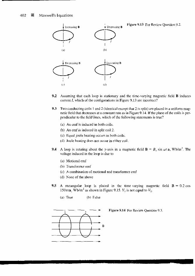
9.2 Assuming that each loop is stationary and the time-varying magnetic field B inducescurrent /, which of the configurations in Figure 9.13 are incorrect?
9.3 Two conducting coils 1 and 2 (identical except that 2 is split) are placed in a uniform mag-netic field that decreases at a constant rate as in Figure 9.14. If the plane of the coils is per-pendicular to the field lines, which of the following statements is true?
(a) An emf is induced in both coils.
(b) An emf is induced in split coil 2.
(c) Equal joule heating occurs in both coils.
(d) Joule heating does not occur in either coil.
9.4 A loop is rotating about the y-axis in a magnetic field B = Ba sin wt ax Wb/m2. Thevoltage induced in the loop is due to
(a) Motional emf
(b) Transformer emf
(c) A combination of motional and transformer emf
(d) None of the above
9.5 A rectangular loop is placed in the time-varying magnetic field B = 0.2 cos150irfaz Wb/m as shown in Figure 9.15. Vx is not equal to V2.
(a) True (b) False
Figure 9.14 For Review Question 9.3.
REVIEW QUESTIONS • 403
©
©
©
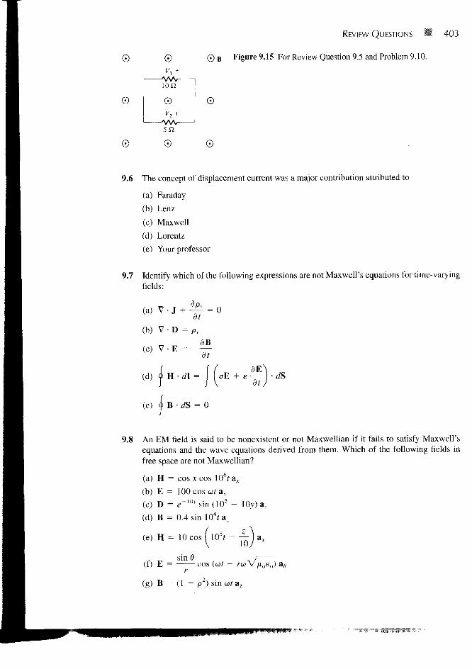
0 B Figure 9.15 For Review Question 9.5 and Problem 9.10.
9.6 The concept of displacement current was a major contribution attributed to
(a) Faraday
(b) Lenz
(c) Maxwell
(d) Lorentz
(e) Your professor
9.7 Identify which of the following expressions are not Maxwell's equations for time-varyingfields:
(a)
(b) V • D = Pv
(d) 4> H • d\ =
(e) i B • dS = 0
+ e ) • dSdt J
9.8 An EM field is said to be nonexistent or not Maxwellian if it fails to satisfy Maxwell'sequations and the wave equations derived from them. Which of the following fields infree space are not Maxwellian?
(a) H = cos x cos 106fav
(b) E = 100 cos cot ax
(c) D = e"10> 'sin(105 - lOy) az
(d) B = 0.4 sin 104fa.
(e) H = 10 cos ( 103/ - — | a r
sinfl(f) E = cos i
V/ioeo) i
(g) B = (1 - p ) sin u>faz
404 Maxwell's Equations
9.9 Which of the following statements is not true of a phasor?
(a) It may be a scalar or a vector.
(b) It is a time-dependent quantity.(c) A phasor Vs may be represented as Vo / 0 or Voe
je where Vo = | Vs
(d) It is a complex quantity.
9.10 If Ej = 10 ej4x ay, which of these is not a correct representation of E?
(a) Re (Esejut)
(b) Re (Ese-j"')
(c) Im (E.^"")(d) 10 cos (wf + jAx) ay
(e) 10 sin (ut + Ax) ay
Answers: 9.1b, 9.2b, d, 9.3a, 9.4c, 9.5a, 9.6c, 9.7a, b, d, g, 9.8b, 9.9a,c, 9.10d.
PRORI FMS ' '* ^ conducting circular loop of radius 20 cm lies in the z = 0 plane in a magnetic fieldB = 10 cos 377? az mWb/m2. Calculate the induced voltage in the loop.
9.2 A rod of length € rotates about the z-axis with an angular velocity w. If B = Boaz, calcu-late the voltage induced on the conductor.
9.3 A 30-cm by 40-cm rectangular loop rotates at 130 rad/s in a magnetic field 0.06 Wb/m2
normal to the axis of rotation. If the loop has 50 turns, determine the induced voltage inthe loop.
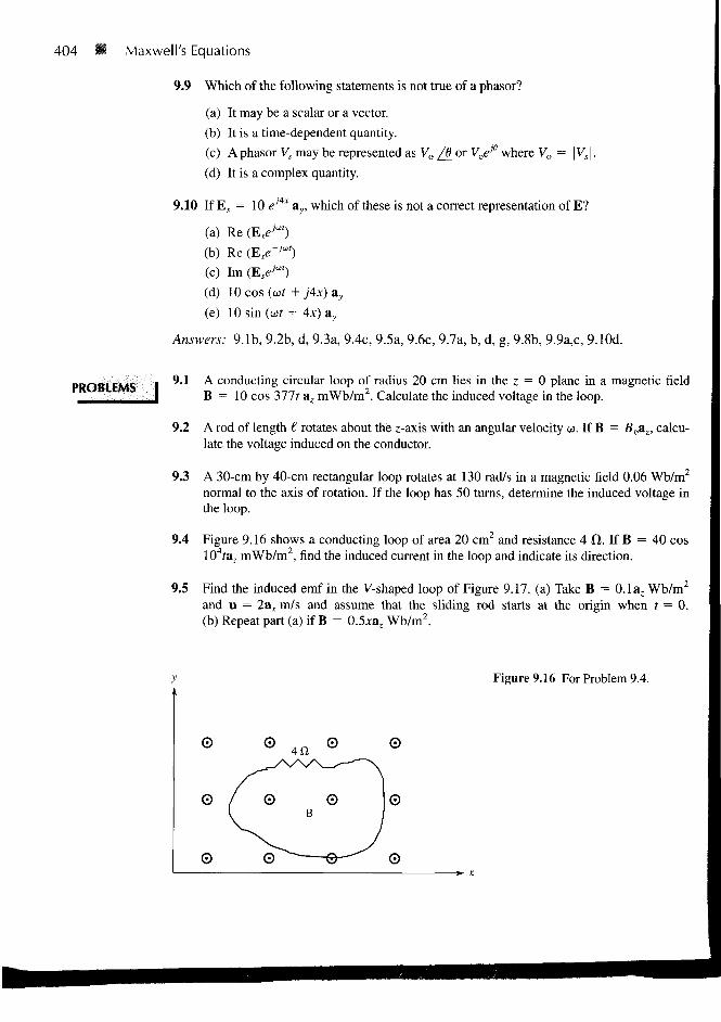
9.4 Figure 9.16 shows a conducting loop of area 20 cm2 and resistance 4 fl. If B = 40 cos104faz mWb/m2, find the induced current in the loop and indicate its direction.
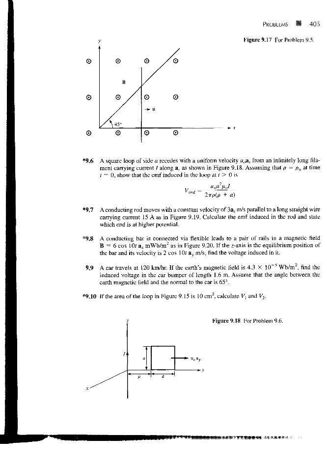
9.5 Find the induced emf in the V-shaped loop of Figure 9.17. (a) Take B = 0.1a, Wb/m2
and u = 2ax m/s and assume that the sliding rod starts at the origin when t = 0.(b) Repeat part (a) if B = 0.5xaz Wb/m2.
Figure 9.16 For Problem 9.4.
©
© /\
©
©
©
\ .0
4f i
B
^ -
©
— \1
©
1
©
©
©
©
0
©
PROBLEMS • 405
Figure 9.17 For Problem 9.5.
©
B
0 /
/V©
©
0
-»- u
©
0
©
*9.6 A square loop of side a recedes with a uniform velocity «oav from an infinitely long fila-ment carrying current / along az as shown in Figure 9.18. Assuming that p = po at timet = 0, show that the emf induced in the loop at t > 0 is
Vrmf = uoa2vp{p + a)
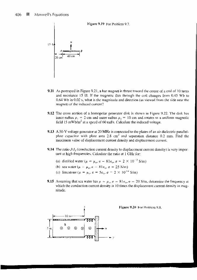
*9.7 A conducting rod moves with a constant velocity of 3az m/s parallel to a long straight wirecarrying current 15 A as in Figure 9.19. Calculate the emf induced in the rod and statewhich end is at higher potential.
*9.8 A conducting bar is connected via flexible leads to a pair of rails in a magnetic fieldB = 6 cos lOf ax mWb/m2 as in Figure 9.20. If the z-axis is the equilibrium position ofthe bar and its velocity is 2 cos lOf ay m/s, find the voltage induced in it.
9.9 A car travels at 120 km/hr. If the earth's magnetic field is 4.3 X 10"5 Wb/m2, find theinduced voltage in the car bumper of length 1.6 m. Assume that the angle between theearth magnetic field and the normal to the car is 65°.
*9.10 If the area of the loop in Figure 9.15 is 10 cm2, calculate Vx and V2.
Figure 9.18 For Problem 9.6.
406 Maxwell's Equations
15 A
A
20 cm
u
t40 cm
Figure 9.19 For Problem 9.7.
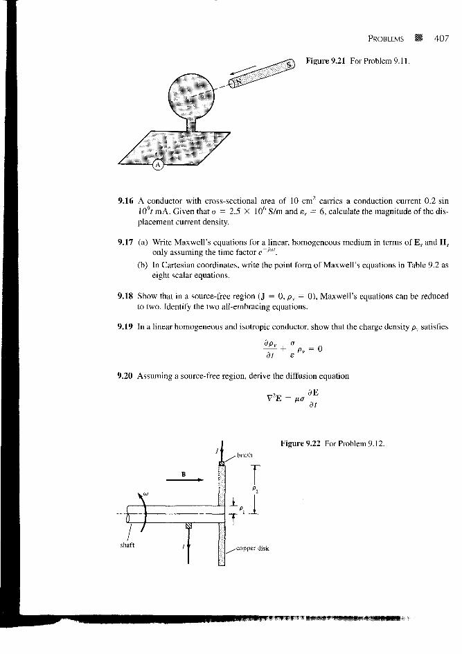
9.11 As portrayed in Figure 9.21, a bar magnet is thrust toward the center of a coil of 10 turnsand resistance 15 fl. If the magnetic flux through the coil changes from 0.45 Wb to0.64 Wb in 0.02 s, what is the magnitude and direction (as viewed from the side near themagnet) of the induced current?
9.12 The cross section of a homopolar generator disk is shown in Figure 9.22. The disk hasinner radius p] = 2 cm and outer radius p2 = 10 cm and rotates in a uniform magneticfield 15 mWb/m2 at a speed of 60 rad/s. Calculate the induced voltage.
9.13 A 50-V voltage generator at 20 MHz is connected to the plates of an air dielectric parallel-plate capacitor with plate area 2.8 cm2 and separation distance 0.2 mm. Find themaximum value of displacement current density and displacement current.
9.14 The ratio JIJd (conduction current density to displacement current density) is very impor-tant at high frequencies. Calculate the ratio at 1 GHz for:
(a) distilled water (p = ,uo, e = 81e0, a = 2 X 10~3 S/m)
(b) sea water (p, = no, e = 81eo, a = 25 S/m)
(c) limestone {p. = ixo, e = 5eo, j = 2 X 10~4 S/m)
9.15 Assuming that sea water has fi = fxa, e = 81e0, a = 20 S/m, determine the frequency atwhich the conduction current density is 10 times the displacement current density in mag-nitude.
Figure 9.20 For Problem 9.8.
PROBLEMS
Figure 9.21 For Problem 9.11.
407
9.16 A conductor with cross-sectional area of 10 cm carries a conduction current 0.2 sinl09t mA. Given that a = 2.5 X 10⁶ S/m and e r = 6, calculate the magnitude of the dis-placement current density.
9.17 (a) Write Maxwell's equations for a linear, homogeneous medium in terms of Es and YLS
only assuming the time factor e~Ju".
(b) In Cartesian coordinates, write the point form of Maxwell's equations in Table 9.2 aseight scalar equations.
9.18 Show that in a source-free region (J = 0, pv = 0), Maxwell's equations can be reducedto two. Identify the two all-embracing equations.
9.19 In a linear homogeneous and isotropic conductor, show that the charge density pv satisfies
— + -pv = 0dt e
9.20 Assuming a source-free region, derive the diffusion equation
at
shaft
brush
copper disk
Figure 9.22 For Problem 9.12.
408 'axwell's Eolations
9.21 In a certain region,
J = (2yax + xzay + z3az) sin 104r A/m
nndpvifpv(x,y,0,t) = 0.
9.22 In a charge-free region for which a = 0, e = eoer, and /* = /xo,
H = 5 c o s ( 1 0 u ? - 4y)a,A/m
find: (a) Jd and D, (b) er.
9.23 In a certain region with a = 0, /x = yuo, and e = 6.25a0, the magnetic field of an EMwave is
H = 0.6 cos I3x cos 108r a, A/m
Find /? and the corresponding E using Maxwell's equations.
*9.24 In a nonmagnetic medium,
E = 50 cos(109r - Sx)&y + 40 sin(109? - Sx)az V/m
find the dielectric constant er and the corresponding H.
9.25 Check whether the following fields are genuine EM fields, i.e., they satisfy Maxwell'sequations. Assume that the fields exist in charge-free regions.
(a) A = 40 sin(co? + 10r)a2
(b) B = — cos(cor - 2p)a6P
(c) C = f 3 p 2 cot <j>ap H a 0 j sin u>t
(d) D = — sin 8 sm(wt — 5r)aer
**9.26 Given the total electromagnetic energy
W = | (E • D + H • B) dv
show from Maxwell's equations that
dWdt = - f (EXH)-(iS- E • J dv
9.27 In free space,
H = p(sin 4>ap + 2 cos ^ a j cos 4 X 10 t A/m
find id and E.
PROBLEMS 409
9.28 An antenna radiates in free space and
12 sin 6H = cos(2ir X l(fr - 0r)ag mA/m
find the corresponding E in terms of /3.
*9.29 The electric field in air is given by E = pte~p~\ V/m; find B and J.
**9.30 In free space (pv = 0, J = 0). Show that
A = -£2_ ( c o s e a r _ s i n e ajeJ*'-"*A-wr
satisfies the wave equation in eq. (9.52). Find the corresponding V. Take c as the speed oflight in free space.
9.31 Evaluate the following complex numbers and express your answers in polar form:
(a) (4 /30° - 10/50°)1/2
1 +J2(b)
(c)
(d)
6 + 7 8 - 7(3 + j4)2
12 - jl + ( -6 +;10)*
(3.6/-200°)1 /2
9.32 Write the following time-harmonic fields as phasors:
(a) E = 4 cos(oit - 3x - 10°) ay - sin(cof + 3x + 20°) B;,
sin(b) H = cos(ut - 5r)ag
r(c) J = 6e~3x sin(ojf — 2x)ay + 10e~*cos(w? —
9.33 Express the following phasors in their instantaneous forms:
(a) A, = (4 - 3j)e-j0xay
0 » B , = ^ - * %
(c) Cs = —7 (1 + j2)e~j<t> sin 0 a 0r
9.34 Given A = 4 sin wtax + 3 cos wtay and Bs = j\0ze~jzax, express A in phase form andB, in instantaneous form.
9.35 Show that in a linear homogeneous, isotropic source-free region, both Es and Hs mustsatisfy the wave equation
, = 0
where y2 = a>2/xe and A = E,, or Hs.