Chap3b.continuous Distrib

Introduction to Statistics Mathematics

Chapter Continuous Distributions

Chapter Topics

Gamma Distribution Weibull Distribution Exponential Distribution The normal distribution The standardized normal distribution Evaluating the normality assumption

Continuous Probability Distributions

Continuous random variable Values from interval of numbers Absence of gaps

Continuous probability distribution Distribution of continuous random variable

Most important continuous probability distribution The normal distribution

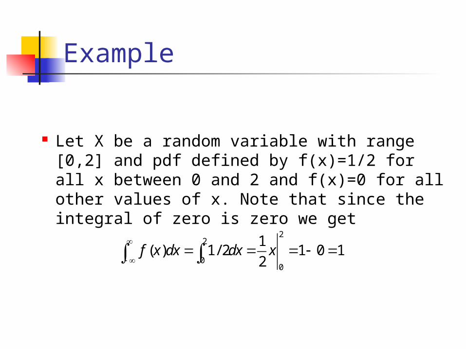
Let X be a random variable with range [0,2] and pdf defined by f(x)=1/2 for all x between 0 and 2 and f(x)=0 for all other values of x. Note that since the integral of zero is zero we get

22

00

1( ) 1/ 2 1 0 1

2f x dx dx x

Example

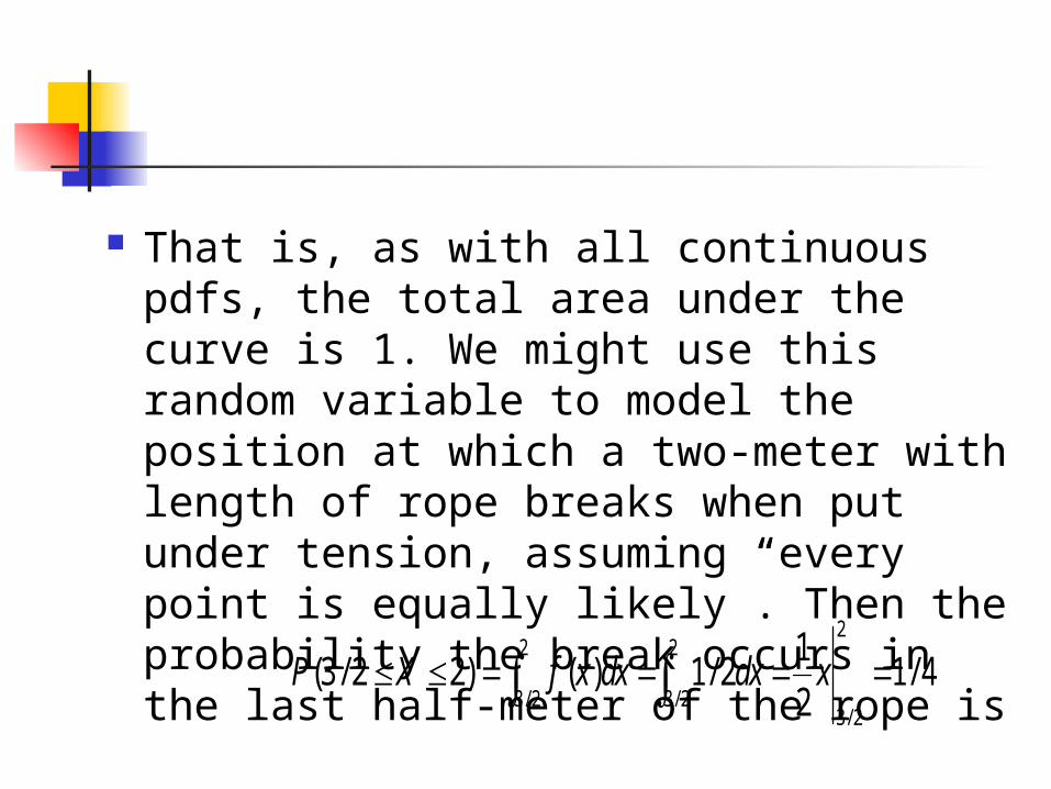
That is, as with all continuous pdfs, the total area under the curve is 1. We might use this random variable to model the position at which a two-meter with length of rope breaks when put under tension, assuming “every point is equally likely”. Then the probability the break occurs in the last half-meter of the rope is

22 2

3/ 2 3/ 23/ 2

1(3/ 2 2) ( ) 1/ 2 1/ 4

2P X f x dx dx x

Example

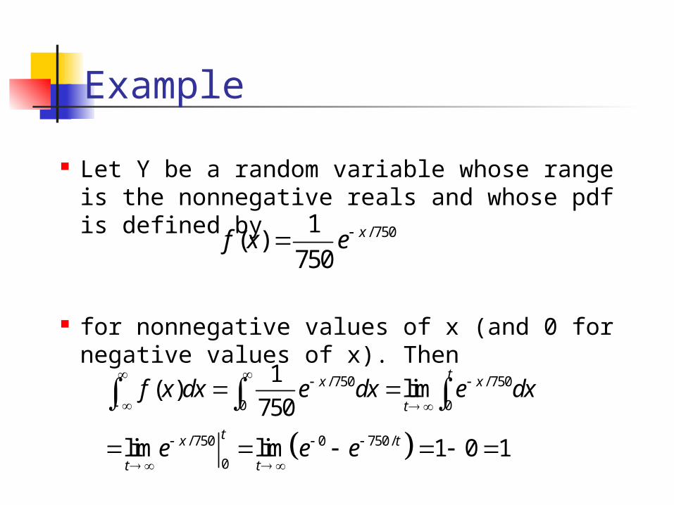
Let Y be a random variable whose range is the nonnegative reals and whose pdf is defined by

for nonnegative values of x (and 0 for negative values of x). Then

/ 7501( )

750xf x e

/ 750 / 750

0 0

/ 750 0 750/

0

1( ) lim

750

lim lim 1 0 1

tx x

t

tx t

t t

f x dx e dx e dx

e e e

Cumulative Distribution Functions

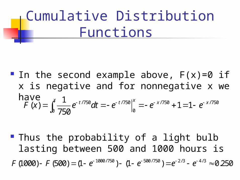
In the second example above, F(x)=0 if x is negative and for nonnegative x we have

Thus the probability of a light bulb lasting between 500 and 1000 hours is

/ 750 / 750 / 750 / 750

00

1( ) 1 1

750

x xt t x xF x e dt e e e

1000/ 750 500/ 750 2/3 4 /3(1000) (500) (1 ) (1 ) 0.250F F e e e e

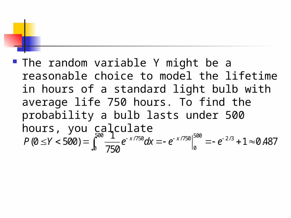
The random variable Y might be a reasonable choice to model the lifetime in hours of a standard light bulb with average life 750 hours. To find the probability a bulb lasts under 500 hours, you calculate

500 500/ 750 / 750 2/3

00

1(0 500) 1 0.487

750x xP Y e dx e e

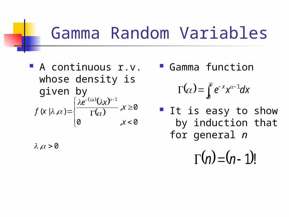
Gamma Random Variables

A continuous r.v. whose density is given by

Gamma function

It is easy to show by induction that for general n

0,

0,0

0,),|(

1

x

xxe

xf

x

0

1dxxe x

!1 nn

And And

0

110

1

0

1

0

1

1 dtetket

det

dtet)k(

tktk

tk

tk )( 2

1

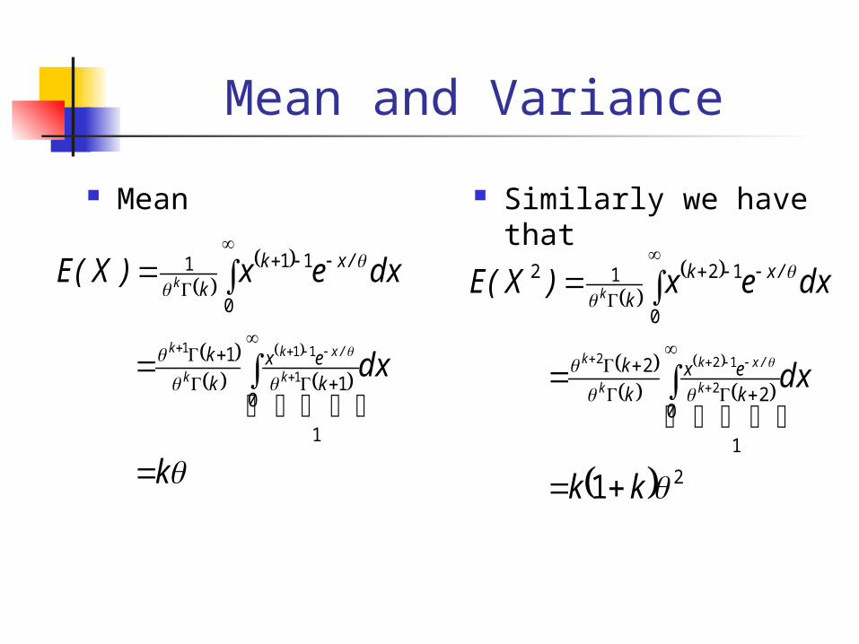
Mean and Variance

Mean Similarly we have that

k

dx

dxex)X(E

kex

k

k

/xk

k

k

/xk

k

k

k

1

01

1

0

111

1

111

2

1

02

2

0

1212

1

2

122

kk

dx

dxex)X(E

kex

k

k

/xk

k

k

/xk

k

k

k

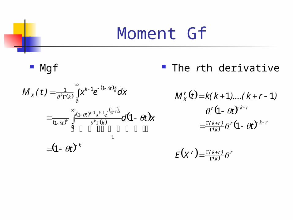
Moment Gf

Mgf The rth derivative

k

k

ext

t

tk

kX

t

xtd

dxex)t(M

k

xtkk

k

x

k

1

1

1

0

1

1

0

111

111

r

k)rk(r

rkrk

)rk(

rkr

rX

XE

t

t

)rk)....(k(ktM

1

1

11

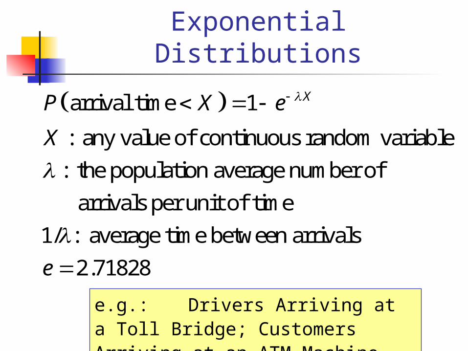
Exponential Distributions

arrival time 1

: any value of continuous random variable

: the population average number of

arrivals per unit of time

1/ : average time between arrivals

2.71828

XP X e

X

e

e.g.: Drivers Arriving at a Toll Bridge; Customers Arriving at an ATM Machine

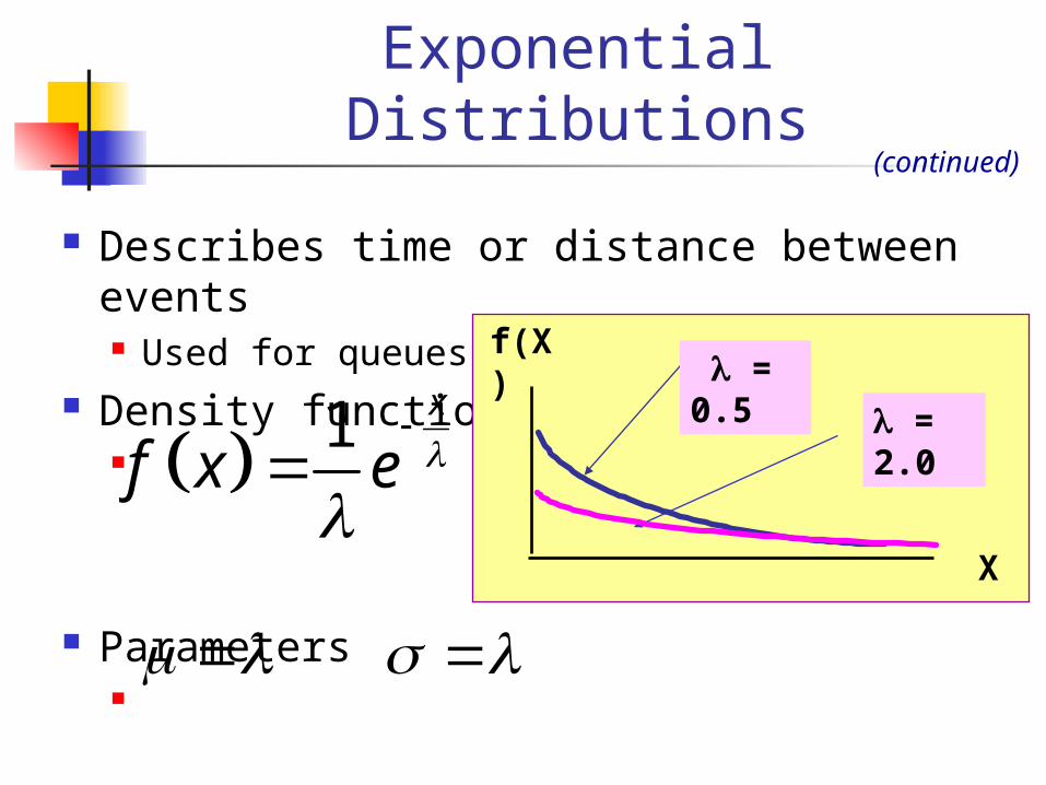
Exponential Distributions

Describes time or distance between events Used for queues

Density function

Parameters

(continued)

f(X)

X

= 0.5

= 2.0

1 x

f x e

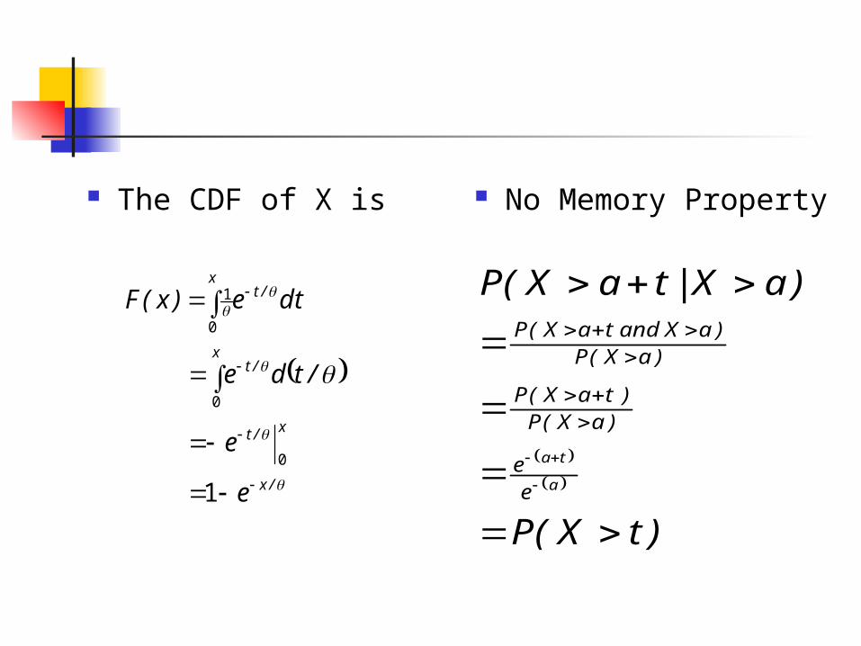
The CDF of X is No Memory Property

/x

x/t

x/t

/tx

e

e

/tde

dte)x(F

1

0

0

0

1

)tX(P

)aX|taX(P

a

ta

ee

)aX(P)taX(P

)aX(P)aXandtaX(P

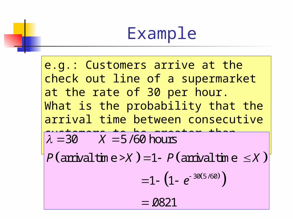
Example

e.g.: Customers arrive at the check out line of a supermarket at the rate of 30 per hour. What is the probability that the arrival time between consecutive customers to be greater than five minutes?

30 5/ 60

30 5 / 60 hours

arrival time > 1 arrival time

1 1

.0821

X

P X P X

e

Exponential Distribution in PHStat

PHStat | probability & prob. Distributions | exponential

Example in excel spreadsheet

Microsoft Excel Worksheet

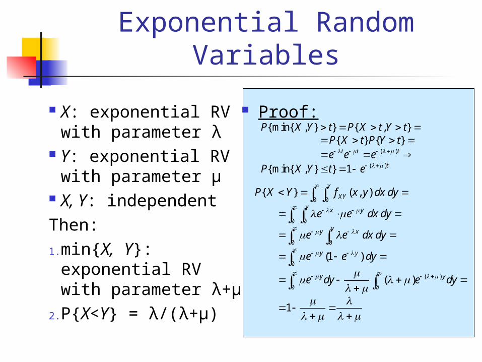
Exponential Random Variables

X: exponential RV with parameter λ

Y: exponential RV with parameter μ

X, Y: independentThen:1. min{X, Y}: exponential

RV with parameter λ+μ

2. P{X<Y} = λ/(λ+μ)

Proof:

0 0

0 0

0 0

0

( )

0 0

{ } ( , )

(1 )

( )

1

y

XY

yx y

yy x

y y

y y

P X Y f x y dx dy

e e dx dy

e e dx dy

e e dy

e dy e dy

( )

( )

{min{ , } } { , }{ } { }

{min{ , } } 1

t t t

t

P X Y t P X t Y tP X t P Y te e e

P X Y t e

Weibull Distribution

A continuous r.v. X is said to have the Weibull distribution with parameters ß,Ø>0 if it has a pdf of the form

It follows that the 100 x pth percentile has the form

01,,

0,,

/

/1

xexF

xexxf

x

x

.1ln /1 px

pxF

p

p

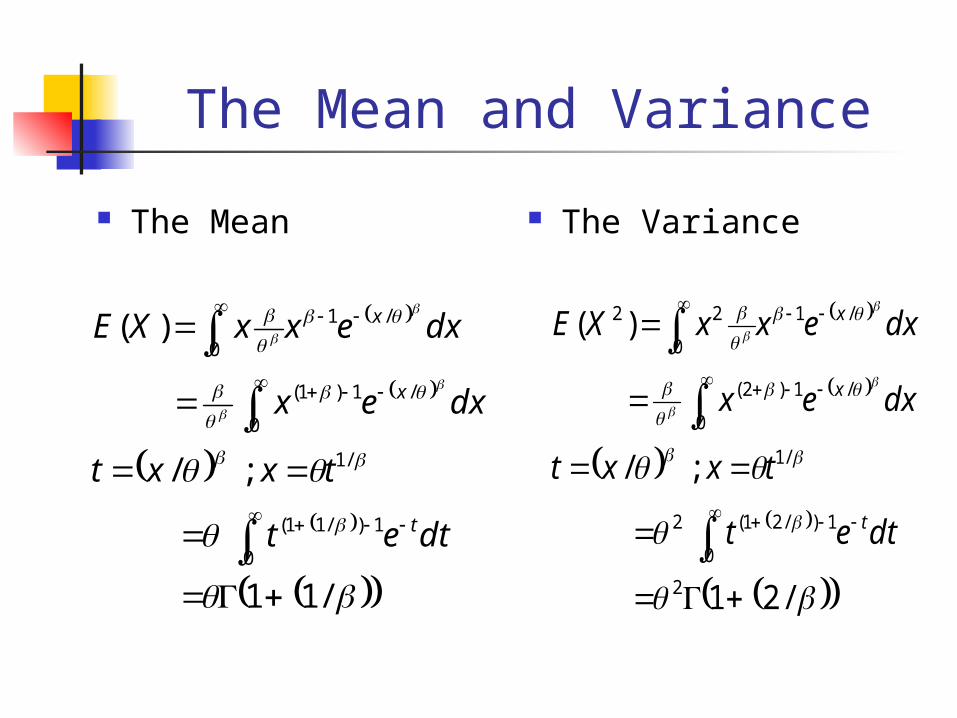
The Mean and Variance

The Mean The Variance

/11

;/

)(

0

1)/11(

/1

0

/1)1(

/1

0

dtet

txxt

dxex

dxexxXE

t

x

x

/21

;/

)(

2

0

1)/21(2

/1

0

/1)2(

/1

0

22

dtet

txxt

dxex

dxexxXE

t

x

x

The Normal Distribution

“Bell shaped” Symmetrical Mean, median and

mode are equal Interquartile range

equals 1.33 Random variable

has infinite range

Mean Median Mode

X

f(X)

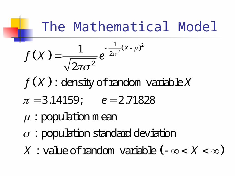
The Mathematical Model

21

2

2

1

2

: density of random variable

3.14159; 2.71828

: population mean

: population standard deviation

: value of random variable

X

f X e

f X X

e

X X

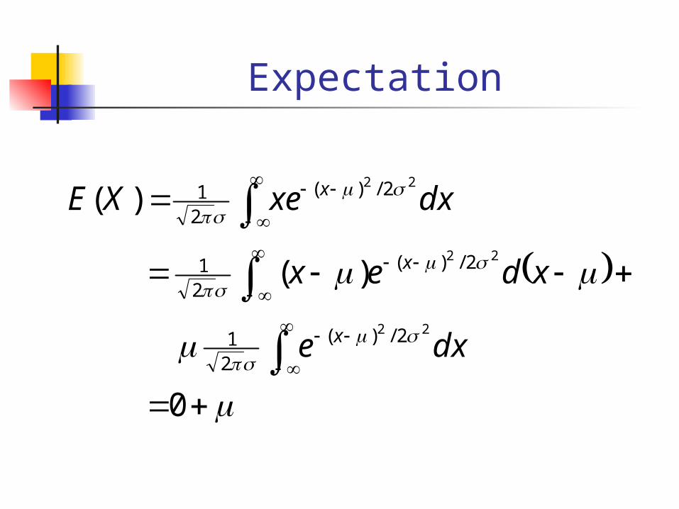
Expectation

0

)(

)(

22

22

22

2/)(

21

2/)(

21

2/)(

21

dxe

xdex

dxxeXE

x

x

x

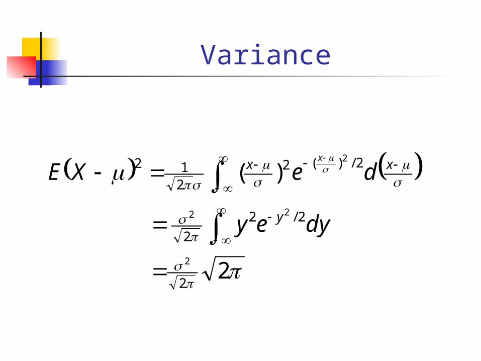
Variance

2

)(

2

2/2

2

2/)(2

212

2

22

2

dyey

deXE

y

xxx

Many Normal Distributions

By varying the parameters and , we obtain different normal distributions

There are an infinite number of normal distributions

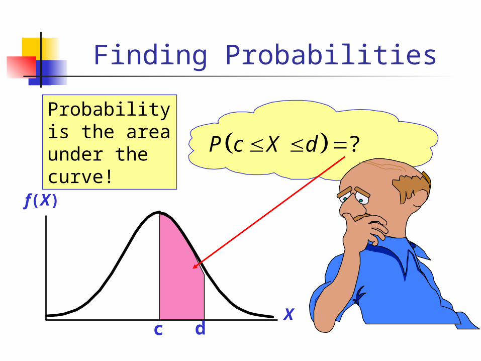
Finding Probabilities

Probability is the area under the curve!

c dX

f(X)

?P c X d

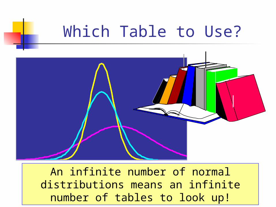
Which Table to Use?

An infinite number of normal distributions means an infinite number of tables to look

up!

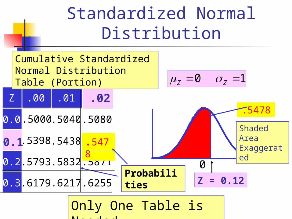
Solution: The Cumulative Standardized Normal

Distribution

Z .00 .01

0.0 .5000 .5040 .5080

.5398 .5438

0.2 .5793 .5832 .5871

0.3 .6179 .6217 .6255

.5478.02

0.1 .5478

Cumulative Standardized Normal Distribution Table (Portion)

Probabilities

Shaded Area Exaggerated

Only One Table is Needed

0 1Z Z

Z = 0.12

0

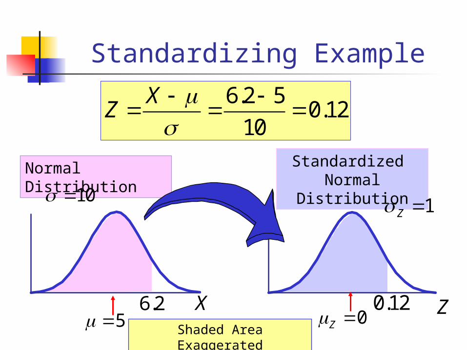
Standardizing Example

6.2 50.12

10

XZ

Normal Distribution

Standardized Normal

Distribution


10 1Z

5 6.2 X Z0Z

0.12

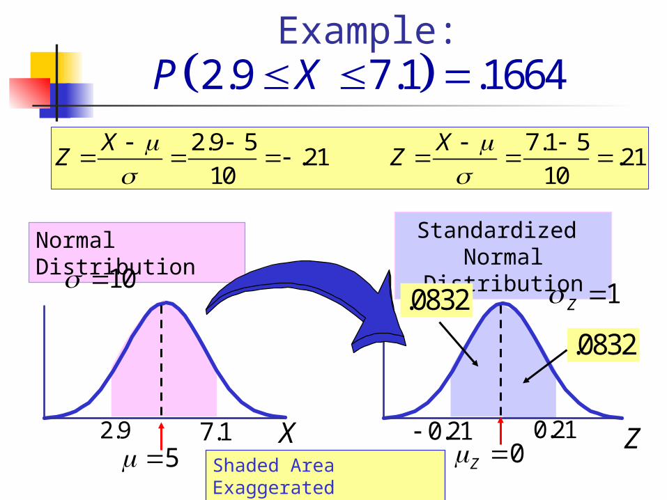
Example:

Normal Distribution

Standardized Normal

Distribution


10 1Z

5 7.1 X Z0Z

0.21

2.9 5 7.1 5.21 .21

10 10

X XZ Z

2.9 0.21

.0832

2.9 7.1 .1664P X

.0832

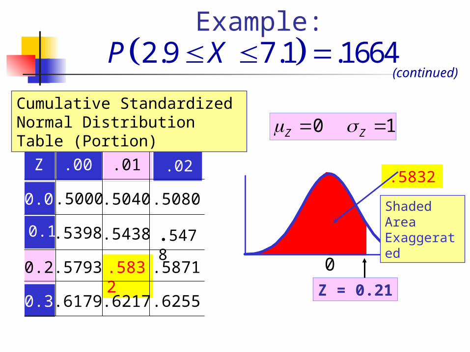
Z .00 .01

0.0 .5000 .5040 .5080

.5398 .5438

0.2 .5793 .5832 .5871

0.3 .6179 .6217 .6255

.5832.02

0.1 .5478



0 1Z Z

Z = 0.21

Example: 2.9 7.1 .1664P X

(continued)

0

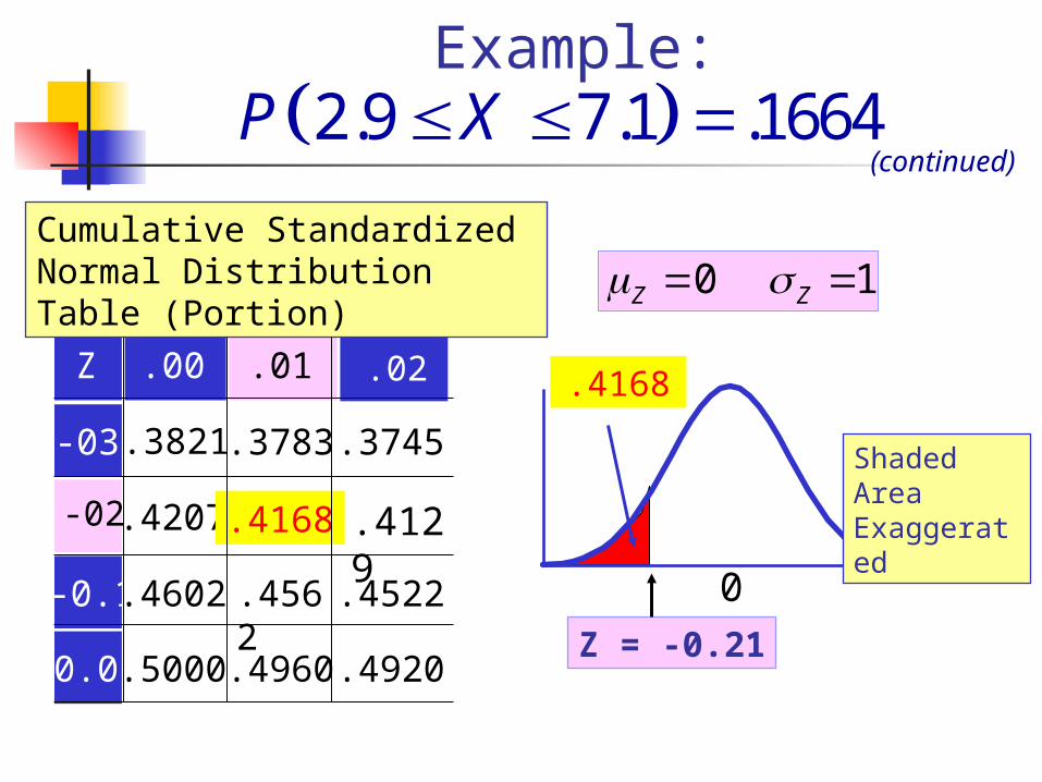
Z .00 .01

-03 .3821 .3783 .3745

.4207 .4168

-0.1.4602 .4562 .4522

0.0 .5000 .4960 .4920

.4168.02

-02 .4129



0 1Z Z

Z = -0.21

Example: 2.9 7.1 .1664P X

(continued)

0

Normal Distribution in PHStat

PHStat | probability & prob. Distributions | normal …

Example in excel spreadsheet

Microsoft Excel Worksheet

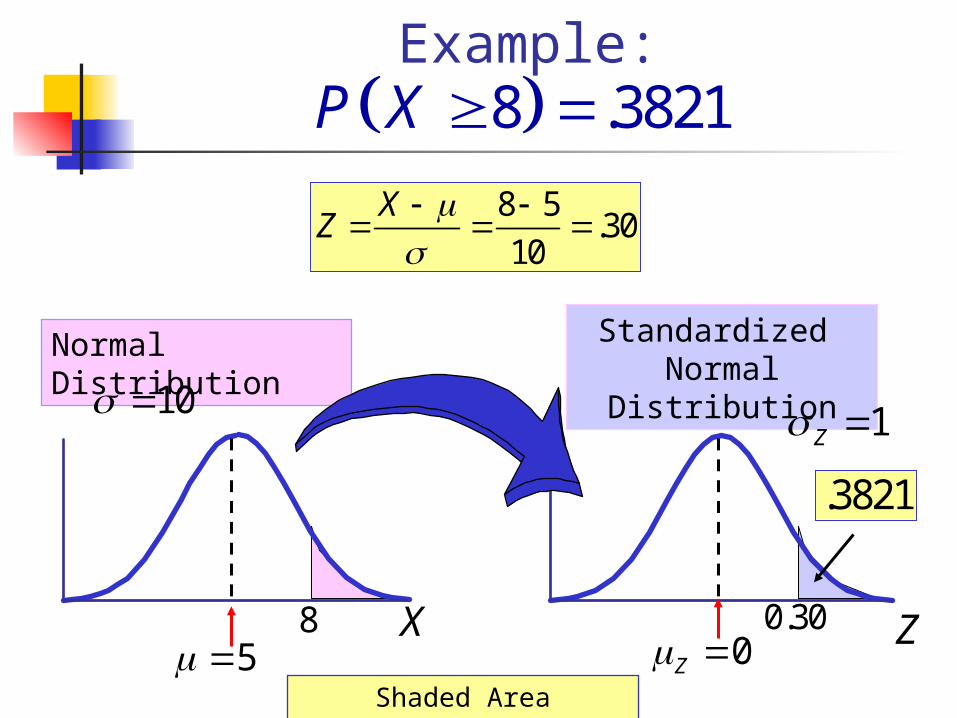
Example: 8 .3821P X

Normal Distribution

Standardized Normal

Distribution


10 1Z

5 8 X Z0Z

0.30

8 5.30

10

XZ

.3821

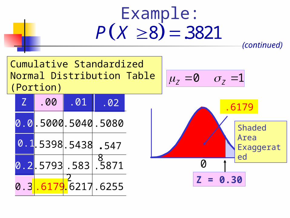
Example: 8 .3821P X

(continued)

Z .00 .01

0.0 .5000 .5040 .5080

.5398 .5438

0.2 .5793 .5832 .5871

0.3 .6179 .6217 .6255

.6179.02

0.1 .5478



0 1Z Z

Z = 0.30

0

.6217

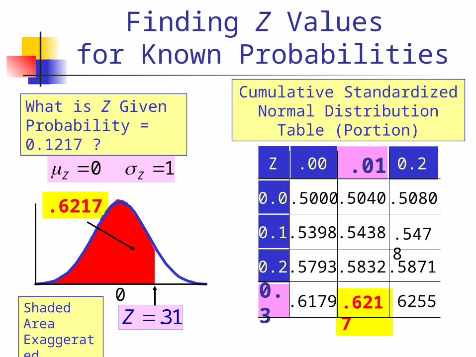
Finding Z Values for Known Probabilities

Z .00 0.2

0.0 .5000 .5040 .5080

0.1 .5398 .5438 .5478

0.2 .5793 .5832 .5871

.6179 .6255

.01

0.3

Cumulative Standardized Normal Distribution Table

(Portion)

What is Z Given Probability = 0.1217 ?


.6217

0 1Z Z

.31Z 0

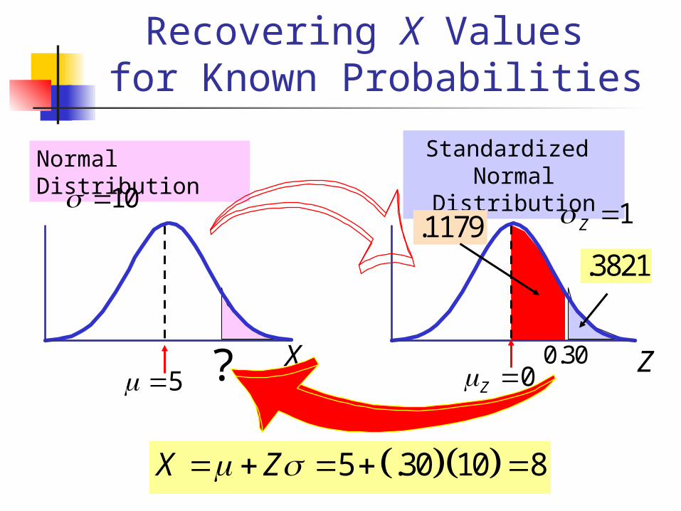
Recovering X Values for Known Probabilities

5 .30 10 8X Z

Normal Distribution

Standardized Normal

Distribution10 1Z

5 ? X Z0Z 0.30

.3821.1179

Assessing Normality

Not all continuous random variables are normally distributed

It is important to evaluate how well the data set seems to be adequately approximated by a normal distribution

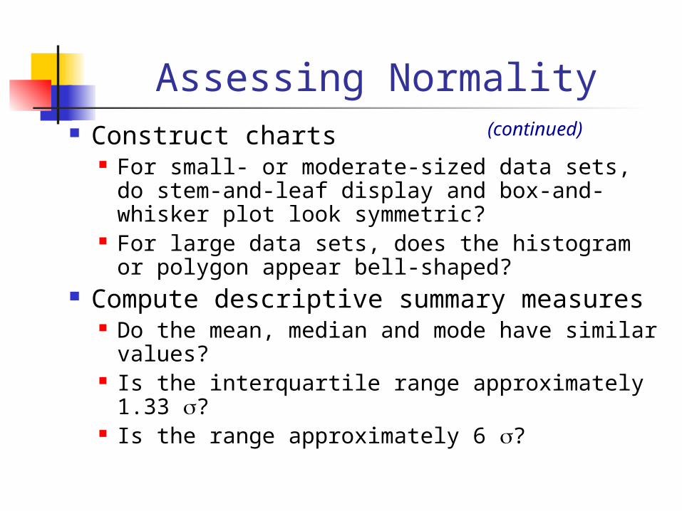
Assessing Normality Construct charts

For small- or moderate-sized data sets, do stem-and-leaf display and box-and-whisker plot look symmetric?

For large data sets, does the histogram or polygon appear bell-shaped?

Compute descriptive summary measures Do the mean, median and mode have similar

values? Is the interquartile range approximately 1.33 ?

Is the range approximately 6 ?

(continued)

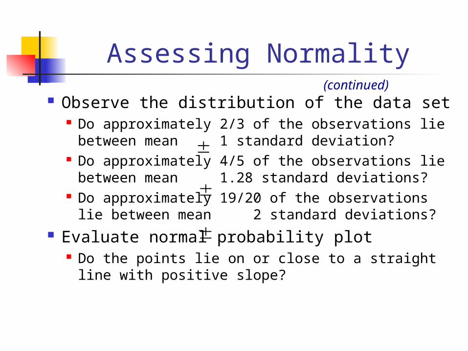
Assessing Normality

Observe the distribution of the data set Do approximately 2/3 of the observations lie

between mean 1 standard deviation? Do approximately 4/5 of the observations lie

between mean 1.28 standard deviations? Do approximately 19/20 of the observations

lie between mean 2 standard deviations? Evaluate normal probability plot

Do the points lie on or close to a straight line with positive slope?

(continued)

Assessing Normality

Normal probability plot Arrange data into ordered array Find corresponding standardized normal

quantile values Plot the pairs of points with observed data

values on the vertical axis and the standardized normal quantile values on the horizontal axis

Evaluate the plot for evidence of linearity

(continued)

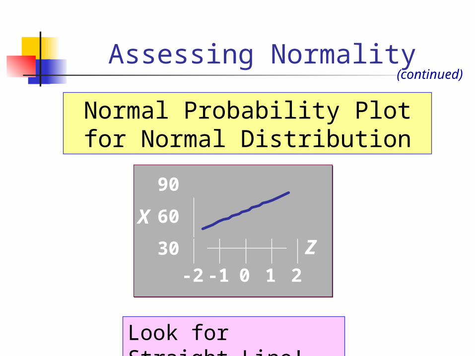
Assessing Normality

Normal Probability Plot for Normal Distribution

Look for Straight Line!

30

60

90

-2 -1 0 1 2

Z

X

(continued)

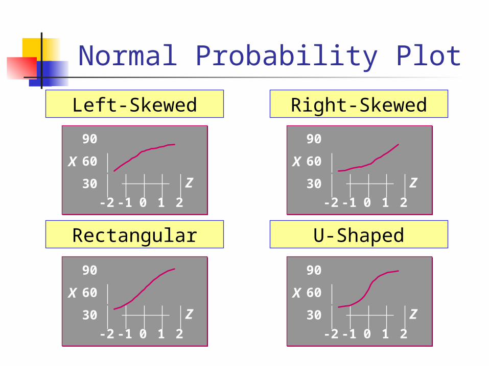
Normal Probability Plot

Left-Skewed Right-Skewed

Rectangular U-Shaped

30

60

90

-2 -1 0 1 2

Z

X

30

60

90

-2 -1 0 1 2

Z

X

30

60

90

-2 -1 0 1 2

Z

X

30

60

90

-2 -1 0 1 2

Z

X

Documents

Chap3b.continuous Distrib