Scattering Theory

P. Thangadurai

Scattering and Cross Section

Importance of ScatteringMuch of our understanding about the structure of matter is extracted from the scattering of particles. Without scattering, the structure of the microphysical world would haveremained inaccessible to humans. It is through scattering experiments that important building blocks of matter, such as the atomic nucleus, the nucleons, and the various quarks, have been discovered.

Importance of Scattering

• In a scattering experiment, one observes the collisions between a beam of incident particles and a target material.

• The total number of collisions over the duration of the experiment is proportional to the total number of incident particles and to the number of target particles per unit area in the path of the beam.

•In these experiments, one counts the collision products that come out of the target.After scattering, some will go undisturbed those particles that do not interact with the target continuetheir motion (undisturbed) in the forward direction, but those that interact with the target get scattered (deflected) at some angle as depicted in Figure 11.1.

The number of particles coming out varies from one direction to the other.

The number of particles scattered into an element of solid angle d (d =dq sinqdj) is proportional to a quantity that plays a central role in the physics of scattering: the differential cross section.

Differential cross section.

The differential cross section, which is denoted by d(q , j )/d , is defined as the number of particles scattered into an element of solid angle d in the direction (q , j )per unit time and incident flux:

( , ) 1 ( , )

inc

d dN

d J d

q j q j

where Jinc is the incident flux (or incident current density); it is equal to the number of incident particles per area per unit time.

We can verify that d/d has the dimensions of an area; hence it is appropriate to call it a differential cross section.

--------(A)

The relationship between d/d and the total cross section is obvious:

--------(B)

The scattering amplitude f (q , j ) plays a central role in the theory of scattering, since it determines the differential cross section.To see this, let us first introduce the incident and scattered flux densities:

Scattering Amplitude and Differential Cross Section

In this case behaves as a free particle before collision and hence can be described by a plane wave (k0 and k are the wave vectors of incident and scattered waves respectively)

--------(1)

--------(2)

--------(3)

--------(4)

Inserting (3) into (1), 0

0

0

0

.

.*

.

.*

( )( )( ) ( )( ) ( )

ik rinc

ik rinc

ik rinc

ik rinc

r Aer Aer ik Aer ik Ae

* *

2inc inc inc inc inc

iJ

* *

2sc sc sc sc sc

iJ

0 .( ) ik rinc r Ae

.

( ) ( , )ik r

sc

er Af

r q j

After the scattering has taken place, the total wave consists of a superposition of the incident plane wave (3) and the scattered wave (4):

0

..( ) ( ) ( ) ( , )

ik rik r

inc sc

er r r A e f

r q j

--------(4a)

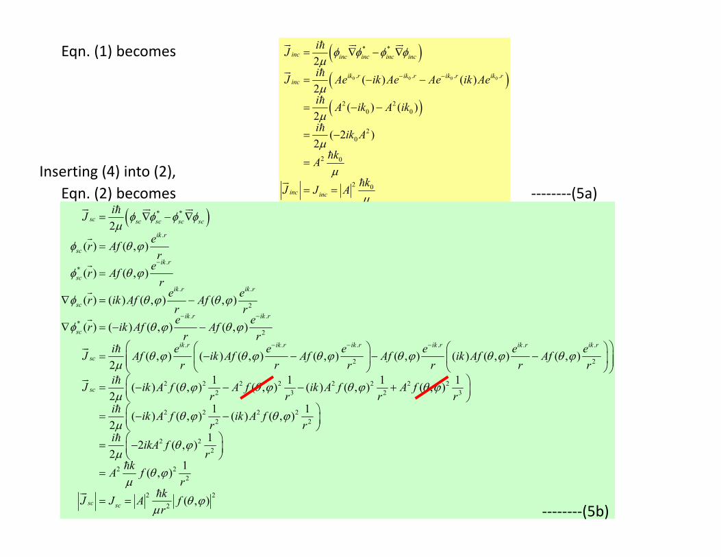
Eqn. (1) becomes

0 0 0 0

* *

. . . .

2 20 0

20

2 0

2 0

2

( ) ( )2

( ) ( )2

( 2 )2

inc inc inc inc inc

ik r ik r ik r ik rinc

inc inc

iJ

iJ Ae ik Ae Ae ik Ae

iA ik A ik

iik A

kA

kJ J A

* *

.

.*

. .

2

. .*

2

.

2

( ) ( , )

( ) ( , )

( ) ( ) ( , ) ( , )

( ) ( ) ( , ) ( , )

( , ) ( ) ( , )2

sc sc sc sc sc

ik r

sc

ik r

sc

ik r ik r

sc

ik r ik r

sc

ik r ik

sc

iJ

er Af

re

r Afre e

r ik Af Afr re e

r ik Af Afr r

i e eJ Af ik Af

r

q j

q j

q j q j

q j q j

q j q j

. . . . .

2 2

2 2 2 2 2 2 2 2

2 3 2 3

2 2 2 2

2

( , ) ( , ) ( ) ( , ) ( , )

1 1 1 1( ) ( , ) ( , ) ( ) ( , ) ( , )

21 1

( ) ( , ) ( ) ( , )2

r ik r ik r ik r ik r

sc

e e e eAf Af ik Af Af

r r r r r

iJ ik A f A f ik A f A f

r r r ri

ik A f ik A fr r

q j q j q j q j

q j q j q j q j

q j q j

2

2 2

2

2 2

2

2 2

2

12 ( , )

21

( , )

( , )sc sc

iikA f

rk

A fr

kJ J A f

r

q j

q j

q j

Eqn. (2) becomes

Inserting (4) into (2),

--------(5a)

--------(5b)

Now, we may recall that the number dN (q , j) of particles scattered into an element of solid angle d in the direction (q , j )and passing through a surface element dA = r2d per unit time is given as follows (see Eqn.1):

where Jsc is the scattered flux (or incident current density); it is equal to the number of incident particles per area per unit time.

2( , ) scdN J r dq j --------(6)

Using equantion (5b) in (6), we get

2

2 2 2

2

2 2

( , )

( , )

( , )( , )

sc

dNJ r

dk

A f rr

dN kA f

d

q j

q j

q jq j

--------(7)

Substitute Eq. (7) and Jinc from fromEq.(5a) in (1)

2 2

2 0

2

0

( , ) 1 ( , )

1( , )

( , )( , )

inc

d dN

d J dk

A fk

A

d kf

d k

q j q j

q j

q jq j

--------(8)

Since the normalization factor A does not contribute to the differential cross section, we will be taking it equal to one.

For elastic scattering k0 is equal to k; hence (8) reduces to

2( , )( , )

df

d

q jq j

The problem of determining the differential cross section d/d therefore reduces to that of obtaining the scattering amplitude f (q , j )

--------(9)

Scattering Amplitude, f(q,j)Consider elastic scattering of two particles of mass m1 and m2 (spinless, non-relativistic). We are going to show here that we can obtain the differential cross section for this case in the CM frame from an asymptotic form of the solution of the Schrödinger equation (Eq. 10).

Let us first focus on the determination of f(q,j); it can be obtained from the solutions of Schrodinger Eqn.

22 ( ) ( ) ( ) ( )

2r V r r E r

m

--------(10)

This eqn is a reduced form of eqn explaining the elastic scattering of two particles of mass m1 and m2 (spinless, non-relativistic). Scattering between two particles is thus reduced to solving this equation (See page 622 of Zettili Book).

Eq (10) can be rewritten as

2 2 2

2 2

2 2( ) ( ) ( ) ( ), where k r V r r k E

--------(11)

The general solution to this equation consists of a sum of two components: a general solution to the homogeneous equation:

2 2homo( ) ( ) 0k r --------(12)

and a particular solution to Eqn. (11). Note that homo(r) is nothing but the incident plane as given in Eq. (4)

As for the particular solution to Eq.(11), we can express it in terms of Green’s function. Thus, the general solution of Eq. (11) is given by

3

2

2( ) ( ) ( ') ( ') ( ') 'incr r G r r V r r d r

--------(13)

is Green’s function corresponding to the operator on the left-hand side of (12).

0 .( ) ik rinc r Ae

where and ( ')G r r

Green’s function is obtained by solving the point source equation and the Green’s function for the scattered wave (outgoing wave) is given as

'1

( ')4 '

ik r re

G r rr r

--------(14)

Inserting this in eqn (13) we get, '

3

2( ) ( ) ( ') ( ') '

2 '

ik r r

inc

er r V r r d r

r r

--------(15)

0

.. ( , ) as r

ik rik r ee f

r q j

--------(16)

. ' 3

2, ( ') ( ') '

2ik rf e V r r d r

q j

Where, --------(17)

The differential cross section is then given by

2 22 . ' 3

2 4, ( ') ( ') '

4ik rd

f e V r r d rd

q j

-----(18)

The First Born Approximation

If the potential V(r) is weak enough, it will distort only slightly the incident plane wave. The first Born approximation consists then of approximating the scattered wave function (r)by a plane wave.

This approximation corresponds to the first iteration of (15); that is, (r) is given by:'

3

2( ) ( ) ( ') ( ') '

2 '

ik r r

inc inc

er r V r r d r

r r

--------(19)

Thus, using (17) and (18), we can write the scattering amplitude and the differential cross section in the first Born approximation as follows:

. ' 3

2

. ' 3

2

, ( ') ( ') '2

, ( ') '2

ik rinc

iq r

f e V r r d r

f e V r d r

q j

q j

0

0 0

0

. '

0

. ' . ' . ' . '

( - ). ' . '

( ')Here -

Therefore, ( ') ( ')( ') ( ')

ik rinc

ik r ik r ik r ik r

i k k r iq r

r eq k k

e V r e e V r ee V r e V r

------(20)

2 22 . ' 3

2 4, ( ') '

4iq rd

f e V r d rd

q j

The differential cross section

------(21)

where q = k0 k and ħq is the momentum transfer; ħk0 and ħk are the linear momenta of the incident and scattered particles, respectively.

In elastic scattering, the magnitudes of k0 = k (Figure 11.6); hence

0

2 20 0

2 2 2

2

2 2

-

2 cos

2 cos

2 (1 cos )

2 2sin ( cos 2 1 2sin )2

2 sin2

q q k k

k k kk

k k k

k

k

q k

q

q

q

qq q

q

Modulus of q ------(22)

------(23)

If the potential is spherically symmetric, and choosing the z-axis along q (Figure 11.6), then

( ')V r

( ') ( )V r V r

and therefore the integral part of Eq. (21) becomes

. ' 'cos 'q r qr q

. ' 3 'cos ' 2

22 'cos '

0 0 0

( ') ' ( ') ' 'sin ' ' '

' ( ') ' sin ' ' '

iq r iqr

iqr

e V r d r e V r r dr d d

r V r dr e d d

q

q

q q j

q q j

2

0

' 2d

j

'cos '

0

11 ''cos ' '

0 1 1

' '

'

Take cos ' sin ' '

sin ' 'when =0, x = 1 and = , x = -1

''

1

'1

2 sin( ')'

12sin( ')

'

iqr

iqr xiqr iqr x

iqr iqr

e d

xdx ddx d

ee d e dx

iqr

e eiqr

i qriqr

qrqr

q

q

q

qq q

q qq q

q

2

0 0

1 2' ( ') 2sin( ') ' ' ( ') sin( ') '

'r V r qr dr r V r qr dr

qr q

= 2 1

2sin( ')'

qrqr

. ' 3

0

4( ') ' ' ( ') sin( ') 'iq re V r d r r V r qr dr

q

Therefore

------(24)

3 2Volume element in 3-D spherical coordinates

sind r r drd dq q

Inserting (24) into (20) we obtain

2

0

4' ( ') sin( ') '

2f r V r qr dr

q

q

------(25)

Inserting (25) into (21) we obtain

2

22

2 4

0

4' ( ') sin( ') '

df r V r qr dr

d q

q

In summary, • The Schrödinger equation (11.30) is solved with first-order Born approximation (where the

potential V(r’) is weak enough that the scattered wave function is only slightly different from the incident plane wave)

• The scattering amplitude (Eqn.25)and the differential cross section (Eqn.25) were obtained for for a spherically symmetric potential.

2

0

2' ( ') sin( ') 'f r V r qr dr

q

q

------(26)

The first Born approximation is valid whenever the wave function (r) is only slightly differentfrom the incident plane wave

That is, whenever the second term in Eq. (19) is very small compared to the first:

'

3

2( ) ( ) ( ') ( ') '

2 '

ik r r

inc inc

er r V r r d r

r r

--------(19)

'2

3

2( ') ( ') ' ( )

2 '

ik r r

inc inc

eV r r d r r

r r

0

0 0

.

2. .

Since ( )

( ) 1

ik rinc

ik r ik rinc

r e

r e e

'

3

2( ') ( ') ' 1

2 '

ik r r

inc

eV r r d r

r r

In elastic scattering k0 = k and assuming that the scattering potential is largest near r = 0, we have (following the same integration procedure followed for Eqn. (24) and putting r = 0),

--------(20)

--------(21)

' 'cos '

2

0 0

' ( ') ' sin ' ' 1ikr ikrr e V r dr e d

qq q

'cos '

0

11 ''cos ' '

0 1 1

' '

'

Take cos ' sin ' '

sin ' 'when =0, x = 1 and = , x = -1

''

1

'

ikr

ikr xikr ikr x

ikr ikr

e d

xdx ddx d

ee d e dx

ikr

e eikr

q

q

q

qq q

q qq q

q

--------(22)

Since the energy of the incident particle is proportional to k (it is purely kinetic, )we infer from (22) thatthe Born approximation is valid for large incident energies and weak scattering potentials.

That is, when the average interaction energy between the incident particle and the scattering potential is much smaller than the particle’s incident kinetic energy, the scattered wave can be considered to be a plane wave.

2 2E k

• So far we have considered only an approximate calculation of the differential cross section where the interaction between the projectile particle and the scattering potential V(r) is considered small compared with the energy of the incident particle.

• In this section we are going to calculate the cross section without placing any limitation on the strength of V(r)

Partial Wave Analysis for Elastic Scattering

• We assume here the potential to be spherically symmetric. • (In the special case of a central potential V(r), the orbital angular momentum L of the

particles is a constant of motion. Therefore, there exist stationary states with well defined angular momentum: that is, eigen states commone to H, L2, Lz. We shall call the wave functions associated with these states PARTIAL WAVES. )

• The angular momentum of the incident particle will therefore be conserved; a particle scattering from a central potential willhave the same angular momentum before and after collision.

• Assuming that the incident plane wave is in the z-direction and hence

cos( ) ikrinc r e q

--------(22)

we may express it in terms of a superposition of angular momentum eigenstates, each with a definite angular momentum number l

. cos

0

(2 1) ( ) (cos )ik r ikr ll l

l

e e i l j kr Pq q

--------(23)

We can then examine how each of the partial waves is distorted by V(r) after the particle scatters from the potential. [jl(kr) is the Bessel Function]

The most general solution of the Schrödinger equation (10) is

Consider the Schrödinger equation in CM frame: (Eq. 10)2

2 ( ) ( ) ( ) ( )2

r V r r E rm

--------(10)

( ) ( ) ( , )lm kl lmlm

r C R r Y q j

--------(24)

Since V(r ) is central, the system is symmetrical (rotationally invariant) about the z-axis. The scattered wave function must not then depend on the azimuthal

angle j; m =0. Thus, as Yl0q,j~Pl (cosq), the scattered wave function Eq.(24) becomes

0

( , ) ( ) (cos )l kl ll

r a R r P q q

--------(25)

Each term in (25), which is known as a partial wave, is a joint eigenfunction of L2 and LZ .

where Rkl (r ) obeys the following radial equation

2 2

2 2 2 2

( 1) 2 2( ( )) ( )( ( )) , where

d l l m Ek rRkl r V r rRkl r k

dr r

--------(26)

0

..( ) ( ) ( ) ( , )

ik rik r

inc sc

er r r A e f

r q j

A substitution of (23) [for into

--------(4a)

with j=0 (and k=k0 for elastic scattering) gives

( )inc r

.

0

( , ) ( ) ( ) (2 1) ( ) (cos ) ( )ik r

linc sc l l

l

er r r i l j kr P f

r q q q

--------(27)

The scattered wave function is given, on the one hand, by (25) and, on the other hand, by (27).

Consider the limit r

1) Since in almost all scattering experiments detectors are located at distances from thetarget that are much larger than the size of the target itself.

The limit of the Bessel function jl(kr) for large values of r is given by

sin( / 2)( ) ( )l

kr lj kr r

kr

--------(28)

the asymptotic form of (27) is given by

.

0

sin( / 2)( , ) ( ) ( ) (2 1) (cos ) ( )

ik rl

inc sc ll

kr l er r r i l P f

kr r

q q q

--------(29)

one can write (29) as

/2 /2since, sin( / 2) [( 1) ] / 2because, ( ) ( )

l ikr l ikr

il i l lkr l e i e ie e i

0

2

0 0

[( 1) ] / 2( , ) (2 1) (cos ) ( )

1( , ) (2 1) (cos ) ( ) ( )(2 1) (cos )

2 2

l ikr l ikr ikrl

ll

ikr ikrl l l

l ll l

e i e i er i l P f

kr re e

r i l P f i i l Pikr r ik

q q q

q q q q

------(30)

2) To find the asymptotic form of (25), we need first to determine the asymptotic form of the radial function Rkl (r ). At large values of r, the scattering potential is effectively zero radial equation (26) becomes

2

2( ( )) 0

dk rRkl r

dr

------(31)

The general solution of this equation is given by a linear combination of the sphericalBessel and Neumann functions

--------(29a)

we can write the asymptotic limit of the scattered wave function (25) as

0

sin( / 2 )( , ) (cos ) ( )l

l ll

kr lr a P r

kr

d q q

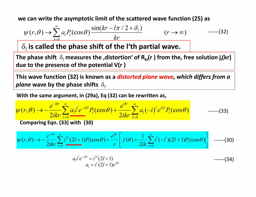
------(32)

dl is called the phase shift of the l‘th partial wave.

The phase shift dl measures the ‚distortion‘ of Rkl(r ) from the‚ free solution jl(kr) due to the presence of the potential V(r )

This wave function (32) is known as a distorted plane wave, which differs from a plane wave by the phase shifts dl

With the same argument, in (29a), Eq (32) can be rewritten as,

0 0

( , ) (cos ) ( ) (cos )2 2

ikr ikrl i l l i l

l l l ll l

e er a i e P a i e P

ikr ikrd d q q q

------(33)

Comparing Eqn. (33) with (30)

2

0 0

1( , ) (2 1) (cos ) ( ) ( )(2 1) (cos )

2 2

ikr ikrl l l

l ll l

e er i l P f i i l P

ikr r ik q q q q

------(30)

2 (2 1)(2 1)

l i l ll

l i ll

a i e i la i l e

d

d

------(34)

Substituting al in (33)

2

0 0

( , ) (2 1) (cos ) (2 1) ( ) (cos )2 2

ikr ikrl i l l i l l i l l

l ll l

e er i l e i e P i l e i P

ikr ikrd d d q q q

------(35)

Equating the coefficient of in (30) with (35), we haveikre

r

2

0 0

1 1( ) ( )(2 1) (cos ) (2 1) ( ) (cos )

2 2l l l l i l

l ll l

f i i l P l i i e Pik ik

dq q q

------(36)

From (30) From (33)

2, ( 1) / 2 ( ) / 2(cos sin cos sin ) / 2(2 sin ) / 2sin

i l i l i l i l

i l

i l

i l

Since e i e e e ie l i l l i l ie i l ie l

d d d d

d

d

d

d d d dd

d

Rearranging (36)2 2

0 0 0

2

0

1 1( ) ( ) (2 1) ( ) (cos ) ( )(2 1) (cos ) [since ( ) ( ) 1]

2 21

( ) (2 1) (cos )( 1)2

l l i l l l l l ll l l

l l l

i ll

l

f f l i i e P i i l P i i iik ik

f l P eik

d

d

q q q q

q q

0

1( ) (2 1) sin (cos )i l

ll

f l e lPk

dq d q

------(37)

where fl(q) is denoted as the partial wave amplitude.

From (37) we obtain the differential cross sections

'2 ( )

' '20 ' 0

1(2 1)(2 ' 1) sin sin (cos ) (cos )l li

l l l ll l

df l l e P P

d kd d

q d d q q

• The differential cross section (38) consists of a superposition of terms with different angular momenta; this gives rise to interference patterns between different partial waves corresponding to different values of l.

• The interference terms go away in the total cross section when the integral

over qis carried out.

• Note that when V=0 everywhere, all the phase shifts ddl vanish, and hence the partial (38) is zero.

------(38)

**********