Embed Size (px)
Citation preview

Chap 3 - Digital Voltmeter

2
EIM Chap 3 – Digital Voltmeter
Digital voltmeter parameters
range
resolution
accuracy
input impedance
Digital voltmeter types
CC – continuous current
AC – alternative current
vector type
3
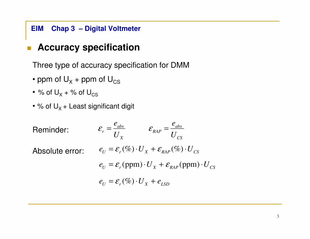
Three type of accuracy specification for DMM
• ppm of UX + ppm of UCS
• % of UX + % of UCS
• % of UX + Least significant digit
Reminder:
Absolute error:
EIM Chap 3 – Digital Voltmeter
Accuracy specification
abs absr RAP
X CS
e e
U Uε ε= =
(%) (%)U r X RAP CS
e U Uε ε= ⋅ + ⋅
(ppm) (ppm)U r X RAP CS
e U Uε ε= ⋅ + ⋅
(%)U r X LSD
e U eε= ⋅ +

4
EIM Chap 3 – Digital Voltmeter
Performances specification types
Keithley
GW-Instek

5
EIM Chap 3 – Digital Voltmeter
Relation between digits number (DMM) and bits number (DAC)
; ; cond:10 2
REF REFCS REF N n
U UU U V V V Vδ δ= ⇒ ∆ = = ∆ =
• ideal case
Exp:
• noisily case :
It uses
Exp:
DMM display N – digit number ΔV – display resolution
DAC n – bits number δV – conversion resol.
10 2log 4.92 5 ; log 16.33bitsCS CS
ech ech
U UN n
V Vδ
= = → = =
∆
1210 2
20V log 5.3 5 ; log 17.6bits ;
10μV
CS CS CSU U U
N nV V Vδ
= ⇒ = = → = =
∆ = ∆
_
_ _ , if unreliable12
noise MAX
RMS noise noise MAX
UU U V V= > ∆ → ∆
_ 12ech RMS noise
V U∆ = ⋅
_ ech70μV 70 12 μV=242.5μV=RMS noise ech
U V Vδ= → ∆ =

6
EIM Chap 3 – Digital Voltmeter
Digital voltmeter type

7
EIM Chap 3 – Digital Voltmeter
AO basic circuit (CIA remember)
Virtual Ground
0 ; ; 0f i
U IN i out
in i i
RV Va R R R
V R I= = − = = =
0 1 ; ; 0f
U IN out
in i
RVa R R
V R= = + → ∞ =
0 ; buffer functionin IN
V V R= → ∞ ⇒
Applications• Isolate one circuit from the loading effects of a following stage• Impedance converter - Data conversion System (ADC or DAC) where constant impedance or high impedance is required
Inverting amplifier
Non-inverting amplifier

8
EIM Chap 3 – Digital Voltmeter
AO basic circuit (CIA remember)
X LY X X X
L X L X
L X Y X
R RV V V V
R R R R
R R V V
= − =+ +
>> ⇒ ≈
Vx
Rx
Vy RLx
• open loop output: VX
• Voltage drop by load: VY
Ideal: RX low, RL very large
Differential amplifiers
( )
25 2
1 2
25 1 1 1 6 2 1
1
5 6 1 2
RV V
R RR
V V R I V V VR
V V I R
= +
= − ⇒ = −
= +

9
EIM Chap 3 – Digital Voltmeter
AO basic circuit (CIA remember)
• CMG = 0 ( V1=V2 V6=0V )
• DG = R2/R1
• CMRR = DG/CMG (large)
• not high input impedance ()
Instrumentation amplifier
• Two Noninvering Amp + One Differential Amp
• Differential Amp with High Input Impedance and
Low Output Impedance

10
EIM Chap 3 – Digital Voltmeter
Rectifiers
Precision half wave rectifier
Precision full wave rectifier
Limiters
2
10
, 0
, 0
i i
i i
Rv v
Rv
v v
− ≤
= >
2
10
, 0
0 , 0
i i
i
Rv v
Rv
v
− ≤
= >

11
EIM Chap 3 – Digital Voltmeter
D.C. digital voltmeter
Calibrated
dividerLPF
Dual Slope
ADCDisplay
UCS=200mV…2kV UCS=200mV
UX
Point position
UCS (dual slope ADC)=200mV

12
EIM Chap 3 – Digital Voltmeter
Calibrated voltmeter divider
10M - constantINR = Ω
200mV
H
200V
R390K
R19M
R49K
2V
Spre
V-metru
UCS=200mV
R2900K
L
20V
R51K
2000V
Selector scariBorne intrare
Ucs=200mV...
2000V
Input V-meterRange selector
mV-meter

13
Cal. divider electronic switch
Range: UCS = 200mV – 2V – 20V etc (range overlapping)
increasing: UIN = 0..200mV ⇒ UCS = 200mV
UIN = 200mV.. 2V ⇒ UCS = 2V
decreasing: UIN = 2V.. 180mV ⇒ UCS = 2V (decision hysteresis )
EIM Chap 3 – Digital Voltmeter
Auto-range digital d.c. voltmeter
Cal.
Div.
Overflow
det. logic
V-meter
UCS=200mV

14
EIM Chap 3 – Digital Voltmeter
Dual slope ADC
• Absolute values of R and C don’t affect operation
• Conversion time is given by:
• Digital output word gives average value of UX
during first integration phase
1 2 , ' n
CK x CKT T t N T= = ⋅
( )1 1
1
R
0
1 1d = d
+
∫ ∫XT T t
x
T
U t t V tRC RC
( )( )
11
' = = 2
2
−
=
⇒ = ⋅ = ⋅∑n
x ix
x R i RniR
U t t NU t V b V N
V T
( ) 12 ' 2 += + ≤n n
conv CK CKT N T T
• Example of schema for positive voltage

15
EIM Chap 3 – Digital Voltmeter
Dual slope ADC
1 2 , ' n
CK x CKT T t N T= = ⋅
( )1 1
1
1R
0
1 1+ d = - + d
2 2 2 2
XT T t
xR R R Rx x
T
tV V V V TU t t V t U
RC RC RC RC
+
− − ⇒ ⋅ = +
∫ ∫
1
1
1
1
0 for
= 0,5 for 02
0,5 for 2
x x
x
x R x R x
x R x
U t Tt T
U V U V t
U V t T
= =−
⇒ =− ⋅ = = ⋅ =
• Examples of scheme for bipolar voltage

16
EIM Chap 3 – Digital Voltmeter
Example of digital voltmeter with dual slope ADCUX

17
EIM Chap 3 – Digital Voltmeter
Functioning principle – ICL7106UX
Switches Phase 0
(AZ)
Phase 1 Phase 2
INPUT open close open
+REF open open funct. of
Vin sign
-REF open open funct. of
Vin sign
AUTO-
ZERO
close open open

18
EIM Chap 3 – Digital Voltmeter
Techniques for perturbation reduction
• Phase 1 – auto zero
(K1=0, K2=0)
•Phase 2 – unknown
voltage integrating (K1=1,
K2=1)
•Phase 3 - reference
voltage integrating (K1=2,
K2=2)
Phase:

19
EIM Chap 3 – Digital Voltmeter
Techniques for perturbation reduction
• selecting integration time in DS - ADC
( ) ( )0 0 cosx x ps x ps
U U u t U U tω φ= + = + +
( ) ( )
( ) ( )
1 1
0
0 0
10 1
1 1_0
1 1
sin sin
2sin cos
2 2
T T
a x x ps
ps
x
ps
a
U U t dt U u t dt
UTU T
U T TU
τ τ
ω φ φτ τω
ω ωφ
τω
=− =− +
=− − + −
= + ⋅ ⋅ +
∫ ∫
Ua
x
1 1 1
_00 1U
1 10 _0 00 0
2sin cos sin
2 2 2= = sinc
2
2
ps
psa a psx x
x a xx x
U T T tU
U U UU U T
T tU U UU U
ω ω ωφ
ωτωεω
τ
⋅ ⋅ + ⋅ −− = = ≤ ⋅

20
EIM Chap 3 – Digital Voltmeter
Techniques for perturbation reduction
1 2 3 4 f·T1
Most important perturbation - supply
voltage (falim=50Hz);
chose T1 = 1/falim= 20ms
Exp: ∈ [ 4950Hz, 5050Hz]
• disadvantage: increase measurement time
( ) ( )0
dB 120log 20 log sincx
U Ups x
USRR f Tε π=
=− =− ⋅ ⋅
dB
1
120 log 50dBSRR
ftπ≥− ⋅ ≈
dB
1
For k
f SRRT
= ⇒ →∞
SRR – Serial Rejection Ratio

21
• Low pass filter design
SRRtot increases equivalent CMRR
EIM Chap 3 – Digital Voltmeter
Techniques for perturbation reduction
( ) 1 1
1 1H j
j RC jω
ω ωτ= =
+ +
( )( )dB 20 log 20 logPS
F
PS
URRS H j
U H jω
ω≥ ⋅ =− ⋅
⋅
Vin
R
C
Vout
( )F alim100ms RRS 14dB 50Hzfτ = ⇒ = =
dB dB dBTot FRRS RRS RRS= +

22
EIM Chap 3 – Digital Voltmeter
Exp: Agilent 34401A
RRS (NMRR sau NMR) pentru Agilent 34401A
NPLCs = Number of Power Line Cycles for 50/60Hz.
Obs: network frequency automating detection

23
EIM Chap 3 – Digital Voltmeter
I-U converter module (DMM)
R40.9
2A
H
R50.1
Iesire
spre
V-metru
UCS=200mV
H
R39
F1 SIG (pe panou frontal)
Borne intrare
Ampermetru
Ics=200uA...2A
20mA
200uA
R290
R1900
200mA
Selector scari
2mALL
Output VoltmeterUCS=200mV
Input
Ampermeter
ICS=200μV..2Α
Range selector
10M - constant
constant
OUT voltmeter
IN ampermeter
R
R
= Ω
≠

24
EIM Chap 3 – Digital Voltmeter
Small signal d.c. voltmeter (milivoltmeter)
Acc
AUU
Uin cc
V-metru cc
Div
(optional)
D.C. Voltmeter
Divider D.C.Amp.
Typical scheme
d.c. amplifiers disadvantages:
• self noise
• selt offset voltage
• thermal leeway

25
EIM Chap 3 – Digital Voltmeter
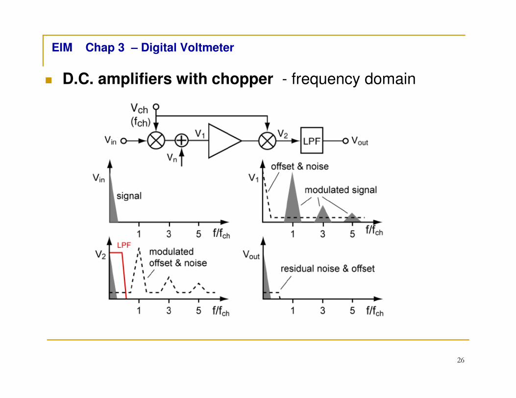
D.C. amplifiers with chopper
Upper way - util voltage: VIN
Lower way - offset voltage VOS (is rejected):
Used for d.c. and a.c. low frequency
Operation: DC → AC conversion (modulation), AC amplifier,
AC → DC conversion (demodulation + LPF)
26
EIM Chap 3 – Digital Voltmeter
D.C. amplifiers with chopper - frequency domain

27
EIM Chap 3 – Digital Voltmeter
D.C. amplifiers with chopper
Variant: rectangular modulation/demodulation signal.
Switch=Z : C2 şi C3 charges with offset voltage
switch=S: C2, C3 voltage compensate offset voltage
R1, C1 = antialiasing LPF
R3, C4 = output LPF

28
EIM Chap 3 – Digital Voltmeter
A.C signal (METc remember)
For u(t)=U sin ωt:
Vmed = 0 (unused)
Vma = Vavg= 2U/π (full-wave rect.) KF = Uef/Uma= π / √2=1.11
Vef = Vrms = U/√2 = 0.707U KV=Uv/Uef = √2
VV = VPK = U
VVV = VPP = VPk-Pk = 2U

29
EIM Chap 3 – Digital Voltmeter
A.C voltmeter types
Obs: All a.c. voltmeter have gradation for sin wave rms
Types:
- a.m. voltmeter gradated in rms value Vrms = Vma · 1.11 (introduce important systematic error for non sin wave signals)
- Peak detector voltmeter gradated in rms value Vrms = Vma · 0.707
- True rms voltmeter – correct indication for all wave forms

30
EIM Chap 3 – Digital Voltmeter
A.C. True rms voltmeter
- thermal effect - thermocouple (slowly, very sensitive of environment factors)
- analog multipliers (ex: Agilent 34405A)
- sampling and digital uP computing (only for repetitive signals)
(ex: Agilent 34410A, TDS 1001
Oscilloscope – measurement menu)

31
EIM Chap 3 – Digital Voltmeter
A.C. voltmeter with D.C. amplifier
Acc
V-metru cc
Det
(conv
ca-cc)
Uin caDIV.
cal.
Detection
(a.c.-d.c convertion)
d.c. voltmeter
d.c.
Amp
Advantages:
High bandwidth (GHz)
Small CIN
Detector : peak, absolute mean, etc;
Disadvantages:
Small RIN
Small sensitivity (x10 mV); nonlinear for small signals
D.C. amplif. gain limited by self noise and thermal leeway

32
Aca
u(t)
V-metru cc
Au(t)
Det
(conv
ca-cc)
DCCUin ca
EIM Chap 3 – Digital Voltmeter
A.C. voltmeter with a.c. amplifier
Detection
(a.c.-d.c convertion)
d.c. voltmeter
a.c.
Amp
Advantages:
high sensitivity (due a.c. amplifier), better linearity;
High RIN , small CIN
Detector : peak, absolute mean, etc;
Disadvantages:
Medium bandwidth (MHz)
DCC must be compensated

33
EIM Chap 3 – Digital Voltmeter
Cabling – two terminal configuration (Hi, Lo)
cm Gs GiE V V= −
voltmeterMeas.
value
dB1 0dBcm
nm
ECMRR CMRR
U= = ⇒ =
nm cmU E=
After passivization, measured valuenE

34
EIM Chap 3 – Digital Voltmeter
Cabling – three wire configuration (Hi, Lo, GND)
Measuring value
Voltmetercm Gs GiE V V= −
1 1 cm b
nm b b
E Z R ZCMRR
U R R
+= = ≅
1
bnm cm
b
RU E
Z R=
+
1 2 1 2,Z Z I I<< >>
Unm on Ra is neglected
Exp: Rb = 1kΩ; Z1 =R1||C1 ( R1=109Ω, C1=2.5 nF )
typically d.c. CMRR = 120dB a.c. (f=50Hz) CMRR = 62dB

35
EIM Chap 3 – Digital Voltmeter
Cabling – three wire configuration (Hi, Lo, GND)
1 2 using , , ,V a b
Z Z Z r r>>
Unm on Ra is neglected
[1]
[0]
[2]
1 2
1
2 1 1
1 2
1 2
1 1 1 1 1 1
1 1 1 1 1 1 1 1
1 1
1 1
a b b a
cm
a V b a V
a b b a
cm cm
a b a V
r r Z r r ZV E
r Z Z r Z r Z Z
r Z r Z r rE E
Z Z
r r r Z
+ − +
=
+ + ⋅ + + + ⋅
−
≅ ≅ − +
2 1
1 2 2
1 2
2 2
1 1 1 1 1 1
1 1 1 1 1
cm cm
a b a a b
cm
a V a a
E EV V
r r Z Z r Z r r
EV V
r Z Z r Z r
+ + + − + = − −
+ + − + =
1
1
nm cm
b
ZU E
Z R=
+

36
EIM Chap 3 – Digital Voltmeter
Cabling - four wire configuration Measuring
valueVoltmeter
cm Gs GiE V V= −
4 4 cm b
nm b b
E Z R ZCMRR
U R R
+= = ≅
4
4
nm cm
b
ZU E
Z R=
+
Exp: Rb = 1kΩ; Z1=R1||C1:( R1=109Ω, C1=2.5 nF ); Z4 : R4=1011 Ω, C4=2.5pF
typically d.c. CMRR = 120dB a.c. (f=50Hz) CMRR = 120dB

37
EIM Chap 3 – Digital Voltmeter
Bibliography S. Ciochina, Masurari electrice si electronice, 1999 ;
ham.elcom.pub.ro/iem;
Application notes - National Instruments;