Chaotic Escape of Photons from a

Fish-Shaped Reflecting Cavity

A thesis submitted in partial fulfillment of the requirement

for the degree of Bachelor of Science with Honors in

Physics from the College of William and Mary in Virginia,

by

Paul C. Hansen

Accepted for

Advisor: Prof. John B. Delos

Prof. Henry Krakauer

Prof. Nahum Zobin

Williamsburg, Virginia

May 2004

Contents

Acknowledgments iv

List of Figures vii

Abstract v

1 Introduction 1

1.1 Background . . . . . . . . . . . . . . . . . . . . . . . . . . . . . . . . 1

1.2 Related Work . . . . . . . . . . . . . . . . . . . . . . . . . . . . . . . 2

2 The System 7

2.1 The Cavity . . . . . . . . . . . . . . . . . . . . . . . . . . . . . . . . 7

2.2 Types of Trajectories . . . . . . . . . . . . . . . . . . . . . . . . . . . 10

2.3 The Phase Plane . . . . . . . . . . . . . . . . . . . . . . . . . . . . . 13

i

2.3.1 The Arc Length Surface Of Section . . . . . . . . . . . . . . . 14

2.3.2 Implications Of Continuity And Uniqueness Of Trajectories . 21

2.3.3 Homoclinic Tangles . . . . . . . . . . . . . . . . . . . . . . . . 22

2.4 Procedure and Description of Results . . . . . . . . . . . . . . . . . . 24

2.4.1 Method . . . . . . . . . . . . . . . . . . . . . . . . . . . . . . 25

2.4.2 Results . . . . . . . . . . . . . . . . . . . . . . . . . . . . . . . 26

3 Homotopic Lobe Dynamics 31

3.0.3 Homotopy Classes . . . . . . . . . . . . . . . . . . . . . . . . 34

3.0.4 The Basis of Path Classes . . . . . . . . . . . . . . . . . . . . 37

3.0.5 Symbolic Representation of Escape . . . . . . . . . . . . . . . 40

3.0.6 Implications . . . . . . . . . . . . . . . . . . . . . . . . . . . . 41

3.0.7 Summary . . . . . . . . . . . . . . . . . . . . . . . . . . . . . 42

4 Results And Analysis 43

4.1 Confirming Epistrophic Structure . . . . . . . . . . . . . . . . . . . . 43

4.2 The Pulse Train . . . . . . . . . . . . . . . . . . . . . . . . . . . . . . 49

ii

5 Conclusions And Future Work 51

Appendix: Implementation Notes 53

5.1 Trajectories . . . . . . . . . . . . . . . . . . . . . . . . . . . . . . . . 53

5.2 Surface Of Section . . . . . . . . . . . . . . . . . . . . . . . . . . . . 56

5.2.1 Tracing The Manifolds . . . . . . . . . . . . . . . . . . . . . . 57

5.2.2 Intersections With E0 . . . . . . . . . . . . . . . . . . . . . . 58

iii

Acknowledgments

Many thanks to...

Kevin Mitchell for helpful mathematical discussions during this project

Hurricane Isabel for sparing my computer and giving me a nice break in the mountains

Prof. Delos, my thoroughly excellent advisor, for being available for consultation

whenever I walked into his office!

S.D.G.

iv

List of Figures

1.1 Time To Escape in Ionization of Hydrogen . . . . . . . . . . . 4

1.2 Fish Cavity . . . . . . . . . . . . . . . . . . . . . . . . . . . . . . . 5

2.1 Hydrogen Potential and Fish Cavity, with e− trajectories . . . . 8

2.2 Neutrally Stable and Stable Orbits . . . . . . . . . . . . . . . . 9

2.3 Unstable Orbits . . . . . . . . . . . . . . . . . . . . . . . . . . . . 9

2.4 The Fish Cavity with parabolic factors . . . . . . . . . . . . . . . . 10

2.5 Initial Ensemble of Trajectories . . . . . . . . . . . . . . . . . . . 11

2.6 Trajectories In The Fish Cavity . . . . . . . . . . . . . . . . . . 12

2.7 Arc Length Coordinates . . . . . . . . . . . . . . . . . . . . . . . 14

2.8 Arc Length Momenta . . . . . . . . . . . . . . . . . . . . . . . . . 15

2.9 Stable and Unstable Orbits in the Phase Plane . . . . . . . . . 16

v

2.10 Reflected Surface of Section . . . . . . . . . . . . . . . . . . . . . 17

2.11 Quasi-Periodic Orbits . . . . . . . . . . . . . . . . . . . . . . . . . 18

2.12 Stable and Unstable Manifolds . . . . . . . . . . . . . . . . . . . 19

2.13 Homoclinic Tangle . . . . . . . . . . . . . . . . . . . . . . . . . . . 20

2.14 Lobes in the Phase Plane . . . . . . . . . . . . . . . . . . . . . . 22

2.15 Phase Portrait of the Fish Cavity System . . . . . . . . . . . . 24

2.16 Line of Initial Conditions . . . . . . . . . . . . . . . . . . . . . . . 26

2.17 Evolution of Line of Initial Conditions . . . . . . . . . . . . . . 27

2.18 Time To Escape superimposed on surface of section . . . . . . . . . 28

2.19 Discrete Escape Time . . . . . . . . . . . . . . . . . . . . . . . . . 29

2.20 Fractal Structure in Time To Escape . . . . . . . . . . . . . . . 30

3.1 Surface of Section . . . . . . . . . . . . . . . . . . . . . . . . . . . 32

3.2 Homoclinic Tangle . . . . . . . . . . . . . . . . . . . . . . . . . . . 34

3.3 Topological Forcing . . . . . . . . . . . . . . . . . . . . . . . . . . 35

3.4 Homotopic Curves . . . . . . . . . . . . . . . . . . . . . . . . . . . 35

3.5 Simple Paths in the Active Region . . . . . . . . . . . . . . . . . 37

vi

3.6 Decomposition of a Curve . . . . . . . . . . . . . . . . . . . . . . 39

4.1 Deriving D = 11 . . . . . . . . . . . . . . . . . . . . . . . . . . . . . 44

4.2 Epistrophic Fractal Time To Escape . . . . . . . . . . . . . . . . 45

4.3 Decomposition of Initial Conditions . . . . . . . . . . . . . . . . 46

4.4 Predicted Escape Segments for M25(L0) . . . . . . . . . . . . . . 48

4.5 Pulse Train . . . . . . . . . . . . . . . . . . . . . . . . . . . . . . . 50

5.1 Choosing Cutoff Point . . . . . . . . . . . . . . . . . . . . . . . . 56

vii

Abstract

We consider the escape of a microwave photon or a particle bouncing ballistically

from an open, fish-shaped reflective cavity. Trajectories within the cavity may be

chaotic, regular or periodic, so not all initial conditions lead to escape. Rather, if

we fix the initial position of the photon and record escape time as a function of

the initial direction, the resulting escape-time diagram shows “epistrophic fractal”

structure—repeated structure within structure at all levels of resolution, with new

features introduced into the fractal at longer time scales. At an external detector an

observer would note a characteristic pulse train of escaping particles. We approach

the problem through simulation using Matlab, but the setup is simple and lends itself

to verification in the laboratory.

Chapter 1

Introduction

1.1 Background

We study a system involving “chaotic escape”—the system is open, so trajectories may

enter and leave, but the amount of time spent within the system is a highly-sensitive

function of initial conditions. Nearby trajectories diverge exponentially over time, so

it is effectively impossible to predict behavior of specific trajectories over long time

scales. However, governing principles exist which qualitatively and quantitatively

describe the behavior of sets of trajectories. Some of these principles have been known

for years: for example, scientists have known for several decades that chaotic systems

often exhibit fractal structure in various ways (a fractal is a figure with self-similar

features at all levels of resolution). Well known fractals show regular self-similarity

(e.g. the Cantor set), asymptotic self-similarity (e.g. sequences of period-doubling

bifurcations) or statistical self-similarity (e.g. coastlines and clouds) [3]. But under

certain circumstances, a chaotic system may exhibit a fourth type of fractal structure

1

called epistrophic self-similarity. Kevin Mitchell of William and Mary has recently

developed a quantitative interpretive structure for these epistrophic fractals, known as

homotopic lobe dynamics, which explains much but not all of the observed structure

[4]. The present system was chosen to meet the criteria for epistrophic self-similarity

(to be listed later) and provides a test case for application of Mitchells mathematics.

1.2 Related Work

Tiyapan and Jaffe [6] analyzed a chaotic scattering system in the early 1990s. In the

scattering of He from I2, depending on its intial position and momentum the helium

atom may be temporarily trapped in a potential well around the iodine. The initial

angle-final action plot is smooth for most initial angles but assumes a very complicated

structure for a small set of angles. Within this chaotic region, contiguous segments

of initial angles map smoothly to the final action, but in between these segments

the final action varies wildly (Miller uses the term “chattering trajectories”). The

smooth segments of initial conditions, called icicles for their pointed appearance,

form patterns that repeat at all scales. Tiyapan and Jaffe examined these patterns at

seven levels of resolution and gave evidence of asymptotic self-similarity between the

icicles each level. Groups of icicles form a convergent infinite series which Mitchell et

al. call an epistrophe.

Recently, analogous phenomena in the escape of high-Rydberg electrons from hydro-

gen atoms in parallel electric and magnetic fields have been found [5]. This system is

one of the simplest possible that allows chaos. The motion of a highly-excited elec-

tron near a proton is well understood from classical mechanics, and is not chaotic: the

2

proton creates a potential well and the electron moves in an elliptical, parabolic or

hyperbolic trajectory depending on its energy. Under application of a constant elec-

tric field, the electrons orbits stretch, and for a strong enough field even the tightly

bound orbits will be ripped from the proton. In this case, the equations of motion

are separable, and the trajectories remain regular. The application of a magnetic

field couples the degrees of freedom: the magnetic force F = qV × B accelerates the

electron perpendicularly and brings on chaotic dynamics. Under parallel electric and

magnetic fields, the spherical inverse-square potential well is deformed into a teardrop

shape, roughly centered at the proton but pinching into a saddle point downstream

in the electric field. Electrons may only escape by crossing this saddle point. Unlike

the zero-field case, energy alone does not determine whether an electron is bound or

unbound—rather, the time taken for an excited electron to escape over the saddle

region depends sensitively on the combination of initial position and velocity. Two

electrons of equal energy, starting on only slightly different trajectories, may escape

at very different times; one may escape early while the other remains trapped in wild

orbits around the proton forever.

Mitchell simulated sets of trajectories of equal energy and studied the relationship

between initial angle and time to escape. Trajectories which head straight for the

saddle point may escape very quickly, but if they aim too far to the side they will

oscillate laterally and fail to cross the saddle, eventually falling back into the well and

winding around the proton again. The set of intial angles leading to quick escape form

an “escape segment in Mitchell’s plot. Sets of nearby initial conditions that orbit the

proton once before escape form secondary escape segments; in fact, the segments en

of the initial angular distribution which escape in n transverse oscillations form an

infinite series, each segment growing exponentially narrower. We can see structure-

3

within-structure in this escape-time plot, and on closer examination we would find

infinite sequences which display asymptotic self-similarity.

Figure 1.1: Time To Escape in Ionization of Hydrogen

These escape segments are only the first of many layers of order in the escape-time

plot. However at longer times there appear “unexpected” escape segments which

Mitchell et al. call “strophes.” These strophes break the pattern of earlier escape

segments. At very long time scales, the strophes come to dominate the fractal. Such

epistrophic fractals, developing new order at high levels of resolution, appear in many

chaotic systems. We see hints of this behavior in Figure 1.1, and we will give examples

from our system later.

Mitchell found a mathematical way to predict epistrophes by examining the phase

plane—the plot of a single coordinate and its related momentum. The resulting

“homotopic lobe dynamics” is applicable to many chaotic systems, provided that they

satisfy certain criteria (given in [3], [4]). The short-time behavior of the hydrogen

4

system is fully described by Mitchells method, but the unexpected strophic escape

segments are not yet fully accounted for.

Over the summer of 2003, REU student Melissa Commisso began work on the present

project, simulating the escape of photons from a fish-shaped reflective cavity (Fig-

ure 1.2) [1]. This system was conceived as a more lab-friendly alternative to the

hydrogen ionization experiments—it features similar dynamics and produces anal-

ogous escape-time fractals, but the physical experiments may be performed using

microwaves in two dimensions on a lab table. Commisso used Maple to model the

cavity and trajectories, and produced escape-time plots showing escape segments and

structure within structure. Unfortunately Maple proved to be an inadequate tool for

such programmatic tasks and hindered progress substantially.

Figure 1.2: Fish Cavity

Beginning in Fall 2003, we rewrote the simulator using Matlab and carried out nu-

5

merical experiments similar to Mitchell’s hydrogen simulations. In Chapter 2 of this

paper we give a physical overview of the system, including the choice of the cavity

shape and possible resulting trajectories. Then we give a primer on dynamics in the

phase plane and a qualitative overview of the results, particularly the epistrophic

fractal structure in the escape-time plot and resulting characteristics of the outgoing

pulse train. Chapter 3 is solely devoted to homotopic lobe dynamics, and Chapter

4 applies those techniques to our phase plane to explain our escape-time plots and

predict features at all levels of resolution. The appendix presents technical details of

our implementation.

6

Chapter 2

The System

2.1 The Cavity

The shape of a reflecting cavity determines the types of trajectories that may propa-

gate inside it. Practically speaking, a cavity that superficially resembles the hydrogen

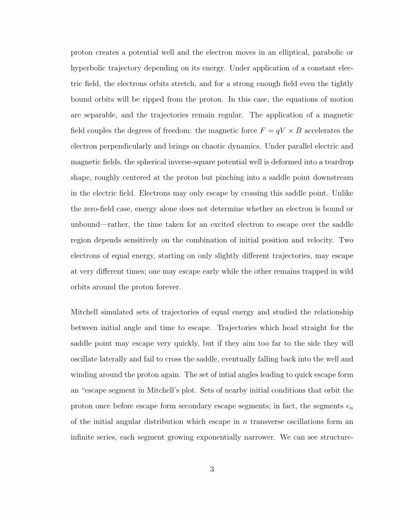
saddle potential supports similar chaotic dynamics (Figure 2.1). In the hydrogen sys-

tem, an electron may be trapped in a stable region in which it orbits the proton for

all time. The reflecting cavity must provide a similar stable region in which photons

may bounce back and forth without escape. Electrons may only escape the hydrogen

system by passing the saddle point, and if they fail to cross they will turn slowly

and return for another orbit in the well. Likewise, the reflecting cavity must have a

bottleneck that allows escape for certain trajectories but turns back trajectories with

too much transverse motion. Electrons that cross the saddle point in the hydrogen

system never return; the outside of the reflecting cavity must flare to prevent escaped

photons from returning before reaching an external detector. Lastly, the cavity must

7

be relatively smooth to minimize discontinuities in the dynamics—nearby trajectories

can diverge over a sequence of bounces but they should not be abruptly split apart

by cusps or corners. Our system does feature one discontinuity associated with the

curvature in the narrow region, but in the present case this does not complicate the

dynamics.

Figure 2.1: Hydrogen Potential and Fish Cavity, with e− trajectories

Let us think about stability and instability of orbits. Consider a two-dimensional

circular cavity. A photon released on a diameter of this circle will remain on that

diameter forever, bouncing back and forth (Figure 2.2). However under slight per-

turbations of the initial angle, the photon will precess around the entire circle at a

constant rate. This is known as neutral stability—nearby trajectories move apart lin-

early in time. However, if two pieces were cut from the circle and the remaining arcs

were brought together, trajectories between the two walls would be stably confined

forever. On the other hand, were the two arcs separated by more than the original

8

diameter, trajectories would be unstable and escape.

Figure 2.2: Neutrally Stable and Stable Orbits

Consider also a pair of facing convex surfaces (Figure 2.3). Classically a photon could

bounce ballistically between the extrema of these surfaces forever. However, this orbit

is unstable—if perturbed, it will exponentially diverge from the transverse orbit.

Figure 2.3: Unstable Orbits

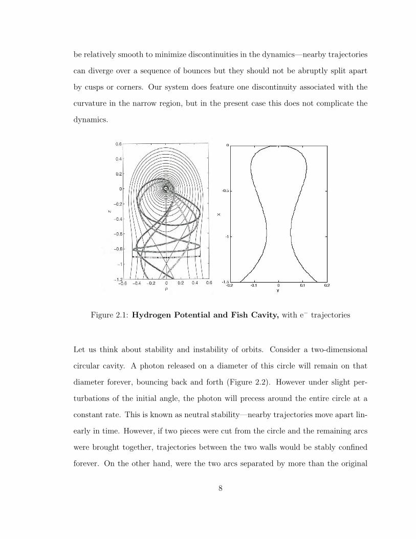
To combine these unstable and stable regions into one surface, we compose several

parabolic sections (Figure 2.1). The first, forming the nose of the fish, faces outward

along the x-axis. Further along the positive x-axis we create a hyperbolic-like bottle-

neck by pairing two parabolas oriented outwards in the y-direction (Figure 2.4). We

multiply the parabolas to combine them into one surface. The shape can be further

fine-tuned by adjustment of three parameters: A, the steepness of the bottleneck;

w, the width of the bottleneck region; and L, the position of the bottleneck on the

x-axis. Practically speaking, A is the means to adjust the height of the cavity, and

modifying A is sufficient to alter the systems dynamics. Early on we set L = 1 and

9

w = 0.2 (in arbitrary units); we have not changed them since.

y = f(x) = ±√

x(w

2+ A(x− L)2

)(2.1)

0 0.5 1 1.5-0.4

-0.3

-0.2

-0.1

0

0.1

0.2

0.3

0.4

x

y

Figure 2.4: The Fish Cavity with parabolic factors

We position a simulated “detector” at x = 1.5, well outside the bottleneck. In the

simulation it is sufficent to say that this is where trajectories end. In the lab, this

could be an absorbing boundary, or one might put a small microwave detector at

various points along this boundary.

2.2 Types of Trajectories

We release an ensemble of trajectories from a point on the wall of the cavity, rep-

resenting the wavefront of a microwave burst. We graph such a set of trajectories

10

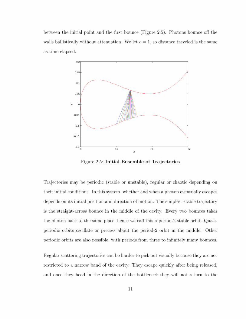
between the initial point and the first bounce (Figure 2.5). Photons bounce off the

walls ballistically without attenuation. We let c = 1, so distance traveled is the same

as time elapsed.

0 0.5 1 1.5-0.2

-0.15

-0.1

-0.05

0

0.05

0.1

0.15

0.2

X

Y

Figure 2.5: Initial Ensemble of Trajectories

Trajectories may be periodic (stable or unstable), regular or chaotic depending on

their initial conditions. In this system, whether and when a photon eventually escapes

depends on its initial position and direction of motion. The simplest stable trajectory

is the straight-across bounce in the middle of the cavity. Every two bounces takes

the photon back to the same place, hence we call this a period-2 stable orbit. Quasi-

periodic orbits oscillate or precess about the period-2 orbit in the middle. Other

periodic orbits are also possible, with periods from three to infinitely many bounces.

Regular scattering trajectories can be harder to pick out visually because they are not

restricted to a narrow band of the cavity. They escape quickly after being released,

and once they head in the direction of the bottleneck they will not return to the

11

cavity. The most recognizable regular trajectories are the whispering gallery modes

which stay close to the wall of the convex region before escaping. None of the regular

trajectories are particularly interesting and we usually omit as many of them as

possible from our initial ensembles.

The chaotic trajectories occupy the region between regular scattering and stable tra-

jectories. Photons that approach the bottleneck several times before finally escaping

follow chaotic trajectories. A chaotic orbit may remain in the cavity forever without

once repeating its position and velocity. As with the hydrogen system, the escape-

time plot for a set of chaotic trajectories forms an epistrophic fractal.

Examples of stable, unstable and regular scattering trajectories are shown in Figure

2.6.

0 0.5 1 1.5-0.2

-0.15

-0.1

-0.05

0

0.05

0.1

0.15

0.2

x

y

Unstable Orbit

Regular Scattering (Whispering Gallery) Orbit

Stable Orbit

Figure 2.6: Trajectories In The Fish Cavity

Let us consider continuity and uniqueness of trajectories. The methods of homotopic

12

lobe dynamics assume that the system can be modeled by an continuous area- and

orientation- preserving saddle-center map. Among other things, this means that

continuously changing a trajectory’s initial conditions will continuously change all its

future positions and velocities. If a photon begins at (x0, v0) and next bounces to

(x1, v1), a smooth change in (x0, v0) should never result in a discontinuous jump in

(x1, v1). There is in fact a possible discontinuity, due to concavity in the bottleneck

region, where the transition between trajectories from inside that brush the bottleneck

and escape directly to the detector is abrupt. Fortunately this discontinuity does not

affect dynamics inside the cavity.

Uniqueness of trajectories means that if two trajectories are ever at the same point

with the same velocity, they will continue to be the same for all time (past and

future). The combination of uniqueness and continuity permits powerful topological

arguments about ordering of trajectories in the future.

2.3 The Phase Plane

All the defining characteristics of the cavity and trajectories within it may be un-

derstood in the phase plane. For a system with two degrees of freedom, it may be

sufficient to focus on just one generalized coordinate and its associated momentum.

We found that the best coordinate and momentum in our system are the distance l

along the wall where each bounce occurs and the momentum pl parallel to the wall at

that bounce. For every bounce we plot l and pl; a single trajectory will form a series

of dots on this surface of section. By this method we uncover essential features of the

system that are difficult to see by watching trajectories propagate in the cavity, such

13

as stable and unstable regions of the phase plane, stable fixed points and periodic

orbits, stable and unstable manifolds of unstable fixed points, and regions of chaos.

These terms will be introduced by examples from the fish-cavity system. In fact the

simple ideas of continuity and uniqueness of trajectories in the cavity are corollaries

of deeper ideas in the phase plane, often related to ideas from ordinary differential

equations.

2.3.1 The Arc Length Surface Of Section

Assign to each point on the cavity wall a coordinate l equal to the clockwise distance

from the origin (the nose of the fish) (Figure 2.7). When a photon strikes the wall its

associated momentum pl is the component of its velocity vector parallel to the wall

(recall p = v = c = 1 in simulation units). A regular whispering gallery trajectory

maintains a large (nearly 1.0 or -1.0) pl along the interior of the cavity (Figure 2.8).

0 0.2 0.4 0.6 0.8 1 1.2 1.4 1.6-0.2

-0.15

-0.1

-0.05

0

0.05

0.1

0.15

0.2

x

l = 0

l = 0.3l = 0.6

l = 0.9 l = 1.2

l = 1.5

l = -1.5

l = -1.2l = -0.9l = -0.6

l = -0.3

†

pl > 0

†

pl < 0

Figure 2.7: Arc Length Coordinates

The trajectory in Figure 2.6 is confined to the top wall of the cavity where l > 0.

As a result its trace in the phase plane remains on the right of the origin. However

most trajectories leave traces alternating between l < 0 and l > 0. Consider an

14

0 0.5 1 1.5-0.2

-0.15

-0.1

-0.05

0

0.05

0.1

0.15

0.2

X

†

pl = 0.98

†

pl = 0.0†

pl = -0.98

Figure 2.8: Arc Length Momenta

orbit released in the bottleneck region, drifting left into the cavity (Figure 2.9). Its

cartesian momentum px is negative at each bounce, but pl is positive for bounces at

the bottom of the cavity (l < 0) and negative for bounces at the top (l > 0). Points

on the surface of section thus alternate between the second and fourth quadrants.

Likewise the primary stable and unstable period-2 orbits alternate between the left

and right sides of the surface of section, with pl = 0.

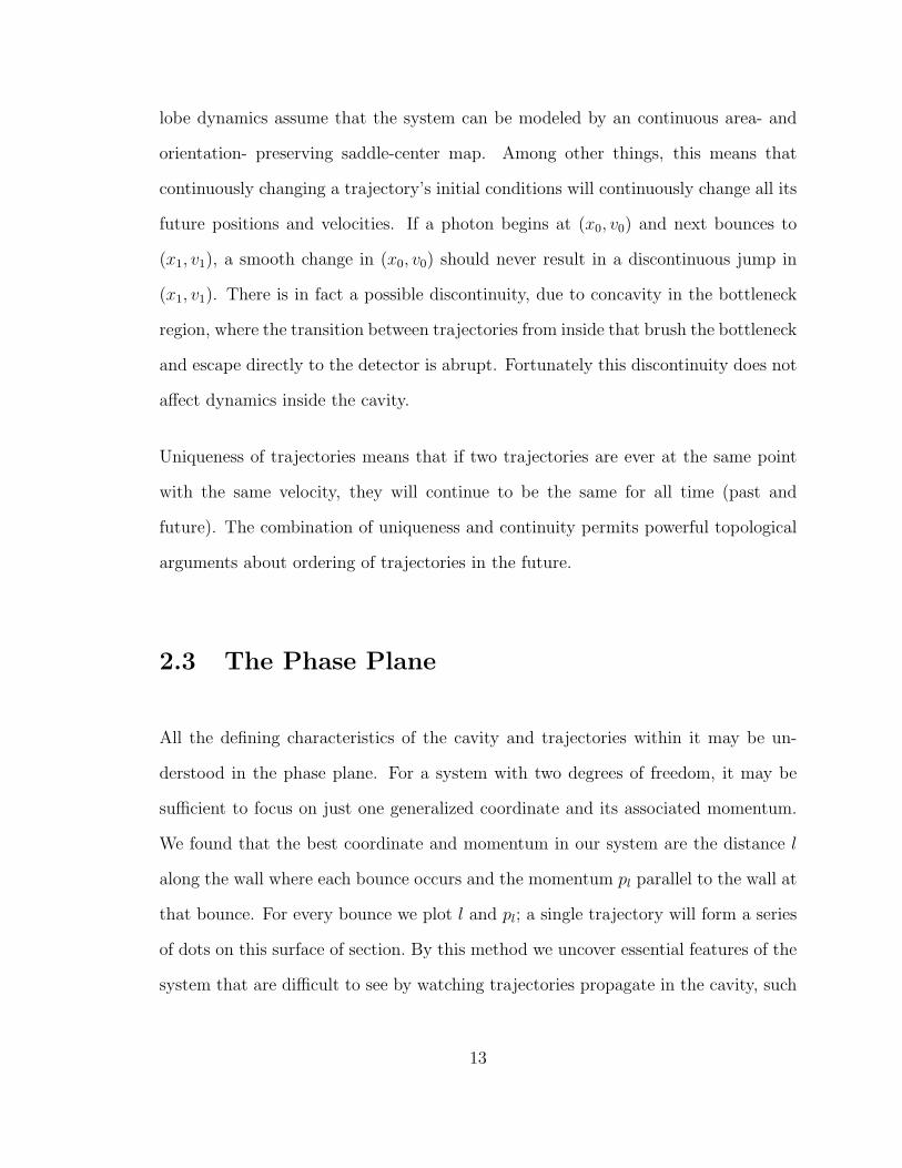
Let us introduce a simplification to take advantage of the fish curves reflection symme-

try in y. In the original surface of section, the orbits in Figure 2.9 leave symmetric or

quasi-symmetric paths; the natural odd-symmetry suggests that all points (l < 0, pl)

be reflected through the origin. Suppose we place a reflecting boundary on the x-axis

(y = 0). Then any orbit which would have gone from the top of the fish (l0 > 0)

to the bottom of the fish (l1 < 0) is actually reflected to the point (−l1 > 0,−pl1).

Therefore when we run the map (l0, pl0) → (l1, pl1), we may add a condition: if l1 < 0,

then replace (l1, pl1) by (−l1,−pl1). In the new surface of section a stable period-2

orbit looks like a single point, and any other orbit traces a single succession of points

in the phase plane (Figure 2.10).

15

0 0.5 1 1.5-0.2

-0.1

0

0.1

0.2Trajectories

x

-1 -0.8 -0.6 -0.4 -0.2 0 0.2 0.4 0.6 0.8 1-1

-0.5

0

0.5

1

l

Surface Of Section

Figure 2.9: Stable and Unstable Orbits in the Phase Plane

This reflected surface of section retains all the information of the old one. True,

there is no longer a distinction between a bounce on the bottom of the curve and

a bounce on the top. However, it has already been shown that these situations are

effectively identical: the mapping between reflecting pairs of trajectories and paths in

the surface of section is still one-to-one. The simplified mapping is now easily lined

up with the diagram of the fish cavity (as in Figure 2.11). The phase plane provides

the best means to analyze nonlinear systems and retains all the information from the

cavity diagrams, hence from now on we shall study events in phase plane rather than

events in the cavity.

The orbits in the cavity induce a map M on the surface of section. The map converts

photon position and velocity at one bounce to new position and velocity at the next

bounce in the cavity. Five iterates of the map trace a five-bounce trajectory from one

initial condition. M is a map from the phase plane to itself, so we may plot the evo-

16

0 0.5 1 1.5-0.2

-0.1

0

0.1

0.2Trajectories

x

0 0.2 0.4 0.6 0.8 1 1.2 1.4 1.6-1

-0.5

0

0.5

1Surface Of Section

l

Figure 2.10: Reflected Surface of Section

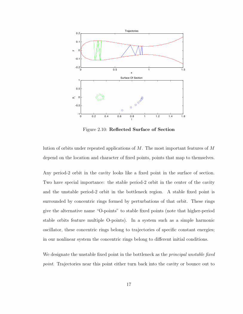
lution of orbits under repeated applications of M . The most important features of M

depend on the location and character of fixed points, points that map to themselves.

Any period-2 orbit in the cavity looks like a fixed point in the surface of section.

Two have special importance: the stable period-2 orbit in the center of the cavity

and the unstable period-2 orbit in the bottleneck region. A stable fixed point is

surrounded by concentric rings formed by perturbations of that orbit. These rings

give the alternative name “O-points” to stable fixed points (note that higher-period

stable orbits feature multiple O-points). In a system such as a simple harmonic

oscillator, these concentric rings belong to trajectories of specific constant energies;

in our nonlinear system the concentric rings belong to different initial conditions.

We designate the unstable fixed point in the bottleneck as the principal unstable fixed

point. Trajectories near this point either turn back into the cavity or bounce out to

17

0 0.5 1 1.5-0.2

-0.1

0

0.1

0.2Example Quasi-Periodic Trajectory

X

0 0.2 0.4 0.6 0.8 1 1.2 1.4 1.6-1

-0.5

0

0.5

1Surface of Section: Family of Quasi-Periodic Orbits

l

Figure 2.11: Quasi-Periodic Orbits

the detector, so there are no concentric rings as around a stable fixed point. Rather,

orbits near an unstable fixed point accelerate outwards in opposite directions along a

line in the surface of section. This line is called the unstable manifold (alternatively,

out-set) of the unstable fixed point. Similarly, the stable manifold (alternatively,

in-set) is the set of all trajectories that map into the unstable fixed point. Due

to symmetry in the fish curve, the stable manifold is the reflection of the unstable

manifold with pl → −pl. The manifolds meet transversely at the unstable fixed point,

marking it as an X-point. We graph portions of the two manifolds in Figure 2.12.

Every point on the stable or unstable manifold continues to map onto that manifold for

all time. This includes the homoclinic points marking intersections between the stable

and unstable manifolds. One may easily prove that the existence of one homoclinic

point implies the existence of an infinity of homoclinic points converging on the X-

point along both manifolds. Hence the manifolds cross and re-cross infinitely many

18

0 0.2 0.4 0.6 0.8 1 1.2 1.4 1.6-1

-0.8

-0.6

-0.4

-0.2

0

0.2

0.4

0.6

0.8

1Surface of Section, (l,pl), 42 bounces

l

Principal Intersection Point Unstable Fixed Point

Unstable Manifold

Stable Manifold

Figure 2.12: Stable and Unstable Manifolds

times in a wildly complicated homoclinic tangle (Figure 2.13). Going forward in

time, each homoclinic point maps towards the X-point along the stable manifold;

going backward in time, the pre-images of each homoclinic point converge towards

the X-point along the unstable manifold.

How can an infinity of homoclinic points fit onto the finite segments of both manifolds

from the unstable fixed point to the principal homoclinic point, if chaotic trajectories

diverge exponentially? We make a comparison to a simple system of differential

equations: linearize the map M , connecting it to an iterative solution to a pair

of linear ordinary differential equations. The two eigenvectors lie parallel to the

stable and unstable manifolds; the eigenvalues are the rates of exponential divergence

outward along those directions. Hence the unstable manifold must attract nearby

trajectories, and the stable manifold must repel nearby trajectories (under time-

reversal the opposite holds).

19

0 0.2 0.4 0.6 0.8 1 1.2 1.4 1.6-1

-0.8

-0.6

-0.4

-0.2

0

0.2

0.4

0.6

0.8

1Poincare Surface of Section, (l,pl) Coordinates

l

Figure 2.13: Homoclinic Tangle

Now consider a set of initial conditions surrounding the X-point. As they map forward

they converge upon the unstable manifold and accelerate exponentially along it. At

each mapping, the set of trajectories distorts along the unstable manifold, lengthening

and narrowing proportionally to the eigenvalues of the map at the X-point. As will be

discussed shortly, the map preserves area, and it follows that the two eigenvalues are

reciprocals of each other. The larger of the two eigenvalues, the Liapunov exponent of

the principal unstable fixed point, determines the rates of convergence and divergence

of trajectories in the phase plane.

20

2.3.2 Implications Of Continuity And Uniqueness Of Trajec-

tories

By the one-to-one mapping of cavity trajectories to phase plane trajectories, conti-

nuity and uniqueness of trajectories now becomes continuity of the map and unique-

ness of trajectories on the surface of section. Uniqueness of trajectories is already

obvious—the simulator map M cannot assign two images to one point in the phase

plane. Actually we can safely extend uniqueness to entire stable and unstable mani-

folds made of an infinity of trajectories: neither the stable nor the unstable manifold

can cross itself. Continuity of the orbits, together with certain properties of Hamil-

tonian dynamical systems, implies that M is a continuous area- and orientation-

preserving map on the phase plane (except in escape regions).

• Continuous: M preserves properties of sets. Connected sets remain connected;

points map to points, curves map to curves, connected regions map to connected

regions.

• Area-preserving: the measure of a connected set will remain constant under M .

Shapes can deform but areas will be preserved. This is proven in the linearized

area near an unstable fixed point by equality of eigenvalues, but is also true in

the entire phase plane. There is one exception to the rule: after escaping from

the cavity the point maps to infinity. Then area preservation is meaningless.

• Orientation-preserving: a right-handed intersection of two directed curves maps

to another right-handed intersection of two directed curves.

We may apply these properties to entire lobes bounded by the stable and unstable

manifolds (Figure 2.14). Because the manifolds cross at alternate right- and left-

21

handed homoclinic points, orientation preservation implies that each homoclinic point

maps to its second neighbor: there are two infinite interlaced sequences of homoclinic

points. These alternating points bound two sets of lobes that map into themselves;

by area preservation the lobes must have equal areas as long as none of the points

maps to infinity.

†

E0†

E1

†

E2

†

E3

†

E4

†

E5

†

C0

†

C1

†

C2

†

C3

†

C4

†

C5

†

C-1

†

C-2

†

C-3

†

C-4

†

C-5

†

E-1

†

E-2

†

E-3

†

E-4

†

E-5

M

M

Figure 2.14: Lobes in the Phase Plane

2.3.3 Homoclinic Tangles

Henri Poincare discovered the properties of homoclinic tangles over one-hundred years

ago; Chapter 3 introduces the newer homotopic lobe dynamics for describing these

22

tangles. In the meantime several more features the map deserve attention: island

chains, discontinuities in the escape region, and the region of regular trajectories.

A relatively complete phase portrait of the system (Figure 2.15 includes a sequence

of independent O-points bounds the stable region. The center of each island belongs

to the same trajectory, in this case period-10. Orbits slightly displaced from this

period-10 stable orbit map out sets of concentric rings around the O-points: the

first ring around each of the ten O-points belongs to one trajectory. An X-point

lies between each pair of adjacent O-points in the island chain, with its own stable

and unstable manifolds. When the manifolds of separate X-points cross, they form

small heteroclinic tangles of infinite complexity, which sometimes interact with the

tangle of the principal unstable fixed point. Island chains often are present in the

boundary region between stability and chaos, and they cause increased complexity of

escape-time plots.

As already mentioned, if a trajectory escapes from the cavity, it may go to infinity

with no further bounces. In this case the area-preservation in the map becomes

meaningless. Indeed the escaping lobes do not share the same area. As will be

discussed in depth later, these lobes are regions from which trajectories may escape

to the detector in one bounce. Fortunately any lobe which does not lose trajectories

will map to a lobe of the same area.

The entire region outside the stable and unstable manifolds is the domain of regular

scattering trajectories. These trajectories tend to escape in a short time. If a simu-

lation includes a lot of regular trajectories they will dominate the early part of the

escape-time diagram; the behavior featuring fractal structure begins after the regular

trajectories have all escaped. Usually the regular initial conditions are omitted from

23

0 0.2 0.4 0.6 0.8 1 1.2 1.4 1.6-1

-0.8

-0.6

-0.4

-0.2

0

0.2

0.4

0.6

0.8

1SOS, abs(l), pl

l

Figure 2.15: Phase Portrait of the Fish Cavity System

our runs for this reason.

2.4 Procedure and Description of Results

With the prerequisite information and mathematics in place, we present the basic

calculation and results, deferring full analysis to Chapter 4. We show that the system

is analogous to the hydrogen system in its essential features: time to escape plotted

as a function of initial pl includes escape segments organized into infinite converging

sequences called epistrophes; epistrophes spawn new epistrophes at all levels of reso-

lution; unexpected new escape segments called strophes appear at longer times and

spawn epistrophes of their own. The escape segments thus comprise an epistrophic

fractal. The geometric rate of shrinking of escape segments notably asymptotes to the

24

Liapunov exponent of the principal unstable fixed point, suggesting that this fractal

structure is intimately linked to the infinite converging sequences of homoclinic points

on the stable and unstable manifolds.

2.4.1 Method

Select a vertical line of initial conditions L0 in the phase plane, between (l0, pl0)

and (l0,−pl0) where l0 < lunstable. This specifies an outgoing wavefront from a single

emission point on the cavity wall. Photons propagate in all directions from this point,

from nearly parallel to the wall (pl = ±1.0) to normal to the wall (pl = 0). Sample

the line of initial conditions by choosing N uniformly distributed points in the phase

plane from (l0,−pl0) to (l0, pl0)1. As an example, a line of twenty-five initial points

is shown below in the phase plane, with its accompanying initial trajectories in the

cavity (Figure 2.16). (We plot portions of the stable and unstable manifolds for

reference).

Of note: the initial conditions near the middle of L0 intersect the stable zone and map

within the cavity forever as stable orbits. Other initial conditions within the bounds

of the two manifolds begin chaotic trajectories which escape in various amounts of

time, sensitively dependent on the exact initial velocity. Many initial conditions are

outside the stable and unstable manifolds, with |pl| & 0.6. These represent regular

scattering trajectories, and they escape quickly, e.g. around the wall of the cavity in

whispering gallery modes.

Let us represent the trajectories in the phase plane one bounce at a time. The line of

1Uniformity is convenient but not essential to the results.

25

0 0.5 1 1.5-0.2

-0.1

0

0.1

0.2Trajectory Plot

X

0 0.2 0.4 0.6 0.8 1 1.2 1.4 1.6-1

-0.5

0

0.5

1

l

Figure 2.16: Line of Initial Conditions

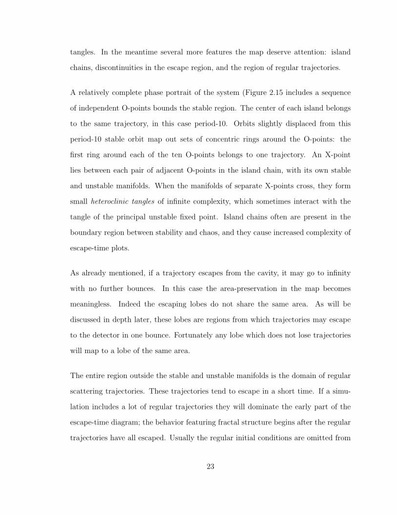
initial conditions maps into a curve, rotated clockwise and sheared in the phase plane

(Figure 2.17). We continue this until most of the trajectories escape, then plot each

photons time to reach the detector (or distance traveled) as a function of its initial

momentum pl0. The result for 1000 photons after forty bounces is shown in Figure

2.18.

2.4.2 Results

The time to escape is jagged, with many singularities. Certain points along the

line of initial conditions are local minima of the time to escape: these minima mark

the centers of icicles in the escape time plot, as observed by Tiyapan and Jaffe and

Mitchell. The central stable segment leaves a hole in the plot.

In the laboratory it is most natural to measure a photon’s time to escape, but for

26

0 0.2 0.4 0.6 0.8 1 1.2 1.4 1.6-1

-0.8

-0.6

-0.4

-0.2

0

0.2

0.4

0.6

0.8

1

l

†

L0

†

M L0( )

†

M2 L0( )

†

M 3 L0( )

†

M 4 L0( )

Figure 2.17: Evolution of Line of Initial Conditions

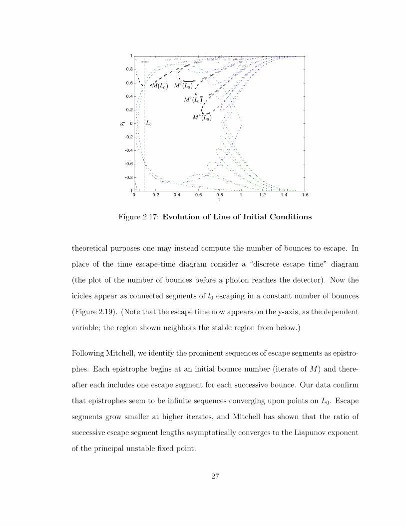
theoretical purposes one may instead compute the number of bounces to escape. In

place of the time escape-time diagram consider a “discrete escape time” diagram

(the plot of the number of bounces before a photon reaches the detector). Now the

icicles appear as connected segments of l0 escaping in a constant number of bounces

(Figure 2.19). (Note that the escape time now appears on the y-axis, as the dependent

variable; the region shown neighbors the stable region from below.)

Following Mitchell, we identify the prominent sequences of escape segments as epistro-

phes. Each epistrophe begins at an initial bounce number (iterate of M) and there-

after each includes one escape segment for each successive bounce. Our data confirm

that epistrophes seem to be infinite sequences converging upon points on L0. Escape

segments grow smaller at higher iterates, and Mitchell has shown that the ratio of

successive escape segment lengths asymptotically converges to the Liapunov exponent

of the principal unstable fixed point.

27

0 1 2 3 4 5 6 7 8-1

-0.8

-0.6

-0.4

-0.2

0

0.2

0.4

0.6

0.8

1

time to escape†

Ï

Ì Ô Ô

Ó Ô Ô

†

Ï

Ì

Ô Ô

Ó

Ô Ô

†

Ï

Ì

Ô Ô

Ó

Ô Ô

†

Ï

Ì Ô Ô

Ó Ô Ô

†

Ï

Ì Ô Ô

Ó Ô Ô

Stable Region

Chaotic Region

Chaotic Region

RegularScatteringRegion

RegularScatteringRegion

Figure 2.18: Time To Escape superimposed on surface of section

More epistrophes appear at higher iterates in the discrete time plot, featuring smaller

initial (and subsequent) escape segments with the same properties as the main epistro-

phe. These new sequences converge on the endpoints of each escape segment in the

first epistrophe; in general and for all time, two epistrophes appear and flank each

escape segment delta iterates later. For this system ∆ = 12. We discuss this “epistro-

phe start rule” later.

This combination of rules imposes fractal order on the escape-time diagram: repeated

structure within structure at all levels of resolution. Figure 2.20 compares sections

of the escape time plot at successive levels of resolution in pl0: the features at larger

scales repeat at smaller scales. New features also appear at some levels of resolution,

escape segments that are not connected to larger-scale structure. These new icicles

spawn epistrophes of their own but are not members of any previous epistrophes. We

mark one of these “strophes” with an asterisk.

28

-0.56 -0.54 -0.52 -0.5 -0.48 -0.46 -0.440

5

10

15

20

25

30

35

40

pl0

Figure 2.19: Discrete Escape Time

Such epistrophic fractals appear in many physical systems including ionization of

hydrogen in parallel electric and magnetic fields. Open chaotic systems satisfying a

few requirements may possess the necessary homoclinic tangle to force such fractal

structure. Chapter 3 presents homotopic lobe dynamics to partially explain and

predict this structure; we apply it to our system in Chapter 4.

29

-0.56 -0.54 -0.52 -0.5 -0.48 -0.46 -0.440

5

10

15

20

25

30

-0.495 -0.494 -0.493 -0.492 -0.491 -0.49 -0.489 -0.488 -0.4870

5

10

15

20

25

30

-0.4907 -0.4906 -0.4905 -0.4904 -0.4903 -0.4902 -0.49010

5

10

15

20

25

30

pl0

*

Figure 2.20: Fractal Structure in Time To Escape

30

Chapter 3

Homotopic Lobe Dynamics

We now provide the mathematics to explain the escape-time diagram by analysis of

the surface of section. Homotopic lobe dynamics reduces the evolution of a curve in

phase space to the evolution of an associated symbol sequence. Following Mitchell’s

method in [4] we use this model to prove the existence of a minimal required set

of escape segments, describe a simple algorithm to generate this set, and show how

recursion in this algorithm explains the spawning of new epistrophes near escape

segments. The symbolic dynamics requires the introduction of new terminology for

regions of the surface of section, whence we begin.

Consider a simple homoclinic tangle (Figure 3.1)1. The stable and unstable mani-

folds bound and define an invariant region of the phase plane, the active region: by

continuity and orientation preservation, M maps all the points in the invariant region

back into the region, and points outside the region (regular scattering trajectories)

never enter it. The trajectories of interest all lie inside the active region. The middle

1Figures in this chapter are adapted from Mitchell [4].

31

of the active region, bounded on top by the stable manifold and below by the unsta-

ble manifold, is the complex. All bound trajectories stay in the complex, but many

escape. A series of successive capture zones map into the complex from below the

unstable manifold, and a mirror-image sequence of escape zones leave the complex

above the stable manifold. Orbits only leave the complex through the escape zones,

and only enter through the capture zones. Orbits that leave the complex may never

return, hence we redefine escape as exiting the complex through escape zone E0.

Active Region

Complex

Stable Manifold

Unstable Manifold

Principal Intersection X-Point

E-1

E0E1

C-1C0

C1

H-1

H0 H1

H-2 H-3

Figure 3.1: Surface of Section

The tangle inside the complex forces intersections of capture and escape zones which

facilitate transport through the complex. All of the area that maps into the complex

via zones C−1, C0, C1 etc. sooner or later escapes through zones E−1, E0, E1 etc. The

escape zones and capture zones intersect an infinite number of times, and as there is

an infinity of escape zones in the complex (pre-images of E0), there is no upper bound

on the number of iterates that a trajectory may spend between C0 and E0. There

is however a lower bound—the minimum number of iterates a scattering trajectory

32

may spend in the complex depends on the first intersection E−n ∩ Cn, dependent on

the topology of the complex. We call this the minimum delay time, D:

D = 2n− 1 (3.1)

In Figure 3.1, capture zone C1 intersects escape zone E−1 in a shaded region H. Thus

D = 1: all pre-images M−n(H) lie in capture zones C0, C−1, ... outside the complex

and all images M(H) are in escape zones outside the complex. We call the special

intersection H and all its images past and future holes : the set of all orbits that spend

a minimal number of iterates in the complex.

The rules of the surface of section regulate the intersections of escape zones and

capture zones. Continuity implies that any intersection between Cn and Em forces

an infinite family of related intersections, ...Cn−1

⋂Em−1, (Cn

⋂Em), Cn+1

⋂Em+1, ...

which are all images or pre-images of Cn

⋂Em; by area preservation these intersections

all have equal areas. The complex has finite area of course—capture zones must

intersect escape zones and vice versa, so long as continuity is not violated and the

stable and unstable manifolds do not cross themselves. These requirements cause

fantastic undulations in the tangle (Figure 3.2). Asymptotic narrowing and stretching

packs filament-like lobes infinitesimally close to the boundary of the active region.

Any line of inital conditions L0 passing transversely through a finite region of the

complex intersects the pre-images of E0 an infinite number of times. This is the real

cause of escape segments: intersections L0

⋂E−n form segments at iterate n in the

discrete escape time plot. We now present a method to predict the order and timing

of a minimal set of these segments.

33

Figure 3.2: Homoclinic Tangle

3.0.3 Homotopy Classes

Consider two very simple directed curves L0, L′0 in the surface of section (Figure 3.3).

Both stretch between the same two homoclinic points s1 and s2; their main distinction

is that they pass on opposite sides of the hole H−1. One may associate L0, L′0 with

the segments of manifolds bounding zone C1: L0 loosely follows the stable manifold

and L′0 follows the unstable manifold. In one iterate the segments will map forward

between points s3 and s4: M(L0) remains near the stable manifold, but M(L′0) follows

the unstable manifold and continuity forces it to wrap around the next hole, H0. In

fact we may use the location of holes in the complex to determine the forced escape

segments of arbitrary curves. We formalize this idea by defining homotopy classes

of topologically similar curves with similarly ordered forced escape segments and by

decomposing lines of initial conditions in terms of a basis of such classes.

34

H-1

H0 H1

H-2 H-3†

¢ L 0

†

L0

†

¢ L 1†

L1

s1 s2s3

s4

Figure 3.3: Topological Forcing

Two curves on the surface of section are said to be homotopic if they share the same

endpoints and can be smoothly distorted into one another without crossing any holes

or moving the endpoints. In Figure 3.4, curves A and B are homotopic; curve C

passes on the other side of a hole and curve D has its own endpoints, so these are not

homotopic to A and B.

A

B

C

D

Figure 3.4: Homotopic Curves

35

A maximal set of homotopic curves defines a homotopy class of paths, or a path class.

There are an infinite number of path classes in our surface of section corresponding

to all possible endpoints and topologically distinct paths between holes. We are only

concerned with paths beginning and ending on homoclinic points. Therefore, we label

four sets of very simple directed curves on the surface of section:

1. Sn: sections of stable manifold bounding the active region clockwise

2. Un: sections of unstable manifold bounding the active region clockwise

3. En: sections of stable manifold bounding the complex clockwise

4. Cn: sections of unstable manifold bounding the complex clockwise

We assume all of these curves connect adjacent homoclinic points; hence they are the

shortest curves we consider. None of these curves may be smoothly distorted into one

another without crossing holes or moving endpoints, so they each belong to a distinct

well-defined path class, denoted respectively by sn, un, en and cn (Figure 3.5).

We may combine these simple paths by multiplication and inversion. Two paths

classes a1 and a2 may be composed into a new path class a1a2 if the terminal point of

a1 is the origin point of a2. Paths in a1a2 are homotopic to any two paths in a1 and

a2 traversed sequentially. We define the inverse of a path class a, a−1, as the set of

all paths in a traversed backwards. The product of any path class with its inverse is

the identity path class 1, the set of all paths beginning and ending at the same point

without encircling any holes; a product class a1 or 1a reduces to a. These properties,

save for the restriction that multiplication must be between adjacent paths, are the

definition of a mathematical group. Hence we may say that sn, un, en and cn comprise

36

H-1

H0 H1

H-2 H-3

C1E1E0

E-1C0 C-1

U-1

U0 U1S1

S0 S-1

Figure 3.5: Simple Paths in the Active Region

a groupoid of paths between homoclinic points that do not intersect holes. The action

of M on an entire path class is simply to shift its index:

1. M(sn) = M(sn+1)

2. M(un) = M(un+1)

3. M(en) = M(en+1)

4. M(cn) = M(cn+1)

3.0.4 The Basis of Path Classes

Within our groupoid are sufficient path classes to compose path classes between any

two homoclinic points and around any number of holes in any order. Hence the

37

elements sn, un, cn, en form a spanning set for the groupoid of path classes. By

eliminating redundant path classes we may define a minimal spanning set, or basis,

of path classes such that all homoclinic points may be connected and a loop may be

constructed around any hole. Most of the path classes are required, but holes within

the complex may be surrounded by either snc−1n or u−ne

−1−n pairs; following Mitchell

we choose the former and omit the latter from our basis. The basis is

1. (..., s−1, s0, s1, ...)

2. (..., u−1, u0, u1, ...)

3. (..., c−1, c0, c1, ..., cD)

4. (e0, e1, ...)

These path classes satisfy: (1) no paths in the basis intersect any paths except at

endpoints; (2) each En and Cn encircles one hole and each hole is encircled once; (3)

all homotopy classes in the groupoid have a unique finite reduced expansion in the

basis. (Reduced expansions do not include any aa−1 pairs.) [4]

Let us decompose a line of initial conditions in this basis. The line L0 belongs to a

well-defined path class l0, which by (3) above may be decomposed into a product of

basis path classes. Decomposition is equivalent to stretching L0 like a rubber band

until it follows segments between adjacent homoclinic points all around the tangle

(encircling holes in the complex with segments homotopic to Cn, Sn as opposed to

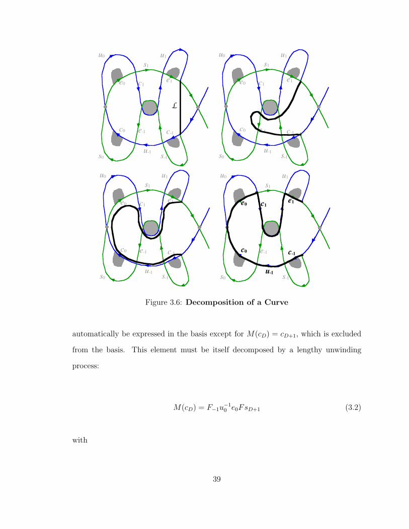
U−n, E−n) (Figure 3.6).

M acts on the decomposed path class l0 to advance the indices of each basis factor

in turn, e.g., M(e0s1) = e1s2 (recall l0 = e0s1). The forward iterates of l0 will

38

c1e1e0

e-1c0 c-1

u-1

u0 u1

s1

s0 s-1

L

c1e1e0

e-1c0 c-1

u-1

u0 u1

s1

s0 s-1

c1e1e0

e-1c0 c-1

u-1

u0 u1

s1

s0 s-1

c1e1e0

e-1c0 c-1

u-1

u0 u1

s1

s0 s-1

Figure 3.6: Decomposition of a Curve

automatically be expressed in the basis except for M(cD) = cD+1, which is excluded

from the basis. This element must be itself decomposed by a lengthy unwinding

process:

M(cD) = F−1u−10 e0FsD+1 (3.2)

with

39

F = c1e1c2e2...cDeD. (3.3)

One may verify that this decomposition is correct by looking at a picture.

3.0.5 Symbolic Representation of Escape

A path L of path class l intersects the escape zone E0 once for every occurrence of u0

or u−10 in its decomposition. This is clear from a graph of the tangle: the segment U0

bounds E0 on the outside; any path homotopic to U0 in the active region is forced to

cross through E0. Either u0 or u−10 may be present in the decomposition, depending

on the direction of L as it passes through E0: if L travels clockwise around hole H0

it will include u0; if it travels counterclockwise it will include the inverse, u−10 . Thus

many of the escape segments on a line of initial conditions L0 may be identified by

decomposing its path class l0 and mapping it forward, watching for the u0 segments.

Mitchell justifies this algorithm in an appendix in his paper; we simply list key results

here.

1. Iterate l0 N times; each un or u−1n factor (n > 0) in the expansion of lN corre-

sponds to a segment that escapes in N − n iterates.

2. The relative positions of the un-factors in the expansion of lN are the same as

the relative positions of their corresponding escape segments along L0.

40

3.0.6 Implications

With an algorithm to predict forced escape segments on nearly arbitrary lines of initial

conditions one may prove two rules about epistrophes in the discrete escape-time

plot, which Mitchell derives and names the Epistrophe Start Rule and the Epistrophe

Continuation Rule. His derivations are rigorous but both results may be understood

more simply.

Epistrophe Continuation Rule: Every segment (in the minimal set) that escapes at

N − 1 iterates has on its side a segment that escapes at N iterates. This is the

definition and origin of epistrophes in the escape-time plot. Consider a path class l

that includes the factor cD. When mapped forward, M(cD) = F−1u−10 e0FsD+1 —the

existence of a u0 term implies an escape segment. In fact, M(cD) is the only way

a u0 can arise in the basis of path classes, because all un, n < 0 are excluded from

the basis. Note as well that the definition F = c1e1c2e2...cDeD includes a cD term.

We reason: (1) the presence of an escape segment (a u0 factor) implies a preimage

factor cD; (2) each M(cD) includes two new cD factors which will include u0 factors

in one iteration; thus (3) the presence of an escape segment implies two more escape

segments in the subsequent iterate.

Epistrophe Start Rule: Every segment that escapes at N − ∆ iterates (∆ = D + 1)

spawns immediately on both of its sides a segment that escapes at N iterates. We

note that M(F ) = c−11 u−1

0 F and M(F−1) = F−1u0c1. Hence MD−1(F ) includes a

c−1D ; MD(F ) includes a u0 and, from M(cD) above, we see MD+1(cD) includes the

pair u0 and u−10 . These we identify as new epistrophes ∆ iterates after the original

escape segment.

41

The algorithm notably does not explain segments which are not forced by the holes.

A full epistrophic fractal may include strophes at arbitrary iterates, which may or

may not follow the Epistrophe Start Rule or Epistrophe Continuation Rule. It is

generally believed that to predict all the escape segments would require an infinity

of topological parameters; homotopic lobe dynamics today only considers the finite

decomposition of a line of initial conditions and the minimum delay time of the tangle,

so it is limited to description of the forced recursive structures.

3.0.7 Summary

Homotopic Lobe Dynamics identifies paths in the phase plane with path classes of like

topology. Path classes may be decomposed in a specially selected basis of path classes.

The action of M on these basis path classes is simply defined for all interesting classes

except cD, because cD+1 is excluded from the basis and must be decomposed into the

basis. Escape segments may be identified with occurrences of un and u−1n factors

in a path class decomposition. The algorithm for finding these segments becomes

the basis for the Epistrophe Continuation Rule and the Epistrophe Start Rule which

we see in the discrete escape-time plot. We can now apply this mathematics to the

surface of section for the fish cavity.

42

Chapter 4

Results And Analysis

We now turn to the analysis of our system. We have demonstrated that the time-

to-escape diagram has epistrophic fractal structure; we say the system obeys the

Epistrophe Continuation Rule and the Epistrophe Start Rule, and its forced escape

segments are predicted by Mitchell’s algorithm. Separately, we predict the form of

the pulse train that would be observed at the detector in the laboratory.

4.1 Confirming Epistrophic Structure

Recall that the minimum delay time D is determined by the first intersection H−D =

Cn ∩E−n in the surface of section, and this intersection maps forward and backward

to generate the full set of holes Hn. In our system the first intersection is C6 ∩ E−6,

therefore D = 2(6)− 1 = 11 (Figure 4.1).

The Epistrophe Start Rule predicts that escape segments in epistrophes spawn flank-

43

†

E0†

E1

†

E2

†

E3

†

E4

†

E5

†

C0

†

C1

†

C2

†

C3

†

C4

†

C5

†

C-1

†

C-2

†

C-3

†

C-4

†

C-5

†

E-1

†

E-2

†

E-3

†

E-4

†

E-50.8 0.82 0.84 0.86 0.88 0.9-0.1

-0.05

0

0.05

0.1

†

C-6 « E-6

Figure 4.1: Deriving D = 11

ing epistrophes ∆ = D + 1 iterates later. This holds in our system for all iterates we

simulate. Likewise, the Epistrophe Continuation Rule is responsible for the promi-

nent converging series of escape segments between the stable region and the regular

scattering regions of the line of initial conditions. Unsurprisingly, our plot has addi-

tional escape segments, some of them strophes, which are not part of these regular

sequences. One may note that some of them spawn their own epistrophes as though

following the rule; the current derivation of the Epistrophe Start Rule assumes that

parent escape segments belong to epistrophes already, but the topology of the homo-

clinic tangle may tend to impose similar conditions on strophes. Relevant structures

in our fractal are illustrated in (Figure 4.2).

44

-0.56 -0.54 -0.52 -0.5 -0.48 -0.46 -0.440

5

10

15

20

25

30

35

40

pl0

*

Figure 4.2: Epistrophic Fractal Time To Escape

We decompose our simple line of initial conditions into the product l0 = c0e0. It

was desirable to choose the simplest possible initial conditions because under many

iterations of M even a very simple curve may decompose into many terms. New sets

of escape segments appear every D+1 iterates, so for D = 11 the decomposition of the

initial conditions must map forward ten or twenty times before interesting features

will appear. Hence we chose to place L0 to the left of the stable zone (Figure 4.3).

By application of Mitchell’s algorithm one may find M(l0), M2(l0), etc1.

l0 = c0 (4.1)

1Following Mitchell, we omit terms en, n > 0 and all sn from the symbol sequences because theydo not result in escape segments or change the dynamics.

45

0 0.02 0.04 0.06 0.08 0.1 0.12 0.14 0.16 0.18 0.2

-0.5

-0.4

-0.3

-0.2

-0.1

0

0.1

0.2

0.3

0.4

0.5

l

L0

c0

e0

Figure 4.3: Decomposition of Initial Conditions

l1 = c1 (4.2)

l2 = c2 (4.3)

· · · (4.4)

l11 = c11 (4.5)

l12 = F−1u−10 F (first escape segment) (4.6)

l13 = F−1u−10 c1u

−11 c−1

1 u−10 F (4.7)

This decomposition finally includes a u0 at iterate 12, signifying one escape segment

on that iterate. The next, l13, has two u0s and a u−1 1, corresponding to the segment

on iterate 12 and two on iterate 13. One may verify by hand that

46

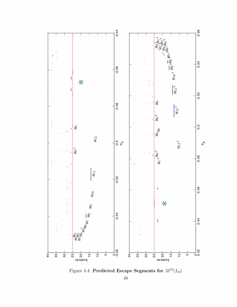
l25 = u0u1 · · ·u11u−10 u12u0u

−11 u−1

0 u−113 u0u1u

−10 u−1

12 u0u−111 u−1

10 · · ·u−10 (4.8)

This correctly predicts the order escape segments up to and including 25 iterates

(Figure 4.4). We focus on the two chaotic regions and omit the central stable region

of pl0.

47

-0.5

6-0

.54

-0.5

2-0

.5-0

.48

-0.4

6-0

.44

0510152025303540

p l0

u 1u 2

u 3u 4

u 5u 6

u 7u 8

u 9u 1

0u 1

1u 1

2

u 0u 0

-1u 0

0.42

0.44

0.46

0.48

0.5

0.52

0.54

0.56

0510152025303540

p l0

u 3-1

u 4-1 u 5

-1u 7

-1u 8

-1u 9

-1u 1

0-1u 1

1-1u 1

2-1u 1

3-1

u 6-1u 2

-1u 1

-1u 0

-1u 0

-1u 0

-1u 1

-1u 1

u 0u 0

*

*

Figure 4.4: Predicted Escape Segments for M25(L0)

48

4.2 The Pulse Train

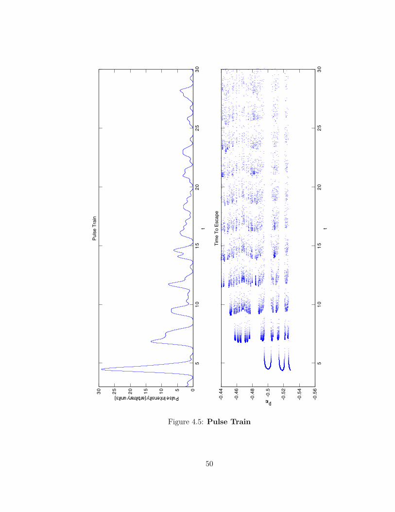
A histogram of time to escape over a set of trajectories gives a discretized representa-

tion of the pulse train seen at the detector. One burst of microwaves in a nonchaotic

system would escape in a fairly simple time distribution, still recognizable as a pulse

(though somewhat stretched out in time). Chaos—seen before in existence of discrete

escape segments—maps a burst of initial conditions to a lengthy pulse train at the

detector. Measurement of such a train should be possible in the laboratory and could

provide a sense of the dynamics in the system2.

Rather than use a histogram, we convolve the time to escape spectrum with a gaussian

to obtain a continuous pulse train function. One may note the correlation between

pulses and escape segments (Figure 4.5).

A uniformly distributed semicircular burst is not uniformly dense on the surface of

section. Here we picked initial conditions following a density function ρ = arccos pl

corresponding to a point flash of microwaves in all directions.

2Whether the pulse train may be transformed to yield an escape-time plot is an area of activeresearch.

49

510

1520

2530

-0.5

6

-0.5

4

-0.5

2

-0.5

-0.4

8

-0.4

6

-0.4

4

t

Tim

e To

Esc

ape

510

1520

2530

051015202530Pu

lse T

rain

t

Figure 4.5: Pulse Train

50

Chapter 5

Conclusions And Future Work

The fish-cavity system was conceived as a lab-friendly analogue to the ionization of

hydrogen in parallel electric and magnetic fields. We chose the shape of the reflecting

cavity to satisfy the conditions for a Saddle-Center Map as described in [3], notably

the presence of an unstable fixed point spawning a homoclinic tangle around a stable

zone. Under classical dynamics the time a particle takes to escape such a system is

highly sensitive to initial conditions; the plot of time to escape versus initial conditions

has epistrophic fractal structure. We identify, analyze and explain this structure in our

system, confirming that it is a suitable alternative to the hydrogen system. A single

burst of photons in the cavity will lead to a chaotic pulse train exiting the system.

We predict the shape of this pulse train for a particular line of initial conditions.

This simulation may be extended to predict steady-state interference patterns on a

planar detector. Interference effects cannot be modeled by simply assigning a phase to

trajectories. A correct model has to include Maslov indices, which requires analysis of

the optical properties of the fish cavity. This extension would be a valuable addition

51

to the simulator.

Finally, this system remains to be tested. Being two-dimensional it is well-suited to

tabletop microwave experiments and in fact bears resemblance to experiments being

done now by Prof. Srinivas Sridhar of Northeastern University. Such an experiment

would provide a valuable test of Homotopic Lobe Dynamics. We look forward to

seeing our system tested fully in the laboratory.

52

Appendix: Implementation Notes

5.1 Trajectories

We represent trajectories parametrically by their current position −→x and velocity

−→v (normalized to the speed c = 1.0 in simulation units). The simulator calculates

the time ∆t for a trajectory to intersect the wall of the cavity and advances the

trajectories as

x1 = x0 + vx∆t (5.1)

v1 = v0 + vy∆t (5.2)

The cavity is represented by the “fish function”

y = f(x) = ±√

x(w

2+ A(x− L)2

)(5.3)

We substitute the parametric equations 5.1 into the fish function 5.3 to find the

53

intersection of the trajectory with the wall. The numerics are simplified by squaring

the resulting equation, thereby obtaining the “intersection polynomial”

P (t) = (y − f)2 = 0 (5.4)

which conveniently eliminates the need to distinguish between intersections on the

y > 0 and y < 0 sections of the cavity. Finding roots of polynomials numerically

is fast and accurate; Matlab has functions to handle this for us. This fifth-degree

polynomial in t has, in general, real and complex roots, which we classify as follows:

• Positive real roots: intersections in the future, ∆t > 0

• Negative real roots: intersections in the past, ∆t < 0

• Vanishing real roots: the trajectory’s current position on the wall

• Complex roots: no physical intersection

The smallest positive real root ∆t = tmin corresponds to the first intersection of

the trajectory with the fish curve in the future, by which we may calculate the new

position. Sometimes the current position on the wall, the root t = 0, appears as an

intersection in the future (albeit with very small 0 < t � 1). We omit these roots

by requiring tmin to surpass a threshold value tsmall = 10−12. In practice this allows

extremely tangential trajectories (whispering gallery modes) to pass through the wall,

but such trajectories are outside our region of interest and we do not create them.

Reflection conserves speed, so we reverse the trajectory’s velocity normal to the curve,

v⊥:

54

−→v next = −→v ‖ −−→v ⊥ = 2(−→v · f‖)v −−→v (5.5)

where−→f ‖, the tangent vector to the fish curve, may be calculated by either of two

formulations:

−→f ‖ =

(1,

dy

dx

)=

(1,

df

dx

)(5.6)

−→f ‖ =

(dx

dy, 1

)=

(2y

(d

dxf(x)2

)−1

, 1

). (5.7)

Analytically, the methods lead to the same f‖, but the numerical error is different.

In the regime x � 1,

∆dy

dx∝ x−1/2 (5.8)

∆dx

dy∝ 1. (5.9)

At points where the curve flattens so dfdx' 0, there is a singularity in dx

dy. We chose

the most accurate method for different sections of the curve by considering a plot of

1 − dydx

dxdy

(Figure 5.1) and estimating the point at which error was minimized. For

small x, most of the error comes from dydx

, but for larger x the error is due to dxdy

. In

practice we use xcutoff = xstable/3 as it remains a good approximation for various L

(bottleneck positions).

55

0 0.05 0.1 0.15 0.2 0.25-5

-4

-3

-2

-1

0

1

2

3

4

5 x 10-14Comparison of Slope-Finding Methods, culled to 5e-14, x < stablepoint

X

Figure 5.1: Choosing Cutoff Point

5.2 Surface Of Section

Arc-length momentum pl in the surface of section is identical to v‖ as calculated above,

and we use the same precautions to maximize accuracy. The arc-length coordinate l

is the path length along the curve wall, found by either of two integrals:

l(x) =

∫ xorbit

x=0

√1 +

(dy

dx

)2

dx (5.10)

l(y) =

∫ yorbit

y=0

√1 +

(dx

dy

)2

dy. (5.11)

Neither of these can be evaluated analytically, so we integrate them numerically using

Matlab’s ODE solvers. For x < xcutoff , we use l(y). Unfortunately, simply integrating

l(x) as in equation 5.10 still relies on dydx

near the origin and is prone to error. Thus

we split the calculation into two parts:

56

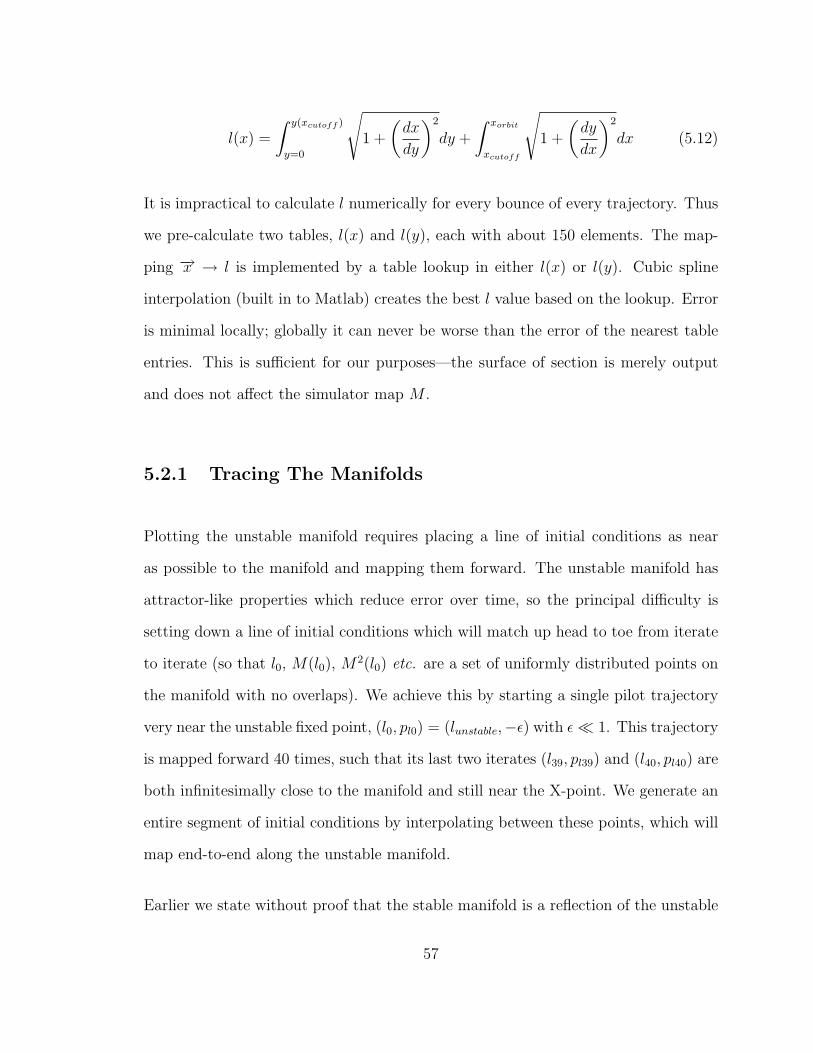
l(x) =

∫ y(xcutoff )

y=0

√1 +

(dx

dy

)2

dy +

∫ xorbit

xcutoff

√1 +

(dy

dx

)2

dx (5.12)

It is impractical to calculate l numerically for every bounce of every trajectory. Thus

we pre-calculate two tables, l(x) and l(y), each with about 150 elements. The map-

ping −→x → l is implemented by a table lookup in either l(x) or l(y). Cubic spline

interpolation (built in to Matlab) creates the best l value based on the lookup. Error

is minimal locally; globally it can never be worse than the error of the nearest table

entries. This is sufficient for our purposes—the surface of section is merely output

and does not affect the simulator map M .

5.2.1 Tracing The Manifolds

Plotting the unstable manifold requires placing a line of initial conditions as near

as possible to the manifold and mapping them forward. The unstable manifold has

attractor-like properties which reduce error over time, so the principal difficulty is

setting down a line of initial conditions which will match up head to toe from iterate

to iterate (so that l0, M(l0), M2(l0) etc. are a set of uniformly distributed points on

the manifold with no overlaps). We achieve this by starting a single pilot trajectory

very near the unstable fixed point, (l0, pl0) = (lunstable,−ε) with ε � 1. This trajectory

is mapped forward 40 times, such that its last two iterates (l39, pl39) and (l40, pl40) are

both infinitesimally close to the manifold and still near the X-point. We generate an

entire segment of initial conditions by interpolating between these points, which will

map end-to-end along the unstable manifold.

Earlier we state without proof that the stable manifold is a reflection of the unstable

57

manifold. The stable manifold is the set of all trajectories that map forward asymp-

totically to the X-point. In reverse time, the stable manifold looks like the unstable

manifold—the set of trajectories diverging from the X-point—except that momentum

vectors still point “forward.” We can therefore plot the stable manifold by reversing

momenta of trajectories diverging from the X-point. On the surface of section, this

is the reflection (pl → −pl) of the unstable manifold.

5.2.2 Intersections With E0

For a trajectory in the complex, we define escape as entering the escape zone E0. We

pre-plotted the unstable manifold (hence the stable manifold) to very high resolution

and saved the sections bounding E0. For efficiency we detecting escapes with a two-

step process:

1. Bounding Box Check: does the trajectory fall into the rectangular bounding box

around E0? This step rapidly removes most trajectories from consideration.

2. Manifold Check: does the trajectory pass to the right of the unstable manifold

and to the left of the stable manifold? This step uses cubic spline interpolation

for maximum accuracy and is considerably slower than the bounding box check.

In a typical simulation of 10,000 trajectories, there are usually only one or two inci-

dents when the simulator catches the same trajectory in the escape zone twice. The

occasional error is most likely due to the resolution on the manifold segments and

does not affect our analysis of the time to escape.

58

59

Bibliography

[1] Melissa Commisso, REU project report, College of William and Mary, 2003.

(unpublished)

[2] Joel Handley, REU project report, College of William and Mary, 2001.

(unpublished)

[3] K.A. Mitchell, J.P. Handley, J.B. Delos, S.K. Knudson, Chaos 13, 880 (2003).

[4] K.A. Mitchell, J.P. Handley, J.B. Delos, S.K. Knudson, Chaos 13, 892 (2003).

[5] K.A. Mitchell, J.P. Handley, B. Tighe, A.A. Flower, J.B. Delos, Phys. Rev.

Lett. 92, 073001 (2004)

[6] A. Tiyapan, Charles Jaffe, J. Chem. Phys. 99, 2765 (1993).

60