ARTICLE IN PRESS

0921-4526/$ - se

doi:10.1016/j.ph

�CorrespondiE-mail addre

Physica B 396 (2007) 57–61

www.elsevier.com/locate/physb

Chaos suppression by feedback control in nuclear magnetic resonance

Ling Peng, Shuhui Cai, Zhong Chen�

Department of Physics, State Key Laboratory of Physical Chemistry of Solid Surface, Xiamen University, Xiamen, Fujian 361005, PR China

Received 14 January 2007; received in revised form 26 February 2007; accepted 5 March 2007

Abstract

The strength of static magnetic field and the sensitivity of probe increase with the technique development of modern nuclear magnetic

resonance (NMR) spectrometer. Radiation damping effect thus can no longer be neglected in solution NMR experiments with abundant

spins. The cooperative effects of radiation damping and distant dipolar field (DDF) generate spin turbulence, which makes the evolution

of magnetization unpredictable by traditional NMR theory and causes the uncertainty of acquired signals. The chaos phenomena can be

described by introducing a radiation damping term into the Bloch equations. In this paper, we used two kinds of feedback control

method to suppress the chaotic process. Numerical simulation indicates their feasibility and efficiency.

r 2007 Published by Elsevier B.V.

PACS: 76.60.�k; 76.80.+y; 75.40.Gb; 39.30.+w

Keywords: Feedback control; Nuclear magnetic resonance; Chaos; Numerical simulation; Suppression

1. Introduction

In solution nuclear magnetic resonance (NMR), strongstatic magnetic field and high sensitive probe help offsetintrinsic limitations in signal sensitivity and resolution. Atthe same time, increasing magnetic field strength and probesensitivity also intensify concentrated solvent effects arisingfrom large bulk sample magnetization [1]. As we know, inmodern solution NMR experiments with abundant high-gyromagnetic ratio (g) spins, radiation damping anddistant dipolar field (DDF) are dominant bulk solventeffects. Radiation damping is a macroscopic reaction fieldthat acts back on spins through the induced current inreceiver coil, while DDF results from long range dipolarinteractions existing between distant spins [1,2]. Thecooperation of radiation damping and DDF generatesspin turbulence [3]. As a result, the received signals becomechaotic. In addition, in many polarization experimentsNMR dynamics is deeply affected by strong dipolarcouplings [4–6], making spectra clustering and instabilities[5,7]. Dynamical instabilities are also related to fieldgradients in liquid NMR experiments with large nuclear

e front matter r 2007 Published by Elsevier B.V.

ysb.2007.03.032

ng author. Tel.: +86592 2181712; fax: +86 592 2189426.

ss: chenz@xmu.edu.cn (Z. Chen).

magnetization [8]. Ardelean et al. ever reported multiplespin echoes phenomena arising after ‘‘nonlinear’’ evolutionof modulated demagnetizing field, for example, with theaid of a sequence of two 901 radio-frequency (RF) pulses inthe presence of pulsed or steady field gradients [9–11], andthis system likely turns chaotic. Ugulava et al. [12] showedthat conditions of chaos emergence were defined by twoparameters: amplitude of RF field and detuning. Therefore,these two experimental parameters are of importance forchaos control. In some instances, chaotic phenomena canbe described when a radiation damping term is introducedinto the Bloch equations [3,13]. Such nonlinear Blochequations can be studied not only by using perturbationtheory [12], but also by numerical simulation. In this paper,numerical simulation was carried out. Feedback controlmethod was employed to suppress chaotic process withoutchanging amplitude of RF field and detuning, which maybe realized in NMR spectrometer.

2. Description of NMR by nonlinear Bloch equations

Generally, spin evolution can be described by the classicBloch equations. However, a radiation damping term mustbe introduced when strong radiation damping effect exists.

ARTICLE IN PRESS

t = 6s t = 10s

t = 15s t = 20s

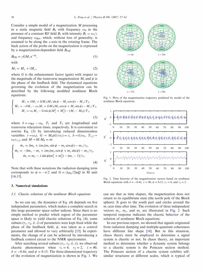
Fig. 1. Plots of the magnetization trajectory predicted by model of the

nonlinear Bloch equations.

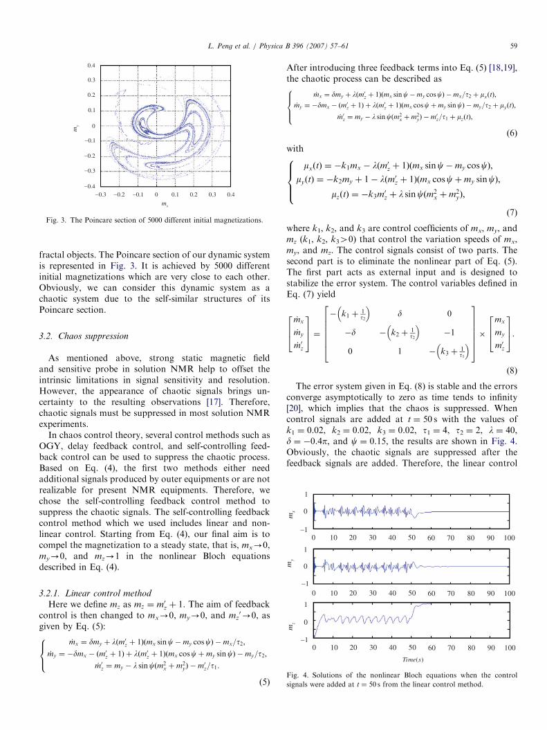
Fig. 2. Time histories of the magnetization vectors based on nonlinear

Bloch equations with d ¼ �0.4p, l ¼ 40, c ¼ 0.15, t1 ¼ 4, and t2 ¼ 2.

L. Peng et al. / Physica B 396 (2007) 57–6158

Consider a simple model of a magnetization M precessingin a static magnetic field B0 with frequency o0 in thepresence of a constant RF field B1 with intensity B1 ¼ o1/gand frequency oRF, which, without loss of generality, isassumed to be along the x-axis in the rotating frame. Theback action of the probe on the magnetization is expressedby a magnetization-dependent field BFB:

BFB ¼ gGMt e�ic, (1)

with

M t ¼Mx þ iMy, (2)

where G is the enhancement factor (gain) with respect tothe magnitude of the transverse magnetization Mt and c isthe phase of the feedback field. The dynamical equationsgoverning the evolution of the magnetization can bedescribed by the following modified nonlinear Blochequations:

_Mx ¼ dMy þ GMzðMx sinc�My coscÞ �Mx=T2;_My ¼ �dMx � o1Mz þ GMzðMx coscþMy sincÞ �My=T2;

_Mz ¼ o1My � G sincðM2x þM2

yÞ � ðMz �M0Þ=T1;

8>><>>:

(3)

where d ¼ oRF � o0, T1 and T2 are longitudinal andtransverse relaxation times, respectively. It is convenient torewrite Eq. (3) by introducing reduced dimensionlessvariables: t-o1t, G!M0ðG=o1Þ ¼ l, d-d/o1, T1,2-o1t1,2, and M-M/M0 ¼ m:

_mx ¼ dmy þ lmzðmx sinc�my coscÞ �mx=t2;

_my ¼ �dmx �mz þ lmzðmx coscþmy sincÞ �my=t2;

_mz ¼ my � l sincðm2x þm2

yÞ � ðmz � 1Þ=t1:

8><>:

(4)

Note that with these notations the radiation damping termcorresponds to c ¼ �p/2 and G ¼ gðm0=2ÞZQ in SI unit[14,15].

3. Numerical simulations

3.1. Chaotic solutions of the nonlinear Bloch equations

As we can see, the dynamics of Eq. (4) depends on fiveindependent parameters, which makes a complete search inthis large parameter space rather tedious. Since there is nosimple method to predict which region of the parameterspace is likely to yield chaotic solutions of Eq. (4), somesubsets (t1, t2, d, l) of parameters were kept fixed while thephase of the feedback field, c, was taken as a controlparameter and allowed to vary arbitrarily [15]. In experi-ments, the change of c can be achieved by introducing afeedback control circuit to the NMR spectrometer.

After searching several subsets (t1, t2, d, l), we observedchaotic phenomenon when t1 ¼ 4, t2 ¼ 2, l ¼ 40,d ¼ �0.4p, and c ¼ 0.15. The three-dimensional trajectoryof the evolution of magnetization is shown in Fig. 1. We

can see that as time elapses, the magnetization does notreturn to its equilibrium state (the north pole of the Blochsphere). It goes to the south part and circles around themz-axis time after time. The evolution of three independentvectors mx, my, and mz are illustrated in Fig. 2. Suchtemporal response indicates the chaotic behavior of thesolution of nonlinear Bloch equations.In our previous report, we showed that signals originated

from radiation damping and multiple-quantum coherenceshave different line shape [16]. But in this situation,chaos theory must be employed to determine a signalsystem is chaotic or not. In chaos theory, an importantmethod to determine whether a dynamic system belongsto a chaotic system is the Poincare section method.The Poincare section of a chaotic system exhibits self-similar structures at different scales, which is typical of

ARTICLE IN PRESS

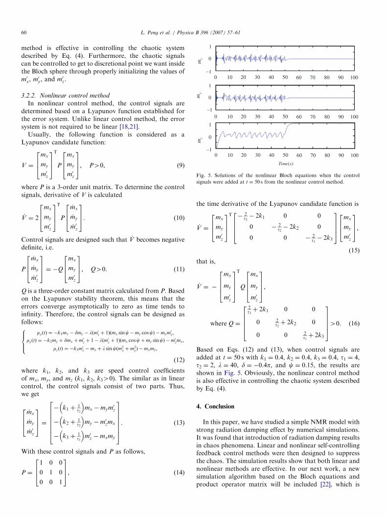
Fig. 3. The Poincare section of 5000 different initial magnetizations.

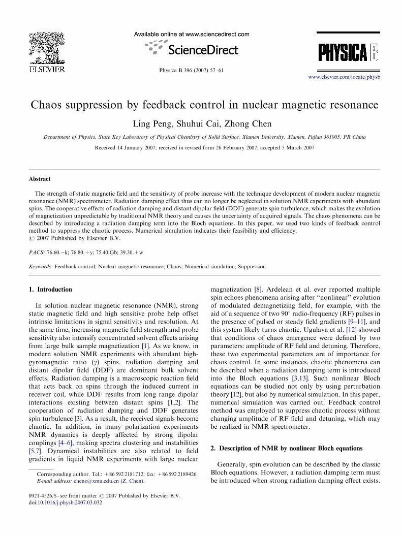
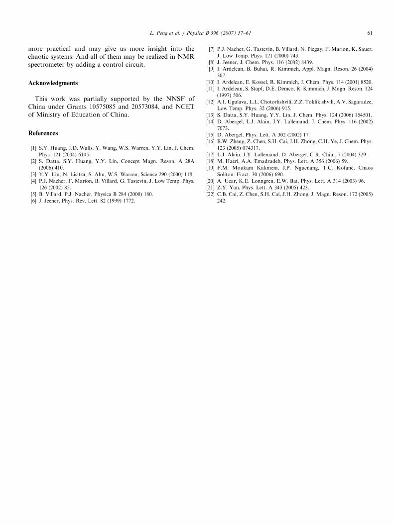
Fig. 4. Solutions of the nonlinear Bloch equations when the control

signals were added at t ¼ 50 s from the linear control method.

L. Peng et al. / Physica B 396 (2007) 57–61 59

fractal objects. The Poincare section of our dynamic systemis represented in Fig. 3. It is achieved by 5000 differentinitial magnetizations which are very close to each other.Obviously, we can consider this dynamic system as achaotic system due to the self-similar structures of itsPoincare section.

3.2. Chaos suppression

As mentioned above, strong static magnetic fieldand sensitive probe in solution NMR help to offset theintrinsic limitations in signal sensitivity and resolution.However, the appearance of chaotic signals brings un-certainty to the resulting observations [17]. Therefore,chaotic signals must be suppressed in most solution NMRexperiments.

In chaos control theory, several control methods such asOGY, delay feedback control, and self-controlling feed-back control can be used to suppress the chaotic process.Based on Eq. (4), the first two methods either needadditional signals produced by outer equipments or are notrealizable for present NMR equipments. Therefore, wechose the self-controlling feedback control method tosuppress the chaotic signals. The self-controlling feedbackcontrol method which we used includes linear and non-linear control. Starting from Eq. (4), our final aim is tocompel the magnetization to a steady state, that is, mx-0,my-0, and mz-1 in the nonlinear Bloch equationsdescribed in Eq. (4).

3.2.1. Linear control method

Here we define mz as mz ¼ m0z þ 1. The aim of feedbackcontrol is then changed to mx-0, my-0, and mz

0-0, asgiven by Eq. (5):

_mx ¼ dmy þ lðm0z þ 1Þðmx sinc�my coscÞ �mx=t2;

_my ¼ �dmx � ðm0z þ 1Þ þ lðm0z þ 1Þðmx coscþmy sincÞ �my=t2;

_m0z ¼ my � l sincðm2x þm2

yÞ �m0z=t1:

8><>:

(5)

After introducing three feedback terms into Eq. (5) [18,19],the chaotic process can be described as

_mx ¼ dmy þ lðm0z þ 1Þðmx sinc�my coscÞ �mx=t2 þ mxðtÞ;

_my ¼ �dmx � ðm0z þ 1Þ þ lðm0z þ 1Þðmx coscþmy sincÞ �my=t2 þ myðtÞ;

_m0z ¼ my � l sincðm2x þm2

yÞ �m0z=t1 þ mzðtÞ;

8>><>>:

(6)

with

mxðtÞ ¼ �k1mx � lðm0z þ 1Þðmx sinc�my coscÞ;

myðtÞ ¼ �k2my þ 1� lðm0z þ 1Þðmx coscþmy sincÞ;

mzðtÞ ¼ �k3m0z þ l sincðm2

x þm2yÞ;

8>><>>:

(7)

where k1, k2, and k3 are control coefficients of mx, my, andmz (k1, k2, k340) that control the variation speeds of mx,my, and mz. The control signals consist of two parts. Thesecond part is to eliminate the nonlinear part of Eq. (5).The first part acts as external input and is designed tostabilize the error system. The control variables defined inEq. (7) yield

_mx

_my

_m0z

264

375 ¼

� k1 þ1t2

� �d 0

�d � k2 þ1t2

� ��1

0 1 � k3 þ1t1

� �

2666664

3777775�

mx

my

m0z

264

375.

(8)

The error system given in Eq. (8) is stable and the errorsconverge asymptotically to zero as time tends to infinity[20], which implies that the chaos is suppressed. Whencontrol signals are added at t ¼ 50 s with the values ofk1 ¼ 0.02, k2 ¼ 0.02, k3 ¼ 0.02, t1 ¼ 4, t2 ¼ 2, l ¼ 40,d ¼ �0.4p, and c ¼ 0.15, the results are shown in Fig. 4.Obviously, the chaotic signals are suppressed after thefeedback signals are added. Therefore, the linear control

ARTICLE IN PRESS

Fig. 5. Solutions of the nonlinear Bloch equations when the control

signals were added at t ¼ 50 s from the nonlinear control method.

L. Peng et al. / Physica B 396 (2007) 57–6160

method is effective in controlling the chaotic systemdescribed by Eq. (4). Furthermore, the chaotic signalscan be controlled to get to discretional point we want insidethe Bloch sphere through properly initializing the values ofm0x, m0y, and m0z.

3.2.2. Nonlinear control method

In nonlinear control method, the control signals aredetermined based on a Lyapunov function established forthe error system. Unlike linear control method, the errorsystem is not required to be linear [18,21].

Usually, the following function is considered as aLyapunov candidate function:

V ¼

mx

my

m0z

264

375T

P

mx

my

m0z

264

375; P40, (9)

where P is a 3-order unit matrix. To determine the controlsignals, derivative of V is calculated

_V ¼ 2

mx

my

m0z

264

375T

P

_mx

_my

_m0z

264

375. (10)

Control signals are designed such that _V becomes negativedefinite, i.e.

P

_mx

_my

_m0z

264

375 ¼ �Q

mx

my

m0z

264

375; Q40. (11)

Q is a three-order constant matrix calculated from P. Basedon the Lyapunov stability theorem, this means that theerrors converge asymptotically to zero as time tends toinfinity. Therefore, the control signals can be designed asfollows:

mxðtÞ ¼ �k1mx � dmy � lðm0z þ 1Þðmx sinc�my coscÞ �mym0z;

myðtÞ ¼ �k2my þ dmx þm0z þ 1� lðm0z þ 1Þðmx coscþmy sincÞ �m0zmx;

mzðtÞ ¼ �k3m0z �my þ l sincðm2x þm2

yÞ �mxmy;

8>><>>:

(12)

where k1, k2, and k3 are speed control coefficientsof mx, my, and mz (k1, k2, k340). The similar as in linearcontrol, the control signals consist of two parts. Thus,we get

_mx

_my

_m0z

264

375 ¼

� k1 þ1t2

� �mx �mym0z

� k2 þ1t2

� �my �m0zmx

� k3 þ1t1

� �m0z �mxmy

2666664

3777775. (13)

With these control signals and P as follows,

P ¼

1 0 0

0 1 0

0 0 1

264

375, (14)

the time derivative of the Lyapunov candidate function is

_V ¼

mx

my

m0z

264

375T � 2

t2� 2k1 0 0

0 � 2t2� 2k2 0

0 0 � 2t1� 2k3

2664

3775

mx

my

m0z

264

375,

(15)

that is,

_V ¼ �

mx

my

m0z

2664

3775

T

Q

mx

my

m0z

2664

3775,

where Q ¼

2t2þ 2k1 0 0

0 2t2þ 2k2 0

0 0 2t1þ 2k3

26664

3777540. ð16Þ

Based on Eqs. (12) and (13), when control signals areadded at t ¼ 50 s with k1 ¼ 0.4, k2 ¼ 0.4, k3 ¼ 0.4, t1 ¼ 4,t2 ¼ 2, l ¼ 40, d ¼ �0.4p, and c ¼ 0.15, the results areshown in Fig. 5. Obviously, the nonlinear control methodis also effective in controlling the chaotic system describedby Eq. (4).

4. Conclusion

In this paper, we have studied a simple NMR model withstrong radiation damping effect by numerical simulations.It was found that introduction of radiation damping resultsin chaos phenomena. Linear and nonlinear self-controllingfeedback control methods were then designed to suppressthe chaos. The simulation results show that both linear andnonlinear methods are effective. In our next work, a newsimulation algorithm based on the Bloch equations andproduct operator matrix will be included [22], which is

ARTICLE IN PRESSL. Peng et al. / Physica B 396 (2007) 57–61 61

more practical and may give us more insight into thechaotic systems. And all of them may be realized in NMRspectrometer by adding a control circuit.

Acknowledgments

This work was partially supported by the NNSF ofChina under Grants 10575085 and 20573084, and NCETof Ministry of Education of China.

References

[1] S.Y. Huang, J.D. Walls, Y. Wang, W.S. Warren, Y.Y. Lin, J. Chem.

Phys. 121 (2004) 6105.

[2] S. Datta, S.Y. Huang, Y.Y. Lin, Concept Magn. Reson. A 28A

(2006) 410.

[3] Y.Y. Lin, N. Lisitza, S. Ahn, W.S. Warren, Science 290 (2000) 118.

[4] P.J. Nacher, F. Marion, B. Villard, G. Tastevin, J. Low Temp. Phys.

126 (2002) 85.

[5] B. Villard, P.J. Nacher, Physica B 284 (2000) 180.

[6] J. Jeener, Phys. Rev. Lett. 82 (1999) 1772.

[7] P.J. Nacher, G. Tastevin, B. Villard, N. Piegay, F. Marion, K. Sauer,

J. Low Temp. Phys. 121 (2000) 743.

[8] J. Jeener, J. Chem. Phys. 116 (2002) 8439.

[9] I. Ardelean, B. Buhai, R. Kimmich, Appl. Magn. Reson. 26 (2004)

307.

[10] I. Ardelean, E. Kossel, R. Kimmich, J. Chem. Phys. 114 (2001) 8520.

[11] I. Ardelean, S. Stapf, D.E. Demco, R. Kimmich, J. Magn. Reson. 124

(1997) 506.

[12] A.I. Ugulava, L.L. Chotorlishvili, Z.Z. Toklikishvili, A.V. Sagaradze,

Low Temp. Phys. 32 (2006) 915.

[13] S. Datta, S.Y. Huang, Y.Y. Lin, J. Chem. Phys. 124 (2006) 154501.

[14] D. Abergel, L.J. Alain, J.Y. Lallemand, J. Chem. Phys. 116 (2002)

7073.

[15] D. Abergel, Phys. Lett. A 302 (2002) 17.

[16] B.W. Zheng, Z. Chen, S.H. Cai, J.H. Zhong, C.H. Ye, J. Chem. Phys.

123 (2005) 074317.

[17] L.J. Alain, J.Y. Lallemand, D. Abergel, C.R. Chim. 7 (2004) 329.

[18] M. Haeri, A.A. Emadzadeh, Phys. Lett. A 356 (2006) 59.

[19] F.M. Moukam Kakmeni, J.P. Nguenang, T.C. Kofane, Chaos

Soliton. Fract. 30 (2006) 690.

[20] A. Ucar, K.E. Lonngren, E.W. Bai, Phys. Lett. A 314 (2003) 96.

[21] Z.Y. Yan, Phys. Lett. A 343 (2005) 423.

[22] C.B. Cai, Z. Chen, S.H. Cai, J.H. Zhong, J. Magn. Reson. 172 (2005)

242.