Bulletin de la Classe des Sciences de l’Academie Royale de Belgique, 6e serie, tome XI (2000) 9-48

CHAOS, FRACTALS AND THERMODYNAMICS

Pierre GASPARDCenter for Nonlinear Phenomena and Complex Systems,

Universite Libre de Bruxelles,Campus Plaine C. P. 231, Blvd du Triomphe,

B-1050 Brussels, Belgium

I. TEMPORAL EVOLUTION OF NATURAL SYSTEMS

A. Historical introduction

Since Newton, the temporal evolution of natural systems has been described by mathematical laws expressed interms of differential equations. The equations uniquely determine the system state at time t+ dt as a function of itsprevious state at time t. The state of the system is defined by a set of coordinates X taking their values in the so-calledphase space [1]. These coordinates are for instance the positions and velocities of the particles of a mechanical system.A typical differential equation is of the form

dXdt

= F(X) , (1)

with dX = X(t+ dt)−X(t) and where F(X) is the function which determines the change of state X per unit time.The Newtonian scheme has been fabulously successful not only in celestial mechanics, but also in the mechanics ofcontinuous media, in electromagnetism and, throughout the XXth century, in Einstein’s relativity theories and inquantum mechanics.

Beside the systems successfully described by the Newtonian scheme, numerous natural phenomena of randomcharacter have been quantitatively studied by this other mathematical scheme which is statistics, developed duringthe XIXth century notably by Quetelet. At the end of the XIXth century, the founding fathers of statistical mechanics– Maxwell, Boltzmann, and Gibbs – performed the integration of statistics with Newtonian mechanics. The adventof statistical mechanics allowed the study of large systems of particles and the derivation of the macroscopic laws ofevolution – such as the Navier-Stokes equations of fluid mechanics – on the basis of the microscopic motion of theparticles composing matter. In particular, the pressure or the internal energy, as well as the viscosity or the thermalconductivity could be derived from the properties of the microscopic particles such as their size, their mass and theirinteraction force.

In retrospect, the success of statistical mechanics is based on the fact that the macroscopic behavior results fromthe local conservation of the mass, the energy, and the three linear momenta, which form five constants of motion. Ifthe underlying system was completely integrable, many further constants of motion would exist resulting in specialtransport phenomena very different from the normal transport phenomena predicted by Boltzmann nonequilibriumstatistical mechanics. The origin of the non-existence of further constants of motion was discovered in celestialmechanics by Henri Poincare who recognized the importance of the role played by unstable periodic orbits in hisstudy of the three-body problem [2]. Poincare discovered that each unstable periodic orbit is a kind of crossing wheretrajectories arrive and depart after a time of passage much varying according to the minimal distance reached by thetrajectory with respect to the unstable periodic orbit (see Fig. 1). The trajectories do not remain confined near suchunstable periodic orbits and they can thus wander from one unstable periodic orbit to another. Let us mention thatthis process is used to plan space missions such as the GENESIS mission for the study of the solar wind. This missionwill start in January 2001 for three years. The space probe will be sent onto an unstable halo periodic orbit betweenEarth and Sun. The instability of the halo periodic orbit allows the arrival and the departure of the space probe witha minimum of fuel [3].

In a system with unstable periodic orbits, a very complex recurrent motion takes place if a circuit allows the trajec-tories to come back near the unstable periodic orbit. Such loop circuits have been called homoclinic orbits by Poincareand they are at the origin of aperiodic recurrent motions called chaotic motions as proved thereafter by Birkhoff [4].More recently, Moser proved that homoclinic orbits break the further constants of motion in the mechanical system[5]. This general result shows the essential role played by the dynamical instability for the generation of statistical

2

behaviors in a mechanical system such as the three-body system. This result extends a fortiori to the larger systemsof particles of statistical mechanics and it explains why all the further constants of motion beside the five fundamentalones are broken, justifying this behavior of Boltzmann’s nonequilibrium statistical mechanics.

C

P

H

W u

W s

π

FIG. 1: Phase portrait of a mechanical system with an unstable periodic orbit P , its stable Ws and unstable Wu manifolds, ahomoclinic orbit H and the resulting homoclinic tangle C. The stable (resp. unstable) manifolds are the continuous familiesof trajectories which converge to (resp. diverge from) the unstable periodic orbit. π is the Poincare section across all thetrajectories.

One could have believed that unstable dynamical behavior is rare in natural systems. However, since the sixtiesand the advent of numerical computers, many works by Lorenz [6], Shil’nikov [7], Smale [8], Henon [9] and others haveshown that the dissipative and Hamiltonian dynamical systems typically present unstable periodic orbits, homoclinicorbits and, as a consequence, chaotic behavior. Chaos has thus become a major preoccupation in many scientificdomains from mathematics to physics, astrophysics, geophysics, chemistry, biology, medicine, and also social andeconomic sciences.

B. Sensitivity to initial conditions and random behavior

A great effort has been devoted to the characterization of dynamical chaos [10]. Several quantities have beenproposed and, especially, the Lyapunov exponents and the Kolmogorov-Sinai entropy per unit time.

The concept of Lyapunov exponent goes back to a work in 1892 on the stability and instability of motion byLyapunov [11]. This concept was introduced to characterize the linear stability or instability of a trajectory. ALyapunov exponent is the growth rate of an infinitesimal perturbation on a reference trajectory. There are as manypossible different Lyapunov exponents as linearly independent infinitesimal perturbations on a trajectory. The numberof these exponents is thus equal to the phase-space dimension. Of course, since most systems are not explosive, thereexist at least as many negative as positive Lyapunov exponents. In Hamiltonian systems, the symplectic character ofthe time evolution implies that there are precisely as many non-positive as non-negative Lyapunov exponents. Theset of Lyapunov exponents form the so-called Lyapunov spectrum. If the largest Lyapunov exponent is positive λ+

1 ,an infinitesimal perturbation on the trajectory will have an exponential growth according to

‖δX(t)‖ ' ‖δX(0)‖ exp(λ+1 t) , (2)

so that an error on the initial conditions X(0) will amplify and the perturbed trajectory will separate from thereference trajectory. This property of unstable systems is referred to as the sensitivity to the initial conditions and itlimits the prediction on the future time evolution of the system. This sensitivity to initial condition is well-known inmeteorology.

If we wish to make a prediction with the final precision εfinal starting from initial conditions known with the precisionεinitial, we observe from Eq. (2) that a certain time cannot be exceeded:

3

t < tmax =1λ+

1

lnεfinal

εinitial, (3)

which constitutes a temporal horizon on the prediction. This horizon can be delayed but to the price of an exponentiallyimproved knowledge on the initial conditions, which means that the required number of decimals on the initialconditions should increase linearly with the maximum prediction time tmax. In practice, the horizon thus remainsof the order of the inverse of the maximum Lyapunov exponent: the larger the Lyapunov exponent, the closer thehorizon.

Beyond this horizon, several trajectories from nearby initial conditions separated by the initial precision εinitial willdisperse in the phase space. If the motion remains nevertheless bounded in the vicinity of a homoclinic loop circuit,the trajectories undergo aperiodic recurrences. The resulting temporal chaos is characterized by a concept which is apriori different from the one of Lyapunov exponent. This new concept is the so-called Kolmogorov-Sinai (KS) entropyper unit time [10, 12], which has its origin in the concept of entropy per unit time introduced by Claude Shannon inhis information theory. Shannon introduced his entropy per unit time in analogy with Boltzmann’s entropy per unitvolume which characterizes a spatial disorder. In contrast, Shannon’s entropy per unit time characterizes a temporaldisorder, for instance, in the time evolution of a chaotic system.

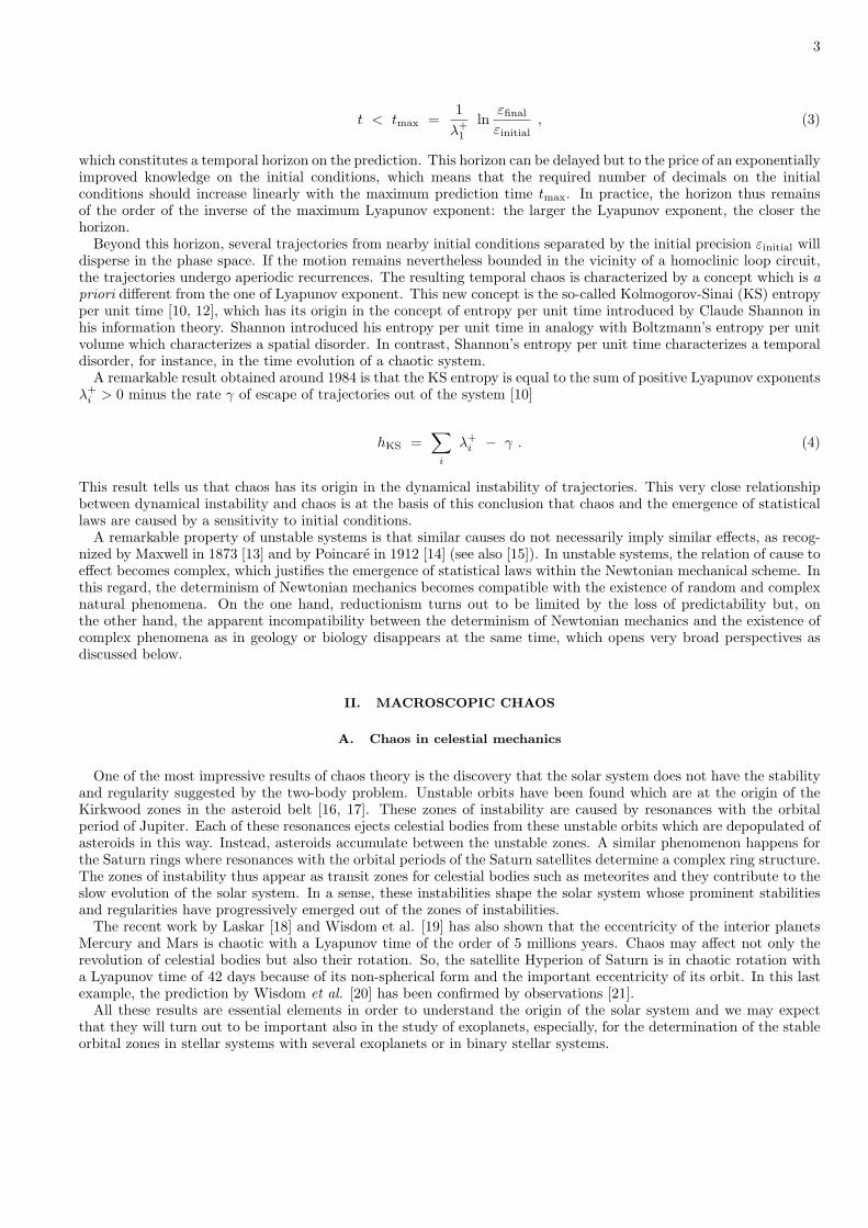
A remarkable result obtained around 1984 is that the KS entropy is equal to the sum of positive Lyapunov exponentsλ+i > 0 minus the rate γ of escape of trajectories out of the system [10]

hKS =∑i

λ+i − γ . (4)

This result tells us that chaos has its origin in the dynamical instability of trajectories. This very close relationshipbetween dynamical instability and chaos is at the basis of this conclusion that chaos and the emergence of statisticallaws are caused by a sensitivity to initial conditions.

A remarkable property of unstable systems is that similar causes do not necessarily imply similar effects, as recog-nized by Maxwell in 1873 [13] and by Poincare in 1912 [14] (see also [15]). In unstable systems, the relation of cause toeffect becomes complex, which justifies the emergence of statistical laws within the Newtonian mechanical scheme. Inthis regard, the determinism of Newtonian mechanics becomes compatible with the existence of random and complexnatural phenomena. On the one hand, reductionism turns out to be limited by the loss of predictability but, onthe other hand, the apparent incompatibility between the determinism of Newtonian mechanics and the existence ofcomplex phenomena as in geology or biology disappears at the same time, which opens very broad perspectives asdiscussed below.

II. MACROSCOPIC CHAOS

A. Chaos in celestial mechanics

One of the most impressive results of chaos theory is the discovery that the solar system does not have the stabilityand regularity suggested by the two-body problem. Unstable orbits have been found which are at the origin of theKirkwood zones in the asteroid belt [16, 17]. These zones of instability are caused by resonances with the orbitalperiod of Jupiter. Each of these resonances ejects celestial bodies from these unstable orbits which are depopulated ofasteroids in this way. Instead, asteroids accumulate between the unstable zones. A similar phenomenon happens forthe Saturn rings where resonances with the orbital periods of the Saturn satellites determine a complex ring structure.The zones of instability thus appear as transit zones for celestial bodies such as meteorites and they contribute to theslow evolution of the solar system. In a sense, these instabilities shape the solar system whose prominent stabilitiesand regularities have progressively emerged out of the zones of instabilities.

The recent work by Laskar [18] and Wisdom et al. [19] has also shown that the eccentricity of the interior planetsMercury and Mars is chaotic with a Lyapunov time of the order of 5 millions years. Chaos may affect not only therevolution of celestial bodies but also their rotation. So, the satellite Hyperion of Saturn is in chaotic rotation witha Lyapunov time of 42 days because of its non-spherical form and the important eccentricity of its orbit. In this lastexample, the prediction by Wisdom et al. [20] has been confirmed by observations [21].

All these results are essential elements in order to understand the origin of the solar system and we may expectthat they will turn out to be important also in the study of exoplanets, especially, for the determination of the stableorbital zones in stellar systems with several exoplanets or in binary stellar systems.

4

B. Chaos in dissipative dynamical systems

At the surface of celestial bodies, matter is in condensed phases so that friction forces turn out to affect significantlythe motion of objects. These forces dissipate energy and momentum in irreversible ways. Therefore, the equations ofmotion of macroscopic systems lose their Hamiltonian character to become dissipative. In the phase space of thesemacroscopic dissipative systems, the volumes are no longer preserved as for Hamiltonian systems, but they contracton average during their time evolution. This contraction of the phase-space volumes does not prevent the possibilityof dynamical instabilities under some perturbations because a volume can be elongated in some direction although itshrinks so much in other directions that its volume contracts. This possibility of chaos in dissipative systems indeedoccurs in many systems in fluid mechanics, in nonlinear chemical kinetics, as well as in nonlinear optics [22].

Because of dissipation, the macroscopic systems must be driven by external nonequilibrium constraints in order fortime-dependent behavior to persist. Near the thermodynamic equilibrium, they present nonequilibrium steady stateswhich destabilizes beyond certain critical thresholds. These bifurcations can generate new steady states or oscillatoryregimes. Cascades of bifurcations can also happen leading to chaotic regimes.

An example of such nonequilibrium behavior is the Rayleigh-Benard hydrodynamic convection of a fluid in agravitational field and in an inverse gradient of temperature [1]. As the gradient increases, the thermally conductingsteady state becomes unstable and steady convective rolls are generated. The rolls lose their stationarity to becomeperiodically oscillating after a Hopf bifurcation. These oscillations may then become chaotic after further bifurcations.Many observations have shown the remarkable fact that the number of dynamical variables remains finite in thesechaotic regimes. Indeed, such nonperiodic behavior is possible in a continuous-time system with at least threedynamical variables.

In fluids out of equilibrium, the number of dynamical variables increases with the nonequilibrium constraints andthe fluid enters into turbulence, which is a high-dimensional chaos. In turbulent regimes, the fluid motion is sounstable that chaos appears on several spatial scales.

A very similar succession of nonequilibrium regimes is also observed in nonlinear optics and in nonlinear chemistry[22, 23]. In particular, chaotic regimes have been observed in the famous Belousov-Zhabotinskii oxydation reac-tion of malonic acid in the presence of ceric sulfate and of potassium bromate, as well as in thermocombustion, inelectrochemistry, in heterogeneous catalysis, and in biochemistry [23].

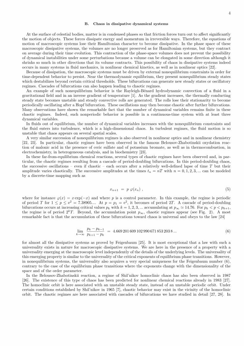
In these far-from-equilibrium chemical reactions, several types of chaotic regimes have been observed and, in par-ticular, the chaotic regimes resulting from a cascade of period-doubling bifurcations. In this period-doubling chaos,the successive oscillations – even if chaotic – each occurs after a relatively well-defined lapse of time T but theiramplitude varies chaotically. The successive amplitudes at the times tn = nT with n = 0, 1, 2, 3, ... can be modeledby a discrete-time mapping such as

xn+1 = p ϕ(xn) , (5)

where for instance ϕ(x) = x exp(−x) and where p is a control parameter. In this example, the regime is periodicof period T for 1 ≤ p ≤ e2 = 7.38905.... At p = p1 = e2, it becomes of period 2T . A cascade of period-doublingbifurcations occurs at increasing critical values pk with k = 1, 2, 3, ... accumulating at p∞ ' 14.76. For pk < p < pk+1,the regime is of period 2kT . Beyond, the accumulation point p∞, chaotic regimes appear (see Fig. 2). A mostremarkable fact is that the accumulation of these bifurcations toward chaos is universal and obeys to the law [24]

limk→∞

pk − pk−1

pk+1 − pk= 4.669 201 609 102 990 671 853 203 8 ... (6)

for almost all the dissipative systems as proved by Feigenbaum [25]. It is most exceptional that a law with such auniversality exists in nature for macroscopic dissipative systems. We are here in the presence of a property with auniversality emerging at the macroscopic level independently of the details of the underlying levels. The universality ofthis emerging property is similar to the universality of the critical exponents of equilibrium phase transitions. However,in nonequilibrium systems, the universality also acquires a very special uniqueness for the Feigenbaum number (6),contrary to the case of the equilibrium phase transitions where the exponents change with the dimensionality of thespace and of the order parameter.

In the Belousov-Zhabotinskii reaction, a regime of Shil’nikov homoclinic chaos has also been observed in 1987[26]. The existence of this type of chaos has been predicted for nonlinear chemical reactions already in 1983 [27].The homoclinic orbit is here associated with an unstable steady state, instead of an unstable periodic orbit. Undercertain conditions established by Shil’nikov in 1965 [7], chaotic behavior may exist in the vicinity of the homoclinicorbit. The chaotic regimes are here associated with cascades of bifurcations we have studied in detail [27, 28]. In

5

0

1

2

3

4

5

6

7

8

0 5 10 15 20

x

p

(a)

-1

0

10 5 10 15 20

λ+

(b)

FIG. 2: (a) Distortion of the attractor of the one-dimensional mapping (5) under changes of the control parameter p. (b) ItsLyapunov exponent λ+ versus p. The regime is chaotic when the Lyapunov exponent is positive.

homoclinic chaos, the oscillations are composed of small amplitudes around the unstable steady state and of largeamplitudes along the homoclinic loop. Homoclinic chaos has been observed in the Belousov-Zhabotinskii reaction[26], in electrochemistry [29], in fluid mechanics [30], and in nonlinear optics [31].

In the aforementioned chaotic regimes, the chaos is characterized by a single positive Lyapunov exponent so thatdynamics only involves a small number of undamped dynamical variables in such regimes.

III. CHAOS AND FRACTALS

Benoıt Mandelbrot introduced the concept of fractals which are self-similar objects with a non-integer dimensionin general [32]. In the context of dynamical systems, this fractal dimension can be used in order to give a precisemeaning to the notion of the number of undamped dynamical variables.

A. Fractal repeller and chaotic scattering

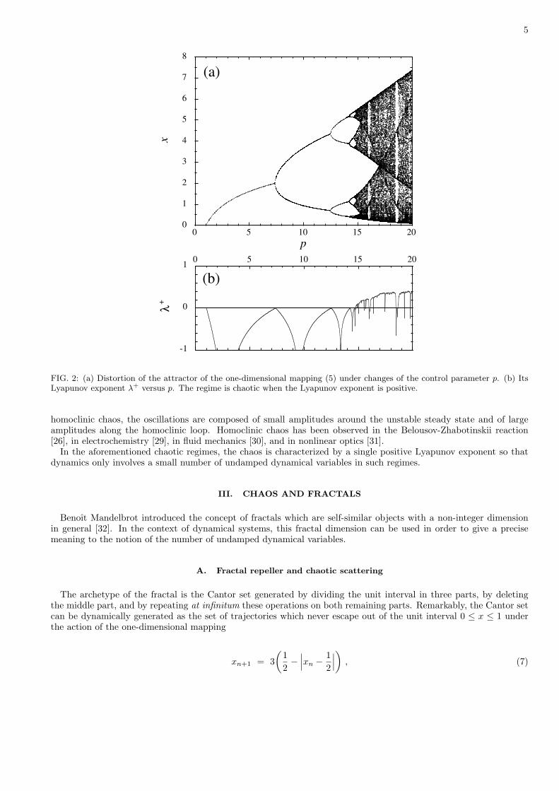
The archetype of the fractal is the Cantor set generated by dividing the unit interval in three parts, by deletingthe middle part, and by repeating at infinitum these operations on both remaining parts. Remarkably, the Cantor setcan be dynamically generated as the set of trajectories which never escape out of the unit interval 0 ≤ x ≤ 1 underthe action of the one-dimensional mapping

xn+1 = 3(

12−∣∣∣xn − 1

2

∣∣∣) , (7)

6

depiced in Fig. 3a. Indeed, most of the trajectories escape out of the unit interval through the opening 1/3 < x < 2/3,and only a Cantor set of trajectories remain trapped inside the unit interval (see Fig. 3b). These trapped trajectoriesform an invariant set which is mapped onto itself under the dynamics. Their Lyapunov exponent is λ+ = ln 3, whilethe KS entropy per iteration for the dynamics on the Cantor set is equal to hKS = ln 2. The ratio between the KSentropy and the Lyapunov exponent defines the so-called information dimension which, in this case of a uniformlyexpanding map, is equal to the Hausdorff dimension of the invariant set [10]

dI =hKS

λ+=

ln 2ln 3

= dH . (8)

The non-integer value of this dimension shows that the Cantor set forms a fractal invariant set for the one-dimensionalmapping (7). Since most trajectories escape from the vicinity of this set, it is called a fractal repeller [33].

0

1

0 1

xn+

1

xn

(a)

0

2

4

6

8

0 0.2 0.4 0.6 0.8 1

Tesc

x

(b)

FIG. 3: (a) First return plot of the one-dimensional mapping (7). (b) Time taken by a trajectory to escape out of the unitinterval under the dynamics of the mapping (7) versus the initial condition of the trajectory. We observe that this escape timevaries in an extremely complex way and that it becomes infinite for each initial condition taken on the Cantor set of trappedtrajectories.

Fractal repellers also exist in higher-dimensional systems. For a two-dimensional mapping with a positive λ+ > 0and a negative λ− < 0 Lyapunov exponents such as the Smale horseshoe map [8], the repeller is fractal not only alongthe unstable direction associated with λ+ but also in the stable direction associated with λ−. Therefore, we find twopartial information dimensions, one for each direction: d+ = hKS/λ

+ and d− = hKS/|λ−|. The total informationdimension of the fractal repeller in the two-dimensional phase space is thus the sum of both

D(2)I = d+ + d− =

hKS

λ++hKS

|λ−|, (9)

a formula proved by Young [34].In still higher-dimensional systems, partial information dimensions d+

i can be defined associated to each positive λ+i

(and negative) Lyapunov exponents. Introducing the partial information codimensions c+i = 1− d+i , the KS entropy

and the escape rate are given by [10]

hKS =∑i

d+i λ+

i , (10)

γ =∑i

λ+i − hKS =

∑i

(1− d+i ) λ+

i =∑i

c+i λ+i , (11)

leading to the interpretations of d+i λ

+i as partial entropies and of c+i λ

+i as partial escape rates characterizing the

escape in each unstable direction associated with a certain positive Lyapunov exponent λ+i .

7

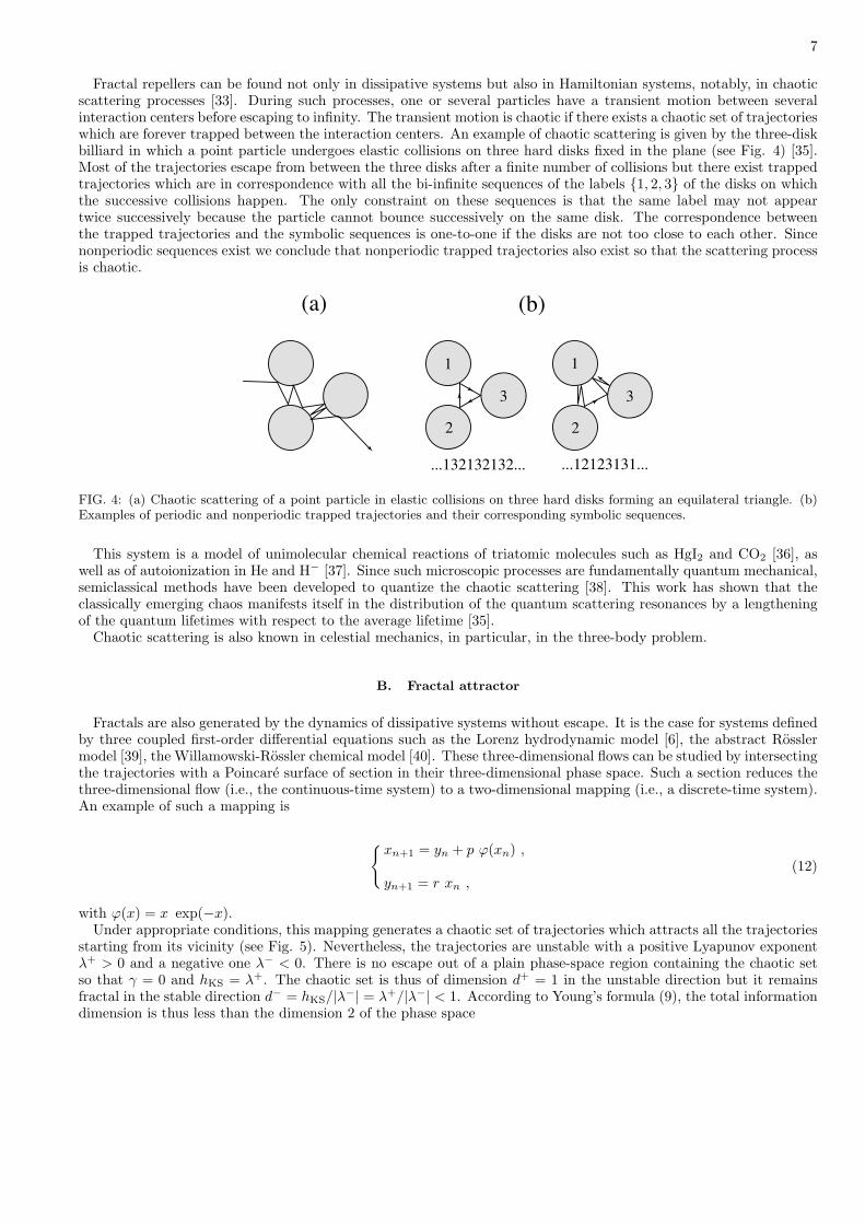
Fractal repellers can be found not only in dissipative systems but also in Hamiltonian systems, notably, in chaoticscattering processes [33]. During such processes, one or several particles have a transient motion between severalinteraction centers before escaping to infinity. The transient motion is chaotic if there exists a chaotic set of trajectorieswhich are forever trapped between the interaction centers. An example of chaotic scattering is given by the three-diskbilliard in which a point particle undergoes elastic collisions on three hard disks fixed in the plane (see Fig. 4) [35].Most of the trajectories escape from between the three disks after a finite number of collisions but there exist trappedtrajectories which are in correspondence with all the bi-infinite sequences of the labels {1, 2, 3} of the disks on whichthe successive collisions happen. The only constraint on these sequences is that the same label may not appeartwice successively because the particle cannot bounce successively on the same disk. The correspondence betweenthe trapped trajectories and the symbolic sequences is one-to-one if the disks are not too close to each other. Sincenonperiodic sequences exist we conclude that nonperiodic trapped trajectories also exist so that the scattering processis chaotic.

1

2

3

1

2

3

...132132132... ...12123131...

(a) (b)

FIG. 4: (a) Chaotic scattering of a point particle in elastic collisions on three hard disks forming an equilateral triangle. (b)Examples of periodic and nonperiodic trapped trajectories and their corresponding symbolic sequences.

This system is a model of unimolecular chemical reactions of triatomic molecules such as HgI2 and CO2 [36], aswell as of autoionization in He and H− [37]. Since such microscopic processes are fundamentally quantum mechanical,semiclassical methods have been developed to quantize the chaotic scattering [38]. This work has shown that theclassically emerging chaos manifests itself in the distribution of the quantum scattering resonances by a lengtheningof the quantum lifetimes with respect to the average lifetime [35].

Chaotic scattering is also known in celestial mechanics, in particular, in the three-body problem.

B. Fractal attractor

Fractals are also generated by the dynamics of dissipative systems without escape. It is the case for systems definedby three coupled first-order differential equations such as the Lorenz hydrodynamic model [6], the abstract Rosslermodel [39], the Willamowski-Rossler chemical model [40]. These three-dimensional flows can be studied by intersectingthe trajectories with a Poincare surface of section in their three-dimensional phase space. Such a section reduces thethree-dimensional flow (i.e., the continuous-time system) to a two-dimensional mapping (i.e., a discrete-time system).An example of such a mapping is

{xn+1 = yn + p ϕ(xn) ,

yn+1 = r xn ,(12)

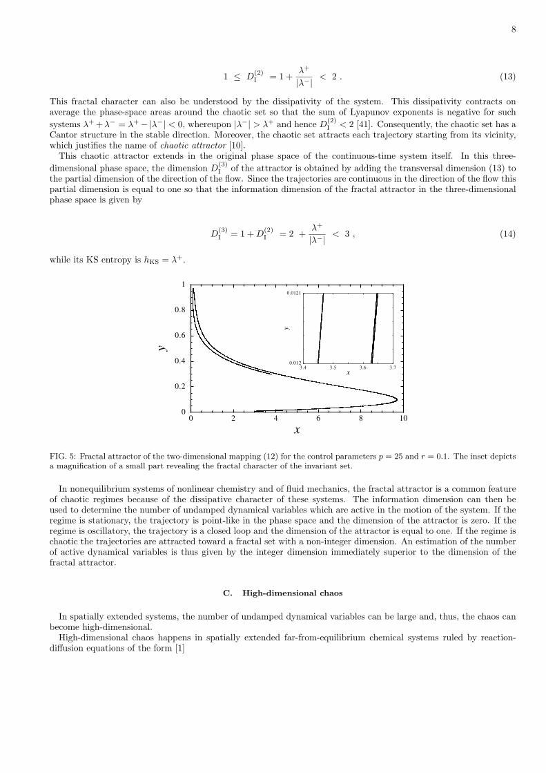
with ϕ(x) = x exp(−x).Under appropriate conditions, this mapping generates a chaotic set of trajectories which attracts all the trajectories

starting from its vicinity (see Fig. 5). Nevertheless, the trajectories are unstable with a positive Lyapunov exponentλ+ > 0 and a negative one λ− < 0. There is no escape out of a plain phase-space region containing the chaotic setso that γ = 0 and hKS = λ+. The chaotic set is thus of dimension d+ = 1 in the unstable direction but it remainsfractal in the stable direction d− = hKS/|λ−| = λ+/|λ−| < 1. According to Young’s formula (9), the total informationdimension is thus less than the dimension 2 of the phase space

8

1 ≤ D(2)I = 1 +

λ+

|λ−|< 2 . (13)

This fractal character can also be understood by the dissipativity of the system. This dissipativity contracts onaverage the phase-space areas around the chaotic set so that the sum of Lyapunov exponents is negative for suchsystems λ+ +λ− = λ+−|λ−| < 0, whereupon |λ−| > λ+ and hence D(2)

I < 2 [41]. Consequently, the chaotic set has aCantor structure in the stable direction. Moreover, the chaotic set attracts each trajectory starting from its vicinity,which justifies the name of chaotic attractor [10].

This chaotic attractor extends in the original phase space of the continuous-time system itself. In this three-dimensional phase space, the dimension D(3)

I of the attractor is obtained by adding the transversal dimension (13) tothe partial dimension of the direction of the flow. Since the trajectories are continuous in the direction of the flow thispartial dimension is equal to one so that the information dimension of the fractal attractor in the three-dimensionalphase space is given by

D(3)I = 1 +D

(2)I = 2 +

λ+

|λ−|< 3 , (14)

while its KS entropy is hKS = λ+.

0

0.2

0.4

0.6

0.8

1

0 2 4 6 8 10

y

x

0.012

0.0121

3.4 3.5 3.6 3.7

y

x

FIG. 5: Fractal attractor of the two-dimensional mapping (12) for the control parameters p = 25 and r = 0.1. The inset depictsa magnification of a small part revealing the fractal character of the invariant set.

In nonequilibrium systems of nonlinear chemistry and of fluid mechanics, the fractal attractor is a common featureof chaotic regimes because of the dissipative character of these systems. The information dimension can then beused to determine the number of undamped dynamical variables which are active in the motion of the system. If theregime is stationary, the trajectory is point-like in the phase space and the dimension of the attractor is zero. If theregime is oscillatory, the trajectory is a closed loop and the dimension of the attractor is equal to one. If the regime ischaotic the trajectories are attracted toward a fractal set with a non-integer dimension. An estimation of the numberof active dynamical variables is thus given by the integer dimension immediately superior to the dimension of thefractal attractor.

C. High-dimensional chaos

In spatially extended systems, the number of undamped dynamical variables can be large and, thus, the chaos canbecome high-dimensional.

High-dimensional chaos happens in spatially extended far-from-equilibrium chemical systems ruled by reaction-diffusion equations of the form [1]

9

∂t c = F(c) + D · ∇2c (15)

where c are the concentrations of the different chemical species, F(c) are the nonlinear rates given by the mass-actionlaw, and D is the matrix of diffusion coefficients. Far-from-equilibrium, Turing-type instabilities generate stationary ornon-stationary structures in reaction-diffusion systems [1]. Such instabilities destabilize the uniform state for certaininfinitesimal perturbations δc× exp(ik · r− iωt). The dispersion relation of these perturbations is [1]

−i ω δc =

(∂F∂c

− k2 D

)· δc . (16)

As shown by Nicolis and coworkers [42, 43], the range of wavenumbers which become unstable is of the order

k0 ∼∥∥∥D−1 · ∂F

∂c

∥∥∥1/2

∼ 1`0

, (17)

where ‖ · ‖ denotes the Euclidian or the maximum norm of the matrix. The range (17) is of the order of the inverseof the smallest structures appearing in the system beyond the instability. A remakable feature is that the scale `0 isintrinsic to the reaction-diffusion system and to its nonlinear chemistry.

A typical positive Lyapunov exponent has a value of the order of the imaginary frequency of Eq. (16) in the middleof the range (17) [44]:

λ+ ∼∥∥∥∂F∂c

∥∥∥ . (18)

The information dimension of the fractal attractor can then be estimated as the total number of the structures of size`0 inside the total volume Ld of the d-dimensional system [44]:

DI ∼(L

`0

)d∼ Ld

∥∥∥D−1 · ∂F∂c

∥∥∥d/2 . (19)

The Kolmogorov-Sinai entropy per unit time, which is given by the sum of positive Lyapunov exponents hKS =∑i λ

+i ,

is then of the following order

hKS ∼ DI λ+ ∼ Ld

∥∥∥D−1 · ∂F∂c

∥∥∥d/2 ∥∥∥∂F∂c

∥∥∥ . (20)

This high-dimensional chaos which appears in spatially extended systems is known as spatio-temporal chaos and ithas been observed in many different contexts [1].

Another example of high-dimensional chaos is turbulence. For a turbulent incompressible fluid described by theNavier-Stokes equations

∂t v + v · ∇v = − 1ρ ∇P + ν ∇2v ,

∇ · v = 0 ,(21)

the information dimension of its fractal attractor can be estimated by using Kolmogorov’s theory of turbulence [45].The fluid is supposed to be driven by nonequilibrium constraints on a large spatial scale L where the constraintsgenerate a motion of velocity V . This large-scale motion is broken into small-scale motions because of the convectiveinstability which repeats itself in a cascade down to the scale where the energy dissipation damps convection. If εis the energy dissipated per unit time and per unit mass of the fluid and if ν is the kinematic viscosity in m2/s, thedissipation scale is given by forming a quantity with the unit of a length from ε and ν, which is

`0 ∼(ν3

ε

)1/4

. (22)

10

Similarly, a dissipation time can be defined as t0 ∼ `20/ν ∼ (ν/ε)1/2. On the intermediate length scales ` betweenthe large one L and the small one `0, a Kolmogorov cascade is generated by the convection instability. Energy isconserved in this cascade for L > ` > `0, but energy is transferred from the large scale L down to the smallest scale`0 where it is dissipated. The dissipated energy ε is a quantity which is invariant in the cascade so that it is equal tothe energy introduced at its top by the nonequilibrium constraints so that ε ∼ V 3/L.

An estimation of the information dimension is given by the number of cells with the size of the dissipation length(22) in the fluid, i.e.,

DI ∼

(L

`0

)3

∼ ε3/4

ν9/4L3 . (23)

Similarly, a typical positive Lyapunov exponent is estimated by the inverse of the dissipation time

λ+ ∼ t−10 ∼

(ε

ν

)1/2

. (24)

The KS entropy is thus estimated as being the order of magnitude of the information dimension (23) multiplied bythe value (24) of a typical positive Lyapunov exponent

hKS ∼ DI λ+ ∼ ε5/4

ν11/4L3 . (25)

If we introduce the dimensionless Reynold number

R def=L V

ν, (27)

we get that

DI ∼ R9/4 ,

λ+ ∼ R1/2 VL ,

hKS ∼ R11/4 VL ,

(28)

up to dimensionless numerical constants. The conclusion is that the dimension of the fractal attractor increases asthe power 9/4 of the Reynolds number. Rigorous estimates confirm this result [46]. As a consequence, the numberof active dynamical variables may be very large in turbulent regimes. From this viewpoint, turbulence appears asa high-dimensional chaos, while the chaotic regimes generated immediately after the destabilization of periodic (orquasiperiodic) regimes are referred to as low-dimensional chaos.

Since the turbulent regimes are very common, this high-dimensional macroscopic chaos is a problem of majorpreoccupation in the study of planetary and stellar atmospheres as well as in the Earth hydrosphere. In particular,low- and high-dimensional chaos have been studied in meteorology in order to characterize the predicitability ofmeteorological forecasts [47]. In this context, the concept of Lyapunov exponent has become of major importance fordetermining the time horizon within which a reliable prediction can be performed [47].

High-dimensional chaos also exists in magnetohydrodynamics, in plasmas, and in nonlinear optics.If the dimension of the attractor is very high and if the dynamics evolves on several scales, the smallest scales

generate in general a very fast chaos which drives the larger scales by fluctuating forces similar to noises. In suchcases, the dynamics can be modeled as a stochastic process. (Examples of stochastic processes which are referred tohere are Brownian motion, the Langevin process, the Ornstein-Uhlenbeck process, Mandelbrot’s fractional Brownianmotion, the Yaglom noises, etc...) In this perspective, if the underlying system is deterministic, the stochastic processesturn out to be high-dimensional chaos [33].

11

D. Instabilites and self-similar disordered structures

We can imagine that spatially disordered structures can be generated in a spatially extended chaotic system whichslows down for instance because of cooling. Similarly, small-scale instabilities in a growth process can generateirregular and dendritic structures. Such spatially disordered structures are found in transport problems in porousmedia, random networks or hydrological systems [48–51], in growth phenomena such as diffusion-limited aggregations[51–53], in the formation of nanostructures on surfaces [54], in biological growth phenomena, etc ... On certainscales, such structures often display self-similar properties which can be characterized by scaling exponents such asfractal dimensions. New methods have been developed in order to understand the scaling laws which rule these largeheterogeneous structures [48–54].

Such self-similar structures are generated by some mechanisms of instability but the scaling laws can often beestablished by the global properties of the system such as the conservation laws. An example is the aforementionedKolmogorov cascade in turbulence.

Another example is the formation of gravitational structures in self-graviting systems such as interstellar clouds[55]. Numerous observations show that mass is not distributed uniformly in astrophysical systems. If it was thecase, Sun-like stars would be uniformly distributed in space, the sky at night would be as bright as the Sun, and nocool reservoir would exist for the thermodynamic machines to work on Earth. However, we remark that the celestialbodies interact through the gravitational force which has the peculiarity to be attractive and long ranged. The absenceof repulsive short-ranged forces is at the origin of the instability of the uniform distributions of matter, as alreadyshown by Jeans. It is worthwhile to revisit the Jeans instability in the light of modern dynamical systems theory. Aself-graviting fluid can be described as a dynamical system ruled by the following dissipativeless equations:

∂t v + v · ∇v = − 1

ρ ∇P −∇φ ,

∂t ρ+∇ · (ρv) = 0 ,

∇2φ = 4πGρ ,

(29)

where φ is the gravitational potential and G the gravitational constant. The total energy

E =∫ρ

(12

v2 + u

)dr − G

∫dr dr′

ρ(r) ρ(r′)‖r− r′‖

, (30)

is conserved in this system (where u is the internal energy per unit mass of the fluid). The stability of a static fluid ofdensity ρ0, pressure P0 and vanishing velocity v0 = 0 can be analyzed by linearizing Eqs. (29), assuming ρ = ρ0 + ρ1,v = v1 and P = P0 + v2

s ρ1 where vs = (∂P/∂ρ)1/2adiabatic is the sound velocity. The linearization leads to the equation[56]:

∂2t ρ1 = v2

s ∇2ρ1 + 4πGρ0 ρ1 . (31)

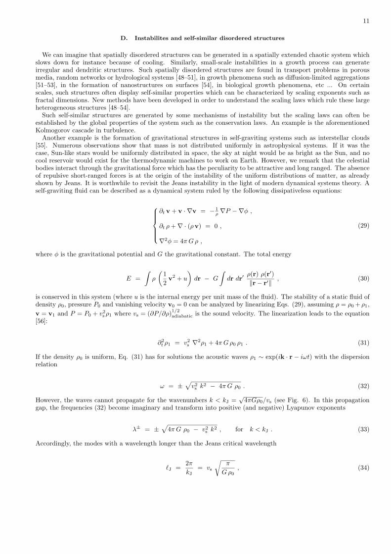
If the density ρ0 is uniform, Eq. (31) has for solutions the acoustic waves ρ1 ∼ exp(ik · r − iωt) with the dispersionrelation

ω = ±√v2s k

2 − 4πG ρ0 . (32)

However, the waves cannot propagate for the wavenumbers k < kJ =√

4πGρ0/vs (see Fig. 6). In this propagationgap, the frequencies (32) become imaginary and transform into positive (and negative) Lyapunov exponents

λ± = ±√

4πG ρ0 − v2s k

2 , for k < kJ . (33)

Accordingly, the modes with a wavelength longer than the Jeans critical wavelength

`J =2πkJ

= vs

√π

Gρ0, (34)

12

0

0k

k+k

J−k

J

λ

ω

FIG. 6: The upper plot depicts the dispersion relation given by Eq. (32) and the lower one the positive Lyapunov exponentsgiven by Eq. (33) for acoustic waves of wavenumber k in a uniformly distributed self-graviting fluid. The dashed diagonal linesare the asymptotes ω ≈ vsk and kJ is the Jeans critical wavenumber.

are all unstable and grow until the nonlinearities enter into play. This Jeans instability leads to the collapse of spatiallyextended uniformly distributed self-graviting fluids, which is a well-known phenomenon occurring for instance in theformation of stars inside the interstellar clouds.

The Jeans instability is at the origin of the formation of large-scale structures in self-graviting systems, as shownby the following discussion. In many systems, the sound velocity is of the order of the velocity of the particles whichcompose the system. If we consider a self-graviting system on the scale R, the velocities of the particles are expectedto be statistically distributed around an average v(R) ∼ vs, which depends in general on the scale R considered.The total mass on the scale R is related to the scale-dependent density ρ(R) according to M(R) = 4πR3ρ(R)/3.Gravitational structures can be conceived as being hierarchical and dynamical with the Jeans instability occurring oneach scale. Accordingly, the Jeans wavelength (34) corresponding to the density ρ0 ∼ ρ(R) is expected to be of theorder of the scale itself, R ∼ `J, from which we obtain the estimation

v(R) ∼√GM(R)

R. (35)

On the other hand, the energy of a subsystem of size R is estimated according to Eqs. (30) and (35) to be of theorder of

E(R) ∼ − GM(R)2

R. (36)

If we assume that the energy tends to be uniformly distributed by the dynamics of the total system, this energy shouldscale like E(R) ∼ R3. This assumption is based on the idea that the system has reached a dynamical quasi-equilibriumduring its previous time evolution so that the chemical potential is approximately the same for each of its parts [57].As a consequence of this assumption, the mass and the velocity should scale as

13

M(R) ∼ R2 ,

v(R) ∼√R ,

(37)

which are close to the scaling exponents observed in self-graviting systems [55]. Accordingly, the mass tends toevolve toward a two-dimensional distribution, which is possibly “fractal”, instead of the uniform three-dimensionaldistribution expected in systems with repulsive short-ranged interactions. In conclusion, the long-ranged attractivegravitational interaction precludes an equilibrium uniform distribution of matter in self-graviting systems and, instead,leads to heterogeneous self-similar structures generated by the Jeans instability.

This result that an instability is at the basis of the formation of structures – and especially of fractal structures –seems to be of a great generality, not only in macroscopic systems but also in microscopic ones as discussed below.

IV. MICROSCOPIC CHAOS

At the microscopic level, a fluid is composed of particles undergoing endless mutual collisions. A very ancient modelgoing back to Bernoulli depicts a fluid as a dynamical system of small hard spheres in elastic collisions. This systemcaptures some of the main properties of a gas at room temperature and it continues to be intensively studied, inparticular, to determine its chaotic properties.

A. Instability and collisional chaos

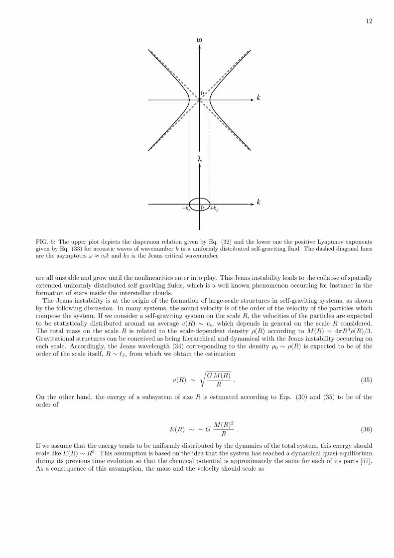
The defocusing character of an elastic collision between two hard spheres suggests that the hard-sphere gas is highlyunstable and chaotic. The role of this dynamical instability in the relaxation of the fluid toward the thermodynamicequilibrium has been already discussed by Krylov more than fifty years ago [58]. However, only recent work has shownin detail the relationship between the microscopic chaos and the relaxation toward the thermodynamic equilibrium[33].

δα

δα'

FIG. 7: Geometry of a collision between two particles and of the growth of a perturbation on the velocity of a particle: δα→ δα′.

In this context, the concepts of Lyapunov exponent and KS entropy have been seriously considered only recentlyand the quantitative evaluation of these quantities for a gas of particles at room temperature has been carried outonly since 1985 [59, 60]. The order of magnitude of a typical Lyapunov exponent is determined by the diameter d ofthe particles, by their mean free path `, and by their average velocity v. The mean free path is given by the diameterd and by the density n of the particles according to ` ∼ 1/(nd2). The mean velocity is a function of the temperatureT , of the mass m of the particles, and of the Boltzmann constant kB: v ∼

√kBT/m. A typical Lyapunov exponent

can be estimated by observing that a perturbation on the velocity of a particle increases significantly after collision onanother particle (see Fig. 7). If δα is the angle between the reference and perturbed trajectories, this angle increasesby a factor `/d after the collision. If τ ∼ `/v is the mean intercollisional time, the angle of the perturbation willincrease by the factor (`/d)t/τ after a time t. The growth of the perturbation is thus exponential and characterizedby the positive Lyapunov exponent [59]:

14

λ+ ∼ v

`ln`

d. (38)

There are as many positive Lyapunov exponents as there are unstable directions in the phase space of the N -particlesystem. For a mole of particles, the number of positive Lyapunov exponents is thus of the order of the Avogadronumber NAv ' 6× 1023. As a consequence, the KS entropy per unit time is of the order of [59]

hKS ∼ N λ+ , with N ∼ NAv . (39)

Since the system is Hamiltonian, the phase-space volumes are preserved by the dynamics and no fractal attractor ispossible. The dimension of the system is thus equal to the dimension of the hypersurface of constant energy H = E(also called the energy shell) if the gas is isolated in a heavy Dewar bottle: DI = 6N − 1.

0.001

0.01

0.1

0 32 64 96 128

DB = 5

DB = 25

DB = 50

DB = 100

DB = 250

λi

i

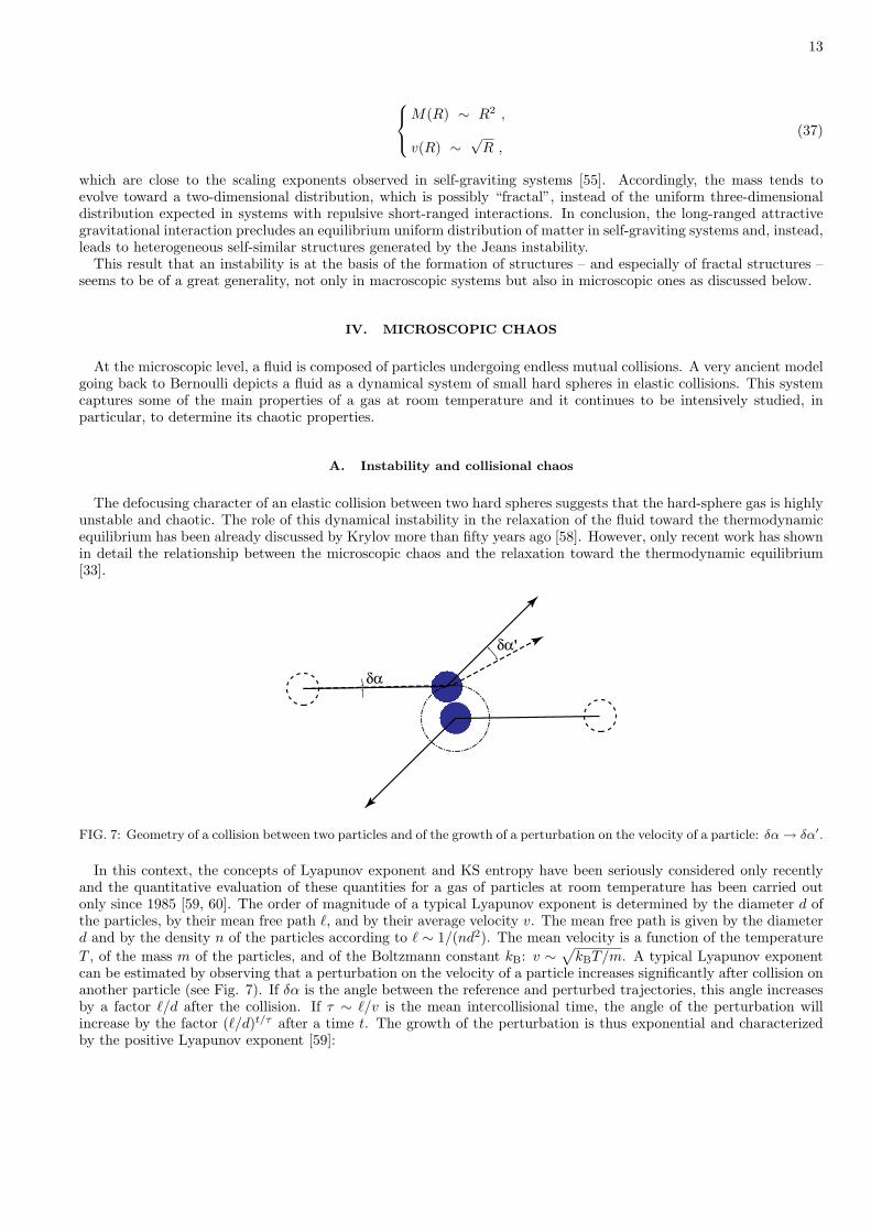
FIG. 8: Spectrum of positive Lyapunov exponents for a system of one hard disk of diameter DB and of 63 hard disks of unitdiameter. The density of the surrounding fluid is here n = 10−3 [61]. The Lyapunov exponents increase with the diameter DB

of the Brownian particle.

The microscopic chaos is fundamentally different from the macroscopic chaos described in the previous section. In-deed, there is no macroscopic chaos in a fluid at the thermodynamic equilibrium. Nevertheless, an intense microscopicchaos animates the motion of the particles composing this fluid.

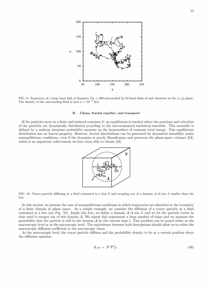
The microscopic chaos manifests itself in different random processes due to the thermal fluctuations such as theBrownian motion of a colloidal particle. Figure 8 depicts the spectrum of the positive Lyapunov exponents of amodel of Brownian motion in which a large disk undergoes elastic collisions with a surrounding fluid of small harddisks. The area below the spectrum of the Lyapunov exponents gives the KS entropy which is the total amount ofdynamical randomness developed by the full system. This huge dynamical randomness appears to be at the origin ofthe erratic motion of the colloidal particle seen in Fig. 9 [61]. In this new interpretation which have also been studiedexperimentally [62], Brownian motion results from the high-dimensional chaos of the surrounding fluid.

In this perspective, the new quantities such as the KS entropy per unit time or the Lyapunov exponents provide theway to establish quantitative comparisons between the chaos in the microscopic Newtonian dynamics of the particlesand the dynamical randomness which is traditionally understood in terms of stochastic models. It should be pointedout that the dynamical randomness is defined a priori in the stochastic models which, therefore, do not explain butassume this property. The new results reinterpret these stochastic processes in terms of a high-dimensional chaos inthe microscopic Newtonian dynamics, thus providing an explanation of the observed dynamical randomness.

15

0

50

100

150

200

50 100 150 200 250

y

x

FIG. 9: Trajectory of a large hard disk of diameter DB = 300 surrounded by 63 hard disks of unit diameter in the (x, y) plane.The density of the surrounding fluid is here n = 10−3 [61].

B. Chaos, fractal repeller, and transport

If the particles move in a finite and isolated container V, an equilibrium is reached where the positions and velocitiesof the particles are dynamically distributed according to the microcanonical statistical ensemble. This ensemble isdefined by a uniform invariant probability measure on the hypersurface of constant total energy. This equilibriumdistribution has no fractal property. However, fractal distributions can be generated by dynamical instability undernonequilibrium conditions, even if the dynamics is purely Hamiltonian and preserves the phase-space volumes [63],which is an important achievement we have been able to obtain [33].

L

V

A

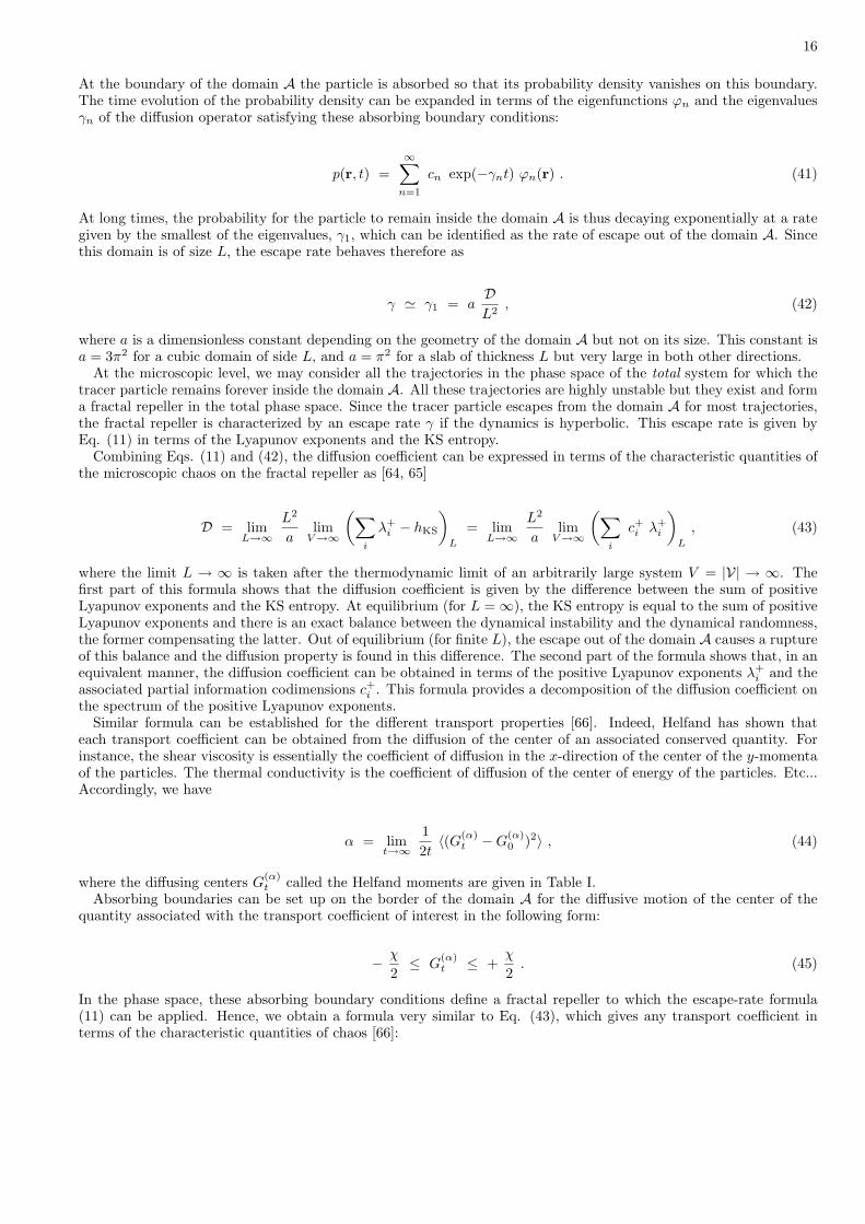
FIG. 10: Tracer particle diffusing in a fluid contained in a box V and escaping out of a domain A of size L smaller than thebox.

In this section, we present the case of nonequilibrium conditions in which trajectories are absorbed at the boundaryof a finite domain in phase space. As a simple example, we consider the diffusion of a tracer particle in a fluidcontained in a box (see Fig. 10). Inside this box, we define a domain A of size L and we let the particle evolve intime until it escapes out of this domain A. We repeat this experiment a large number of times and we measure theprobability that the particle is still in the domain A by the current time t. This problem can be posed either at themacroscopic level or at the microscopic level. The equivalence between both descriptions should allow us to relate themacroscopic diffusion coefficient to the microscopic chaos.

At the macroscopic level, the tracer particle diffuses and the probability density to be at a certain position obeysthe diffusion equation

∂t p = D ∇2p . (40)

16

At the boundary of the domain A the particle is absorbed so that its probability density vanishes on this boundary.The time evolution of the probability density can be expanded in terms of the eigenfunctions ϕn and the eigenvaluesγn of the diffusion operator satisfying these absorbing boundary conditions:

p(r, t) =∞∑n=1

cn exp(−γnt) ϕn(r) . (41)

At long times, the probability for the particle to remain inside the domain A is thus decaying exponentially at a rategiven by the smallest of the eigenvalues, γ1, which can be identified as the rate of escape out of the domain A. Sincethis domain is of size L, the escape rate behaves therefore as

γ ' γ1 = aDL2

, (42)

where a is a dimensionless constant depending on the geometry of the domain A but not on its size. This constant isa = 3π2 for a cubic domain of side L, and a = π2 for a slab of thickness L but very large in both other directions.

At the microscopic level, we may consider all the trajectories in the phase space of the total system for which thetracer particle remains forever inside the domain A. All these trajectories are highly unstable but they exist and forma fractal repeller in the total phase space. Since the tracer particle escapes from the domain A for most trajectories,the fractal repeller is characterized by an escape rate γ if the dynamics is hyperbolic. This escape rate is given byEq. (11) in terms of the Lyapunov exponents and the KS entropy.

Combining Eqs. (11) and (42), the diffusion coefficient can be expressed in terms of the characteristic quantities ofthe microscopic chaos on the fractal repeller as [64, 65]

D = limL→∞

L2

alimV→∞

(∑i

λ+i − hKS

)L

= limL→∞

L2

alimV→∞

(∑i

c+i λ+i

)L

, (43)

where the limit L → ∞ is taken after the thermodynamic limit of an arbitrarily large system V = |V| → ∞. Thefirst part of this formula shows that the diffusion coefficient is given by the difference between the sum of positiveLyapunov exponents and the KS entropy. At equilibrium (for L = ∞), the KS entropy is equal to the sum of positiveLyapunov exponents and there is an exact balance between the dynamical instability and the dynamical randomness,the former compensating the latter. Out of equilibrium (for finite L), the escape out of the domain A causes a ruptureof this balance and the diffusion property is found in this difference. The second part of the formula shows that, in anequivalent manner, the diffusion coefficient can be obtained in terms of the positive Lyapunov exponents λ+

i and theassociated partial information codimensions c+i . This formula provides a decomposition of the diffusion coefficient onthe spectrum of the positive Lyapunov exponents.

Similar formula can be established for the different transport properties [66]. Indeed, Helfand has shown thateach transport coefficient can be obtained from the diffusion of the center of an associated conserved quantity. Forinstance, the shear viscosity is essentially the coefficient of diffusion in the x-direction of the center of the y-momentaof the particles. The thermal conductivity is the coefficient of diffusion of the center of energy of the particles. Etc...Accordingly, we have

α = limt→∞

12t〈(G(α)

t −G(α)0 )2〉 , (44)

where the diffusing centers G(α)t called the Helfand moments are given in Table I.

Absorbing boundaries can be set up on the border of the domain A for the diffusive motion of the center of thequantity associated with the transport coefficient of interest in the following form:

− χ

2≤ G

(α)t ≤ +

χ

2. (45)

In the phase space, these absorbing boundary conditions define a fractal repeller to which the escape-rate formula(11) can be applied. Hence, we obtain a formula very similar to Eq. (43), which gives any transport coefficient interms of the characteristic quantities of chaos [66]:

17

α = limχ→∞

(χ

π

)2

limV→∞

(∑i

λ+i − hKS

)χ

= limχ→∞

(χ

π

)2

limV→∞

(∑i

c+i λ+i

)χ

. (46)

Thanks to this formula, each transport coefficient can be decomposed on the spectrum of the positive Lyapunovexponents and we could understand the contribution of each Lyapunov exponent to each transport property.

These results show the role of chaos and fractals in our understanding of irreversible transport properties such asdiffusion or viscosity.

Table I. Helfand’s moments.

process moment

self-diffusion G(D) = xi

shear viscosity G(η) = 1√V kBT

∑Ni=1 xi piy

bulk viscosity (ψ = ζ + 43η) G

(ψ) = 1√V kBT

∑Ni=1 xi pix

heat conductivity G(κ) = 1√V kBT 2

∑Ni=1 xi (Ei − 〈Ei〉)

charge conductivity G(e) = 1√V kBT

∑Ni=1 eZi xi

chemical reaction rate G(r) = 1√V kBT

(N (r) − 〈N (r)〉)

C. Chaos and relaxation to the thermodynamic equilibrium

The role of chaos appears in an even more important way in the problem of relaxation toward the equilibrium andin the second law of thermodynamics.

To illustrate the discussion, I consider the model of the Lorentz gas in which a point particle undergoes elasticcollisions on hard disks which are fixed in the plane. We suppose that the disks form a regular lattice. The Lorentzgas is a chaotic system of Hamiltonian character in which energy is conserved. Its Lyapunov exponents are λ+ > 0 >λ− = −λ+. In 1980, Bunimovich and Sinai proved [67] that, under certain conditions, the particle has a diffusivemotion on the large spatial scales, which justifies the use of the diffusion equation (40). This equation predicts theexistence of hydrodynamic modes of the form

c(r, t) ∼ exp(−Dk2t) exp(ik · r) , (47)

which are spatially periodic with the wavelength ` = 2π/k, and which decrease exponentially in time. In its timeevolution, the system approaches the thermodynamic equilibrium along these hydrodynamic modes which damp thespatial inhomogeneities of concentration. Of course, the diffusion equation (40) is only approximate and we shouldwonder whether the hydrodynamic modes exist at the microscopic level of description.

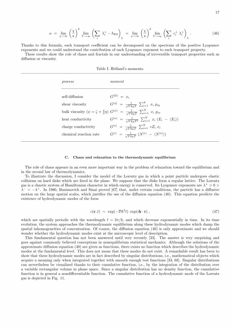
This fundamental question has not been answered until very recently [33]. The answer is very surprising andgoes against commonly believed conceptions in nonequilibrium statistical mechanics. Although the solutions of theapproximate diffusion equation (40) are given as functions, there exists no function which describes the hydrodynamicmodes at the fundamental level. This does not mean that these modes do not exist. A remarkable result has been toshow that these hydrodynamic modes are in fact described by singular distributions, i.e., mathematical objects whichacquire a meaning only when integrated together with smooth enough test functions [33, 68]. Singular distributionscan nevertheless be visualized thanks to their cumulative function, i.e., by the integration of the distribution overa variable rectangular volume in phase space. Since a singular distribution has no density function, the cumulativefunction is in general a nondifferentiable function. The cumulative function of a hydrodynamic mode of the Lorentzgas is depicted in Fig. 11.

18

-0.002

-0.001

0

0.001

0.002

-0.03

-0.02

-0.01

0

0.01

0.02

0.03

0 π/2 π 3π/2 2π

Re G

k(θ

) −

θ/2

π

Im G

k (θ

)

θ

Re

Im

FIG. 11: Real and imaginary parts of the cumulative function of a hydrodynamic mode of the periodic Lorentz gas. Theparticle moves with unit velocity. The disks have a unit radius. The distance between the centers of the disks is equal to 2.3times their radius. The wavenumbers of this hydrodynamic mode are kx = 0.1 and ky = 0.

φ. . . . . .

nn−1 n+1. . .. . .

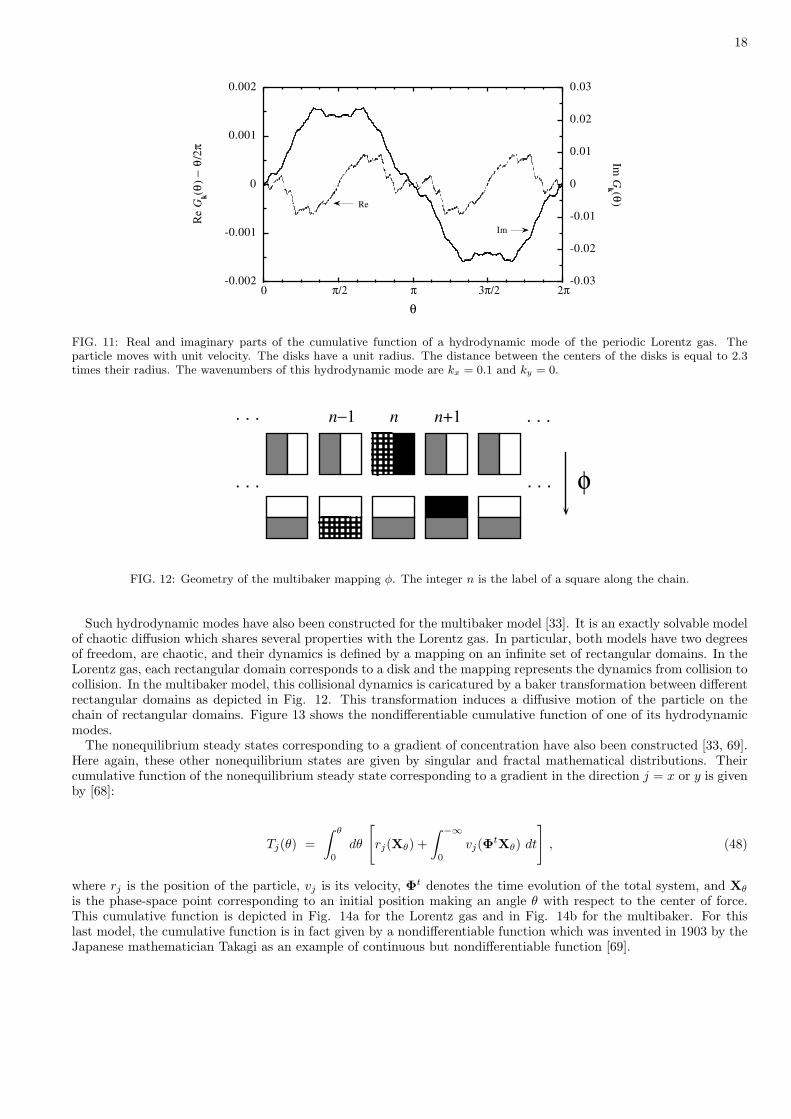
FIG. 12: Geometry of the multibaker mapping φ. The integer n is the label of a square along the chain.

Such hydrodynamic modes have also been constructed for the multibaker model [33]. It is an exactly solvable modelof chaotic diffusion which shares several properties with the Lorentz gas. In particular, both models have two degreesof freedom, are chaotic, and their dynamics is defined by a mapping on an infinite set of rectangular domains. In theLorentz gas, each rectangular domain corresponds to a disk and the mapping represents the dynamics from collision tocollision. In the multibaker model, this collisional dynamics is caricatured by a baker transformation between differentrectangular domains as depicted in Fig. 12. This transformation induces a diffusive motion of the particle on thechain of rectangular domains. Figure 13 shows the nondifferentiable cumulative function of one of its hydrodynamicmodes.

The nonequilibrium steady states corresponding to a gradient of concentration have also been constructed [33, 69].Here again, these other nonequilibrium states are given by singular and fractal mathematical distributions. Theircumulative function of the nonequilibrium steady state corresponding to a gradient in the direction j = x or y is givenby [68]:

Tj(θ) =∫ θ

0

dθ

[rj(Xθ) +

∫ −∞

0

vj(ΦtXθ) dt

], (48)

where rj is the position of the particle, vj is its velocity, Φt denotes the time evolution of the total system, and Xθ

is the phase-space point corresponding to an initial position making an angle θ with respect to the center of force.This cumulative function is depicted in Fig. 14a for the Lorentz gas and in Fig. 14b for the multibaker. For thislast model, the cumulative function is in fact given by a nondifferentiable function which was invented in 1903 by theJapanese mathematician Takagi as an example of continuous but nondifferentiable function [69].

19

-0.3

-0.2

-0.1

0

0.1

0.2

0.3

-0.1

0

0.1

0.2

0.3

0.4

0.5

0 0.2 0.4 0.6 0.8 1

Re G

k(y

) −

y Im G

k (y)

y

Re Im

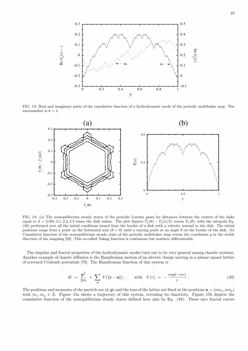
FIG. 13: Real and imaginary parts of the cumulative function of a hydrodynamic mode of the periodic multibaker map. Thewavenumber is k = 1.

-0.3

-0.2

-0.1

0

0.1

0.2

0.3

-0.3 -0.2 -0.1 0 0.1 0.2 0.3

Ty(θ

) −

Ty(π

/2)

Tx(θ)

0

0.4

0.8

0 0.5 1

T(y

)

y

(a) (b)

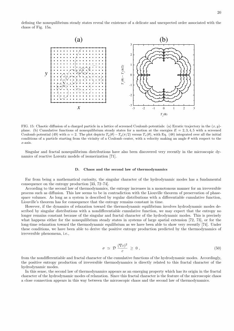
FIG. 14: (a) The nonequilibrium steady states of the periodic Lorentz gases for distances between the centers of the disksequal to d = 2.001, 2.1, 2.2, 2.3 times the disk radius. The plot depicts Ty(θ) − Ty(π/2) versus Tx(θ), with the integrals Eq.(48) performed over all the initial conditions issued from the border of a disk with a velocity normal to the disk. The initialpositions range from a point on the horizontal axis (θ = 0) until a varying point at an angle θ on the border of the disk. (b)Cumulative function of the nonequilibrium steady state of the periodic multibaker map versus the coordinate y in the stabledirection of the mapping [69]. This so-called Takagi function is continuous but nowhere differentiable.

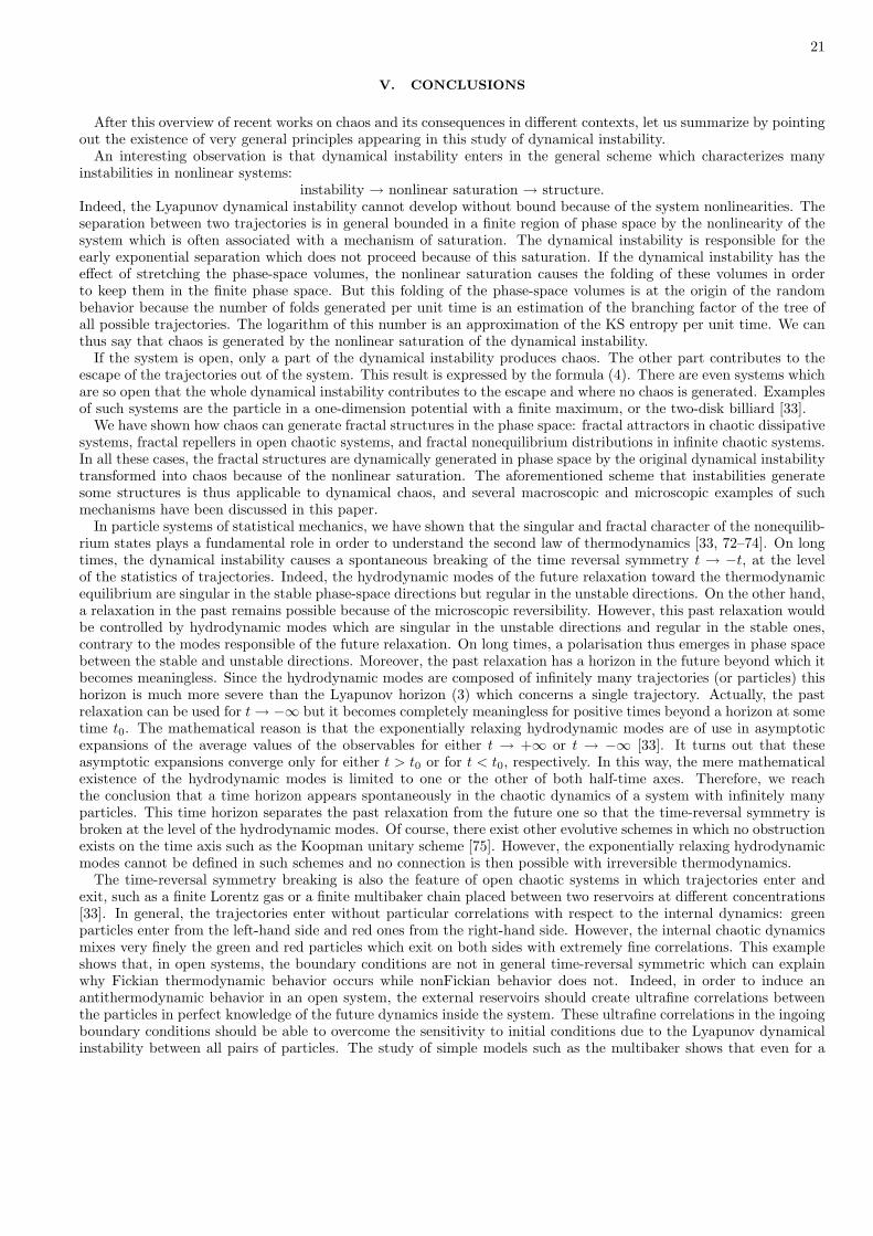
The singular and fractal properties of the hydrodynamic modes turn out to be very general among chaotic systems.Another example of chaotic diffusion is the Hamiltonian motion of an electric charge moving in a planar square latticeof screened Coulomb potentials [70]. The Hamiltonian function of this system is

H =p2

2m+∑a

V (‖r− a‖) , with V (r) = − exp(−αr)r

. (49)

The positions and momenta of the particle are (r,p) and the ions of the lattice are fixed at the positions a = (amx, amy)with mx,my ∈ Z. Figure 15a shows a trajectory of this system, revealing its chaoticity. Figure 15b depicts thecumulative function of the nonequilibrium steady states defined here also by Eq. (48). These nice fractal curves

20

defining the nonequilibrium steady states reveal the existence of a delicate and unexpected order associated with thechaos of Fig. 15a.

-3

-2

-1

0

1

2

3

-3 -2 -1 0 1 2 3

Ty(θ

) −

Ty(π

/2)

Tx(θ)

(a) (b)

x

y

FIG. 15: Chaotic diffusion of a charged particle in a lattice of screened Coulomb potentials: (a) Erratic trajectory in the (x, y)-plane. (b) Cumulative functions of nonequilibrium steady states for a motion at the energies E = 2, 3, 4, 5 with a screenedCoulomb potential (49) with α = 2. The plot depicts Ty(θ)−Ty(π/2) versus Tx(θ), with Eq. (48) integrated over all the initialconditions of a particle starting from the vicinity of a Coulomb center, with a velocity making an angle θ with respect to thex-axis.

Singular and fractal nonequilibrium distributions have also been discovered very recently in the microscopic dy-namics of reactive Lorentz models of isomerization [71].

D. Chaos and the second law of thermodynamics

Far from being a mathematical curiosity, the singular character of the hydrodynamic modes has a fundamentalconsequence on the entropy production [33, 72–74].

According to the second law of thermodynamics, the entropy increases in a monotonous manner for an irreversibleprocess such as diffusion. This law seems to be in contradiction with the Liouville theorem of preservation of phase-space volumes. As long as a system is described by regular distributions with a differentiable cumulative function,Liouville’s theorem has for consequence that the entropy remains constant in time.

However, if the dynamics of relaxation toward the thermodynamic equilibrium involves hydrodynamic modes de-scribed by singular distributions with a nondifferentiable cumulative function, we may expect that the entropy nolonger remains constant because of the singular and fractal character of the hydrodynamic modes. This is preciselywhat happens either for the nonequilibrium steady states in systems of large spatial extension [72, 73], or for thelong-time relaxation toward the thermodynamic equilibrium as we have been able to show very recently [74]. Underthese conditions, we have been able to derive the positive entropy production predicted by the thermodynamics ofirreversible phenomena, i.e.,

σ ' D (∇c)2

c≥ 0 , (50)

from the nondifferentiable and fractal character of the cumulative functions of the hydrodynamic modes. Accordingly,the positive entropy production of irreversible thermodynamics is directly related to this fractal character of thehydrodynamic modes.

In this sense, the second law of thermodynamics appears as an emerging property which has its origin in the fractalcharacter of the hydrodynamic modes of relaxation. Since this fractal character is the feature of the microscopic chaosa close connection appears in this way between the microscopic chaos and the second law of thermodynamics.

21

V. CONCLUSIONS

After this overview of recent works on chaos and its consequences in different contexts, let us summarize by pointingout the existence of very general principles appearing in this study of dynamical instability.

An interesting observation is that dynamical instability enters in the general scheme which characterizes manyinstabilities in nonlinear systems:

instability → nonlinear saturation → structure.Indeed, the Lyapunov dynamical instability cannot develop without bound because of the system nonlinearities. Theseparation between two trajectories is in general bounded in a finite region of phase space by the nonlinearity of thesystem which is often associated with a mechanism of saturation. The dynamical instability is responsible for theearly exponential separation which does not proceed because of this saturation. If the dynamical instability has theeffect of stretching the phase-space volumes, the nonlinear saturation causes the folding of these volumes in orderto keep them in the finite phase space. But this folding of the phase-space volumes is at the origin of the randombehavior because the number of folds generated per unit time is an estimation of the branching factor of the tree ofall possible trajectories. The logarithm of this number is an approximation of the KS entropy per unit time. We canthus say that chaos is generated by the nonlinear saturation of the dynamical instability.

If the system is open, only a part of the dynamical instability produces chaos. The other part contributes to theescape of the trajectories out of the system. This result is expressed by the formula (4). There are even systems whichare so open that the whole dynamical instability contributes to the escape and where no chaos is generated. Examplesof such systems are the particle in a one-dimension potential with a finite maximum, or the two-disk billiard [33].

We have shown how chaos can generate fractal structures in the phase space: fractal attractors in chaotic dissipativesystems, fractal repellers in open chaotic systems, and fractal nonequilibrium distributions in infinite chaotic systems.In all these cases, the fractal structures are dynamically generated in phase space by the original dynamical instabilitytransformed into chaos because of the nonlinear saturation. The aforementioned scheme that instabilities generatesome structures is thus applicable to dynamical chaos, and several macroscopic and microscopic examples of suchmechanisms have been discussed in this paper.

In particle systems of statistical mechanics, we have shown that the singular and fractal character of the nonequilib-rium states plays a fundamental role in order to understand the second law of thermodynamics [33, 72–74]. On longtimes, the dynamical instability causes a spontaneous breaking of the time reversal symmetry t → −t, at the levelof the statistics of trajectories. Indeed, the hydrodynamic modes of the future relaxation toward the thermodynamicequilibrium are singular in the stable phase-space directions but regular in the unstable directions. On the other hand,a relaxation in the past remains possible because of the microscopic reversibility. However, this past relaxation wouldbe controlled by hydrodynamic modes which are singular in the unstable directions and regular in the stable ones,contrary to the modes responsible of the future relaxation. On long times, a polarisation thus emerges in phase spacebetween the stable and unstable directions. Moreover, the past relaxation has a horizon in the future beyond which itbecomes meaningless. Since the hydrodynamic modes are composed of infinitely many trajectories (or particles) thishorizon is much more severe than the Lyapunov horizon (3) which concerns a single trajectory. Actually, the pastrelaxation can be used for t→ −∞ but it becomes completely meaningless for positive times beyond a horizon at sometime t0. The mathematical reason is that the exponentially relaxing hydrodynamic modes are of use in asymptoticexpansions of the average values of the observables for either t → +∞ or t → −∞ [33]. It turns out that theseasymptotic expansions converge only for either t > t0 or for t < t0, respectively. In this way, the mere mathematicalexistence of the hydrodynamic modes is limited to one or the other of both half-time axes. Therefore, we reachthe conclusion that a time horizon appears spontaneously in the chaotic dynamics of a system with infinitely manyparticles. This time horizon separates the past relaxation from the future one so that the time-reversal symmetry isbroken at the level of the hydrodynamic modes. Of course, there exist other evolutive schemes in which no obstructionexists on the time axis such as the Koopman unitary scheme [75]. However, the exponentially relaxing hydrodynamicmodes cannot be defined in such schemes and no connection is then possible with irreversible thermodynamics.

The time-reversal symmetry breaking is also the feature of open chaotic systems in which trajectories enter andexit, such as a finite Lorentz gas or a finite multibaker chain placed between two reservoirs at different concentrations[33]. In general, the trajectories enter without particular correlations with respect to the internal dynamics: greenparticles enter from the left-hand side and red ones from the right-hand side. However, the internal chaotic dynamicsmixes very finely the green and red particles which exit on both sides with extremely fine correlations. This exampleshows that, in open systems, the boundary conditions are not in general time-reversal symmetric which can explainwhy Fickian thermodynamic behavior occurs while nonFickian behavior does not. Indeed, in order to induce anantithermodynamic behavior in an open system, the external reservoirs should create ultrafine correlations betweenthe particles in perfect knowledge of the future dynamics inside the system. These ultrafine correlations in the ingoingboundary conditions should be able to overcome the sensitivity to initial conditions due to the Lyapunov dynamicalinstability between all pairs of particles. The study of simple models such as the multibaker shows that even for a

22

small open system these ultrafine correlations quickly form the very same fractal describing the nonequilibrium states,which explains the absence of antithermodynamic behavior on long times or in large systems [69].

This work on chaos and fractals shows how universal laws can emerge and exist at a level higher than the underlyingmicroscopic level. This is the case for thermodynamics, as well as for the cascades of bifurcations in dissipative systemssuch as the Feigenbaum cascade. At a higher level, matter can thus acquire new fundamental properties which arelargely independent of the underlying microscopic levels. In the case of the universality of the Feigenbaum cascade,the independence is even complete with respect to the underlying microscopic levels. In irreversible thermodynamics,a dependence remains but only in the form of a few coefficients such as the transport coefficients.

This rupture between the different levels of description often happens by some mechanisms of instability, whichallow the emergence of new structures on the higher level. In this perspective, the reductionism appears to be limitedby the possible instabilities which could appear at some level or another. Therefore, the emergence of new propertieslargely unexpected at the lower level becomes possible at the higher level.

The discovery of dynamical instability and chaos has thus opened a new perspective to modern science. The discov-ery of random behavior in the deterministic Newtonian scheme has probably shown the limitation of the predictionsthat we may expect from such deterministic schemes. However, the range of potential applications appears to beconsiderably broadened because random and complex phenomena are no longer incompatible with the Newtonianscheme and a promising unity is restored between the different branches of modern science.

Acknowledgements

The author thanks Professor G. Nicolis for his support and encouragement in this research, as well as the “FondsNational de la Recherche Scientifique” for financial support. This work has also been financially supported by theInterUniversity Attraction Pole Program of the Belgian Federal Office of Scientific, Technical and Cultural Affairs.

[1] G. Nicolis, Introduction to nonlinear science (Cambridge University Press, Cambridge UK, 1995).[2] H. Poincare, Les methodes nouvelles de la mecanique celeste, vol. III (Gauthier-Villars, Paris, 1899).[3] K. C. Howell (Department of Aeronautics and Astronautics, Purdue University, West Lafayette) Application of Dynamical

Systems Theory to Spacecraft Trajectory Design Including GENESIS, Invited Presentation at the Fifth SIAM Conferenceon APPLICATIONS OF DYNAMICAL SYSTEMS, May 23-27, 1999, Snowbird, Utah, USA. The GENESIS mission isdescribed on the Web site: http: //genesismission.jpl.nasa.gov/.

[4] G. D. Birkhoff, Dynamical Systems (American Mathematical Society, New York, 1927); G. D. Birkhoff, Nouvelles recherchessur les systemes dynamiques, Mem. Pont. Acad. Sci. Novi Lyncaei 1 (1935) 85.

[5] J. Moser, Stable and random motions in dynamical systems (Princeton University Press, Princeton NJ, 1973).[6] E. Lorenz, J. Atmos. Sci. 20 (1963) 130.[7] L. P. Shil’nikov, Sov. Math. Dokl. 6 (1965) 163.[8] S. Smale, The Mathematics of Time (Springer-Verlag, New York, 1980).[9] M. Henon, Q. Appl. Math. 27 (1969) 291.

[10] J.-P. Eckmann and D. Ruelle, Rev. Mod. Phys. 57 (1985) 617.[11] M. A. Liapounoff, Probleme general de la stabilite du mouvement (Princeton University Press, Princeton NJ, 1947).[12] V. I. Arnold and A. Avez, Ergodic Problems of Classical Mechanics (W. A. Benjamin, New York, 1968).[13] J. C. Maxwell (1873), cite dans: L. Campbell and W. Garnett, The life of James Clerk Maxwell (Mac Millan Co., 1882),

cited in Ref. [15].[14] H. Poincare, Calcul des probabilites (Gauthier-Villars, Paris, 1912) p. 4, cited in Ref. [15].[15] Ya. G. Sinai, L’aleatoire du non-aleatoire, Annales de la Fondation Louis de Broglie 10, No. 4 (1985) 291-315.[16] D. Benest and Cl. Froeschle, Invitation aux planetes (Editions ESKA, Paris, 1999).[17] D. Benest and Cl. Froeschle, Asteroıdes, meteorites et poussieres interplanetaires (Editions ESKA, Paris, 1999).[18] J. Laskar, Nature 338 (1989) 237.[19] J. Touma and J. Wisdom, Science 259 (1993) 1294.[20] J. Wisdom, S. J. Peale, and J. Mignard, Icarus 58 (1984) 137.[21] J. J. Klavetter, Astron. J. 97 (1989) 570.[22] Reprint collections edited by Hao Bai-Lin, Chaos (World Scientific, Singapore, 1984); Chaos II (World Scientific, Singapore,

1990).[23] S. K. Scott, Chemical Chaos (Clarendon Press, Oxford, 1991); Oscillations, Waves and Chaos in Chemical Kinetics (Oxford

University Press, Oxford, 1994).[24] F. Christiansen, P. Cvitanovic, and H. H. Rugh, J. Phys. A: Math. Gen. 23 (1990) L713S.[25] M. J. Feigenbaum, J. Stat. Phys. 19 (1978) 25; 21 (1979) 669.[26] F. Argoul, A. Arneodo, and P. Richetti, Phys. Lett. A 120 (1987) 269.

23

[27] P. Gaspard and G. Nicolis, J. Stat. Phys. 31 (1983) 499.[28] P. Gaspard, Phys. Lett. A 97 (1983) 1; P. Gaspard, Bull. Cl. Sci. Acad. Roy. Belg. 5e serie - tome LXX, p. 61; P. Gaspard,

R. Kapral, and G. Nicolis, J. Stat. Phys. 35 (1984) 697.[29] M. R. Bassett and J. L. Hudson, J. Phys. Chem. 92 (1988) 6963.[30] T. Mullin and T. J. Price, Nature 340 (1989) 294.[31] F. T. Arecchi, A. Lapucci, and R. Meucci, Physica D 62 (1993) 186.[32] B. Mandelbrot, The Fractal Geometry of Nature (Freeman, San Francisco, 1982).[33] P. Gaspard, Chaos, Scattering and Statistical Mechanics (Cambridge University Press, Cambridge UK, 1998).[34] L. S. Young, Ergod. Th. & Dyn. Syst. 2 (1982) 109.[35] P. Gaspard and S. A. Rice, J. Chem. Phys. 90 (1989) 2225, 2242, 2255; 91 (1989) E3279.[36] P. Gaspard and I. Burghardt, Adv. Chem. Phys. 101 (1997) 491.[37] P. Gaspard and S. A. Rice, Phys. Rev. A 93 (1993) 54.[38] P. Gaspard, D. Alonso, and I. Burghardt, Adv. Chem. Phys. 90 (1995) 105.[39] O. Rossler, Phys. Lett. A 57 (1976) 397.[40] K. Willamowski and O. Rossler, Z. Naturf. 35a (1980) 317.

[41] In the limit r = 0 of extreme dissipativity in Eq. (12), the contractivity is so intense that λ− = −∞ so that D(2)I = 1 and

the chaotic and fractal attractor reduces to the one-dimensional mapping (5).[42] G. Nicolis and J. Auchmuty, Proc. Nat. Acad. Sci. USA 71 (1974) 2748.[43] G. Nicolis and I. Prigogine, Self-Organization in Nonequilibrium Systems (Wiley, New York, 1977).[44] N. Kopell and D. Ruelle, SIAM J. Appl. Math. 46 (1986) 68.[45] L. D. Landau and E. M. Lifshitz, Fluid Mechanics (Pergamon, Oxford, 1959).[46] D. Ruelle, Commun. Math. Phys. 87 (1982) 287; 93 (1984) 285.[47] S. Vannitsem and C. Nicolis, Lyapunov Vectors and Error Growth Patterns in a T21L3 Quasigeostrophic Model, J. Atm.

Sci. 54, No. 2 (15 Jan. 1997) 347-361.[48] M. Sahini, Rev. Mod. Phys. 65 (1993) 1393[49] T. Nakayama, K. Yakubo, and R. L. Orbach, Rev. Mod. Phys. 66 (1994) 381.[50] D. L. Turcotte, Fractals and chaos in geology and geophysics (Cambridge University Press, Cambridge UK, 1992).[51] P. Meakin, Fractals, Scaling and Growth Far From Equilibrium (Cambridge University Press, Cambridge UK, 1997).[52] A. Erzan, L. Pietronero, and A. Vespignani, Rev. Mod. Phys. 67 (1995) 545.[53] M. Marsili, A. Maritan, F. Toigo, and J. R. Banavar, Rev. Mod. Phys. 68 (1996) 963.[54] P. Jensen, Rev. Mod. Phys. 71 (1999) 1695.[55] H. J. de Vega, N. Sanchez, and F. Combes, Phys. Rev. D 54 (1996) 6008; F. Sylos Labini, M. Montuori, and L. Pietronero,

Phys. Rep. 293 (1998) 61.[56] S. Weinberg, Gravitation and Cosmology (Wiley, New York, 1972).[57] L. D. Landau and E. M. Lifshitz, Statistical Mechanics (Pergamon, Oxford, 1959).[58] N. Krylov, Nature 153 (1944) 709; N. N. Krylov, Works on the Foundations of Statistical Mechanics (Princeton Univ.

Press, 1979); Ya. G. Sinai, ibid. p. 239.[59] P. Gaspard and G. Nicolis, Physicalia Magazine (J. Belg. Phys. Soc.) 7 (1985) 151.[60] H. van Beijeren, J. R. Dorfman, H. A. Posch, and Ch. Dellago, Phys. Rev. E 56 (1997) 5272.[61] Matthieu Louis, Chaos Microscopique dans un Modele de Mouvement Brownien (Memoire de licence en sciences physiques,

ULB, 1999).[62] P. Gaspard, M. E. Briggs, M. K. Francis, J. V. Sengers, R. W. Gammon, J. R. Dorfman, and R. V. Calabrese, Nature 394

(1998) 865.[63] It should be remarked that, in this context, some work has used thermostating models with fictitious non-Hamiltonian

forces. Unfortunately, these forces are ad hoc and cannot be justified from the fundamental microscopic dynamics ofinteraction between the atoms or molecules of the fluid. As a direct consequence of the non-Hamiltonian character of thesethermostatting forces, the phase-space volumes are no longer preserved in these models and it is a trivial consequenceof this unphysical non-preservation of phase-space volumes that fractal attractors are generated in such models. Thesefractal attractors are therefore artefacts of these special non-Hamiltonian thermostatting models. In contrast, it shouldbe emphasized that the fractals presented here exist in strictly Hamiltonian systems with appropriate nonequilibriumconditions which do have a physical basis.

[64] P. Gaspard and G. Nicolis, Phys. Rev. Lett. 65 (1990) 1693.[65] P. Gaspard and F. Baras, Phys. Rev. E 51 (1995) 5332.[66] J. R. Dorfman and P. Gaspard, Phys. Rev. E 51 (1995) 28.[67] L. A. Bunimovich and Ya. G. Sinai, Commun. Math. Phys. 78 (1980) 247, 479.[68] P. Gaspard, Phys. Rev. E 53 (1996) 4379.[69] S. Tasaki and P. Gaspard, J. Stat. Phys. 81 (1995) 935.[70] A. Knauf, Commun. Math. Phys. 110 (1987) 89; A. Knauf, Ann. Phys. (N. Y.) 191 (1989) 205.[71] I. Claus and P. Gaspard, J. Stat. Phys. 101 (2000) 161.[72] P. Gaspard, J. Stat. Phys. 88 (1997) 1215.[73] S. Tasaki and P. Gaspard, Theoretical Chemistry Accounts 102 (1999) 385; S. Tasaki and P. Gaspard, J. Stat. Phys. 101

(2000) 125.[74] T. Gilbert, J. R. Dorfman, and P. Gaspard, Phys. Rev. Lett. 85 (2000) 1606.

24

[75] B. O. Koopman, Proc. Natl. Acad. Sci. U.S.A. 17 (1931) 315.